
The adegraphics package
The adegraphics package
Alice Julien-Laferri`ere, Aur´elie Siberchicot and St´ephane Dray
June 23, 2015
Abstract
The adegraphics package is a complete reimplementation of the graphical functionalities of the
ade4 package (Dray and Dufour, 2007). The package has been initially designed to improve the
representation of the outputs of multivariate analyses performed with ade4 but as its graphical
functionalities are very general, they can be used for other purposes.
The adegraphics package provides a flexible environment to produce, edit and manipulate graphs.
We adopted an object oriented approach (a graph is an object) using S4 classes and methods and used
the visualization system provided by the lattice (Sarkar, 2008) and grid (Murrell, 2005) packages.
In adegraphics, graphs are R objects that can be edited, stored, combined, saved, removed, etc.
Note that we tried to facilitate the handling of adegraphics by ade4 users. Hence, the name
of functions and parameters has been preserved in many cases. The main changes are listed in the
appendix of this vignette so that it should be quite easy to use adegraphics. However, several new
functionalities (graphical parameters, creation and manipulation of graphical objects, etc.) are now
available and detailed in this vignette.
The adelist mailing list can be used to send questions and/or comments on adegraphics (see
http://listes.univ-lyon1.fr/wws/info/adelist)
1
Contents
1 An overview of object classes
3
2 Simple graph (ADEg object)
2.1 User functions . . . . . . . . . . . . . . . . . . . . . . . . . . . . . . . . . . . . . . . . . . .
2.2 Arguments . . . . . . . . . . . . . . . . . . . . . . . . . . . . . . . . . . . . . . . . . . . .
2.3 Slots and Methods . . . . . . . . . . . . . . . . . . . . . . . . . . . . . . . . . . . . . . . .
4
4
5
6
3 Multiple graph (ADEgS object)
3.1 Slots and Methods . . . . . . . . . . . . . .
3.2 Creating an ADEgS object by hand . . . . .
3.2.1 The basic methods for superposition,
3.2.2 The ADEgS function . . . . . . . . .
3.3 Automatic collections . . . . . . . . . . . .
3.3.1 Partitioning the data (facets) . . .
3.3.2 Multiple axes . . . . . . . . . . . . .
3.3.3 Multiple score . . . . . . . . . . . . .
3.3.4 Multiple variable . . . . . . . . . . .
3.3.5 Outputs of the ade4 package . . . .
. . . . . . . .
. . . . . . . .
juxtaposition
. . . . . . . .
. . . . . . . .
. . . . . . . .
. . . . . . . .
. . . . . . . .
. . . . . . . .
. . . . . . . .
. . . . . . . .
. . . . . . . .
and insertion
. . . . . . . .
. . . . . . . .
. . . . . . . .
. . . . . . . .
. . . . . . . .
. . . . . . . .
. . . . . . . .
.
.
.
.
.
.
.
.
.
.
.
.
.
.
.
.
.
.
.
.
.
.
.
.
.
.
.
.
.
.
.
.
.
.
.
.
.
.
.
.
.
.
.
.
.
.
.
.
.
.
.
.
.
.
.
.
.
.
.
.
.
.
.
.
.
.
.
.
.
.
.
.
.
.
.
.
.
.
.
.
.
.
.
.
.
.
.
.
.
.
.
.
.
.
.
.
.
.
.
.
12
12
12
13
18
21
21
23
24
25
26
4 Customizing a graph
4.1 Parameters in trellis.par . .
4.2 Parameters in adeg.par . . . .
4.2.1 Global assignment . . .
4.2.2 Local assignment . . . .
4.3 Parameters in g.args . . . . .
4.4 Parameters applied on a ADEgS
.
.
.
.
.
.
.
.
.
.
.
.
.
.
.
.
.
.
.
.
.
.
.
.
.
.
.
.
.
.
.
.
.
.
.
.
.
.
.
.
.
.
.
.
.
.
.
.
.
.
.
.
.
.
.
.
.
.
.
.
.
.
.
.
.
.
.
.
.
.
.
.
27
27
28
31
33
35
36
.
.
.
.
.
.
.
.
.
.
.
.
.
.
.
.
.
.
.
.
.
.
.
.
.
.
.
.
.
.
.
.
.
.
.
.
.
.
.
.
.
.
.
.
.
.
.
.
.
.
.
.
.
.
.
.
.
.
.
.
.
.
.
.
.
.
.
.
.
.
.
.
.
.
.
.
.
.
.
.
.
.
.
.
.
.
.
.
.
.
.
.
.
.
.
.
.
.
.
.
.
.
.
.
.
.
.
.
.
.
.
.
.
.
.
.
.
.
.
.
.
.
.
.
.
.
5 Using adegraphics functions in your package
6 Examples
6.1 Labels customization . . . . . .
6.2 Ellipses, stars and convex hulls
6.3 Values and legend . . . . . . .
6.4 1-D plot . . . . . . . . . . . . .
6.5 Maps and neighbor graphs . . .
6.6 Ternary plots . . . . . . . . . .
.
.
.
.
.
.
.
.
.
.
.
.
.
.
.
.
.
.
.
.
.
.
.
.
.
.
.
.
.
.
.
.
.
.
.
.
.
.
.
.
.
.
A Appendix
.
.
.
.
.
.
38
.
.
.
.
.
.
.
.
.
.
.
.
.
.
.
.
.
.
.
.
.
.
.
.
.
.
.
.
.
.
.
.
.
.
.
.
.
.
.
.
.
.
.
.
.
.
.
.
.
.
.
.
.
.
.
.
.
.
.
.
.
.
.
.
.
.
.
.
.
.
.
.
.
.
.
.
.
.
.
.
.
.
.
.
.
.
.
.
.
.
.
.
.
.
.
.
.
.
.
.
.
.
.
.
.
.
.
.
.
.
.
.
.
.
.
.
.
.
.
.
.
.
.
.
.
.
.
.
.
.
.
.
.
.
.
.
.
.
.
.
.
.
.
.
.
.
.
.
.
.
41
41
41
42
43
44
46
47
2
1
An overview of object classes
In adegraphics, a user-level function produces a plot that is stored (and returned) as an object. The
class architecture of the objects created by adegraphics functions is described in Figure 1.
Figure 1: Classes structure and user-level functions
This class management highlights a hierarchy with two parent classes:
• ADEg for simple graphs. It contains the display of a single data set using only one kind of representation (e.g., arrows, points, lines, etc.)
• ADEgS for multiple graphs. It contains a collection of at least two simple graphs (ADEg, trellis or
ADEgS)
3
The ADEg class has five child classes which are also subdivided in several child classes. Each of these five
child classes is dedicated for a particular graphical data representation:
• ADEg.S1: unidimensional graph of a numeric score
• ADEg.S2: bidimensional graph of xy coordinates (matrix or data.frame object)
• ADEg.C1: bidimensional graph of a numeric score (bar chart or curve)
• ADEg.T: heat map-like representation of a data table (matrix, data.frame, dist or table object)
• ADEg.Tr: ternary plot of xyz coordinates (matrix or data.frame object)
The ADEg class and its five child classes are virtual: it is not allowed to create object belonging to these
classes. Users can only create objects belonging to child classes by calls to user functions (see 2.1).
2
Simple graph (ADEg object)
In the adegraphics package, a graph is created by a call to a user function and stored as an R object.
These functions allow to display the raw data but also the outputs of a multivariate analysis. The
following sections describe the different graphical functions available in the package.
2.1
User functions
Several user functions are available to create a simple graph (stored as an ADEg object in R). Each
function creates an object of a given class (see Figure 1). Table 1 lists the different functions, their
corresponding classes and a short description. The ade4 users would not be lost: many functions have
kept their names in adegraphics. The main changes are listed in Table 2.
Table 1: Graphical functions available in adegraphics
Function
s1d.barchart
s1d.curve
s1d.density
s1d.dotplot
s1d.gauss
s1d.hist
s1d.interval
s1d.boxplot
s1d.class
s1d.distri
Class of the returned object
C1.barchart
C1.curve
C1.density
C1.dotplot
C1.gauss
C1.hist
C1.interval
S1.boxplot
S1.class
S1.distri
s1d.label
s1d.match
s.arrow
s.class
s.corcircle
s.density
s.distri
S1.label
S1.match
S2.arrow
S2.class
S2.corcircle
S2.density
S2.distri
s.image
S2.image
s.label
s.logo
s.match
S2.label
S2.logo
S2.match
Description
1-D plot of a numeric score by bars
1-D plot of a numeric score linked by curves
1-D plot of a numeric score by density curves
1-D plot of a numeric score by dots
1-D plot of a numeric score by Gaussian curves
1-D plot of a numeric score by bars
1-D plot of the interval between two numeric scores
1-D box plot of a numeric score partitioned in classes
1-D plot of a numeric score partitioned in classes
1-D plot of a numeric score by means/standard deviations computed using an external table of weights
1-D plot of a numeric score with labels
1-D plot of the matching between two numeric scores
2-D scatter plot with arrows
2-D scatter plot with a partition in classes
Correlation circle
2-D scatter plot with kernel density estimation
2-D scatter plot with means/standard deviations
computed using an external table of weights
2-D scatter plot with loess estimation of an additional numeric score
2-D scatter plot with labels
2-D scatter plot with logos (pixmap objects)
2-D scatter plot of the matching between two sets of
coordinates
4
s.Spatial
s.traject
s.value
table.image
table.value
S2.label
S2.traject
S2.value
T.image
T.value or T.cont
triangle.class
triangle.label
triangle.match
Tr.class
Tr.label
Tr.match
triangle.traject
Tr.match
Mapping of a Spatial* object
2-D scatter plot with trajectories
2-D scatter plot with proportional symbols
Heat map-like representation with colored cells
Heat map-like representation with proportional symbols
Ternary plot with a partition in classes
Ternary plot with labels
Ternary plot of the matching between two sets of
coordinates
Ternary plot with trajectories
Table 2: Changes in functions names between ade4 and adegraphics
Function in ade4
table.dist, table.cont, table.value
table.paint
sco.label
sco.boxplot
sco.distri
sco.match
sco.class
s.kde2d
s.chull
triangle.plot
triangle.biplot
s.multinom
2.2
Equivalence in adegraphics
table.value a
table.image
s1d.label
s1d.boxplot
s1d.distri
s1d.match
s1d.class
s.density
s.classb
triangle.label
triangle.match
triangle.multinom
Arguments
The list of arguments of a function are given by the args function.
> library(ade4)
> library(adegraphics)
> args(s.label)
function (dfxy, labels = rownames(dfxy), xax = 1, yax = 2, facets = NULL,
plot = TRUE, storeData = TRUE, add = FALSE, pos = -1, ...)
NULL
Some arguments are very general and present in all user functions:
• plot: a logical value indicating if the graph should be displayed
• storeData: a logical value indicating if the data should be stored in the returned object. If FALSE,
only the names of the data are stored. This allows to reduce the size of the returned object but it
implies that the data should not be modified in the environment to plot again the graph.
• add: a logical value indicating if the graph should be superposed on the graph already displayed
in the current device (it replaces the argument add.plot in ade4).
• pos: an integer indicating the position of the environment where the data are stored, relative to
the environment where the function is called. Useful only if storeData is FALSE.
a The
table.value function is now generic and can handle dist or table objects as arguments.
hulls are now drawn by the s.class function (argument chullSize)
b Convex
5
• ...: additional graphical parameters (see below)
s1
s1d.b
s1d.c arch
u
s1d.d rve art
e
s1d.d ns
o
s1d.g tplity
s1d.hausot
s1d.inist s
s1d.b ter
o v
s1d.c xp al
l
s1d.d asslot
s1d.laistri
s. d.mbel
a
s. rro atc
c
s. lasw h
c
s. orcs
d
s. en ircl
d s e
s. ist ity
i r
s. ma i
l g
s. abe e
l
s. ogol
m
s. at
t c
s. raje h
v
ta alu ct
b
ta le. e
b v
ta le. alu
b i
tri le. ma e (T
a v g
tri ng alu e .co
a
tri ngle.c e (T nt)
a
tri ngle.lalass .va
an le b
lu
e)
gl .m el
e. at
tra ch
je
ct
Some other arguments influence the graphical outputs and they are thus specific to the type of produced
graph. Figure 2 summarizes some of these graphical parameters available for the different functions. We
only reported the parameters stored in the g.args slot of the returned object (see 4.3).
●
●
ablineX
ablineY
addaxes
addmean
adjust
arrows
axespar
bandwidth
breaks
center
centerpar
chullSize
col
contour
ellipseSize
fill
fullcircle
gridsize
kernel
max3d
meanpar
meanX
meanY
method
min3d
nclass
nrpoints
order
outsideLimits
poslab
rect
region
right
sdSize
span
starSize
steps
symbol
threshold
type
yrank
●
●
●●●●
●
●
●
●
●
●
●
●
●
●
●
●
●●
●●●●
●● ●
●● ●
●
●●●●●●●
●●
● ●
●
●
●
●
●
●
●
●
●
●●●●
●
●
●
●●
●
●
●●●●
●
●
●
●
●●●●
●
●
●
●
●
●
●
●
●
●
●
●
●
●
●
●●
●
●
●
●
Figure 2: Specific arguments in each object class
The ade4 users would note that the names of some arguments have been modified in adegraphics.
Appendix A gives a full list of these modifications.
2.3
Slots and Methods
A call to a graphical function (see 2.1) returns an ADEg object. Each object is defined by a number of
slots and several methods are associated to this class. Let us consider the olympic data set available
in the ade4 package. A principal component analysis (PCA) is applied on the olympic$tab table that
contains the results for 33 participating athletes at the 1988 summer olympic games:
> data(olympic)
> pca1 <- dudi.pca(olympic$tab, scannf = FALSE)
6
The barplot of eigenvalues is then drawn and stored in g1:
> g1 <- s1d.barchart(pca1$eig, p1d.horizontal = F, ppolygons.col = "white")
d=1
The class of the g1 object is C1.barchart which extends the ADEg class:
> class(g1)
[1] "C1.barchart"
attr(,"package")
[1] "adegraphics"
> showClass("C1.barchart")
Class "C1.barchart" [package "adegraphics"]
Slots:
Name:
Class:
data
list
trellis.par
list
Name:
Class:
s.misc
list
Call
call
adeg.par lattice.call
list
list
Extends:
Class "ADEg.C1", directly
Class "ADEg", by class "ADEg.C1", distance 2
Class "ADEgORtrellis", by class "ADEg.C1", distance 3
Class "ADEgORADEgSORtrellis", by class "ADEg.C1", distance 3
This object contains different slots:
> slotNames(g1)
7
g.args
list
stats
list
[1] "data"
[6] "stats"
"trellis.par"
"s.misc"
"adeg.par"
"Call"
"lattice.call" "g.args"
These slots are defined for each ADEg object and contain different types of information. The package
adegraphics uses the capabilities of the lattice package to display a graph (by generating a trellis
object). Hence, several slots contain information that will be passed in the call to the lattice functions:
• data: a list containing information about the data.
• trellis.par: a list of graphical parameters that are directly passed to the lattice functions using
the par.settings argument (see 4.1).
• adeg.par: a list of graphical parameters defined in adegraphics. The list of parameters can be
obtained using the adegpar function (see 4.2).
• lattice.call: a list of two elements containing the information required to create the trellis
object: graphictype (the name of the lattice functions that should be used) and arguments (the
list of parameter values required to obtain the trellis object).
• g.args: a list containing at least the different values of the graphical arguments described in Figure
2 (see 4.3).
• stats: a list of internal preliminary computations performed to display the graph.
• s.misc: a list of other internal parameters.
• Call: an object of class call containing the matched call.
These different slots can be extracted using the @ operator:
> g1@data
$score
[1] 3.4182381 2.6063931 0.9432964 0.8780212 0.5566267 0.4912275 0.4305952 0.3067981
[9] 0.2669494 0.1018542
$frame
[1] 19
$storeData
[1] TRUE
All these slots are automatically filled during the object creation. The trellis.par, adeg.par and
g.args can also be modified a posteriori using the update method (see 4). This allows to customize
graphs after their creation.
We consider the correlation circle that depicts the correlation between PCA axes and the results for each
event:
> g2 <- s.corcircle(pca1$co)
8
d = 0.4
poid disq
X1500
jave
X400
perc
X100
X110
haut
long
> class(g2)
[1] "S2.corcircle"
attr(,"package")
[1] "adegraphics"
> [email protected]
$fullcircle
[1] TRUE
$xlim
[1] -1.2
1.2
$ylim
[1] -1.2
1.2
$scales
$scales$draw
[1] FALSE
The argument fullcircle can be updated a posteriori so that the original object is modified:
> update(g2, fullcircle = FALSE)
> [email protected]
$fullcircle
[1] FALSE
$xlim
[1] -0.8815395
0.9544397
$ylim
[1] -0.6344523
1.2015270
9
$scales
$scales$draw
[1] FALSE
d = 0.4
poid
disq
X1500
jave
X400
perc
X100
X110
haut
long
Several other methods have been defined for the ADEg class allowing to extract information, modify or
combine objects:
• getcall, getlatticecall and getstats: these accessor methods return respectively the Call,
the lattice.call and the stats slots.
• getparameters: this method returns the trellis.par and/or the adeg.par slots.
• show, print and plot: these methods display the ADEg object in the current device or in a new
one.
• gettrellis: this method returns the ADEg object as a trellis object. It can then be exploited
using the lattice and latticeExtra packages.
• superpose, + and add.ADEg: these methods superpose two ADEg graphs. It returns a multiple
graph object of class ADEgS (see 3.2.1).
• insert: this method inserts an ADEg graph in an existing one or in the current device. It returns
an ADEgS object (see 3.2.1).
• cbindADEg, rbindADEg: these methods combine several ADEg graphs. It returns an ADEgS object
(see 3.2.1).
• update: this method modifies the graphical parameters after the ADEg creation. It updates the
current display and returns the modified ADEg (see 4).
For instance:
> getcall(g1) ## equivalent to g1@Call
s1d.barchart(score = pca1$eig, p1d.horizontal = F, ppolygons.col = "white")
A biplot-like graph can be obtained using the superpose method. The result is a multiple graph:
10
> g3 <- s.label(pca1$li)
> g4 <- s.arrow(5 * pca1$c1, add = TRUE)
> class(g4)
[1] "ADEgS"
attr(,"package")
[1] "adegraphics"
d=2
●
17
poiddisq
●
18
jave
4
perc
●
●
10
●
1●11
7●
X1500
●
31
●
28
X400
●
20
X100
X110
●
23
9●
●
haut 16
●
●
●
●
2
3 8
12
●
15
●
14
long
●
21
●
22
●
30
●
32
●
24
●
25
6●
5●
●
13
●
●
26
29
●
19
●
33
●
27
In addition, some object classes have specific methods. For instance, a zoom method is available for
ADEg.S1 and ADEg.S2 classes. For the ADEg.S2 class, the method addhist (see 3.2.1) decorates a 2-D
graph by adding marginal distributions as histograms and density lines (this method replaces and extends
the s.hist function of ade4).
> zoom(g3, zoom = 2, center = c(2, -2))
●
21
●
22
d=1
●
30
●
32
●
24
●
25
●
26
●
19
●
29
●
33
●
27
11
3
Multiple graph (ADEgS object)
The adegraphics package provides class ADEgS to manage easily the combination of several graphs.
This class allows to deal with the superposition, insertion or juxtaposition of several graphs in a single
object. An object of this class is a list containing several graphical objects and information about their
positioning. Different ways to generate ADEgS objects are described below.
3.1
Slots and Methods
The class ADEgS is used to store multiple graphs. Different slots are associated to this class (use the
symbol @ to extract information):
• ADEglist: a list of graphs stored as trellis, ADEg and/or ADEgS objects.
• positions: a matrix containing the positions of the graphs. It has four columns and as many rows
as the number of graphical objects in the ADEglist slot. For each graph (i.e. row), it contains the
coordinates of the bottom-left and top-right corners in npc units (i.e. normalized parent coordinates
varying between 0 and 1).
• add: a square binary matrix with as many rows and columns as the number of graphical objects
in the ADEglist slot. It allows to manage the superposition of graphs: the value at the i-th row
and j-th column is equal to 1 if the j-th graphical object is superposed on the i-th. Otherwise, this
value is equal to 0.
• Call: an object of class call containing the matched call.
Several methods have been implemented to obtain information, edit or modify ADEgS objects. Several
methods are inspired from the management of list in R:
• [, [[ and $: these methods extract one or more elements from the ADEgS object.
• getpositions, getgraphics and getcall: these methods return the positions, the ADEglist
and the Call slots, respectively.
• names and length: these methods return the names and number of graphs contained in the object.
• [[<- and names<-: these methods replace a graph or its name in an ADEgS object (acts on the
ADEglist slot).
• show, plot and print: these methods display the ADEgS object in the current device or in a new
one.
• superpose and +: these methods superpose two graphs. It returns a multiple graph object of class
ADEgS (see 3.2.1).
• insert: this method inserts a graph in an existing one or in the current device. It returns a
multiple graph object of class ADEgS (see 3.2.1).
• cbindADEg, rbindADEg: these methods combine several graphs. It returns an ADEgS object (see
3.2.1).
• update: this method modifies the names and/or the positions of the graphs contained in an
ADEgS object. It updates the current display and returns the modified ADEgS.
We will show in the next sections how these methods can be used to deal with ADEgS objects.
3.2
Creating an ADEgS object by hand
The ADEgS objects can be created by easy manipulation of several simple graphs. Some methods (e.g.,
insert, superpose) can be used to create a compilation of graphs by hand.
12
3.2.1
The basic methods for superposition, juxtaposition and insertion
The functions superpose, + and add.ADEg allow the superposition of an ADEg/ADEgS object on an
ADEg/ADEgS object.
The vector olympic$score contains the total number of points computed for each participant. This
vector is used to generate a factor partitioning the participants in two groups according to their final
result (more or less than 8000 points):
> fac.score <- factor(olympic$score < 8000, labels = c("MT8000", "LT8000"))
These two groups can be represented on the PCA factorial map using the s.class function:
> g5 <- s.class(pca1$li, fac.score, col = c("red", "blue"), chullSize = 1,
ellipseSize = 0, plabels.cex = 2, pbackground.col = "grey85", paxes.draw = TRUE)
●
4
●
●
2
●
●
●
●
●
●
●
●
●
0
LT8000
MT8000
●
●
●
●
●
●
●
●
●
●
●
●
●
●
−2
●
●
●
●
●
●
●
−2
0
2
4
The graph with the labels (object g3) can then be superposed on this one:
> g6 <- superpose(g5, g3, plot = TRUE) ## equivalent to g5 + g3
> class(g6)
[1] "ADEgS"
attr(,"package")
[1] "adegraphics"
13
●
17
4
●
18
4●
●
10
●
1●11
7●
●
20
●
23
9●
0
●
31
●
28
2
●
16
●
12
●
15
21
LT8000
30
22
MT8000
3 8
2●
●
●
●
●
●
14
●
32
●
25
6●
−2
●
●
24
●
13
5●
●
●
26
29
●
19
●
33
●
27
−2
0
2
4
In the case of a superposition, the graphical parameters (e.g., background and limits) of the first graph
(the one below) are used as a reference and applied to the second one (the one above). Note that it is
also possible to use the add = TRUE argument in the call of a simple user function (functions described
in Table 1) to perform a superposition. The graph g6 can also be obtained by:
> g5
> s.label(pca1$li, add = TRUE)
The functions cbindADEg and rbindADEg allows to combine several graphical objects (ADEg, ADEgS or
trellis) by rows or by columns. The new created ADEgS contains the list of the reduced graphs:
> rbindADEg(cbindADEg(g2, g3), cbindADEg(g5, g6), plot = TRUE)
14
d = 0.4
d=2
●
17
disq
poid
X1500
jave
X400
●
18
●
31
●
28
perc
X100
●
10
●
1●11
●
7
4●
●
20
●
23
9●
X110
haut
2●
●
16
●
12
●
15
3● 8●
●
21
●
22
●
14
●
30
●
32
●
24
●
25
long
6●
●
13
5●
●
●
26
29
●
19
●
33
●
27
●
17
●
4
4
●
18
●
●
2
●
10
●
1●11
7●
●
●
●
●
●
4●
●
●
LT8000
●
●
●
●
23
●
MT8000
●
●
20
9
●
0
●
●
●
●
●
●
0
●
16
MT8000
3 8
12
15
21
LT8000
30
22
●
2●
●
●
●
●
●
●
●
14
●
●
●
32
●
24
●
25
●
6●
●
−2
●
31
●
28
2
●
●
●
●
●
−2
●
0
5
2
●
●
26
29
19
●
●
33
●
27
●
●
−2
●
13
●
4
−2
0
2
4
The function insert allows the insertion of a graphical object on another one (ADEg or ADEgS). It takes
the position of the inserted graph as an argument:
> g7 <- insert(g2, g6, posi = c(0.65, 0.65, 0.95, 0.95))
> class(g7)
[1] "ADEgS"
attr(,"package")
[1] "adegraphics"
15
d = 0.4
poiddisq
●
17
X1500
jave
X400
perc
4
X100
X110
haut
long
●
18
4●
●
10
●
1●11
7●
●
20
●
23
9●
0
●
16
●
12
●
15
21
LT8000
30
22
MT8000
3 8
2●
●
●
●
●
●
14
●
●
32
●
24
●
25
6●
−2
●
31
●
28
2
●
13
5●
●
●
26
29
●
19
●
33
●
27
−2
0
2
4
The different methods associated to the ADEgS class allow to obtain information and to modify the
multiple graph:
> length(g7)
[1] 3
> names(g7)
[1] "g1" "g2" "X"
> names(g7) <- c("chulls", "labels", "cor")
> class(g7[1])
[1] "ADEgS"
attr(,"package")
[1] "adegraphics"
> class(g7[[1]])
[1] "S2.class"
attr(,"package")
[1] "adegraphics"
> class(g7$chulls)
[1] "S2.class"
attr(,"package")
[1] "adegraphics"
The multiple graph contains three simple graphs. It can be easily updated. For instance, the size of the
inserted graph can be modified:
16
> pos.mat <- getpositions(g7)
> pos.mat
[,1]
0.00
0.00
positions 0.65
[,2]
0.00
0.00
0.65
[,3]
1.00
1.00
0.95
[,4]
1.00
1.00
0.95
> pos.mat[3,] <- c(0.1, 0.7, 0.3, 0.9)
> update(g7, positions = pos.mat)
d = 0.4
disq
poid
jave
4
●
17
X1500
X400
perc
X100
X110
haut
long
●
18
4●
●
10
●
1●11
●
7
●
20
●
23
9●
0
●
31
●
28
2
●
16
●
12
●
15
21
LT8000
30
22
MT8000
3 8
2●
●
●
●
●
14
●
32
●
●
25
6●
−2
●
24
●
●
13
5●
●
●
26
29
●
19
●
33
●
27
−2
0
2
4
The graphs themselves can be modified, without affecting the global structure of the ADEgS object. Here,
we replace the correlation circle by the barplot of eigenvalues:
> g7[[3]] <- g1
> g7
d=1
●
17
4
●
18
4●
●
10
●
1●11
●
7
●
20
●
23
9●
0
●
16
●
12
●
15
21
LT8000
30
22
MT8000
3 8
2●
●
●
●
●
14
●
●
32
24
●
●
●
25
6●
−2
●
31
●
28
2
●
13
5●
●
●
26
29
●
19
●
33
●
27
−2
0
2
17
4
The addhist method adds univariate marginal distributions around an ADEg.S2 and returns an ADEgS
object:
> addhist(g3)
10
8
6
4
2
d=2
●
17
●
18
●
28
4●
●
10
●
1●11
7●
●
20
●
23
9●
2
●
16
●
12
●
15
3● 8●
●
●
31
●
21
●
22
●
14
●
30
●
32
●
24
●
25
6●
5●
13
●
●
●
26
29
●
19
●
33
●
27
More examples are available in the help page by typing example(superpose), example(insert), example(add.ADEg) and example(addhist) in the R session.
3.2.2
The ADEgS function
The ADEgS function provides the most elementary and flexible way to create an ADEgS object. The
different arguments of the function are:
• adeglist: a list of several trellis, ADEg and/or ADEgS objects.
• positions: a matrix with four columns and as many rows as the number of graphical objects in
the ADEglist slot. For each subgraph, i.e. in each row, the coordinates of the top-right and the
bottom-left hand corners are given in npc units (i.e., normalized parent coordinates varying from
0 to 1).
• layout: an alternative way to specify the positions of graphs. It could be a vector of length 2
indicating the number of rows and columns used to split the device (similar to mfrow parameter in
basic graphs). It could also be a matrix specifying the location of the graphs: each value in this
matrix should be 0 or a positive integer (similar to layout function for basic graphs).
• add: a square matrix with as many rows and columns as the number of graphical objects in the
ADEglist slot. The value at the i-th row and j-th column is equal to 1 if the j-th graphical object
is superposed to i-th one. Otherwise, this value is equal to 0.
• plot: a logical value indicating if the graphs should be displayed.
When users fill only one argument among positions, layout and add, the other values are automatically
computed to define the ADEgS object.
We illustrate the different possibilities to create objects with the ADEgS function. Simple juxtaposition
using a vector as layout:
> ADEgS(adeglist = list(g2, g3), layout = c(1, 2))
18
d = 0.4
d=2
●
17
poid
disq
X1500
jave
X400
●
18
●
31
●
28
perc
X100
4●
●
10
●
1●11
●
7
●
20
●
23
9●
X110
haut
2●
●
16
●
12
●
15
3● 8●
●
21
●
22
●
14
●
30
●
32
●
24
●
25
long
6●
5●
●
13
●
●
26
29
●
19
●
33
●
27
Layout specified as a matrix:
> mlay <- matrix(c(1, 1, 0, 1, 1, 0, 0, 0, 2), byrow = T, nrow = 3)
> mlay
[1,]
[2,]
[3,]
[,1] [,2] [,3]
1
1
0
1
1
0
0
0
2
> ADEgS(adeglist = list(g6, g2), layout = mlay)
●
17
4
●
18
2
0
●
23
●
21
●
22
30
MT8000 LT8000
●
●
32
●
24
●
25
6●
−2
●
31
●
28
●
10
●
11
●
●
20
1
●
7
●
4
9● ●
16
●
2●
3● 8● 12
●
15
●
14
5
●
−2
●
13
19
●
0
● 29
●
26
●
27
●
33
2
4
d = 0.4
poiddisq
jave
perc
haut
X1500
X400
X100
X110
long
Using the matrix of positions offers a very flexible way to arrange the different graphs:
19
> mpos <- rbind(c(0, 0.3, 0.7, 1), c(0.5, 0, 1, 0.5))
> ADEgS(adeglist = list(g3, g5), positions = mpos)
d=2
●
17
●
18
●
31
●
28
4●
●
10
●
1●11
●
7
9●
2●
3● 8●
●
20
●
23
●
16
●
12
●
15
●
21
●
22
14
●
30
●
32
24
●
●
●
25
6●
5●
●
●
13
●
●
26
29
●
19
4
●
27
●
33
●
●
2
●
●
●●
●
●
●
●
●
MT8000LT8000
0
●
●
●
●
● ●
●
●
●
●
●
●
●
●
−2
●
●
●
●
●
●
●
−2
0
2
4
Lastly, superposition can also be specified using the add argument:
> ADEgS(list(g5, g3), add = matrix(c(0, 1, 0, 0), byrow = TRUE, ncol = 2))
●
17
4
●
18
4●
●
10
●
1●11
7●
●
20
●
23
9●
0
●
16
●
12
●
15
21
LT8000
30
22
MT8000
3 8
2●
●
●
●
●
●
14
●
●
32
●
24
●
25
6●
−2
●
31
●
28
2
●
13
5●
●
●
26
29
●
19
●
33
●
27
−2
0
2
4
More examples are available in the help page by typing example(ADEgS) in the R session.
20
3.3
Automatic collections
The package adegraphics contains functionalities to create collections of graphs. These collections are
based on a simple graph repeated for different groups of individuals, variables or axes. The building
process of these collections is quite simple (definition of arguments in the call of a user function) and
leads to the creation of an ADEgS object.
3.3.1
Partitioning the data (facets)
The adegraphics package allows to split up the data by one variable (factor) and to plot the subsets of
data together. This possibility of conditional plot is available for all user functions (except the table.*
functions) by setting the facets argument. This is directly inspired by the functionalities offered in the
lattice and ggplot2 packages.
Let us consider the jv73 data set. The table jv73$morpho contains the measures of 6 variables describing
the geomorphology of 92 sites. A PCA can be performed on this data set:
> data(jv73)
> pca2 <- dudi.pca(jv73$morpho, scannf = FALSE)
> s.label(pca2$li)
d=2
9●
1●
3●
●
17
●
2
●
● 69
●
19
68
6● 4●
●
67
●
8●
18
●
●5
●20
●
● 7
21
22
●
●
13
24
●
45
●
●
25
23
●
●
●
71
90
●
51
●
15
●
●
49
●
72
●
30
14
48
●
●
50
●
31
●
46
●
●
70
●
●
29
32
4136
34 33
●●
●
●
73
37
●
●
●
●
47
16
●
● 77
27
76
●
39
●
38
●
28
42
●
●
2688
35
●
●
●
●
52
62
●
89
79
●
●
●
●
65
60
● 57
●
●78
59
58
74
●
●
61
●
53
56
55
63
●
● 43
●
75
●
64
54
●
●
● 84
66
87
●
●
●●
92
80
●
44
86
85
●
81
●
91
●
●
83 40
82
●
10
●
11
12
The sites are located on 12 rivers (jv73$fac.riv) and it is possible to represent the PCA scores for each
river using the facets argument:
> g8 <- s.label(pca2$li, facets = jv73$fac.riv)
> length(g8)
[1] 12
> names(g8)
[1] "Allaine"
"Audeux"
[8] "Doulonnes" "Drugeon"
"Clauge"
"Furieuse"
"Cuisance"
"Lison"
21
"Cusancin"
"Loue"
"Dessoubre" "Doubs"
d=2
●
●
32
●
34
33
●
31
●
30
●
35
d=2
d=2
d=2
●
90
●
29
●
28
●
37
●
●
39
38
●
36
Audeux
●
79
●
78
●
87
●
92
Clauge
d=2
Cuisance
d=2
d=2
9●
●
25
●
27
●
13
●
24
●
23
64
7●5●
●●
8●
d=2
1●
3●
●
10
●
11
12
●
41
●
42
●
80
●
81
●
82
83
●
91
●
40
Allaine
●
● 76
77
●
● 88
89
2●
●
15
●
14
●
16
●
26
●
43
●
44
●
86
Cusancin
Dessoubre
Doubs
d=2
●
85
●
84
Doulonnes
d=2
d=2
d=2
●
17
●
69
●
19
●
18
● 20 21
22
●
●
●
68
●
67
●
71
●
72
●
70
●
73
●
75
Drugeon
● ●
51
49
●
50
●
74
●
66
Furieuse
Lison
●
65
●
64
●
62
●
63
●
45
●
48
●
47
●
46
●
52
●
●
●57
60
●
59
58
●
●
61
53
56
55
●
54
Loue
The ADEgS returned object contains the 12 plots. It is then possible to focus on a given river (e.g., the
Doubs river) by considering only a subplot (e.g., type g8$Doubs). The facets functionality is very general
and available for the majority of adegraphics functions. For instance, with the s.class function:
> s.class(pca2$li, fac = jv73$fac.riv, col = rainbow(12), facets = jv73$fac.riv)
22
d=2
d=2
d=2
d=2
●
●
●
●
●
●
Allaine
●
●
●
●
●
●
●
●
Audeux
●
●
Allaine
Cuisance
●
●
●
●
●
Audeux
●
●
Clauge
d=2
●
●
●
Clauge
Cuisance
d=2
d=2
d=2
●
●
●
●
●
●
●●
Doubs
●
●
●
●
●
●
●
●
●●
●
●
●
Dessoubre
●
Cusancin
●
●
●
Cusancin
Dessoubre
Doubs
d=2
Doulonnes
●
●
Doulonnes
d=2
d=2
d=2
●
●
●
●
●
Drugeon
●
●
●
●
●
●
● ●
●
Furieuse
●
●
●
●
●
●
3.3.2
●
●
Lison
●
Drugeon
●
●
Furieuse
●
Lison
●
Loue
●
●
● ●
●
●
●
●
Loue
Multiple axes
All 2-D functions (i.e. s.*) returning an object inheriting from the ADEg.S2 class have the xax et yax
arguments. These arguments allow to choose which column of the main argument (i.e. df) should be
plotted as x and y axes. As in ade4, these two arguments can be simple integers. In adegraphics, the
user can also specify vectors as xax and/or yax arguments to obtain multiple graphs. Here, we represent
the different correlation circles associated to the first four PCA axes of the olympic data set:
> pca1 <- dudi.pca(olympic$tab, scannf = FALSE, nf = 4)
> g9 <- s.corcircle(pca1$co, xax = 1:2, yax = 3:4)
> length(g9)
[1] 4
> names(g9)
23
[1] "x1y3" "x2y3" "x1y4" "x2y4"
> g9@positions
[1,]
[2,]
[3,]
[4,]
[,1] [,2] [,3] [,4]
0.0 0.5 0.5 1.0
0.5 0.5 1.0 1.0
0.0 0.0 0.5 0.5
0.5 0.0 1.0 0.5
d = 0.4
d = 0.4
haut
long
haut
X100
X400
X110
jave
disq
perc poid
long
X100
X110
perc
X1500
xax=1, yax=3
disq
poid
X1500
xax=2, yax=3
d = 0.4
d = 0.4
jave
jave
X110
X110
long
long
poid
disq
X100
X400
perc
X100
perc
haut
haut
X1500
xax=1, yax=4
3.3.3
jave
X400
poid
X400disq
X1500
xax=2, yax=4
Multiple score
All 1-D functions (i.e. s1d.*) returning an object inheriting from the ADEg.C1 or ADEg.S1 classes have
the score argument. Usually, this argument should be a numeric vector but it is also possible to consider
an object with several columns (data.frame or matrix). In this case, an ADEgS object is returned in
which one graph by column is created. For instance for the olympic data set, we can represent the link
between the global performance (fac.score) and the PCA scores on the first four axes (pca1$li):
> dim(pca1$li)
[1] 33
4
24
> s1d.boxplot(pca1$li, fac.score, col = c("red", "blue"), psub = list(position = "topleft",
cex = 2))
d=2
Axis1
LT8000
●
●
MT8000
d=1
LT8000
●
MT8000
●
MT8000
●
Axis3
3.3.4
LT8000
●
d=2
Axis2
●
d=1
Axis4
LT8000
●
●
●
MT8000
Multiple variable
Some user functions (s1d.density, s1d.gauss, s1d.boxplot, s1d.class, s.class, s.image, s.traject,
s.value, triangle.class) have an argument named fac or z. This argument can have several columns
(data.frame or matrix) so that each column is used to create a separate graph. For instance, we can
represent the distribution of the 6 environmental variables on the PCA factorial map of the jv73$tab
data set:
> s.value(pca2$li, pca2$tab, symbol = "circle")
25
Alt
●
d=2
−0.5
●
0.5
● 1.5●2.5
●
Smm
●
3.3.5
−2.5
d=2
● −1.5
●
−0.5
●
0.5
Das
● 1.5
−2.5
d=2
● −1.5
●
−0.5
●
0.5
●
−1.5
●
● 1.5
Qmm
d=2
●
−0.5
●
0.5
●
1.5
Pen
−1.5
d=2
●
−0.5
●
0.5
●
1.5
Vme
● −1.5
d=2
●
−0.5
●
0.5
● 1.5●2.5
Outputs of the ade4 package
Lastly, we reimplemented all the graphical functions of the ade4 package designed to represent the
outputs of a multivariate analysis. The functions ade4::plot.*, ade4::kplot.*, ade4::scatter.*
and ade4::score.* return ADEgS objects. It is now very easy to represent or modify these graphical
outputs:
>
>
>
>
>
>
data(meaudret)
pca3 <- dudi.pca(meaudret$env, scannf = FALSE)
pca4 <- dudi.pca(meaudret$spe, scale = FALSE, scannf = FALSE)
coi1 <- coinertia(pca3, pca4, scannf = FALSE, nf = 3)
g10 <- plot(coi1)
class(g10)
[1] "ADEgS"
attr(,"package")
[1] "adegraphics"
> names(g10)
[1] "Xax"
"Yax"
"eig"
"XYmatch"
> g10@Call
26
"Yloadings" "Xloadings"
plot.coinertia(x = coi1)
d = 0.4
d=1
●
wi_1
Ax1
au_1
●
au_2
●
●
●
wi_2●●
sp_1
sp_4 ● ●
wi_3 sp_2
●
wi_4 su_1
sp_3
●
●
Ax2
●
su_2
wi_5
●
Unconstrained axes (X)
d = 0.4
sp_5
Ax2
●
au_5
su_3
Ax1
au_4
●
au_3
●
●
su_5
su_4
●
●
Row scores (X −> Y)
Unconstrained axes (Y)
Eigenvalues
d = 0.2
Hla
Cen
Eda
Bni
Hab
d = 0.2
Oxyd
Bdo5
Ammo
Cond
Rhi
Bpu
pH
Flow
Par
Phos
Ecd
Temp
Cae
Eig
Brh
Bsp
Y loadings
4
Nitr
X loadings
Customizing a graph
Compared to the ade4 package, the main advantage of adegraphics concerns the numerous possibilities
to customize a graph using several graphical parameters. These parameters are stored in slots trellis.par, adeg.par and g.args (see 2.3) of an ADEg object. These parameters can be defined during the
creation of a graph or updated a posteriori (using the update method).
4.1
Parameters in trellis.par
The trellis.par slot is a list of parameters that are directly included in the call of functions of the
lattice package. The name of parameters and their default value are given by the trellis.par.get
function of lattice.
> library(lattice)
> sort(names(trellis.par.get()))
[1]
[5]
[9]
[13]
[17]
"add.line"
"axis.line"
"box.dot"
"dot.line"
"layout.heights"
"add.text"
"axis.text"
"box.rectangle"
"dot.symbol"
"layout.widths"
"as.table"
"background"
"box.umbrella"
"fontsize"
"panel.background"
27
"axis.components"
"box.3d"
"clip"
"grid.pars"
"par.main.text"
[21]
[25]
[29]
[33]
"par.sub.text"
"plot.line"
"regions"
"strip.shingle"
"par.xlab.text"
"plot.polygon"
"shade.colors"
"superpose.line"
"par.ylab.text"
"plot.symbol"
"strip.background"
"superpose.polygon"
"par.zlab.text"
"reference.line"
"strip.border"
"superpose.symbol"
Hence, modifications of some of these parameters will modify the graphical display of an ADEg object. For
instance, margins are defined using layout.widths and layout.heights parameters, clip parameter
allows to overpass panel boundaries and axis.line and axis.text allow to customize lines and text of
axes.
1
2
3
4
5
6
7
8
9
10
11
12
13
14
15
16
17
18
19
20
21
22
23
24
25
26
27
28
29
30
31
32
33
4.2
1500
jave
perc
disq
110
400
haut
poid
long
100
1500
jave
perc
disq
110
400
haut
poid
long
100
> d <- scale(olympic$tab)
> g11 <- table.image(d, plot = FALSE)
> g12 <- table.image(d, axis.line = list(col = "blue"), axis.text = list(col = "red"),
plot = FALSE)
> ADEgS(c(g11, g12), layout = c(1, 2))
1
2
3
4
5
6
7
8
9
10
11
12
13
14
15
16
17
18
19
20
21
22
23
24
25
26
27
28
29
30
31
32
33
Parameters in adeg.par
The adeg.par slot is a list of graphical parameters specific to the adegraphics package. The name of
parameters and their default value are available using the adegpar function which is inspired by the par
function of the graphics package.
> names(adegpar())
[1] "p1d"
[7] "plabels"
[13] "ppoints"
"parrows"
"plegend"
"ppolygons"
"paxes"
"plines"
"pSp"
"pbackground" "pellipses"
"pnb"
"porigin"
"psub"
"ptable"
"pgrid"
"ppalette"
A description of these parameters is available in the help page of the function (?adegpar). Note that
each adeg.par parameter starts by the letter ’p’ and its name relates to the type of graphical element
considered (ptable is for tables display, ppoints for points, parrows for arrows, etc). Each element of
this list can contain one or more sublists. Details on a sublist are obtained using its name either as a
parameter of the adegpar function or after the $ symbol. For example, if we want to know the different
parameters to manage the display of points:
> adegpar("ppoints")
28
$ppoints
$ppoints$alpha
[1] 1
$ppoints$cex
[1] 1
$ppoints$col
[1] "black"
$ppoints$pch
[1] 20
$ppoints$fill
[1] "black"
> adegpar()$ppoints
$alpha
[1] 1
$cex
[1] 1
$col
[1] "black"
$pch
[1] 20
$fill
[1] "black"
The full list of available parameters is summarized in Figure 3. The ordinate represents the different
sublists and the abscissa gives the name of the parameters available in each sublist. Note that some
row names have two keys separated by a dot: the first key indicates the first level of the sublist, etc.
For example plabels.boxes is the sublist boxes of the sublist plabels. The parameters border,col,
alpha, lwd, lty and draw in plabels.boxes allow to control the aspect of the boxes around labels.
29
ho
riz
rev onta
l
e
dra rse
w
tck
ma
rg
line in
an
gl
en e
ds
len
g
as th
pe
co ctrat
l
io
bo
x
alp
h
lty a
lwd
bo
rd
nin er
t
ce
x
po
s
sr t
op
tim
dra
w
dra Key
w
siz Colo
e
rKe
y
pc
h
inc
lud
ori e
gi
qu n
an
qu ti
al
fill i
po
sit
tex ion
t
ad
j
bo
tto
lef m
t
top
rig
ht
p1d
p1d.rug
● ●
● ● ● ●
● ● ●
parrows
paxes
paxes.x
paxes.y
●
●
●
●
●
● ●
●
● ● ● ●
●
● ●
●
● ●
●
●
● ●
●
●
●
● ●
●
● ● ● ●
●
●
●
●
●
pbackground
pellipses
pellipses.axes
pgrid
●
●
pgrid.text
plabels
plabels.boxes
● ● ●
plegend
plines
pnb.edge
pnb.node
porigin
● ●
● ●
●
● ● ●
●
●
●
● ● ● ●
● ● ● ●
●
●
●
●
●
● ●
● ●
ppalette
●
●
●
●
ppoints
ppolygons
pSp
psub
ptable.x
ptable.y
●
●
●
● ●
● ●
● ●
●
●
● ● ● ●
ptable.margin
Figure 3: Parameters that can be set with the adegpar function.
According to the function called, only some of the full list of adeg.par parameters are useful to modify
the graphical display. Figure 4 indicates which parameters can affect the display of an object created by
a given user function. For example, the background (pbackground parameter) can be modified for all
functions whereas the display of ellipses (pellipses parameter) affects only three functions.
30
rr
pa ow
x s
pb es
a
pe ckg
lli ro
pg pse und
ri s
pl d
ab
pl els
eg
pl en
in d
e
pn s
b
po
ri
pp gin
a
pp lett
o e
pp ints
o
pS lygo
p ns
ps
ub
pt
ab
le
d
pa
p1
s.arrow
s.class
s.corcircle
s.density
s.distri
s.image
s.label
s.logo
s.match
s.traject
s.value
s1d.barchart
s1d.boxplot
s1d.class
s1d.curve
s1d.density
s1d.distri
s1d.dotplot
s1d.gauss
s1d.hist
s1d.interval
s1d.label
s1d.match
table.image
table.value
triangle.class
triangle.label
triangle.match
triangle.traject
●
●
●
●
●
●
●
●
●
●
●
●
●
●
●
●
●
●
●
●
●
●
●
●
●
●
●
●
●
●
●
●
●
●
●
●
●
●
●
●
●
●
●
●
●
●
●
●
●
●
●
●
●
●
●
●
●
●
●
●
●
●
●
●
●
●
●
●
●
●
●
●
●
●
●
●
●
●
●
●
●
●
●
●
●
●
●
●
●
●
●
●
●
●
●
●
●
●
●
●
●
●
●
●
●
●
●
●
●
●
●
●
●
●
●
●
●
●
●
●
●
●
●
●
●
●
●
●
●
●
●
●
●
●
●
●
●
●
●
●
●
●
●
●
●
●
●
●
●
●
●
●
●
●
●
●
●
●
●
●
●
●
●
●
●
●
●
●
●
●
●
●
●
●
●
●
●
●
●
●
●
●
●
●
●
●
●
●
●
●
●
●
●
●
●
●
●
●
●
●
●
●
●
●
●
●
●
●
●
●
●
●
●
●
●
●
●
●
●
●
●
●
●
●
●
●
●
●
●
●
●
●
●
●
●
●
●
●
●
●
●
●
●
●
●
●
●
●
●
●
●
●
●
●
●
●
●
●
●
●
●
●
●
●
Figure 4: Effect of adeg.par parameters in adegraphics functions
4.2.1
Global assignment
The adegpar function allows to modify globally the values of graphical parameters so that changes will
affect all subsequent displays. For example, we update the size/color of labels and add axes to a plot:
> oldadegpar <- adegpar()
> adegpar("plabels")
$plabels
$plabels$alpha
[1] 1
$plabels$cex
[1] 1
$plabels$col
[1] "black"
31
$plabels$srt
[1] "horizontal"
$plabels$optim
[1] FALSE
$plabels$boxes
$plabels$boxes$alpha
[1] 1
$plabels$boxes$border
[1] "black"
$plabels$boxes$col
[1] "white"
$plabels$boxes$draw
[1] TRUE
$plabels$boxes$lwd
[1] 1
$plabels$boxes$lty
[1] 1
> g13 <- s.label(dfxy = pca1$li, plot = FALSE)
> adegpar(plabels = list(col = "blue", cex = 1.5), paxes.draw = TRUE)
> adegpar("plabels")
$plabels
$plabels$alpha
[1] 1
$plabels$cex
[1] 1.5
$plabels$col
[1] "blue"
$plabels$srt
[1] "horizontal"
$plabels$optim
[1] FALSE
$plabels$boxes
$plabels$boxes$alpha
[1] 1
$plabels$boxes$border
[1] "black"
$plabels$boxes$col
[1] "white"
32
$plabels$boxes$draw
[1] TRUE
$plabels$boxes$lwd
[1] 1
$plabels$boxes$lty
[1] 1
> g14 <- s.label(dfxy = pca1$li, plot = FALSE)
> ADEgS(c(g13, g14), layout = c(1, 2))
d=2
●
17
17
●
4
●
18
18
●
●
31
●
28
4●
●
10
●
1●11
7●
10
20
111
7
4
9
16
2
3 8 12
15
14
●
●
●
●
●
●
23
●
16
●
12
●
15
3● 8●
0
●
30
●
32
●
●
●
●
●
●
●
●
●
32
●
25
●
6
●
6●
−2
13
●
5
●
26 29
19
●
●
●
33
27
●
●
●
●
26
29
●
27
●
●
●
24
●
19
30
24
●
●
25
●
13
23
21
22
●
●
21
●
22
●
14
5●
●
●
●
●
20
9●
2●
31
28
2
●
33
−2
0
2
4
As the adegpar function can accept numerous graphical parameters, it can be used to define some
graphical themes. The next releases of adegraphics will offer functionalities to easily create, edit and
store graphical themes. Here, we reassign the original default parameters:
> adegpar(oldadegpar)
4.2.2
Local assignment
A second option is to update the graphical parameters locally so that the changes will only modify the
object created. This is done using the dots (...) argument in the call to a user function. In this case,
the default values of parameters in the global environment are not modified:
> adegpar("ppoints")
$ppoints
$ppoints$alpha
[1] 1
$ppoints$cex
[1] 1
33
$ppoints$col
[1] "black"
$ppoints$pch
[1] 20
$ppoints$fill
[1] "black"
> s.label(dfxy = pca1$li, plabels.cex = 0, ppoints = list(col = c(2, 4,
5), cex = 1.5, pch = 15))
> adegpar("ppoints")
$ppoints
$ppoints$alpha
[1] 1
$ppoints$cex
[1] 1
$ppoints$col
[1] "black"
$ppoints$pch
[1] 20
$ppoints$fill
[1] "black"
d=2
In the previous example, we can see that parameters can be either specified using a ’.’ separator
or a list. For instance, using plabels.cex = 0 or plabels = list(cex = 0) is strictly equivalent.
Moreover, partial names can be used if there is no ambiguity (such as plab.ce = 0 in our example).
34
4.3
Parameters in g.args
The g.args slot is a list of parameters specific to the function used (and thus to the class of the returned
object). Several parameters are very general and used in all adegraphics functions:
• xlim, ylim: limits of the graph on the x and y axes
• main, sub: main title and subtitle
• xlab, ylab: labels of the x and y axes
• scales: a list determining how the x and y axes (tick marks dans labels) are drawn; this is the
scales parameter of the xyplot function of lattice
The ADEg.S2 objects can also contain spatial information (map stored as a Spatial object or neighborhood stored as a nb object):
• Sp, sp.layout: objects from the sp package to display spatial objects, Sp for maps and sp.layout
for spatial widgets as a North arrow, scale, etc.
• nbobject: object of class nb to display neighbor graphs.
When the facets (see 3.3.1) argument is used, users can modify the parameter samelimits: if it is TRUE,
all graphs have the same limits whereas limits are computed for each subgraph independently when it is
FALSE. For example, considering the jv73 data set, each subgraph is computed with its own limits and
labels are then more scattered:
> s.label(pca2$li, facets = jv73$fac.riv, samelimits = FALSE)
35
d=1
d = 0.5
●
31
●
32
d = 0.5
●
90
●
36
●
37
●
39
●
38
●
34
●
33
d=1
●
77
●
79
●
78
●
30
●
29
●
88
●
89
●
76
28
●
●
35
●
87
●
92
Allaine
Audeux
●
83
82
Clauge
d = 0.5
Cuisance
d=1
d=1
●
41
●
25
3●
●
10
●
11
12
●
23
8●
●
13
●
27
●
43
●
14
●
26
d = 0.5
1●
9●
●
24
●
42
●
80
●
81
●
91
●
40
2●
6● 4●
7●5●
●
15
●
84
●
16
●
44
Cusancin
Dessoubre
●
86
Doubs
d=1
Doulonnes
d = 0.5
●
68
●
69
●
85
d=1
d=1
67
●
●
17
●
19
●
22
●
20
●
51
●
49
●
50
●
71
●
18
●
72
●
62
●
21
●
65
●
70
●
73
●
66
●
64
●
63
●
45
●
48
●
46
●
47
●
52
●
●
60
● 57
●
59
58
●
●
61
53
56
55
●
54
●
74
Drugeon
●
75
Furieuse
Lison
Loue
Several other g.args parameters can be updated according to the class of the created object (see Figure
2 in 2.2).
4.4
Parameters applied on a ADEgS
Users can either apply the changes to all graphs or to update only one graph. Of an ADEgS, to apply
changes on all the graphs contained in an ADEgS, the syntax is similar to the one described for an ADEg
object. For example, background color can be changed for all graphs in g10 using the pbackground.col
parameter.
> g15 <- plot(coi1, pbackground.col = "steelblue")
36
d = 0.4
d=1
●
wi_1
Ax1
au_1
●
au_2
●
●
●
wi_2●●
sp_1
sp_4 ● ●
wi_3 sp_2
●
wi_4 su_1
sp_3
●
●
wi_5
●
●
Ax2
su_2
Unconstrained axes (X)
d = 0.4
sp_5
Ax2
●
au_5
su_3
Ax1
au_4
●
au_3
●
●
su_5
su_4
●
●
Row scores (X −> Y)
Unconstrained axes (Y)
Eigenvalues
d = 0.2
Hla
Cen
Eda
Bni
Hab
d = 0.2
Oxyd
Bdo5
Ammo
Cond
Rhi
Bpu
pH
Flow
Par
Phos
Ecd
Temp
Cae
Eig
Brh
Bsp
Y loadings
Nitr
X loadings
To change the parameters of a given graph, the name of the parameter must be preceded by the name
of the subgraph. This supposes that the names of subgraphs are known. For example, to modify only
two graphs:
> names(g15)
[1] "Xax"
"Yax"
"eig"
"XYmatch"
"Yloadings" "Xloadings"
> plot(coi1, XYmatch.pbackground.col = "steelblue", XYmatch.pgrid.col = "red",
eig.ppolygons.col = "orange")
37
d = 0.4
d=1
●
wi_1
Ax1
au_1
●
au_2
●
●
●
wi_2●●
sp_1
sp_4 ● ●
wi_3 sp_2
●
wi_4 su_1
sp_3
●
●
wi_5
●
●
Ax2
su_2
Unconstrained axes (X)
d = 0.4
sp_5
Ax2
●
au_5
su_3
Ax1
au_4
●
au_3
●
●
su_5
su_4
●
●
Row scores (X −> Y)
Unconstrained axes (Y)
Eigenvalues
d = 0.2
Hla
Cen
Eda
Bni
Hab
d = 0.2
Oxyd
Bdo5
Ammo
Cond
Rhi
Bpu
pH
Flow
Par
Phos
Ecd
Temp
Cae
Brh
Eig
Bsp
Y loadings
5
Nitr
X loadings
Using adegraphics functions in your package
In this section, we illustrate how adegraphics functionalities can be used to implement graphical functions in your own package. We created an objet of class track that contains a vector of distance and
time.
>
>
>
>
tra1 <- list()
tra1$time <- runif(300)
tra1$distance <- tra1$time * 5 + rnorm(300)
class(tra1) <- "track"
For an object of the class track, we wish to represent different components of the data:
• an histogram of distances
• an histogram of speeds (i.e., distance / time)
• a 2D plot representing the distance, the time and the line corresponding to the linear model that
predict distance by time
The corresponding multiple plot can be done using adegraphics functions:
> g1 <- s1d.hist(tra1$distance, psub.text = "distance", ppolygons.col = "blue",
pgrid.draw = FALSE, plot = FALSE)
> g2 <- s1d.hist(tra1$distance / tra1$time, psub.text = "speed", ppolygons.col = "red",
plot = FALSE)
38
> g31 <- s.label(cbind(tra1$time, tra1$distance), paxes = list(aspectratio = "fill",
draw = TRUE), plot = FALSE)
> g32 <- xyplot(tra1$distance ~ tra1$time, aspect = [email protected]$paxes$aspectratio,
panel = function(x, y) {panel.lmline(x, y)})
> g3 <- superpose(g31, g32)
> G <- ADEgS(list(g1, g2, g3))
d = 50
8
●
●
●
●●
●
●
6
●
●
●
●
●●
●
● ●
● ●
●
● ●
● ●
● ●●
● ●
●
●
●
●
●
● ●
●
●
● ●
● ● ● ●
●
●
● ●
● ●●
●● ●
●
●
●
●
●
●
●
● ●● ●
● ●●
● ●●
●
●●
●
●
●
● ●
●
●
●●
● ●
●
●●●
●●● ● ●
●
● ●
●
●
●
●
● ●● ●●
●
●●
●
●
●
●
●
●
●
●● ●
● ●● ●●
●
● ●
● ●
●
●●
●
●
●
● ● ● ●
●
●
●
●
●● ●● ●
●
● ●
●● ●
●
●
●
●
●
● ●
●
●
●
● ●● ●
●
●
●● ●●
●
●
●
● ●
●
●●
● ● ●●
● ●
●
●
● ●● ●
●
●
●
●●●
● ●●
●
●
● ● ● ●
●
●●
●
●
● ●
●
●
● ●
●
●
●
●●
●
●
●
●●
● ●
●
●●
●
●●
●●
●
●
●
●
●●
●
●
●
●
●
●
●
●●
●
●
●
●
●
●●
●● ●●
● ●
●
●
●
● ●●
●
0
●
●● ●
●
●
●
●
4
2
●
●
●
●●●
●
●
●
● ● ●●
●
●
●
−2
distance
0.0
speed
0.2
0.4
0.6
0.8
1.0
To facilitate the graphical representation of an object of class track, the simplest solution is to design a
function plot for this class. We illustrate how to define such function with a particular emphasis on the
management of graphical parameters. The function is provided below and we detail the different steps.
> plot.track <- function(x, pos = -1, storeData = TRUE, plot = TRUE, ...) {
## step 1 : sort parameters for each graph
graphsnames <- c("histDist", "histSpeed", "regression")
sortparameters <- sortparamADEgS(..., graphsnames = graphsnames,
nbsubgraphs = c(1, 1, 2))
## step 2 : define default values for graphical parameters
params <- list()
params[[1]] <- list(psub = list(text = "distance"), ppolygons = list(col = "blue"),
pgrid = list(draw = FALSE))
params[[2]] <- list(psub = list(text = "speed"), ppolygons = list(col = "red"),
pgrid = list(draw = FALSE))
params[[3]] <- list()
params[[3]]$l1 <- list(paxes = list(aspectratio = "fill", draw = TRUE))
params[[3]]$l2 <- list()
names(params) <- graphsnames
sortparameters <- modifyList(params, sortparameters, keep.null = TRUE)
## step 3 : create each individual plot (ADEg)
g1 <- do.call("s1d.hist", c(list(score = substitute(x$distance), plot = FALSE,
storeData = storeData, pos = pos - 2), sortparameters[[1]]))
g2 <- do.call("s1d.hist", c(list(score = substitute(x$distance / x$time),
plot = FALSE, storeData = storeData, pos = pos - 2), sortparameters[[2]]))
g31 <- do.call("s.label", c(list(dfxy = substitute(cbind(x$time, x$distance)), plot =
FALSE, storeData = storeData, pos = pos - 2), sortparameters[[3]][[1]]))
g32 <- xyplot(x$distance ~ x$time, aspect = [email protected]$paxes$aspectratio,
panel = function(x, y) {panel.lmline(x, y)})
g3 <- do.call("superpose", list(g31, g32))
g3@Call <- call("superpose", g31@Call, g32$call)
39
## step 4 : create the multiple plot (ADEgS)
lay <- matrix(1:3, 1, 3)
object <- new(Class = "ADEgS", ADEglist = list(g1, g2, g3), positions =
layout2position(lay), add = matrix(0, ncol = 3, nrow = 3),
Call = match.call())
names(object) <- graphsnames
if(plot)
print(object)
invisible(object)
}
In the first step, the arguments given by the user through the ’. . . ’ argument are managed. A name
is given to each sub-graph and stored in the vector graphnames. Then, the function sortparamADEgS
associates the graphical parameters of the . . . argument to each sub-graph. If a prefix is specified and
matches the name of a graph (e.g., histDist.pbackground.col = "grey"), the parameter is applied
only to the graphic called histDist. If no prefix is specified (e.g., pbackground.col = "grey"), the
parameter is applied to all sub-graphs. The function sortparamADEgS returns a list (length equal to the
number of sub-graph) of lists of graphical parameters.
In the second step, default values for some graphical parameters are modified. The default parameters
are stored in a list which has the same structure that the one produced by sortparamADEgS (i.e., names
corresponding to those contained in graphsnames). Then, the modifyList function is applied to merge
user and defaults values of paramaters (if a parameter is specified by the user and in the default, the
value given by the user is used).
In the third step, each sub-graph is created. Here, we create two C1.hist objects and superpose a
S2.label object and a trellis one. The functions do.call and substitute are used to provide a
pretty call for each sub-graph (stored in the Call slot).
In a final step, the multiple graph is build through the creation of a new ADEgS object and possibly
plotted.
The plot.track function can then be used by:
> plot(tra1)
8
●
●
●
●●
●
●
6
●
●
●
●
●●
●
● ●
● ●
●
● ●
● ●
● ●●
● ●
●
●
●
●
●
● ●
●
●
● ●
● ● ● ●
●
●
● ●
● ●●
●● ●
●
●
●
●
●
●
●
● ●● ●
● ●●
● ●●
●
●●
●
●
●
● ●
●
●
●●
● ●
●
●●●
●●● ● ●
●
● ●
●
●
●
●
● ●● ●●
●
●
● ●
●
●
●
●
●
●
●● ●
● ●● ●●
●
● ●
● ●
●
●●
●
●
●
● ● ● ●
●
●
●
●
●● ●● ●
●
● ●
●● ●
●
●
●
●
●
● ●
●
●
●
● ●● ●
●
●
●● ●●
●
●
●
● ●
●
●●
● ● ●●
● ●
●
●
● ●● ●
●
● ●●
●
● ●●
●
●
●
● ● ● ●
●
●●
●
●
● ●
●
●
● ●
●
●
●
●●
●
●
●
●●
● ●
●
●●
●
●●
●●
●
●
●
●
●●
●
●
●
●
●
●
●
●●
●
●
●
●
●
●●
●● ●●
● ●
●
●
●
● ●●
●
0
●
●● ●
●
●
●
●
4
2
●
●
●
●●●
●
●
●
● ● ●●
●
●
●
−2
distance
0.0
speed
0.2
0.4
Graphical parameters can be modified by:
> plot(tra1, histDist.ppoly.col = "green", pbackground.col = "grey")
40
0.6
0.8
1.0
8
●
●
●
●●
●
●
6
●
●
●
●
●
●
4
●
●
●●●
●
●
●
●
●
● ●
● ●
● ●
●
●●
●
●
●
●
●
●
●
●●
●
●
●
●
●
●●
●● ●●
● ●
●
●
●
● ●●
●
0
●
●
● ●
● ●
● ●
●
●
●
●
●
●
● ● ● ●
●
● ●
●
● ●
●
●
●●
●
●
●●
● ●
●
● ●●
●
● ●
●
●
● ●● ●
● ●●
● ●●
●
●
●
● ●
●
●
● ●●
●
●●●
●●● ● ●
●
● ●
●
●
●
● ●● ●●
●●
●●
●
●
●
●
●
●
●● ●
● ●● ●●
●
● ●
● ●
●
●●
●
●
● ●
● ● ● ●
●
●
●
●
●
●
●
● ●
●
●● ●
●
●
●
●
●
● ●
●
●
●
● ●● ●
●
●
●● ●●
●
●
●
● ●
●
●●
●●
●
● ●
●
●
●
● ●● ●
● ●● ●
●
● ●●
●
●●
●
● ●
●
●
●●
●
●
● ●
●
●
● ●
●
●
●
●●
●
●
●
●●
● ●
●
●●
●
●●
●●
●
●
●
●
2
●
●
●● ●
●
●
●
●
●
● ● ●●
●
●
●
−2
distance
6
6.1
0.0
speed
0.2
0.4
0.6
0.8
1.0
Examples
Labels customization
> data(meaudret)
> g16 <- s.label(pca3$li, plot = FALSE)
> g17 <- s.label(pca3$li, ppoints.col = "red", plabels = list(box = list(draw = FALSE),
optim = TRUE), plot = FALSE)
> ADEgS(c(g16, g17), layout = c(1, 2))
d=2
d=2
●
au_3
●
●
au_5
au_1 su_5
●
●
●
● ●
wi_3
wi_2
●
●
●wi_1
sp_1
wi_5
●
su_1
●
sp_3
●
●
sp_2
●● wi_4
sp_4
sp_5
6.2
au_3
au_4
●
●
au_4
●
su_4
au_5
au_1
●
●
su_3
●
au_2
●
su_2
●
su_5
su_3
●
su_4 ●
wi_3
● ●
sp_1 ● ●wi_1
●
wi_2
sp_3 ● wi_5● su_1
● sp_2
●
●●sp_4
wi_4
sp_5
au_2
●
●
su_2
Ellipses, stars and convex hulls
> g18 <- s.class(pca3$li, fac = meaudret$design$season, plot = FALSE)
> g19 <- s.class(pca3$li, fac = meaudret$design$season, ellipseSize = 0,
chullSize = 1, starSize = 0.5, col = TRUE, plot = FALSE)
> g20 <- s.class(pca3$li, fac = meaudret$design$season, pellipses.lwd = 2,
pellipses.border = 2:5, pellipses.col = 2:5, plot = FALSE)
> g21 <- s.class(pca3$li, fac = meaudret$design$season, ellipseSize = 0,
chullSize = 0, ppolygons.lwd = 2, plines.col = 2:5, starSize = 1.2,
plot = FALSE)
> ADEgS(c(g18, g19, g20, g21), layout = c(2, 2))
41
d=2
d=2
●
●
●
●
●
●
autumn
●
autumn
●
●
●
●
●
●
●
summer
●
●
summer
●
●
●
●
winter
●
●
●
●
●
●
●
winter
●
●
●
spring
●
spring
●
●
●●
●
●●
●
●
d=2
d=2
●
●
●
●
●
●
autumn
●
autumn
●
●
●
●
●
●
●
summer
●
●
summer
●
●
●
●
winter
●
●
●
●
●
spring
●
●●
6.3
●
●
winter
●
●
●
spring
●
●
●●
●
●
●
Values and legend
>
>
>
>
data(rpjdl)
coa2 <- dudi.coa(rpjdl$fau, scannf = FALSE, nf = 3)
g22 <- s.value(coa2$li, coa2$li[, 3], plot = FALSE)
g23 <- s.value(coa2$li, coa2$li[, 3], method = "color", ppoints.cex = 0.8,
plegend.size = 0.8, plot = FALSE)
> g24 <- s.value(coa2$li, coa2$li[, 3], plegend.size = 0.8, ppoints.cex = 0.8,
symbol = "square", method = "color", key = list(columns = 1), col = colorRampPalette(c("yellow",
"blue"))(6), plot = FALSE)
> g25 <- s.value(coa2$li, coa2$li[, 3], center = 0, method = "size", ppoints.cex = 0.6,
symbol = "circle", col = c("yellow", "red"), plot = FALSE)
> ADEgS(c(g22, g23, g24, g25), layout = c(2, 2))
42
d=1
−1.25
−0.75
−0.25
0.25
0.75
d=1
1.25
[−1.5;−1]
]−1;−0.5]
]−0.5;0]
]0;0.5]
]0.5;1]
]1;1.5]
d=1
[−1.5;−1]
]−1;−0.5]
]−0.5;0]
]0;0.5]
]0.5;1]
]1;1.5]
6.4
d=1
● −1.25 ● −0.75
●
−0.25
●
0.25 ● 0.75
● 1.25
1-D plot
>
>
>
>
>
score1 <- c(rnorm(1000, mean = -0.5, sd = 0.5), rnorm(1000, mean = 1))
fac1 <- rep(c("A", "B"), each = 1000)
g26 <- s1d.density(score1, fac1, pback.col = "grey75", plot = FALSE)
g27 <- s1d.density(score1, fac1, col = c(2, 4), plot = FALSE)
g28 <- s1d.density(score1, fac1, col = c(2, 4), p1d.reverse = TRUE,
p1d.horizontal = FALSE, p1d.rug.draw = FALSE, plot = FALSE)
> g29 <- s1d.density(score1, fac1, col = c(2, 4), ppolygons.alpha = 0.2,
p1d = list(rug = list(tck = 1, line = FALSE)), plot = FALSE)
> ADEgS(c(g26, g27, g28, g29), layout = c(2, 2))
43
d=2
d=2
A
A
B
B
d=2
d=2
A
B
B
A
6.5
Maps and neighbor graphs
>
>
>
>
>
>
library(Guerry)
library(sp)
data(gfrance85)
region.names <- data.frame(gfrance85)[, 5]
col.region <- colors()[c(149, 254, 468, 552, 26)]
g30 <- s.class(coordinates(gfrance85), region.names, porigin.include = FALSE,
plot = FALSE)
> g31 <- s.class(coordinates(gfrance85), region.names, ellipseSize = 0,
starSize = 0, Sp = gfrance85, pgrid.draw = F, pSp.col = col.region[region.names],
pSp.alpha = 0.4, plot = FALSE)
> ADEgS(c(g30, g31), layout = c(1, 2))
44
d = 2e+05
●
●
●
●
●
●
●
●
●
●
N
●
●
●
●
●
E
●
●
●
●
●
●
●
●
S
●
●
●
S
●
●
●
●
●
●
●
●
●
●
●
●
●
●
●
●
●
●
●
●
●
●
●
●
●
●
●
●
●
●
●
●
●
●
●
●
●
●
●
●
●
●
●
●
●
●
●
●
●
●
●
●
●
E
●
●
●
●
●
●
●
●
●
●
●
●
C
●
W
●
●
●
●
●
●
●
●
●
●
C
●
●
●
●
●
●
●
●
●
W
●
●
●
●
●
●
●
●
●
●
●
●
●
●
●
●
●
●
●
●
●
●
●
●
●
●
●
●
●
●
●
●
●
●
N
●
●
●
●
●
●
●
●
●
●
●
●
●
●
●
●
●
●
●
●
●
●
●
●
●
> s.Spatial(gfrance85[, 7:12])
Crime_pers
Crime_prop
Literacy
Donations
Infants
Suicides
> data(mafragh, package = "ade4")
> g32 <- s.label(mafragh$xy, nb = mafragh$nb, plot = FALSE)
> g33 <- s.label(mafragh$xy, nb = mafragh$nb, pnb.ed.col = "red", plab.cex = 0,
pnb.node = list(cex = 3, col = "blue"), ppoints.col = "green", plot = FALSE)
> ADEgS(c(g32, g33), layout = c(1, 2))
45
d = 100
d = 100
●
●
97
●
●
96
●
●
● 89
●
95
90
93
9● 3● 2● 1● 5●
●
●
● 71
●
77
74
26
● ●
●
●
● 9291 81
●
8● 7● 6● ●
72
94
29
●
●
75
67
4
●
●
●
●
●
83
82
● 33
●
● 73
78
●
30
●
25
66
●
69 ●
60 27
●
●
●
●
86
3637
38
●
●
●
●
68 65 ●
●
32 34
84 85
● 35
●
70
●
●
●
●
59 28
●
87 79 ● 64
17
●
●
●
●
● 20
63 61
10
18
19
●
●
88
76
●
●
●
●
●
80
16
57
56
62
●
● 11
31
●
●
12
24
●
●
58
55
●
22
●
●
13
●
15
●
53 23
●
●
●
54
21
14
●
●
●
●
● 40
44
39
43
● 41
42
●
●
●
45
●
50 52
●
48
46
●
● 51
●
49
47
6.6
● ● ● ●●
●●
●●
● ●●●●●●
● ●● ● ●●●●
●
● ●● ● ● ● ● ● ● ● ● ● ●
● ●● ● ● ● ● ● ● ● ●● ●● ●
●
●
●●● ● ●● ● ● ● ● ● ● ●
●
●
●
● ● ● ●
●
● ● ● ● ●●
● ● ● ●● ●
● ● ● ●●
● ●●
●
●
●
●
●
●
●
●
●
●
●
●
●
●
●
●
●
●
●
●
●
●
●
●
●
●
●
●
●
●
●
●
●
●
●
●
●
●
●
●
●
●
●
●
●
●
●
●
●
●
●
●
●
●
●
●
●
●
●
●
●
●
●
●
●
●
●
●
●
●
●
●
●
●
●
●
●
●
●
●
●
●
●
●
●
●
●
●
●
●
●
●
●
●
●
●
Ternary plots
> data(euro123, package = "ade4")
> df <- rbind.data.frame(euro123$in78, euro123$in86, euro123$in97)
> row.names(df) <- paste(row.names(euro123$in78), rep(c(1, 2, 3), rep(12,
3)), sep = "")
> g34 <- triangle.label(df, label = row.names(df), showposition = TRUE,
plot = FALSE)
> g35 <- triangle.label(euro123$in78, plabels.cex = 0, ppoints.cex = 2,
addmean = TRUE, show = FALSE, plot = FALSE)
> ADEgS(c(g34, g35), layout = c(1, 2))
0 0.8
0 0.8
●
Luxembourg3
●
Netherlands3
●
United_Kingdom3
● ●
Denmark3
●
Belgium3
Netherlands2
●
France3
●
Belgium2
●
United_Kingdom2
●
Denmark2
●
Luxembourg2
●
Germany3
●
●
● ●
Spain3
Italy3
Netherlands1
France2
●
●
●Belgium1
Ireland3
Denmark1
●
United_Kingdom1
●
Greece3
●
●
●
Italy2 ●
Portugal3
Ireland2
Luxembourg1
●
●
France1
Germany2
●
Spain2
●
Germany1
●
Ireland1Italy1
●
●
●
Portugal2
Greece2
●
Spain1
0.134 ●
●
●
pri
pri
ter
ter
● ●
●
●
●
● 0.506
●
●
●
●
Greece1
●
●
Portugal1
0.5
0.2
● ●
sec
0.3 0.5
0.7
0.2
●
0.36
sec
0.3
0.7
References
Dray, S. and Dufour, A. B. (2007). The ade4 package: implementing the duality diagram for ecologists.
Journal of Statistical Software, 22(4):1–20.
Murrell, P. (2005). R graphics. Chapman & Hall/CRC.
Sarkar, D. (2008). Lattice: multivariate data visualization with R. Springer.
46
A
Appendix
This appendix summarizes the main changes between ade4 and adegraphics. Each line corresponds to
a graphical argument defined in ade4 and its equivalent in adegraphics is given.
47
48
table.cont, table.value, table.paint
table.cont, table.value, table.paint
s.value, table.cont, table.value
table.image
s.logo
s.label, s.kde2d, s.logo, s.value
table.cont, table.value, table.paint
s.label, s.class, s.traject, s.kde2d,
s.logo, s.image, s.match, s.value, s.chull
clabel.col
clabel.row
clegend
clegend
clogo
cneig
col.labels
contour
clabel
clabel
cellipse
cgrid
axesell
boxe
boxes
area
Functions in ade4
table.cont
table.cont
table.cont
table.cont
s.label, s.class, s.image, s.traject,
s.kde2d, s.logo, s.match, s.value, s.chull
s.label, s.class, s.traject, s.kde2d,
s.logo, s.image, s.match, s.value, s.chull
s.class, s.distri
s.corcircle, triangle.plot
s.label,
s.corcircle,
sco.class,
sco.label, sco.match
s.class, s.distri
s.label, s.class, s.image, s.traject,
s.kde2d,
s.logo,
s.match,
s.value,
s.corcircle, sco.boxplot, sco.class,
sco.distri,
sco.label,
sco.gauss,
sco.match
s.label, s.class, s.distri, s.traject,
s.corcircle, sco.boxplot, sco.class,
sco.gauss, sco.label, triangle.plot
table.dist
Arguments in ade4
abline.x
abline.y
abmean.x
abmean.y
addaxes
labelsy
Sp
ellipseSize
Sp
g.args in adegraphics
ablineX
ablineY
meanX
meanY
plegend.size
ppoints.cex
plegend.size
ppoints.cex
pnb.edge.lwd
plabels.cex
pgrid.nint
pellipses.axes.draw
pbackground.box
plabels.boxes.draw
paxes.draw
adeg.par in adegraphics
a Sp object
axis.text = list(),
lattice parameter
axis.text = list(),
lattice parameter
axis.text = list(),
lattice parameter
parameters setting the
legend size
both play on the grid
mesh, but they are not
strictly equivalent
a Sp object
49
kgrid
klogo
labeltriangle
legen
neig
optchull
horizontal
image.plot
includeorigin
include.origin
draw.line
grid
csize
csize
cstar
csub
contour.plot
cpoints, cpoint
s.image
s.label, s.class, s.traject, s.kde2d,
s.match, s.value, s.chull, sco.class,
sco.label, sco.match, triangle.plot
s.value
sco.distri
s.class, s.distri
s.label, s.class, s.image, s.traject,
s.kde2d,
s.logo,
s.match,
s.value,
s.chull,
s.corcircle,
sco.boxplot,
sco.class,
sco.distri,
sco.label,
sco.gauss, sco.match, triangle.plot
triangle.plot, triangle.biplot
s.label, s.class, s.image, s.traject,
s.kde2d,
s.logo,
s.match,
s.chull,
s.corcircle, sco.boxplot, sco.class,
sco.distri,
sco.label,
sco.gauss,
sco.match,
table.cont,
table.dist,
table.value
sco.class, sco.label, sco.match
s.image
s.label, s.class, s.image, s.traject,
s.kde2d,
s.logo,
s.match,
s.value,
s.chull,
sco.boxplot,
sco.class,
sco.distri,
sco.label,
sco.gauss,
sco.match
s.image
s.logo
triangle.plot
sco.distri
s.label, s.image, s.kde2d, s.logo, s.value
s.chull
no correspondance
labelplot
nbobject
chullSize
gridsize
contour
ppoints.cex
sdSize
starSize
region
porigin.include
p1d.horizontal
pgrid.draw
pgrid.draw
psub.cex
ppoints.cex
a nb object
no correspondence
50
y.rank
zmax
rectlogo
reverse
row.labels
scale
show.position
sub
pos.lab
possub
pixmap
pch
parrows.length
origin
s.label, s.class, s.traject, s.kde2d,
s.match, s.value, sco.class, sco.label,
sco.match
s.label, s.class, s.traject, s.kde2d,
s.logo, s.image, s.match, s.value, s.chull
sco.class, sco.label, sco.match
s.label, s.class, s.image, s.traject,
s.kde2d,
s.logo,
s.match,
s.value,
s.chull,
s.corcircle,
sco.class,
sco.label, sco.gauss, sco.match, triangle.plot
s.logo
sco.class, sco.label, sco.match
table.cont, table.value, table.paint
triangle.plot
triangle.plot
s.label, s.class, s.image, s.traject,
s.kde2d,
s.logo,
s.match,
s.value,
s.chull,
s.corcircle,
sco.boxplot,
sco.class,
sco.distri,
sco.label,
sco.gauss, sco.match, triangle.plot
sco.distri
s.value
s.label, s.class, s.image, s.traject,
s.kde2d,
s.logo,
s.match,
s.value,
s.chull,
sco.boxplot,
sco.class,
sco.distri,
sco.label,
sco.gauss,
sco.match
s.traject, s.match
yrank
set to default max(abs(z))
labelsx
adjust
showposition
rect
edge
psub.text
p1d.reverse
p1d.labpos
psub.pos
ppoints.pch
porigin.origin
no correspondance
setting the length of the
arrows to 0 is equivalent to
edge = FALSE.


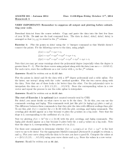
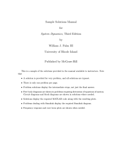
© Copyright 2026