
Sample Solutions Manual for System Dynamics, Third Edition by
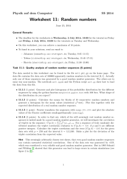
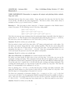
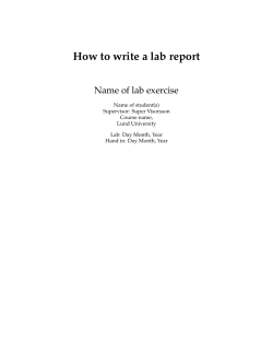
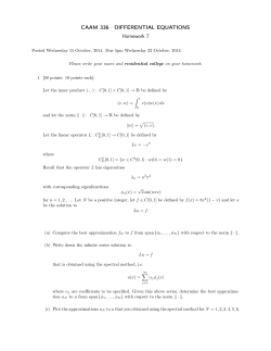
Sample Solutions Manual
for
System Dynamics, Third Edition
by
William J. Palm III
University of Rhode Island
Published by McGraw-Hill
This is a sample of the solutions provided in the manual available to instructors. Note
that
• A solution is provided for very problem, and all solutions are typeset.
• There is only one problem per page.
• Problem solutions display the intermediate steps, not just the final answer.
• Free body diagrams are shown in problems requiring derivation of equations of motion.
Circuit diagrams and block diagrams are shown in solutions where needed.
• Solutions display the required MATLAB code along with the resulting plots.
• Problems dealing with Simulink display the required Simulink diagram.
• Frequency response and root locus plots are shown when needed.
In the solutions manual there is only one problem per page. Problem solutions display the
intermediate steps, not just the final answer.
Problem 2.22 The denominator roots are s = −3 and s = −5, which are distinct. Factor
the denominator so that the highest coefficients of s in each factor are unity:
X(s) =
7s + 4
1
7s + 4
=
2
2s + 16s + 30
2 (s + 3)(s + 5)
The partial-fraction expansion has the form
1
7s + 4
C1
C2
X(s) =
=
+
2 (s + 3)(s + 5)
s+3 s+5
Using the coefficient formula (2.4.4), we obtain
7s + 4
7s + 4
17
C1 = lim (s + 3)
= lim
=−
s→−3
s→−3 2(s + 5)
2(s + 3)(s + 5)
4
C2 = lim
s→−5
(s + 5)
7s + 4
7s + 4
31
= lim
=
s→−5 2(s + 3)
2(s + 3)(s + 5)
4
Using the LCD method we have
1
7s + 4
C1
C2
C1 (s + 5) + C2 (s + 3)
=
+
=
2 (s + 3)(s + 5)
s+3 s+5
(s + 3)(s + 5)
=
(C1 + C2 )s + 5C1 + 3C2
(s + 3)(s + 5)
Comparing numerators, we see that C1 + C2 = 7/2 and 5C1 + 3C2 = 4/2 = 2, which give
C1 = −17/4 and C2 = 31/4.
The inverse transform is
x(t) = C1 e−3t + C2 e−5t = −
17 −3t 31 −5t
e
+ e
4
4
In this example the LCD method requires more algebra, including the solution of two
equations for the two unknowns C1 and C2 .
c 2014 McGraw-Hill. This work is only for non-profit use by instructors in courses for which
the textbook has been adopted. Any other use without publisher’s consent is unlawful.
Free body diagrams are shown in problems requiring derivation of equations of motion.
Circuit diagrams and block diagrams are shown in solutions where needed.
Problem 3.41 See the following figure. Summing forces in the x and y directions gives:
maGx = µs NB − mg sin θ
NA + NB = mg cos θ
(1)
(2)
Summing moments about G:
NA LA − NB LB + µs NB H = 0
(3)
Solve (2) and (3):
NA =
mg cos θ (µs H − LB )
16, 677 cos θ (µs − 2.1)
=
µs H − LA − LB
µs − 4.6
NB = −
mgLA cos θ
40, 025µs cos θ
=
µs H − LA − LB
4.6 − µs
The maximum acceleration is, from (1),
aGx =
23.544µs cos θ
− 9.81 sin θ
4.6 − µs
Figure : for Problem 3.41
c 2014 McGraw-Hill. This work is only for non-profit use by instructors in courses for which
the textbook has been adopted. Any other use without publisher’s consent is unlawful.
Problems dealing with Simulink display the required Simulink diagram.
Problem 5.53 The model is shown in the following figure. Set the Start and End of the
Dead Zone to −0.5 and 0.5 respectively. Set the Sine Wave block to use simulation time.
Set the Amplitude to 2 and the Frequency to 4. In the Math Function block select the
square function. Set the Initial condition of the Integrator to 1. You can plot the results
by typing
plot(tout,simout),xlabel(0t0 ),ylabel(0x0 )
Using a stop time of 3 results in an error message that indicates that Simulink is having
trouble finding a small enough step size to handle the rapidly decreasing solution. By
experimenting with the stop time, we find that, to two decimal places, a stop time of 1.49
will not generate an error.
This model is unstable, and the output x → −∞ if the time span is long enough. We
can see this by writing the equation as (not including the effect of the dead zone)
x˙ = 2 sin 4t − 10x2
Once x drops below
negative values.
p
2/10, x˙ remains negative and thus x continues to decrease through
Figure : for Problem 5.53.
c 2014 McGraw-Hill. This work is only for non-profit use by instructors in courses for which
the textbook has been adopted. Any other use without publisher’s consent is unlawful.
Solutions display the required MATLAB code along with the resulting plots.
Problem 6.49 The script file is
KT = 0.2; Kb = 0.2; c = 5e-4; Ra = 0.8; La = 4e-3; I = 5e-4;
den = [La*I, Ra*I + c*La, c*Ra + Kb*KT];
% Speed transfer function:
sys1 = tf(KT, den);
% Current transfer function:
sys2 = tf([I, c], den);
% Applied voltage
t = [0:0.001:0.05]; va = 10*ones(size(t));
% Speed:
om = lsim(sys1, va, t);
% Current:
ia = lsim(sys2, va, t);
subplot(2,1,1), plot(t, om),xlabel(0 t (s)0 ),ylabel(0\omega (rad/s)0 )
subplot(2,1,2), plot(t, ia),xlabel(0 t (s)0 ),ylabel(0i_a (A)0 )
The plot is shown in the following figure. The peak current is approximately 8 A. The
more accurate value of 8.06 A can be found with the lsim(sys2, va, t) function by
right-clicking on the plot, selecting Characteristics, then Peak Response.
60
ω (rad/s)
50
40
30
20
10
0
0
0.005
0.01
0.015
0.02
0.025
t (s)
0.03
0.035
0.04
0.045
0.05
0
0.005
0.01
0.015
0.02
0.025
t (s)
0.03
0.035
0.04
0.045
0.05
10
8
ia (A)
6
4
2
0
−2
Figure : for Problem 6.49
c 2014 McGraw-Hill. This work is only for non-profit use by instructors in courses for which
the textbook has been adopted. Any other use without publisher’s consent is unlawful.
Frequency response plots are shown when needed.
Problem 9.43 The program is given below, along with the resulting plot. The resonant
frequency is 2.51 × 10⁴ rad/s. By moving the cursor along the plot we can determine the
points at which the curve is 3 dB below the peak. These frequencies are 2.39 × 10⁴ and
2.61 × 10⁴ , so the bandwidth is (2.61 − 2.39) × 104 = 2.2 × 10³ rad/sec.
m = 0.002;k = 1e6;Kf = 20;Kb = 15;R = 10;L = 0.001;
sys = tf(Kf,[m*L,m*R,k*L+Kf*Kb,k*R]);
bode(sys)
Bode Diagram
−100
Magnitude (dB)
−120
−140
−160
−180
−200
Phase (deg)
−220
0
−90
−180
−270
2
10
3
10
4
10
5
10
6
10
Frequency (rad/sec)
Figure : Plot for Problem 9.43
c 2014 McGraw-Hill. This work is only for non-profit use by instructors in courses for which
the textbook has been adopted. Any other use without publisher’s consent is unlawful.
Root locus plots are shown when needed.
Problem 11.57 The characteristic equation is 10s3 + (2 + KD )s2 + KP s + KI = 0. With
KP = 55 and KD = 58, we have 10s3 + 60s2 + 55s + KI = 0, or
1+
KI
1
=0
3
10 s + 6s2 + 5.5s
The root locus gain is K = KI /10. In MATLAB type
sys = tf(1, [1, 6, 5.5, 0]);
rlocus(sys), axis equal
The plot follows. In Example 10.7.4, KI = 25. This gives ζ = 0.707 and τ = 2. The plot
shows that to reduce the error by increasing KI , the dominant time constant will become
larger and the damping ratio will decrease, making the system slower and more oscillatory.
Moving the cursor along the plot shows that if we decrease the error by half by doubling
KI to 50, the new damping ratio will be approximately 0.44 and the new time constant will
be approximately 1/0.43 = 2.3.
Root Locus
15
10
Imaginary Axis
5
0
−5
−10
−15
−20
−15
−10
−5
Real Axis
0
5
10
Figure : for Problem 11.57.
c 2014 McGraw-Hill. This work is only for non-profit use by instructors in courses for which
the textbook has been adopted. Any other use without publisher’s consent is unlawful.


© Copyright 2026