
Full version (19/4/2015)
Pseudorandom generators with optimal seed length for non-boolean
poly-size circuits
Ronen Shaltiel∗
University of Haifa
Sergei Artemenko
University of Haifa
April 19, 2015
Abstract
A sampling procedure for a distribution P over {0, 1}ℓ , is a function C : {0, 1}n → {0, 1}ℓ
such that the distribution C(Un ) (obtained by applying C on the uniform distribution Un ) is
the “desired distribution” P . Let n > r ≥ ℓ = nΩ(1) . An ϵ-nb-PRG (defined by Dubrov and
Ishai (STOC 2006)) is a function G : {0, 1}r → {0, 1}n such that for every C : {0, 1}n → {0, 1}ℓ
in some class of “interesting sampling procedures”, C ′ (Ur ) = C(G(Ur )) is ϵ-close to C(Un ) in
statistical distance.
We construct poly-time computable nb-PRGs with r = O(ℓ) for poly-size circuits relying
on the assumption that there exists β > 0, and a problem L in E = DTIME(2O(n) ) such that
for every large enough n, nondeterministic circuits of size 2βn that have NP-gates cannot solve
L on inputs of length n. This assumption is a scaled nonuniform analogue of (the widely believed) EXP ̸= ΣP
2 , and similar assumptions appear in various contexts in derandomization.
Previous nb-PRGs of Dubrov and Ishai have r = Ω(ℓ2 ) and are based on very strong cryptographic assumptions, or alternatively, on non-standard assumptions regarding incompressibility
of functions on random inputs. When restricting to poly-size circuits C : {0, 1}n → {0, 1}ℓ with
Shannon entropy H(C(Un )) ≤ k, for ℓ > k = nΩ(1) , our nb-PRGs have r = O(k). The nb-PRGs
of Dubrov and Ishai use seed length r = Ω(k 2 ) and require that the probability distribution of
C(Un ) is efficiently computable.
Our nb-PRGs follow from a notion of “conditional PRGs” which may be of independent
interest. These are PRGs where G(Ur ) remains pseudorandom even when conditioned on a
“large” event {A(G(Ur )) = 1}, for an arbitrary poly-size circuit A. A related notion was considered by Shaltiel and Umans (CCC 2005) in a different setup, and our proofs use ideas from
that paper, as well as ideas of Dubrov and Ishai.
We also give an unconditional construction of a poly-time computable nb-PRGs for poly(n)size, depth d circuits C : {0, 1}n → {0, 1}ℓ with r = O(ℓ · logd+O(1) n). This improves upon the
previous work of Dubrov and Ishai that has r ≥ ℓ2 . This result follows by adapting a recent
PRG construction of Trevisan and Xue (CCC 2013) to the case of nb-PRGs, and implementing
it by constant-depth circuits.
∗
This research was supported by BSF grant 2010120, ISF grant 864/11, and ERC starting grant 279559.
1
1
Introduction
A sampling procedure is a function C : {0, 1}n → {0, 1}ℓ such that when C is applied on the uniform
distribution Un , the obtained distribution C(Un ) is some “desired distribution” P over ℓ-bit strings.
There are two natural complexity measures for sampling procedures: the computational complexity
of the function C, and the randomness complexity which is the number of random bits used by the
procedure (denoted here by n). The reader is referred to [Vio12], for a discussion on the complexity
of sampling procedures.
Dubrov and Ishai [DI06] considered the following natural problem: is it possible to reduce the
randomness complexity of sampling procedures without substantially increasing their computational complexity? Specifically, given an efficient sampling procedure C : {0, 1}n → {0, 1}ℓ with
n > ℓ, construct an efficient sampling procedure C ′ : {0, 1}r → {0, 1}ℓ which uses only r ≪ n
random bits, and C ′ (Ur ) is close to the desired distribution C(Un ) in statistical distance.1 For
this purpose, Dubrov and Ishai suggested the following notion of “pseudorandom generator against
non-Boolean statistical tests”.
Definition 1.1 (nb-PRG [DI06]). A function G : {0, 1}r → {0, 1}n is an ϵ-nb-PRG for a function
C : {0, 1}n → {0, 1}ℓ if the distributions C(G(Ur )) and C(Un ) are ϵ-close (and we say that G ϵ-fools
C). G is an ϵ-nb-PRG for a class C of functions, if G is an ϵ-nb-PRG for every function in the
class.
Indeed, given an efficient nb-PRG G we can compute C ′ (Ur ) = C(G(Ur )) and sample a distribution that is ϵ-close to C(Un ) using only r random bits.2 Note that if the class of sampling
procedures that we consider contains the function C : {0, 1}n → {0, 1}ℓ that outputs the first ℓ bits
(and any reasonable complexity class does), then the seed length r has to be at least ℓ (assuming
ϵ < 1/2).
The notion of nb-PRGs is a natural generalization of “standard PRGs” defined below.
Definition 1.2 (PRG). A function G : {0, 1}r → {0, 1}n is an ϵ-PRG for a function C : {0, 1}n →
{0, 1} if | Pr[C(G(Ur )) = 1] − Pr[C(Un ) = 1]| ≤ ϵ (that is iff C(G(Ur )) and C(Un ) are ϵ-close). G
is an ϵ-PRG for a class C of functions, if G is an ϵ-PRG for every function in the class.
Consequently, nb-PRGs are at least as hard to construct as (standard) PRGs. In this paper
we will be interested nb-PRGs for two types of sampling procedures: polynomial-size circuits (for
which we will have to rely on unproven assumptions) and circuits with polynomial-size and constant
depth (for which we can expect and obtain unconditional constructions).
If H(C(Un )) is small. If we are guaranteed that the Shannon entropy of C(Un ) is small (say
H(C(Un )) ≤ k for some parameter k < ℓ) than we can hope for a shorter seed length r ≈ k (which
can be smaller than ℓ). As we now explain, in this setup the best seed length that we can expect
is k/ϵ. This is because there are efficiently samplable distributions P with entropy k, such that
any distribution that is ϵ-close to P cannot be sampled using less than Ω(k/ϵ) bits.3 Thus, an
1
Two distributions over the same domain are ϵ-close if the probability that they assign to any event differs by at
most ϵ.
2
It is important to observe that C ′ (Ur ) is required to be statistically indistinguishable from C(Un ). Standard
PRGs suffice if we relax the requirement to computational indistinguishability.
3
Let 2−n ≤ ϵ ≤ 1/10. Fix some x ∈ {0, 1}n and consider the distribution P over {0, 1}n which gives weight 1 − 4 · ϵ
to x and 4 · ϵ/(2n − 1) to every other string. Note that H(P ) = O(ϵn), and yet, for every distribution Q that is
samplable using less than n/2 random bits, Q is not ϵ-close to P .
1
ϵ-nb-PRG for poly-size circuits that are guaranteed to produce distributions with entropy ≤ k,
must have seed length r = Ω(k/ϵ).
1.1
nb-PRGs for polynomial-size circuits
The setup. The most natural setup of parameters for sampling procedures is the case of sampling
procedures C where the input length n, output length ℓ and the size of C are all polynomially
related, and we fix this choice of parameters for this discussion. For the application of reducing
randomness for sampling procedures, the size of C is known to the PRG, and the PRG may
be allowed to run in time p(n) for a polynomial p that is larger than the size of C. In the
terminology of PRGs, this setup is often referred to as the “Nisan-Wigderson setting” [NW94].
However, note that as ℓ = nΩ(1) and the seed length must be at least ℓ, we are interested in PRGs
O(1)
G : {0, 1}r → {0, 1}r
(often referred to as polynomial stretch). The application also dictates
that G runs in time polynomial in r. This is in contrast to the standard “Nisan-Wigderson setting”
in which PRGs are often allowed to run in time exponential in their seed length (because intended
applications plan to enumerate all seed anyway).4
Using cryptographic PRGs. A very natural approach to construct nb-PRGs is to reduce to
constructing standard PRGs. It is immediate that a standard PRG for circuits of size s + 2ℓ
is an nb-PRG for circuits C : {0, 1}n → {0, 1}ℓ of size s. (This is because any statistical test
on ℓ bits can be implemented by a circuit of size 2ℓ ). This means that a (standard) PRG G :
Ω(1)
{0, 1}r → {0, 1}n that fools circuits of size s+2ℓ = 2n
is an nb-PRG with the desired parameters.
These parameters are obviously impossible in the Nisan-Wigderson setting (where a PRG that
runs in polynomial time cannot fool a circuit of size superpolynomial). However, one can hope to
achieve such parameters using “cryptographic PRGs” such as the Blum-Micali-Yao [BM84, Yao82]
or HILL [HILL99, HHR11, Hol06, HRV10]. Such PRGs imply (and therefore require) cryptographic
assumptions such as the existence of one-way functions. Indeed, Dubrov and Ishai observe that
if there exist one-way permutations f : {0, 1}r → {0, 1}r that cannot be inverted with noticeable
probability by circuits of size 2O(ℓ) , then the PRG construction of Blum, Miali and Yao [BM84,
Yao82] gives an nb-PRG with seed length r. A weakness of this approach is that in order to
achieve seed length r = O(ℓc ) we need one-way permutations that cannot be inverted by circuits
1/c
of size 2Ω(r ) . This means that we can achieve seed length r = O(ℓ) only if we have permutations
that cannot be inverted with noticeable probability by size 2Ω(r) circuits. This is a very strong
assumption that is known not to hold for some of the candidate one-way permutations. This
assumption becomes plausible for constants c ≫ 1 and gives nb-PRGs with seed length r = O(ℓc ).5
Dubrov and Ishai also show that this approach also yields nb-PRGs with seed length r =
O((k/ϵ)c ) for polynomial-size circuits C which are guaranteed to sample distributions with Shannon
entropy ≤ k.6
4
We remark that a similar setup (in the boolean setting) arises in “typically-correct derandomization” [Sha11,
KvMS12, Sha10].
5
One can also consider starting from one-way functions (rather than permutations) but the best known PRG
constructions from one-way functions [HILL99, HHR11, Hol06, HRV10] have a polynomial blow-up in the seed length.
6
This is achieved by showing that there exists a circuit D : {0, 1}ℓ → {0, 1}O(k/ϵ) of size roughly 2k such that if
C(Un ) and C(G(Ur )) are not ϵ-close then D(C(Un )) and D(C(G(Ur )) are not Ω(ϵ)-close, meaning that an nb-PRG
that fools D ◦ C also fools C, and in this setup an nb-PRG can handle very large circuits anyway. Note that this
reduction is specific to this setup in which the PRG can fool very large circuits.
2
Function compression. Dubrov and Ishai show an interesting connection between nb-PRGs and
“function compression”. A function f : {0, 1}n → {0, 1} is compressed by a circuit C : {0, 1}n →
{0, 1}ℓ if an unbounded procedure can compute f (x) given C(x) (without receiving x). We say that
f is (1/2 + ϵ, ℓ)-compressible by size s circuits, if there exists a size s circuit C : {0, 1}n → {0, 1}ℓ
and a function D such that f (x) = D(C(x)) on at least (1/2 + ϵ)-fraction of the inputs. Dubrov
and Ishai suggested to base nb-PRG constructions on the assumption that there exist explicit
incompressible boolean functions.7
Nisan-Wigderson PRG with incompressible functions. Dubrov and Ishai show that a polynomial time computable nb-PRG that fools circuits of size nc is obtained under the following assumption: There is a function f : {0, 1}O(ℓ) → {0, 1} computable in polynomial time that is not
(1/2 + Ω(ϵ/ℓ), Ω(l))-compressible by circuits C : {0, 1}n → {0, 1}ℓ of size nO(c) . This result follows
by using the function f in the Nisan-Wigderson generator [NW94], and follows by a clever argument showing that the security proof of [NW94] applies in this setting. However, a well known
inefficiency of the Nisan-Wigderson generator dictates that even under this assumption the obtained seed length cannot be linear in ℓ and must be at least quadratic, that is r = Ω(ℓ2 ). This
inefficiency was the focus of several works that construct improved PRGs (in the boolean setting)
[ISW06, SU05, Uma03, Uma09], but all these approaches give PRGs with running time exponential
in the seed length. Consequently, these approaches do not make sense in our setup where PRGS
are required to run in time polynomial in the seed length.
1.1.1
Hardness assumptions for exponential size circuits
We give new constructions of nb-PRGs in the “Nisan-Wigderson setting”. Our constructions achieve
seed length r = O(ℓ) under strong but plausible assumptions. In order to discuss our assumptions
we need a quick review of nondeterministic circuits and oracle circuits.
Definition 1.3 (nondeterministic circuits and oracle circuits). A non-deterministic circuit C has
additional “nondeterministic input wires”. We say that the circuit C evaluates to 1 on x iff there
exist an assignment to the nondeterministic input wires that makes C output 1 on x. Given a
boolean function A(x), an A-circuit is a circuit that is allowed to use A gates (in addition to the
standard gates). An NP-circuit is a SAT-circuit (where SAT is the satisfiability function) a Σi circuit is an A-circuit where A is the canonical ΣPi -complete language. The size of all circuits is
the total number of wires and gates.8
7
The high level idea is that some PRG constructions in the literature, are proven by a reduction showing that a
small distinguisher circuit for the PRG can be converted into a small circuit computing the supposedly hard function.
Some of these reductions can also convert a non-boolean distinguisher into a non-boolean circuit that compresses the
function. This approach allows using one-way permutations f : {0, 1}r → {0, 1}r against poly-size circuits (rather
than exponential size circuits), if the permutations have hard-core bits that are not only secure, but are also not
(1/2 + r−ω(1) , Ω(r))-compressible by polynomial size circuits. Assuming the existence of such one-way permutations,
Dubrov and Ishai show that the Blum-Micali-Yao PRG yields an nb-PRG and has seed length r = O(ℓ). We are not
aware of research that attempts to evaluate the validity of this assumption. We also point out, that this nb-PRG does
not extend to have seed length proportional to the entropy, when it is guaranteed that the entropy of the sampled
distribution C(Un ) is small.
8
An alternative approach is to define using the Karp-Lipton notation for Turing machines with advice. For
s ≥ n, a size sΘ(1) deterministic circuit is equivalent to DTIME(sΘ(1) )/sΘ(1) , a size sΘ(1) nondeterministic circuit
is equivalent to NTIME(sΘ(1) )/sΘ(1) , a size sΘ(1) NP-circuit is equivalent to DTIMENP (sΘ(1) )/sΘ(1) , a size sΘ(1)
nondeterministic NP-circuit is equivalent to NTIMENP (sΘ(1) )/sΘ(1) , and a size sΘ(1) Σi -circuit is equivalent to
3
Note for example that an NP-circuit is different than a nondeterministic circuit. The former is a
nonuniform analogue of PNP (which contains coNP) while the latter is an analogue of NP. Similarly,
NP and is thus weaker than
a nondeterministic NP-circuit is the nonuniform analogue of ΣP
2 = NP
P
a Σ2 -circuit (which is analogous to PΣ2 ). Hardness assumptions against nondeterministic/NP/Σi
circuits appear in the literature in various contexts of derandomization [KvM02, MV05, TV00,
GW02, SU05, SU06, BOV07]. Typically, the assumption is of the following form: E is hard for
exponential size circuits (where the type of circuits is one of the types discussed above). More
specifically:
Definition 1.4. We say that “E is hard for exponential size circuits of type X” if there exists a
problem L in E = DTIME(2O(n) ) and a constant β > 0, such that for every sufficiently large n,
circuits of type X with size 2βn fail to compute the characteristic function of L on inputs of length n.
Such assumptions can be seen as the nonuniform and scaled-up versions of assumptions of the
form EXP ̸= NP or EXP ̸= ΣP
2 (which are widely believed in complexity theory). As such, these
assumptions are very strong, and yet plausible - the failure of one of these assumptions will force
us to change our current view of the interplay between time, nonuniformity and nondeterminism.9
1.1.2
New constructions of nb-PRGs for poly-size circuits
We give a construction of nb-PRGs with seed length r = O(ℓ) under the assumption that E is hard
for exponential size nondeterministic NP-circuits.
Theorem 1.5 (nb-PRGs with short seed). There is a constant b > 1 such that if E is hard for
exponential size nondeterministic NP-circuits then for every constants e > 0 and c > 1 there is a
poly(n)-time computable ϵ-nb-PRG G : {0, 1}b·ℓ → {0, 1}n for size nc circuits C : {0, 1}n → {0, 1}ℓ ,
as long as ℓ ≥ ne , ϵ ≥ n−c .
Note that G runs in time polynomial in n and this polynomial is allowed to depend on c, e. We
remark that the assumption that ℓ ≥ ne in Theorem 1.5 can be omitted and then we require that
ϵ ≥ ℓ−c . The reader is referred to Remark 1.8 for an explanation.
If the entropy of C(Un )) is small. We also consider the subclass of poly-size circuits C such
that H(C(Un )) ≤ k. Recall that here, the best we can shoot for is seed length r = O(k/ϵ). We
achieve this under the same hardness assumption.
Theorem 1.6 (nb-PRGs for low entropy procedures). There is a constant b > 1 such that if
E is hard for exponential size nondeterministic NP-circuits then for every constants e > 0 and
c > 1 there is a poly(n)-time computable ϵ-nb-PRG G : {0, 1}b·k/ϵ → {0, 1}n for size nc circuits
C : {0, 1}n → {0, 1}ℓ which satisfy H(C(Un )) ≤ k, as long as k ≥ ne , ℓ ≤ nc .
P
DTIMEΣi (sΘ(1) )/sΘ(1) . With this view, we can also differentiate between circuits that make adaptive calls to their
oracle, and circuits that make nonadaptive calls to their oracle, and the latter are called parallel circuits.
9
Another advantage of constructions based on this type of assumptions is that any E-complete problem (and such
problems are known) can be used to implement the constructions, and the correctness of the constructions (with that
specific choice) follows from the assumption. We do not have to consider and evaluate various different candidate
functions for the hardness assumption.
4
Again, the polynomial running time of G is allowed to depend on c, e, and that the requirement
thaet k ≥ ne can be removed, adding the requirement that ϵ ≥ k −c . Following the discussion
in previous sections, we point out that in this setup, nb-PRGs with this seed length were only
known under the assumption that there are one-way permutations with hardness 2Ω(n) , and this is
known not to hold for some candidate one-way permutations. Dubrov and Ishai [DI06] were able
to achieve nb-PRGs in this setup under some of the other assumptions discussed in Section 1.1.
However, these nb-PRGs achieve seed length ≥ (k/ϵ)2 , and require an additional assumption: that
it is feasible to compute the quantity p(z) = Pr[C(Un ) = z] given z ∈ {0, 1}ℓ .
Alternative hardness assumptions for our theorems. We have chosen to state a hardness
assumption in Theorems 1.5 and 1.6. However, in the technical construction will rely on the
assumption that there are (boolean) PRGs in a certain setup. The precise assumption is stated
below.
Assumption 1.7. For every constant c > 1 there exists an (n−c )-PRG G′ : {0, 1}n → {0, 1}n for
nondeterministic NP-circuits of size nc , and G′ is computable in time p(n) where p is a polynomial
that depends on c.
c
This assumption is known to follow from the assumption stated in Theorems 1.5 and 1.6 by
the following argument: By the “downward collapse theorem” of Shaltiel and Umans [SU06] the
assumption that E is hard for exponential size nondeterministic NP circuits implies that E is hard
for exponential size Σ2 -circuits that make non-adaptive calls to their oracle. By [KvM02, IW97]
the latter assumption implies a PRG G′ with the required properties.
In fact, the PRG G′ obtained in [IW97, KvM02] has better parameters than we asked for. It
has “exponential stretch” and stretches O(c · logn) bits into nc bits.
Remark 1.8. Using this stronger version of assumption 1.7 allows us to prove versions of Theorem
1.5 (respectively Theorem 1.6) in which the assumption that ℓ ≥ ne (respectively k ≥ ne ) and then
the seed length is O(ℓ + log n) (respectively O(k/ϵ + log n)). This implication follows by the same
proofs, and is explained in Remark 3.3.
Indeed, the assumption stated in Theorems 1.5 and 1.6 is stronger than what is actually needed
(as we only need the PRG of assumption 1.7 to have polynomial stretch). We can therefore use a
hardness assumption against polynomial size Σ2 -circuits (rather than circuits of almost exponential
size). However, as we are shooting for a PRG which is computable in polynomial time (rather than
exponential time), we cannot afford “worst-case to average-case hardness amplification” (which
takes exponential time and is known not to be possible in polynomial time by black-box techniques
[Vio05]). Instead, we can use Yao’s XOR-Lemma (see [GNW95] for a survey) which does not
blow up the running time. The price of this modification is that instead of a “worst-case hardness
assumption” we require a “mildly average-case hardness assumption”. Summing up, we get that
Assumption 1.7 (and therefore the conclusion of the two main theorems) also follow from the
following assumption:
Assumption 1.9. For every constant c > 1 there exists a problem L in P such that for every
sufficiently large n, every size nc Σ2 -circuit fails to compute the characteristic function of L on at
least a 1/n-fraction of the inputs of length n.
5
This assumption gives assumption 1.7 by using Yao’s XOR-Lemma on (the characteristic function of) L, and then plugging the amplified function to the Nisan-Wigderson generator. We remark
that the same assumption is also suggested (and relied on) in a construction of Goldreich and
Wigderson [GW02] in a different context.
1.2
New constructions of nb-PRGs for constant-depth circuits
In this section we discuss unconditional constructions of nb-PRGs against poly-size circuits that
have constant-depth. There are many surprising instances where interesting distributions can be
sampled by procedures with very low computational complexity see e.g., [AIK06] and following
work. The reader is referred to [Vio12] for examples of low complexity sampling procedures.
Dubrov and Ishai [DI06] considered the following setup: Let c, d, e be positive constants and
consider a sampling procedure C : {0, 1}n → {0, 1}ℓ that is a circuit of size nc and depth d
which outputs ℓ = ne bits. Note that this is the setup considered in the previous section, with
the additional restriction that circuits have constant depth. Dubrov and Ishai gave the following
construction of nb-PRG.
Theorem 1.10. [DI06] Let c, d, e be positive constants. For every constant δ > 0 there is an ϵ-nbPRG G : {0, 1}r → {0, 1}n for circuits of size nc , depth d and output length ℓ = ne . Furthermore,
r = ℓ2+δ , ϵ = n−ω(1) and G is computable in time poly(n).
The construction of Dubrov and Ishai uses the Nisan-Wigderson generator [Nis91, NW94] with
the parity function, and is based on showing that the parity function cannot be compressed by
small constant-depth circuits. However, the aforementioned bottleneck in the Nisan-Wigderson
generator causes the seed length r to be larger than ℓ2 whereas the obvious lower bound is (once
˜
again) ℓ. Our first result is an nb-PRG which achieves seed length O(ℓ).
Theorem 1.11 (nb-PRGs with short seed). Let c, d, e be positive constants. There is an ϵ-nb-PRG
G : {0, 1}r → {0, 1}n for circuits of size nc , depth d and output length ℓ = ne . Furthermore,
r = O(ℓ · logad n) (where ad = d + O(1) is a constant that depends only on d), ϵ = n−ω(1) and G is
computable in time poly(n).
Our construction gives a general result for arbitrary size, depth, output length and error, and
Theorem 1.11 above is a special case of a more general theorem that is stated and proven in Section
5. Our proof is based on adapting a recent boolean PRG construction of Trevisan and Xue [TX12]
(which avoids the Nisan-Wigderson generator) to the case on nb-PRGs.
A drawback of both Theorem 1.10 and Theorem 1.11 is that the pseudorandom generator
G is guaranteed to run in polynomial time, but is not necessarily implementable by a poly-size
circuit with constant depth. This means that if we use G to sample the output distribution of
some sampling procedure C : {0, 1}n → {0, 1}ℓ that is a poly-size constant depth circuit, then the
resulting sampling procedure C ′ (·) = C(G(·)) is implementable in poly-time but not necessarily in
constant depth. Our next result gives an nb-PRG which is implementable by a uniform family of
poly-size constant depth circuits. This PRG achieves seed length roughly ℓ1+α (where α > 0 is an
arbitrary small constant). This is worse than the seed length of Theorem 1.11, but still better than
that achieved by Dubrov and Ishai in Theorem 1.10.
Theorem 1.12 (nb-PRGs implementable in constant depth). Let c, d, e be integer constants. For
every α > 0 there is an ϵ-nb-PRG G : {0, 1}r → {0, 1}n for circuits of size nc , depth d and output
6
length ℓ = ne . Furthermore, r = O(ℓ1+α · logad n) (where ad = O(1/α + d) is a constant that
depends only on d, α), ϵ = n−ω(1) and G is computable by a family of uniform circuits of size
poly(n, c log n) and depth O(1/α) (where the constant hidden in the O(·) is universal, and the depth
does not depend on c, d).10
Once again, a more general theorem with more parameters is stated and proven in Section 5.
We obtain this result, by giving an implementation of a variant of the nb-PRG of Theorem 1.11
by constant depth circuits. For this, we use an approach of Viola [Vio12] to show that k-wise
independent distributions can be sampled with competitive seed length by constant depth circuits.
We stress that the nb-PRG of Dubrov and Ishai from Theorem 1.10 is not computable by small
constant depth circuits. This is because it computes the parity function on inputs of length ≥ ℓ.
2
Technique
We aim to reduce the task of constructing nb-PRGs to that of constructing standard PRGs. Our
first attempt is the following trivial observation: An (ϵ/2ℓ )-PRG for size s + O(ℓ) circuits is also
an ϵ-nb-PRG for size s circuits. This follows because if C(Un ) and C(G(Ur )) are not ϵ-close, then
there exists z ∈ {0, 1}ℓ such that the probability assigned to z by the two distributions differ by
ϵ/2ℓ . This means that a boolean circuit C ′ (x) which outputs 1 iff C(x) = z is not (ϵ/2ℓ )-fooled
by G.
Using the Nisan-Wigderson generator, we can construct such PRGs given a poly-time computable function f : {0, 1}O(ℓ) → {0, 1} on which every circuit of size sO(1) errs on at least
a (1/2 − 1/2O(ℓ) )-fraction of inputs. (Because of the aforementioned inefficiency of the NisanWigderson PRG, this approach cannot give seed smaller than Ω(ℓ2 )). However, “existing techniques” cannot produce such a function f from the assumption that E is hard for exponential
size circuits (or even from the weaker assumption: E is mildly average-case hard for exponential
size circuits) [SV10, AS14]. Trevisan and Vadhan [TV00] suggested that these limitations can be
bypassed if we assume that E is hard for exponential size nondeterministic circuits (or more generally Σi -circuits for some i ≥ 1). They were able to start from such assumptions and obtain their
goal (which is extractors for samplable distributions). They were not, however, able to construct
average-case hard functions (or PRGs) with very low error.
Inspired by the success of Trevisan and Vadhan, we aim to construct nb-PRGs starting from a
worst-case hardness assumption for Σi -circuits (for some small i). In order to achieve this, we would
like a reduction, showing that a circuit C : {0, 1}n → {0, 1}ℓ that is not ϵ-fooled by some candidate
PRG can be transformed into a boolean test that is not ϵ′ -fooled by the PRG. Our boolean test
may be complex (and allowed to use nondeterminism) but we require that ϵ′ is not much smaller
than ϵ. This intuition is captured in the following lemma (which can be seen as a more careful
version of our first attempt).
Lemma 2.1. There exists a constant B1 > 0 such that for every constant B2 > 0 the following
holds: Let R and V be distributions over {0, 1}ℓ that are not ℓ−B2 -close (the reader should think of
R = C(Un ) and V = C(G(Ur ))). There exist a z ∈ {0, 1}ℓ and i ∈ [ℓ] such that
| Pr[Ri = zi |R1,...,i−1 = z1,...,i−1 ] − Pr[Vi = zi |V1,...,i−1 = z1,...,i−1 ]| > ℓ−(B2 +5) ,
10
Note that this nb-PRG is “cryptographic” in the sense that the PRG is implementable by a uniform family of
′
circuits of size nc and depth d′ , for some constants c′ , d′ and is able to fool circuits of depth d and size nc for larger
d, c for every sufficiently large n.
7
and Pr[R1,...,i−1 = z1,...,i−1 ] ≥ 2−B1 ·ℓ .
Lemma 2.1 follows by iteratively using the following easy lemma.
Lemma 2.2. Let SD(P, Q) denote the statistical distance between P and Q. Let R, V be two
distributions over some finite set S, such that SD(R; V ) ≥ α. Let ρ, ν ≥ 0 and let f : S → {0, 1}
be a function such that p = Pr[f (R) = 0] ≤ 21 then at least one of the following holds:
• | Pr[f (R) = 1] − Pr[f (V ) = 1]| > ρ.
• SD((R|f (R) = 1); (V |f (V ) = 1)) ≥ (α − ρ) · (1 − ν).
• SD((R|f (R) = 0); (V |f (V ) = 0)) ≥ (α − ρ) · (1 + ν/2p).
Indeed, with the choices above, the lemma says that if R and V are statistically far, then either
the boolean function f (x) = x1 distinguishes them, or else, we can condition on the value of the
first bit and still have large statistical distance. Conditioning decreases ℓ by one, and so we make
progress. Eventually we will find an index i that distinguishes R and V (conditioning on previous
values).
Some care must be used in this argument, as we want the probability of the final event that
we condition on to be 2−Ω(ℓ) . This is the reason that the statement of Lemma 2.2 states (in the
third item) that if we condition on an event with probability p that may be very small then the
statistical distance increases in a rate that is inversely proportional to p. The statistical distance
cannot exceed one, and using that, we can argue that the probability of the final event that we
condition on, is not too small. The precise argument (and in particular the proofs of Lemma 2.1
and Lemma 2.2) appear in Section 6.
2.1
Conditional tests
The next definition captures the kind of tests that distinguish C(Un ) from C(G(Ur )) according to
the Lemma 2.1.
Definition 2.3 (Conditional test [SU06]). A conditional test is a pair (A, D) where A : {0, 1}n →
{0, 1} is called condition, and D : {0, 1}n → {0, 1} is called distinguisher. We say that a conditional
test (A, D) is ϵ-fooled by a distribution P over {0, 1}n if
| Pr [D(X) = 1|A(X) = 1] − Pr [D(X) = 1|A(X) = 1]| ≤ ϵ
X←P
X←Un
The density of a condition A is PrX←Un [A(X) = 1]. The density of a conditional test (A, D) is
the density of A, and we say that the test has size s if both A, D are circuits of size at most s.
With this terminology, Lemma 2.1 can be rephrased as follows:
Corollary 2.4. There exists a constant B1 > 0 such that for every constant B2 > 0 the following
holds: Let G : {0, 1}r → {0, 1}n , and let C : {0, 1}n → {0, 1}ℓ be a size s circuit. If C is not
ℓ−B2 -fooled by G then there exist a conditional test (A, D) of size s + O(ℓ) and density ≥ 2−B1 ·ℓ
which is not ℓ−(B2 +5) -fooled by G.
8
2.2
PRGs against conditional tests
In light of Corollary 2.4, we would like to construct a PRG that fools poly-size conditional tests.
Shaltiel and Umans [SU06] constructed PRGs against conditional tests. However, the setup considered there is quite different. It is not required that the PRG is computable by a deterministic
procedure, and the PRG is allowed to have access to an NP-oracle. Moreover, the PRG receives
the condition A before producing its output. This allows the PRG to find “interesting” elements
x ∈ {x : A(x) = 1} using its NP oracle, and this ability is critically used by the PRG. There are
also additional advantages to having an NP oracle, which we can’t use in our setup. On the other
hand, we have an advantage over the setup of [SU06]. We are guaranteed that the density of A
is roughly 2−ℓ and are shooting for seed length O(ℓ) (whereas in [SU06] one wants seed O(log n)
regardless of the density).
We are not able to construct polynomial time PRGs against conditional tests in our setup.
However, we are able to achieve the following weaker objects:
Definition 2.5 (cd-PRG). A function G : {0, 1}r1 +r2 → {0, 1}n is an ϵ-cd-PRG for a class C of
conditional tests, if with probability 1 − ϵ/2 over choosing s1 ← Ur1 , every conditional test (A, D)
in C is ϵ/2-fooled by Gs1 (Ur2 ), where Gs1 : {0, 1}r2 → {0, 1}n is defined by Gs1 (s2 ) = G(s1 ◦ s2 ).
G is an ϵ-wcd-PRG if for every conditional test (A, D) in C, with probability 1 − ϵ/2 over choosing
s1 ← Ur1 , (A, D) is ϵ/2-fooled by Gs1 (Ur2 ).
Note that a cd-PRG is in particular a wcd-PRG. Loosely speaking, in both notions, this definition allows the PRG to choose a uniform s1 ∈ {0, 1}r1 which will not be affected by the condition
A. Only the second part of the seed (namely, s2 ) is affected by conditioning.11
We are able to use the machinery developed by Shaltiel and Umans [SU06] (together with
additional ideas) to construct cd-PRGs under the assumption that E is hard for exponential size
nondeterministic NP-circuits, and wcd-PRGs under the weaker assumption that E is hard for
exponential size nondeterministic circuits. We elaborate on this in Section 3.
It is not difficult to show that the stronger notion of cd-PRGs gives nb-PRGs. This follows by
the next lemma.
Lemma 2.6 (cd-PRGs are nb-PRGs). Let B be a constant and let G : {0, 1}r1 +r2 → {0, 1}n be an
(ℓ−(B+5) /2)-cd-PRG for conditional tests of size s + O(ℓ) and density at least 2−O(ℓ) then G is a
ℓ−B -nb-PRG for size s circuits C : {0, 1}n → {0, 1}ℓ .
Proof. Let C : {0, 1}n → {0, 1}ℓ be a circuit of size s and assume that C is not ℓ−B -fooled by G,
meaning that SD(C(G(Ur )), C(Un )) > ℓ−B . By an averaging argument, for an ℓ−B /2-fraction of
s1 ∈ {0, 1}r1 , C is not (ℓ−B /2)-fooled by Gs1 , and call such s1 useful. By Corollary 2.1 for every
useful s1 , there exists a conditional test (As1 , Ds1 ) of size s + O(ℓ) and density 2−O(ℓ) which is not
(ℓ−(B+5) /2)-fooled by Gs1 .
We remark that the fact that Gs1 fools all circuits s + O(ℓ) is an overkill for the argument.
However, we do need Gs1 to fool many tests simultaneously, and this is why the argument does not
work with wcd-PRGs.
For perspective, let us consider an analogous definition to the standard setup of PRGs (or even nb-PRGs): Let C
be a class of functions C : {0, 1}n → {0, 1}ℓ . If for every test in the class C, with probability 1 − ϵ/2, over s1 ← Ur1 ,
Gs1 (Ur2 ) ϵ/2-fools the test, then G is an ϵ-nb-PRG. Thus, for the more standard notion of ϵ-PRGs (or even ϵ-nbPRGs) the modifications made in Definition 2.5 are immaterial and this is why this notion is not usually defined in
these setups.
11
9
2.3
Organization of this paper
In Section 3 we give our main construction of cd-PRGs, prove its correctness, and derive the proof
of Theorem 1.5. In Section 4 we show how to extend the nb-PRG to the case that the entropy of
C(Un ) is small, and prove Theorem 1.6. In Section 5 we give an unconditional constructions of
nb-PRGs for poly-size constant depth circuits, and prove Theorems 1.11 and 1.12. In Section 6 we
prove lemmas 2.2 and 2.1.
3
A construction of cd-PRGs
We now show that Assumption 1.7 implies cd-PRGs. The construction is specified in Figure 1.
The intuition for the construction builds on ideas of Shaltiel and Umans [SU06] (together with
additional ideas) and we give a high level intuition in the next paragraph.
Figure 1: A cd-PRG
Goal: Construct a n−b -cd-PRG for tests of size nb and density ≥ 2−d .
Parameters:
• n - The output length of the cd-PRG
• b, d - The goal is to fool conditional tests of size nb and density ≥ 2−d .
• v = d + O(b · log n) is a parameter set by the construction.
• d1 , d2 - These are seed lengths for PRGs that the construction uses as a black box.
These ingredients are listed below.
Ingredients:
• A family H of 2q permutations, for q = nO(b) , indexed by strings s ∈ {0, 1}q . Given
s, the permutations hs , h−1
are required to be computable in time nO(b) . H should
s
−n11b
10b
be (2
)-close to (n )-wise independent, namely, for every distinct x1 , . . . , xn10b ∈
11b
n
{0, 1} , (hs (x1 ), . . . , hs (xn10b ))s←Uq is 2−n -close to the uniform distribution on n10b
distinct elements from {0, 1}n . There are such explicit constructions in the literature
[Gow96, HMMR05, KNR09].
• A function G1 : {0, 1}d1 → {0, 1}q that is computable in time polynomial in n.
• A function G2 : {0, 1}d2 → {0, 1}n−v that is computable in time polynomial in n.
Both G1 , G2 will be assumed to be pseudorandom generators for nondeterministic NP2
circuits of size nO(b ) which exist by assumption 1.7.
The cd-PRG: G : {0, 1}r:=d1 +d2 +v → {0, 1}n is defined as follows: Given s1 ∈ {0, 1}d1 , s2 ∈
{0, 1}d2 and w ∈ {0, 1}v , we define G(s1 , s2 , w) = h−1
G1 (s1 ) (G2 (s2 ) ◦ w). We set r1 = d1 and
r2 = d2 + v so that r = r1 + r2 .
Intuition for the construction. Recall that we are aiming to construct a cd-PRG for conditional tests with density at least 2−d . The first r1 bits of the seed will be used to select a seed
10
s for a poly(n)-wise independent permutation hs : {0, 1}n → {0, 1}n . This costs r1 > n random
bits (that we cannot afford) and we will derandomize this choice using a PRG G1 for nondeterministic NP-circuits. That is, we use a short seed s1 to sample a permutation hG1 (s1 ) . For the
sake of simplicity of this informal explanation let us pretend that h is a poly(n)-wise independent
permutation. In the actual proof we will argue that the derandomization of h using G1 still allows
the argument below.
Every relevant condition circuit A has density 2−d , meaning that the set {x : A(x) = 1} is of
size at least 2n−d . For simplicity, let us pretend that the size is exactly 2n−d . Let v be a parameter
and let h′ : {0, 1}n → {0, 1}n−v denote the version of h in which we truncate v bits of the output
of h. Intuitively, h′ is a very good hash function and so if we set v to be slightly larger than d (say
v = d + O(b log n)) then w.h.p. h′ will be a good hash function for all relevant circuits. By good,
we mean that for every z ∈ {0, 1}n−v the number of preimages of z that land in {x : A(x) = 1}
is very close to the expected number of 2v−d . (The parameters are chosen so that this indeed
holds for a random nO(b) -wise independent permutation, using a Chernoff bound for independent
permutations (that we prove in Section 3.2) and a union bound over all size nb circuits.) For the
sake of this informal explanation, let us oversimplify, and pretend that this holds even for v = d
and that the hash function h′ is one-to-one over {x : A(x) = 1} for every relevant circuit A. We
will continue our informal explanation under this unjustified (and false) assumption.
At this point, we used our seed s1 to choose a function h, and the definition of cd-PRGs requires
that we need to show that with high probability (over s1 ), we can construct a PRG Gs1 (s2 ) that fools
size nb conditional tests of density 2−d . We use a short seed s2 and apply a PRG G2 against NPcircuits to generate a pseudorandom string G2 (s2 ) of length n − v (recall that we have such a PRG
as an ingredient). For each such pseudorandom string z = G2 (s2 ), its preimage in {x : A(x) = 1}
under h′ is unique, and can be obtained by h−1 (G2 (s2 ) ◦ w) for some unique w ∈ {0, 1}v . In other
words, the distribution R = h−1 (G2 (s2 ) ◦ w), where s2 is a uniform seed of G2 , and w is chosen
uniformly from {0, 1}v , has the property that (R|A(R) = 1) is a bijection of the pseudorandom
strings generated by G2 . Note that an NP-circuit can compute this bijection, and as G2 fools such
circuit, we obtain a cd-PRG.
Main technical theorem.
We now prove that the construction yields cd-PRGs.
Theorem 3.1. There exist a constant c such that for every constant b the following holds: Let
v = d + c · b · log n and ϵ ≥ n−b . If G1 , G2 are (ϵ/100)-PRGs for nondeterministic NP circuit of
2
size nb ·c then G is an ϵ-cd-PRG for conditional tests of size nb and density ≥ 2−d .
Note that for every constant δ > 0, Assumption 1.7 guarantees the existence of G1 , G2 with
d1 = d2 = nδ that can be computed in time poly(n) and have error n−2b , giving that:
Corollary 3.2. If Assumption 1.7 holds then for every constants b ≥ 1, δ > 0 and parameter
δ
d, there exists a poly(n)-time computable (n−b )-cd-PRG G : {0, 1}d+n +O(b log n) → {0, 1}n for
conditional tests of size nb and density ≥ 2−d .
Theorem 1.5 follows from Lemma 2.6, Corollary 3.2 and the discussion in Section 1.1.1 showing
that Assumption 1.7 follows from the assumption in Theorem 1.5.
Remark 3.3. As noted earlier, the assumption that E is hard for exponential size nondeterministic
NP-circuits seems stronger than Assumption 1.7, and under this assumption, we can construct
PRGs with exponential stretch. This means that in Corollary 3.2, we can replace nδ with O(b·log n).
This in turn allows us to reduce the seed length of the final nb-PRG to O(ℓ+log n) even for ℓ = no(1) .
11
3.1
Analysis of the construction
We now prove Theorem 3.1. In the remainder of the section we are assuming that the conditions of
Theorem 3.1 hold. The seed s1 is used to pick a permutation hG(s1 ) : {0, 1}n → {0, 1}n . We want
this permutation to be good in the following respect:
Definition 3.4 (Splitting function). Given a function h : {0, 1}n → {0, 1}n , let h′ : {0, 1}n →
{0, 1}n−v be the function obtained by truncating the last v output bits of h. Let δ > 0. A function
h : {0, 1}n → {0, 1}n is δ-splitting for A : {0, 1}n → {0, 1} if for every y ∈ {0, 1}n−v , the quantities
ay := | {x : A(x) = 1 ∧ h′ (x) = y} | and a := | {x : A(x) = 1} |, satisfy ay ≤ (1 + δ) · a · 2−(n−v) .
We set δ = n−2b and will show that a poly(n)-wise independent permutation is δ-splitting for
a condition A with high probability. The full proof (which relies on a Chernoff bound for t-wise
independent permutations) appears in Section 3.2.
Lemma 3.5. Let A : {0, 1}n → {0, 1} be a condition with density ≥ 2−v+10 log(n/δ)+2 . The proba5b
bility over s ← Uq that hs is not (δ/4)-splitting for A is at most 2−n .
By a union bound over all circuits of size nb we get that:
Corollary 3.6. The probability over s ← Uq that hs is not (δ/4)-splitting for all circuits A of size
nb with density ≥ 2−v+10 log(n/δ)+2 is at most 2−n .
We can achieve a similar result in the experiment s ← G1 (Ud1 ) rather than s ← Uq .
Lemma 3.7. The probability over s1 ← Ud1 that hG1 (s1 ) is not δ-splitting for all circuits A of size
nb with density ≥ 2−v+10 log(n/δ) is at most 2−n + ϵ/100 ≤ ϵ/50.
Lemma 3.7 follows from noticing that given an s ∈ {0, 1}q , The test T (s) which checks whether
there exists a condition A with density ≥ 2−v+10 log(n/δ) such that hs is not δ-splitting for A, can
2
be implemented by a size nO(b ) nondeterministic NP-circuit. We have that G1 fools such tests,
which means that the probabilities in the experiments s ← G1 (Ud1 ) and s ← Uq are close.
To implement the test T (s) note that by “approximate counting of NP witnesses” [Sto83, JVV86,
BGP00], given a condition A, an NP-circuit can check whether the density is at least 2−v+10 log(n/δ) ,
and compute very good approximations to the quantities a and ay . This means that the test T (s)
can be expressed as: “does there exists an A and y such that A has sufficiently large density and
ay /a > (1 + δ) · 2−(n−v) ”. This test can be implemented by a nondeterministic NP-circuit. A proof
is given in Section 3.2.12
Finally, we show that if a good s1 (namely, one for which hG(s1 ) is δ-splitting) is chosen. Then
the distribution G(s1 , Ur2 ) = h−1
G1 (s1 ) (G2 (Ud2 ) ◦ Uv ) ϵ/2-fools every relevant conditional test (A, D).
Lemma 3.8. Let h : {0, 1}n → {0, 1}n be a δ-splitting permutation, and (A, D) be a conditional
test of size nb and density ≥ 2−v+10 log(n/δ) . Then h−1 (G2 (Ud2 ) ◦ Uv ) (O(δ) + ϵ/100)-fools (A, D).
12
This is the place where nondeterministic NP-circuits come up. We remark that by the AM protocol of Goldwasser
and Sipser [GS86], a nondeterministic circuit can check whether the number of inputs accepted by a given circuit
A is larger than some constant quantity. If we are shooting to construct wcd-PRGs (rather than cd-PRGs), then
this observation (together with some small modifications in the proofs above) leads to an implementation of T (s) by
a nondeterministic circuit. This enables us to relax Assumption 1.7 and replace nondeterministic NP-circuits with
nondeterministic circuits.
12
This concludes the proof of Theorem 3.1. The proof of Lemma 3.8 appears in Section 3.2, and
is based on a similar argument of Shaltiel and Umans [SU06].
Remark 3.9 (nondeterministic conditions and distinguishers). We now make an observation that
will be helpful for the proof of Theorem 1.6: The proof of Theorem 3.1 follows just the same if
we allow conditions A to be nondeterministic circuits rather than deterministic circuits. This is
because the only properties of A used, is that an NP-circuit can approximate the size of sets of
the form {x : A(x) = 1 ∧ B(x) = 1}, where B is some deterministic circuit. This holds also for
nondeterministic circuits A.
Another observation that will be useful for proving Theorem 1.6 is that G of Corollary 3.2
fools all nondeterministic circuits C of size nb . This follows as for fixed s1 , G is a poly(n)-size
permutation of the distribution G2 (Ud2 ) ◦ Uv which fools nondeterministic circuits of size nO(b) .
3.2
Proofs of technical lemmas used in the proof of Theorem 3.1
We will make use of the following theorem, that immediately follows from the work of [Sto83, JVV86,
BGP00] on approximate counting of NP witnesses (see also [KvM02, SU06] for a discussion).
Theorem 3.10. Let s ≥ n and ϵ > 0 be parameters. There is an NP-circuit of size poly(s, 1/ϵ)
which given a circuit A of size s on n bits, outputs an integer t which is a (1 − ϵ)-approximation
of |A−1 (1)|, meaning that (1 − ϵ) · |A−1 (1)| ≤ t ≤ |A−1 (1)|. Moreover, the same holds even if the
circuit A is nondeterministic, and the queries made by the NP-circuit are nonadaptive.
3.2.1
Proof of Lemma 3.5
Let t = n10b measure the independence of the family. We need a Chernoff-style bound for the
family of functions h′Uq . Such a bound will enable us to show that for every y, the probability that
h′ hashes too many elements from {x : A(x) = 1} to y is exponentially small, so that we can do a
union bound over all y.
11b
This is a less standard setup, as h′ is not t-wise independent, because there is an error of 2−n
and because h is a permutation (and not a function). We are unaware of a Chernoff bound for
the parameters we need in this setup (although [DHRS07] has a bound which is quite close). We
therefore prove a Chernoff bound here. In order to avoid having many parameters, we prove the
bound for the specific parameters that we need.
The main observation is that if h′ was a t-wise independent function, then the bound in the next
lemma would hold, and it turns out that this bound is sufficient to obtain Chernoff-style behavior
for a family of hash functions.
Lemma 3.11. Let µ = 2−(n−v)·t . For every y ∈ {0, 1}n−v , and every distinct x1 , . . . , xt ∈ {0, 1}n ,
Pr [h′s (x1 ) = h′s (x2 ) = . . . = h′s (xt ) = y] ≤ 2 · µ
s←Uq
Proof. If h′ were a t-wise independent function, then the probability is µ. If h′ were a t-wise
independent permutation then the probability is ≤ µ. (This is because although in this setup the
events ({h′ (xi ) = y})i∈[t] are not independent, they have negative correlation). Since the family H
11b
has error 2−n ≤ µ, we need to add up the error, and the total is at most 2µ.
13
Let A : {0, 1}n → {0, 1} be some function with density ≥ 2−v+10 log(n/δ)+2 , let S = {x : A(x) = 1}.
For every y ∈ {0, 1}n−v , let Ry be the random variable counting the number of x ∈ S such that
|S|
h′s (x) = y in the experiment s ← Uq . Let E = 2n−v
≥ 210 log(n/δ) ≥ n20b be the expectation of Ry .
We now bound the probability that Ry is large.
Lemma 3.12. For every y ∈ {0, 1}n−v , Prs←Uq [Ry ≥ (1 + (δ/4)) · E] ≤ 2−n
6b
Proof. Consider a matrix where the rows are distinct tuples x1 , . . . , xt such that for every i ∈ [t],
xi ∈ S, and the columns are s ∈ {0, 1}q . The entry, at position ((x1 , . . . , xt ); s) is one if h′s (x1 ) =
h′s (x2 ) = . . . = h′s (xt ) = y, and zero otherwise. By the previous lemma for every row (x1 , . . . , xt ),
there are at most a 2µ-fraction of ones. Let ρ be the probability we are trying to bound, namely
the fraction of columns s, in which at least ((1 + (δ/4)) · E) of the x ∈ S are hashed to y. This
means that for every possible distinct
t-tuple)of these x’s, the (entry
(E·(1+(δ/4))
) in the matrix is one. Thus, in
|S|
the column of s there are at least
ones, out of all t possible tuples. It follows that
t
(E·(1+(δ/4)))
ρ·
≤ 2µ.
t
(|S|
)
t
We conclude that:
(|S|)
t
ρ ≤ 2µ · (E·(1+(δ/4))
) ≤2·
t
(
1
2n−v
)t (
|S|
E · (1 + δ/4) − t
)t
We have that t = n10b , δ = n−2b and E ≥ n20b . Therefore, t ≤ δ · E/8, and therefore E · (1 +
(δ/4)) − t ≥ 2v · (1 + (δ/8)), and:
)t
(
1
6b
ρ≤
≤ e−Ω(δ·t/8) ≤ 2−n
1 + δ/8
Lemma 3.5 now follows by a union bound over all y ∈ {0, 1}n−v .
3.2.2
Proof of Lemma 3.7
Let d = v + 10 log(n/δ). We consider the following nondeterministic NP-circuit T : T receives an
input s ∈ {0, 1}q and makes nondeterministic guesses. It guesses a circuit A of size nb and y ∈
{0, 1}n−v . Let ρ = δ/10. The circuit T computes a 1 − ρ approximation a′ to a = | {x : A(x) = 1} |,
and another 1 − ρ approximation a′y to ay = {x : A(x) = 1, h′s (x) = y}. It accepts if a′ ≥ 2(n−(d+1))
a′
and ay′ ≥ (1 + δ/2) · 2−(n−v) . Otherwise, it rejects. Note that T is an NP-circuit of size nO(b ) . It
follows that:
2
1. If T accepts s, then there exists an A : {0, 1}n → {0, 1} of size nb with density ≥ 2−(d+2) such
that hs is not (δ/4)-splitting for A.
2. If hs is δ-splitting for all circuits A : {0, 1}n → {0, 1} of size nb and density 2−d then T
accepts s.
Both facts trivially follow from the quality of the approximation. By Corollary 3.6 we have that the
probability over s ← Uq that hs is not (δ/4)-splitting for all circuits of size nb and density ≥ 2−(d+2)
is less than 2−n . Therefore, Pr[T (Un ) = 1] ≤ 2−n . It follows that Pr[T (G1 (Us1 )) = 1] ≤ 2−n +ϵ/100,
and the Lemma follows.
14
3.2.3
Proof of Lemma 3.8
Proof. (of Lemma 3.8) We consider the following sets:
• C = {x : A(x) = 1}. We denote its size by a.
• For every y ∈ {0, 1}n−v , Ly = {x : A(x) = 1, D(x) = 1, h′ (x) = y}. We denote its size by ℓy .
• For every y ∈ {0, 1}n−v , Cy = {x : A(x) = 1, h′ (x) = y}. We denote its size by ay .
∑
• Let s = s2 ∈{0,1}d2 aG2 (s2 ) ≤ 2d2 · b.
Let b = (1 + δ) · a · 2−(n−v) , and note that for every y ∈ {0, 1}n−v , ℓy ≤ ay ≤ (1 + δ) · a · 2n−v = b
where the last inequality follows because h is δ-splitting. We consider an NP-circuit T (y) which
operates as follows: Let ρ = δ = n−2b and compute a (1 − ρ) approximation of a′ of a, and ℓ′y of
ℓy , and output one with probability:
p′y =
ℓ′y · 2n−v · (1 − ρ)
ℓy · 2n−v
ℓy
≤
=
≤ 1.
′
a · (1 + δ)
a · (1 + δ)
b
ℓ
2
Note that T is an NP-circuit of size nO(b ) . We define py = by and note that as we are using (1 − ρ)
approximations, |p′y − py | ≤ 4ρ. We consider the experiment R ← Un . We have that:
∑
ℓy
∑
ℓy
y∈{0,1}n−v
= (1 + δ) · 2−(n−v) ·
Pr[D(R) = 1|A(R) = 1] =
a
b
n−v
y∈{0,1}
= (1 + δ) · 2−(n−v) ·
∑
py ≤ δ +
y∈{0,1}n−v
∑
∑
2−(n−v) · py ≤ (δ + 4ρ) +
y∈{0,1}n−v
2−(n−v) · p′y
y∈{0,1}n−v
= (δ + 4ρ) + P r[T (Un−v ) = 1].
· b. We consider the experiment, R′ ← Ud2 . We have that:
∑
ℓG2 (s2 )
∑
s2 ∈{0,1}d2
′
′
Pr[D(G(R )) = 1|A(G(R )) = 1] =
≥ 2−d2 ·
s
Note that s ≤
2d2
= 2−d2 ·
∑
∑
pG2 (s2 ) ≥
s2 ∈{0,1}d2
s2 ∈{0,1}d2
ℓG2 (s2 )
b
2−d2 · p′G2 (s2 ) − 4ρ
s2 ∈{0,1}d2
≥ Pr[T (G(Ud2 )) = 1] − 4ρ
Assume (for the purpose of contradiction) that:
| Pr[D(R) = 1|A(R) = 1] − Pr[D(G(R′ ))|A(G(R′ )) = 1]| ≥ α
Without loss of generality we can assume that the inequality above is without the absolute value
(as we can complement D if needed).13
13
It is important to note that while the proof relies on the fact that the class of distinguishers is closed under
complement, it does not require that the class of conditions is closed under complement. This is important, as we
will later observe that the argument works even if A is a nondeterministic circuit.
15
We have that G ϵ/100-fools T , and therefore:
Pr[T (Un−v ) = 1]−Pr[T (G(Ud2 )) = 1] ≥ Pr[D(R) = 1|A(R) = 1]−Pr[D(G(R′ )) = 1|A(G(R′ )) = 1]−(8ρ+δ)
≥ α − (8ρ + δ)
which is a contradiction if α > ϵ + 8ρ + δ. We conclude that α ≤ ϵ + 8ρ + δ = ϵ + O(δ) as required.
4
nb-PRGs for sampling procedures with low entropy
In this section we prove Theorem 1.6. Our proof uses some ideas by Dubrov and Ishai [DI06]. We
are shooting to construct an ϵ-nb-PRG for size nc circuits C : {0, 1}n → {0, 1}ℓ with ℓ ≤ nc and
H(C(Un )) ≤ k.
A natural idea is to consider a circuit C ′ (x) = h(C(x)) where h is an explicit “suitable hash
function”. For example, if we knew that the support of C(Un ) is of size at most 2t (for some
parameter t) then using pairwise independent hash functions, it follows that there exists an h :
{0, 1}n → {0, 1}O(t) such that the support of C(Un ) is mapped in a one to one way. This implies
that if C distinguishes Un from G(Ur ) then C ′ also distinguishes with the same advantage. It
follows, that an nb-PRG that fools C ′ also fools C, and as the output length of C ′ is O(t), we can
construct such PRGs with seed length O(t).
We would like to extend this argument to general low-entropy distributions (which may have
large support). A first step is the following observation (also used in [DI06]): Let t = O(k/ϵ) and
set
{
}
S = x ∈ {0, 1}n : Pr[C(Un ) = C(x)] ≥ 2−t
then Prx←Un [x ∈ S] ≥ 1 − ϵ/2. We can now use the hashing approach as above to construct
C ′ (x) = h(C(x)) using a hash function that is one to one on S. However, we can no longer argue
that if C is not fooled by G then C ′ is not fooled by G.
Instead, we will show that if C is not fooled by G then there is a conditional test with density
roughly 2−t that is not fooled by G. This is good enough as we have PRGs against such tests with
seed length O(t) = O(k/ϵ). A key observation is that membership in S can essentially be decided
by a poly-size nondeterministic circuit. This follows by the next theorem which follows from the
AM protocol of Goldwasser and Sipser [GS86] for showing that an NP-set is large, and the fact
that AM ⊆ NP/poly.
Theorem 4.1. [GS86] Let s ≥ n be a parameter. There is a nondeterministic circuit of size poly(s)
which given a circuit A of size s on n bits, and an integer T : Accepts if |A−1 (1)| ≥ T and rejects
if |A−1 (1)| ≤ T /100.
Recall that by Remark 3.9 we can use nondeterministic circuits as conditions in conditional
tests, and this will be used in our proof. We now give the formal proof of Theorem 1.6.
Let ϵ′ = Ω(ϵ2 /k) and let G : {0, 1}r → {0, 1}n be an ϵ′ -cd-PRG for conditional tests of size
O(c)
n
and density d = O(k/ϵ). Such a poly(n)-time G follows from Assumption 1.7 by Corollary
3.2. Using the assumption that k ≥ ne , we have that r = O(d) = O(k/ϵ) as required. As noted
earlier, G also fools conditional tests where the condition A is a size nO(c) nondeterministic circuit,
and it also fools nondeterministic circuits of size nO(c) . Assume (for the purpose of contradiction)
that some size nc circuit C with H(C(Un )) ≤ k is not ϵ-fooled by G.
16
Lemma 4.2. There exists a nondeterministic circuit A : {0, 1}n → {0, 1} of size nO(c) and density
≥ 1−ϵ, such that | {C(x) : A(x) = 1} | ≤ 2O(k/ϵ) and the distributions R = (C(X)|A(X) = 1)X←Un ,
and V = (C(G(Y ))|A(C(G(Y ))) = 1)Y ←Ur are not ϵ/10-close.
}
{
}
{
Proof. (of Lemma 4.2) Let Y = z : Pr[C(Un ) = z] ≥ 2−10k/ϵ and N = z : Pr[C(Un ) = z] ≤ 2−20k/ϵ .
By Theorem 4.1, there is a nondeterministic circuit A : {0, 1}n → {0, 1} of size nO(c) which accepts
every x such that C(x) ∈ Y and rejects every x such that C(x) ∈ N .
We have that H(C(Un )) ≤ k. By a Markov argument it follows that Pr[C(Un ) ̸∈ Y ] ≤ ϵ/10.
Thus, the density of A is at least 1 − ϵ/10.
As remarked earlier, we have that our cd-PRG G also ϵ′ -fools nondeterministic circuits of size
O(c)
n
. We have that ϵ′ ≤ ϵ/10 and therefore, | Pr[A(C(Un )) = 1] − Pr[A(C(G(Ur ))) = 1]| ≤ ϵ/10.
We now apply Lemma 2.2 on R = Un , V = G(Ur ) and f = A, setting α = ϵ, ρ = ϵ/10, ν = 1/2
and p = ϵ/10, and note that we indeed meet the conditions of the lemma. We conclude that one
of the possible three conclusions hold. We have already verified that the first one cannot hold.
The third one also cannot hold because (α − ρ) · (1 + ν/2p) > (ϵ/2) · (2.5/ϵ) ≥ 1. Therefore, the
second conclusion holds and we have that (R|A(R) = 1) and (V |A(V ) = 1) are not ϵ/4-close, as
required.
Let S be the set of all outputs z of C for which there exist x ∈ {0, 1}n such that A(x) = 1,
so that A(x) = 1 implies C(x) ∈ S. By the lemma S is of size ≤ 2ck/ϵ for some constant c. It
is standard that with positive probability, picking a random function from a pairwise independent
family of hash functions h : {0, 1}ℓ → {0, 1}2ck/ϵ gives a function h that is one to one on S, and
such a function can be implemented by a poly-size circuit.
It follows that R = (h(C(X))|A(X) = 1)X←Un , and V = (h(C(G(Y )))|A(C(G(Y ))) = 1)Y ←Ur
are not ϵ/10-close. We can now apply Lemma 2.1 on R and V (which are on O(k/ϵ) output bits)
to obtain a conditional test (A′ , D′ ) of size nO(c) that distinguishes between them with advantage
ϵ/10
2
′
′
−O(k/ϵ) . This means that the conditional
O(k/ϵ) = Ω(ϵ /k) ≥ ϵ . Furthermore, A has density 2
test (A′′ , D) where A′′ (x) = A(x) ∧ A′ (x) is a nondeterministic circuit of size nO(c) with density
≥ 2−O(k/ϵ)−1 such that (A′′ , D) is not ϵ′ -fooled by G. This is a contradiction, as G is an ϵ′ -cd-PRG
against size nO(c) conditional tests with this density.
5
nb-PRGs for poly-size constant depth circuits
In this section we prove the following theorem which generalizes Theorem 1.11 and Theorem 1.12.
Theorem 5.1. Let ℓ ≤ n < M be positive integers, and let ϵ ≥ 2−n be a parameter. There is a
procedure G : {0, 1}r → {0, 1}n such that for every circuit C : {0, 1}n → {0, 1}ℓ of size M and
depth d, the distribution C(G(Ur )) is ϵ-close to C(Un ), and it is possible to take:
• r = ℓ · O(log M )d+7 · log7 (1/ϵ) and then G can be computed in time poly(n, logd M ).
• r = ℓ1+α · (log M )d · (log(M/ϵ))O(1/α) for an arbitrary constant α > 0, and then G can be
computed by a uniform family of circuits of size poly(n, logd M ) and depth O(1/α).
We remark that the procedure G needs to know the parameters ℓ, n, d, M and ϵ. However, the
running time/size of G is a fixed polynomial in (n, logd M ), and the depth depends of G depends
only on α.
17
5.1
Adapting the pseudorandom generator of [TX12]
There does not seem to be a general method to transform Boolean PRGs for constant depth circuits
into nb-PRGs for constant depth circuits. Indeed, the nb-PRG of Dubrov and Ishai relies (amongst
other things) on specific properties of the proof of correctness of the Nisan-Wigderson generator.
In order to prove Theorem 1.11 we will exploit specific properties of the recent Boolean PRG
construction of Trevisan and Xue [TX12]. We now explain the properties of the Boolean PRG
of [TX12] which allow us to adapt it to the non-Boolean case. For this purpose we require the
following notation on “restrictions”.
Definition 5.2 (Restrictions and Selections). An n-bit selection is an n-bit string α over the
alphabet {∗, }. Intuitively, *’s stand for unrestricted bits and ’s stand for restricted bits. Given
an n-bit selection α and strings x, y ∈ {0, 1}n (which in this context are referred to as “assignment”
and “input”) we generate the string z = z(α,x) (y) ∈ {0, 1}n defined by setting zi = yi if αi = ‘*’
and zi = xi if αi =‘’. We think of a pair ρ = (α, x) as a “restriction” that can be applied on a
function C over n bit strings. Namely, we define C|(α,x) (y) = C(z(α,x) (y)).
We use the following theorem from [TX12]. Loosely speaking, the theorem below says that
there is a randomness efficient way to sample an n-bit selection α, so that if we couple α with a
uniform string x to yield a restriction ρ = (α, x), and apply this restriction on a constant depth
circuit C : {0, 1}n → {0, 1}ℓ , then the circuit “simplifies” and becomes a decision forest of small
depth.14
Theorem 5.3 ([TX12]). Let n < M and d, q, s be positive integers such that q ≤ n. Let p = 2−q and
let ϵ0 ≥ 2−n be a parameter. There is a poly(n, d)-time procedure G which receives a string of length
˜ 2 log2 M ) and outputs an n-bit selection α such that for every circuit C : {0, 1}n → {0, 1}ℓ
r = d· O(q
ϵ0
of size M > ℓ and depth d:
• The probability that C|(α,x) (·) is not computable by a depth s decision forest is at most M ·
(2s+log M +1 · (10p log M )s + ϵ0 · 2(s+1)·3 log M ), where the probability is over choosing α ← G(Ur )
and x ← Un .
• For every 1 ≤ i ≤ n, the probability that αi = ‘*’ is at least pd−1 /40, where the probability is
over choosing α ← G(Ur ).
We use Theorem 5.3 (as well as additional ideas from [TX12]) to prove the theorem below.
Loosely speaking, this theorem states that we can use very few random bits to generate a restriction
ρ = (α′ , β ′ ) which restricts a noticeable fraction of the n bits, and furthermore, for every small
constant depth circuit C : {0, 1}n → {0, 1}ℓ , if we supplement the restricted bits with uniform bits
and apply C, we obtain a distribution that is statistically-close to C(Un ). This already gives a way
to use less than n random bits to sample a distribution close to C(Un ).
Theorem 5.4. Let ℓ ≤ n < M and d be positive integers, and let ϵ ≥ 2−n be a parameter. There is
a poly(n, d)-time procedure G′ which receives a string of length r = O(d·ℓ·log5 (M/ϵ) and outputs an
n-bit selection α′ and an n-bit string β ′ ∈ {0, 1}n such that for every circuit C : {0, 1}n → {0, 1}ℓ
of size M and depth d:
14
The theorem below is stated for ℓ = 1 in [TX12]. We are interested in circuits that output ℓ > 1 bits. The proof
of [TX12] works also in this case and yields a decision forest. Alternatively, Theorem 5.3 below also follows trivially
(with slightly worse constants) by applying the Theorem for the boolean case on each of the ℓ output bits of the
circuit, and taking a union bound.
18
• The distributions (C|(α′ ,β ′ ) (x))(α′ ,β ′ )←G′ (Ur ),x←Un and C(Un ) are ϵ-close.
• For every 1 ≤ i ≤ n, the probability that αi ̸= ‘*’ is at least 1/O(log M )d , where the probability
is over choosing (α′ , β ′ ) ← G′ (Ur ).
Proof. We construct G′ as follows. We think of the input a ∈ {0, 1}r as a concatenation a = (a1 , a2 )
of two strings of lengths r1 , r2 that we specify later. We set p = 1/40 log M , s = log(M/4ϵ) and
obtain α by applying the procedure G from Theorem 5.3 on a1 with a parameter ϵ0 to be chosen
later. We set α′ be the inverse selection. That is, we obtain α′ from α by changing *’s into ’s
and vice-versa. We use a2 as a seed to a generator kW (·) that samples an n-bit k-wise independent distribution for k = ℓ · s, and let β ′ = kW (a2 ). Note that the selection α′ fixes at least
pd−1 /40 = 1/O(log M )d bits. For every selection α and assignment x ∈ {0, 1}n such that C(α,x) (·)
is computable by a depth s decision forest, we have that the distribution (C(α,x) (β ′ ))β ′ ←kW (Ur1 )
is identical to (C(α,x) (β))β←Un . By Theorem 5.3 we obtain such a pair (α, x) with probability
2
1 − ϵ if we pick ϵ0 = 2−O(log (M/ϵ)) . Furthermore, note that if α′ is the inverse of some selection
α, then for every x, β ∈ {0, 1}n , C|(α,x) (β) = C|(α′ ,β) (x). Therefore, we conclude that the distribution (C|(α′ ,β ′ ) (x))(α′ ,β ′ )←G′ (Ur ),x←Un is identical to (C|(α,x) (β ′ ))(α←G(Ur1 ),β ′ ←kW (Ur2 ),x←Un (which
by Theorem 5.3 and the aforementioned discussion) is ϵ-close to (C|(α,x) (β))α←G(Ur1 ),β←Un ,x←Un ,
4
˜
which is in turn identical to C(Un ). Overall, we have that r1 = d · O(log
(M/ϵ)), and we can choose
r2 = O(s·ℓ·log n) = O(ℓ·log n·(log M +log(1/ϵ))) overall, we can choose r = O(d·ℓ·log5 (M/ϵ)).
We are now ready to prove the first item of Theorem 5.1.
Proof. (of the first item of Theorem 5.1) We apply the procedure of Theorem 5.4 t times for t to be
chosen later, using t independent seeds (and using ϵ/2t as the error in the application of Theorem
5.4). We obtain selections α1′ , . . . , αt′ and assignments β1′ , . . . , βt′ . We have that for every 1 ≤ j ≤ t
and every 1 ≤ i ≤ n, the probability that the i’th bit of αj′ is not ‘*’ is at least γ = 1/O(log M )d .
Thus, by a union bound, taking t = O(log n · log(1/ϵ)/γ) gives that with probability at least 1 − ϵ/2
for every 1 ≤ i ≤ n there exists a 1 ≤ j ≤ t such that the i’th bit of αj is not ‘*’. Let zi be the
i’th bit of βj′ . We output the n bit string z = z1 , . . . , zn . Note that this is the string obtained
by repeatedly applying the restrictions (αi′ , βi′ ) until all bits are restricted. The correctness of G
follows from the repeated application of Theorem 5.4 and summing the t errors. Overall we obtain
that r = t · d · ℓ · log5 (M t/ϵ) = ℓ · O(log M )d+7 · log7 (1/ϵ).
5.2
Implementing the nb-PRG by constant depth circuits
We want to implement the procedure G of Theorem 5.1 by uniform circuits of polynomial size and
constant depth. An important ingredient in the construction of G is a generator that samples an
n-bit k-wise independent distributions. We start by observing that it is possible to construct a
generator that samples such a distribution using seed that is not much larger than the standard
k · log n, with the advantage that such a generator can be computed in constant depth. We use an
approach from [Vio12, MST06].
Lemma 5.5. Let α > 0 be a constant and let k < n be integers. There is a uniform family
of circuits kW : {0, 1}r → {0, 1}n of size poly(n) and depth O(1/α), such that G(Ur ) is k-wise
independent and r = k 1+α · O(log n)4+4/α .
19
Proof. We use the explicit construction of unbalanced expander graphs of [GUV07]. By [GUV07]
for every constant α > 0 there is an explicit construction of bipartite graphs, with n left hand
nodes, such that the degree of every left hand node is a = O((log n) · (log k))1+1/α , there are at
most r = a2 · k 1+α right hand nodes, and every set S of left hand nodes of size k ′ ≤ k has at
least 3ak ′ /4 neighbors. It is standard that in such graphs, every such set S has a unique neighbor,
namely a right hand node v which is a neighbor of precisely one node u ∈ S. Such a graph can
be used to sample a k-wise independent distribution as follows: Given x ∈ {0, 1}r , the i’th bit
of kW (x) is obtained by looking at the neighbors j1 , . . . , ja ∈ [r] of node i and taking the parity
of xj1 , . . . , xja . By the Vazirani XOR-lemma (see e.g., [Gol11]), to show that kW (Ur ) is k-wise
independent, it is sufficient to show that for any subset S of size k ′ ≤ k of [n], the parity of the
k ′ output bits of kW (Ur ) specified by S is uniformly distributed. To show this, we note that each
such subset S has a unique neighbor v and the uniform choice of xv indeed guarantees that the
overall parity (which is a parity of parities) is uniformly distributed.
Summing up, we obtain that for every α > 0 we can sample a k-wise independent distribution
using r = k 1+α · O(log n · log k)2(1+1/α) bits. Furthermore, each output bit of kW is the parity
of a = O((log n) · (log k))1+1/α = (log n)O(1/α) bits of the input. Such parities can be computed
by uniform circuits of size poly(n) and depth d = O(1/α). Moreover, the explicitness of the
construction of the bipartite graph means that given a left hand node u ∈ [n] and a number
1 ≤ y ≤ a it is possible to compute the y’th neighbor of u in polynomial time. Altogether, we
obtain that kW can be computed by a uniform circuit of size poly(n) and depth O(1/α).
Our next step is to argue that it is possible to implement the procedure G from Theorem
5.3 by constant depth circuits. For this purpose we give an overview of this construction while
focusing on the choice of parameters used in the proof of Theorem 5.4, namely p = 1/40 log M ,
2
s = log(M/4ϵ) and ϵ0 = 2−O(log (M/ϵ)) . The procedure G uses its seed to apply an ϵ0 -PRG that
outputs n + qn bits which are pseudorandom for depth 2 circuits of size M log log M . By [Baz09,
Raz09] pseudorandom generators for δ-fooling size M depth 2 circuits (as required above) can be
implemented by O(log2 (M/δ))-wise independence. This means that we can use O(log4 (M/ϵ)))-wise
independence as the building block used to construct G. By Lemma 5.5 we can implement this
much independence by a uniform circuit of size poly(n) and a universal constant depth, while using
seed logc (M/ϵ) for some universal constant c. This is inferior to the seed used in [TX12] (where c
is 2 + o(1)), but this will make essentially no difference in our final result.
In [TX12], this generator is applied d times (on independent seeds) to produce d outputs. In
each of the d applications, the first n bits are interpreted as an assignment xj and the last qn bits
specify a selection αj by treating the bits as n sequences of q bits, and setting the i’th bit of αj
to ‘*’ if and only if all q bits in the i’th sequence are 1. The final restriction (α, x) is obtained by
composing the d restrictions. It is easy to check that the described computation can be done in
poly-size and constant depth and therefore G from Theorem 5.3 can be computed in poly-size and
constant depth.
The construction in the proof of Theorem 5.4 can also be implemented in poly-size and constant
depth by using Lemma 5.5 to generate the k-wise independent distribution. Overall, we obtain
a version of Theorem 5.4 where r is slightly larger: Namely, for every α > 0 we can get r =
O(d · ℓ1+α · logO(1/α) (M/ϵ), where the advantage is that G′ can be implemented by a family of
uniform circuits of size poly(n, d) and depth O(1/α). The proof of the second item of Theorem 5.1
follows just the same as the first item, while using the modified version of Theorem 5.4 and noticing
that the construction described in the proof can indeed be implemented by uniform poly-size and
20
constant depth circuits.
6
nb-distinguishers imply cd-distinguishers
In this section we prove 2.1. Within this section we denote the statistical distance of two distributions P, Q by SD(P ; Q). We start by proving Lemma 2.2.
Proof. (of Lemma 2.2) Let p = Pr[f (R) = 0] and p′ = Pr[f (V ) = 0]. We have that:
1 ∑
α ≤ SD(R; V ) = ·
| Pr[R = s] − Pr[V = s]|
2
s∈S
∑
∑
1
1
| Pr[R = s] − Pr[V = s]| + ·
| Pr[R = s] − Pr[V = s]|
= ·
2
2
s:f (s)=0
=
1
·
2
∑
s:f (s)=1
| Pr[R = s|f (R) = 0] · p − Pr[V = s|f (V ) = 0] · p′ |
s:f (s)=0
∑
1
| Pr[R = s|f (R) = 1] · (1 − p) − Pr[V = s|f (V ) = 0] · (1 − p′ )|
+ ·
2
s:f (s)=1
If |p − p′ | > ρ then the first condition holds and we are done. Therefore, we assume that
|p − p′ | ≤ ρ.
≤
p
2
∑
| Pr[R = s|f (R) = 0] − Pr[V = s|f (V ) = 0]| +
s:f (s)=0
1−p
+
2
∑
ρ
2
| Pr[R = s|f (R) = 1] − Pr[V = s|f (V ) = 1]| +
s:f (s)=1
ρ
2
≤ ρ + p · SD((R|f (R) = 0); (V |f (V ) = 0)) + (1 − p) · SD((R|f (R) = 1); (V |f (V ) = 1))
Let ai = SD((R|f (R) = i); (V |f (V ) = i)). It follows that the weighted average p · a0 + (1 − p) · a1
is larger than α − ρ. Thus, if a1 ≤ (α − ρ) · (1 − ν) then (using the fact that p ≤ 1/2):
a0 >
(α − ρ) · (p + ν(1 − p))
≥ (α − ρ) · (1 + ν/2p)
p
We are now ready to prove Lemma 2.1.
Proof. (of Lemma 2.1) Let R1 = R, V 1 = V and ϵ1 = ℓ−B2 . We consider the following iterative
process, where in each step we define distributions Ri , V i and a number ϵi . We will maintain the
invariant that at step i, we have Ri , V i over {0, 1}ℓ , such that SD(Ri , V i ) ≥ ϵi . Let f : {0, 1}ℓ →
{0, 1} be defined as follows: If Pr[Rii = 0] ≤ 12 , f (z) = zi and otherwise f (z) = 1 − zi . We now
apply Lemma 2.2 on Ri , Vi choosing α = ϵi , ν = log ℓ/ℓ, and ρ = ϵi · ν/2. We stop the iterative
process if
| Pr[f (Ri ) = 1] − Pr[f (V i ) = 1]| > ρ.
If we didn’t stop then by Lemma 2.2 there are two options:
21
• If SD((Ri |f (Ri ) = 1); (V i |f (V i ) = 1)) ≥ (α − ρ) · (1 − ν), we set Ri+1 = (Ri |f (Ri ) = 1)
and V i+1 = (V i |f (V i ) = 1). We call the i’th step safe, increase i by one, and continue the
process, setting ϵi+1 = (ϵi − ρ) · (1 − ν) and we indeed have that SD(Ri+1 , V i+1 ) ≥ ϵi+1 ≥
ϵi · (1 − ν)2 ≥ ϵi · (1 − 2ν).
• Otherwise, SD((Ri |f (Ri ) = 0); (V i |f (V i ) = 0)) ≥ (α − ρ) · (1 + ν/2p), we set Ri+1 =
(Ri |f (Ri ) = 0) and V i+1 = (V i |f (V i ) = 0). We call the i’th step risky, increase i by
one, and continue the process, setting ϵi+1 = (ϵi − ρ) · (1 + ν/2p) and we indeed have that
SD(Ri+1 , V i+1 ) ≥ ϵi+1 ≥ ϵi · (1 − ν) · (1 + ν/2p).
We say that a step i is relevant if we didn’t stop at this step. We make the following observations:
• There exists a z ∈ {0, 1}ℓ such that at every relevant step i, Ri = (R|R1...i−1 = z1...i−1 ) and
V i = (V |V1...i−1 = z1...i−1 ).
• At every relevant i, ϵi ≥ ϵ1 · (1 − 2ν)i−1 , therefore at every relevant i, ϵi ≥ ϵ1 · (1 − 2ν)ℓ ≥
ℓ−(B2 +4) .
• At each step we choose ρ = ϵi−1 · ν/2 and thus at all steps ρ ≥ ℓ−(B2 +5) .
• If we didn’t stop until the ℓ’th step, then we will stop at the ℓ’th step.
• Consequently, there exists an i ∈ [ℓ] such that
| Pr[Ri = zi |R1,...,i−1 = z1,...,i−1 ] − Pr[Vi = zi |V1,...,i−1 = z1,...,i−1 ]| > ℓ−(C+5)
• At every safe step, Pr[Ri = zi |R1,...,i−1 = z1,...,i−1 ] ≥ 1/2.
Let i∗ ≤ ℓ be the last relevant step. We are interested in showing that the “final density” d =
Pr[R1,...,i∗ −1 = z1,...,i∗ −1 ] is not too small, that is that d ≥ 2−B1 ·ℓ for some universal constant B1 .
In safe steps the density decreases by a factor greater than 1/2, and so ℓ safe steps give density
≥ 2−ℓ which we are happy with. We are worried that risky steps may significantly decrease the
density. We will prove that even ℓ risky steps do not decrease the density too much.
Consider, an adversary that is trying to reduce the density. This adversary has the choice of
how many risky steps to use (we will denote this by t), which of the ℓ steps are chosen to be risky,
and at each risky step what is the p that is used (we will denote the choice of p at the i’th risky
step by pi ). With such a choice the density may drop to
2−(ℓ−t) ·
t
∏
pi ,
1
and note that this is independent of the choice of which steps are risky, and so we do not have to
worry about this. Note that such an adversary pays a price: in every risky step ϵi increases, and ϵi
cannot exceed one. More precisely, we obtain that the final ϵ obtained in the process must satisfy,
1 ≥ ϵ ≥ ϵ1 · (1 − 2ν)ℓ ·
t
∏
1
22
(1 + ν/2pi ).
Which gives:
t
∏
(1 + ν/2pi ) ≤ ℓB2 +O(1)
1
In particular, each pi must satisfy pi ≥ ℓ−(B2 +O(1)) . There cannot be more than O(B2 · log ℓ) pi ’s
for which ν/2pi is larger than say 1/1000 (as the total contribution of such pi ’s will contradict
the inequality). Thus, even if each such pi = ℓ−(B2 +O(1)) the total contribution of such pi ’s to
(
)O(B2 ·log ℓ)
the density is bounded by ℓ−B2 +O(1)
≥ 2−0.1·ℓ for sufficiently large ℓ. Thus, we can
safely ignore such pi ’s and assume that all pi ’s satisfy that x = ν/2pi < 1/1000, so that we can
approximate 1 + x = eΘ(x) . This allows us to represent our optimization problem as follows: Let
us denote pi = 1/ai for ai ≥ 2. Rearranging the terms we arrive at the following optimization
problem: The adversary needs to choose t and a1 , . . . , at ≥ 2 such that
t
∑
ai ≤ E · ℓ
1
(for some constant E depending on B2 ) while maximizing
t
∏
ai
1
2
Note that once the adversary chooses t, the best possible choice is to pick ai = E·ℓ
t independent
t
of i. This means that as a function of t, the adversary needs to maximize f (t) = ( E·ℓ
2t ) . It is
easy to verify by straightforward calculus that assuming E > 2e (that we can assume w.l.o.g) the
function f (t) is increasing in the interval [1, ℓ], and therefore, the maximum is obtained picking
t = ℓ. It follows that the worst possible density is bounded by the scenario in which all the ℓ steps
are risky, and all pi ’s are 1/a for a constant a independent of ℓ, and therefore the density is at least
a−ℓ = 2−B1 ·ℓ for some universal constant B1 > 0.
7
Discussion and Open Problems
The notions of cd-PRGs and wcd-PRGs are quite strong, and we are expecting that they will find
applications in various setups.
We are using hardness against nondeterministic NP-circuits to construct nb-PRGs. Is it possible
to use hardness for a weaker class? (Say nondeterministic circuits or NP circuits). We remark that
we can construct wcd-PRGs under hardness for nondeterministic circuits (which seems like the best
that can be done). However, we were not able reduce nb-PRGs to wcd-PRGs. This suggests that
we may be able to achieve the weaker hardness assumption by improving the reduction so that we
can use a weaker notion than cd-PRGs and showing how to construct such PRGs using hardness
assumptions for nondeterministic circuits.
Recently, it is shown by [AIK06] (and following work) that many cryptographic primitives can
be computed by low circuit classes (and in particular, by poly-size constant depth circuits). We
expect that nb-PRGs for poly-size constant depth circuits can be useful in this setup (as they fool
the circuits that implement the primitives). Moreover, our PRGs are also implementable in polysize and constant depth, and this may be helpful (even in the boolean case), as low complexity
security reductions can run them.
23
Is it possible to give unconditional constructions of nb-PRGs against size s = nc and depth d
circuits C : {0, 1}n → {0, 1}ℓ with seed length O(ℓ) + O(logad s) for a constant ad that depends
only on d? Note that we achieve the multiplication of the two terms, but it may be possible to
achieve the sum (even without new progress on circuit lower bounds for constant depth circuits).
References
[AIK06]
B. Applebaum, Y. Ishai, and E. Kushilevitz. Cryptography in nc0 . SIAM J. Comput.,
36(4):845–888, 2006.
[AS14]
S. Artemenko and R. Shaltiel. Lower bounds on the query complexity of non-uniform
and adaptive reductions showing hardness amplification. Computational Complexity,
23(1):43–83, 2014.
[Baz09]
L. M. J. Bazzi. Polylogarithmic independence can fool dnf formulas. SIAM J. Comput.,
38(6):2220–2272, 2009.
[BGP00]
M. Bellare, O. Goldreich, and E. Petrank. Uniform generation of np-witnesses using
an np-oracle. Inf. Comput., 163(2):510–526, 2000.
[BM84]
M. Blum and S. Micali. How to generate cryptographically strong sequences of pseudorandom bits. SIAM Journal on Computing, 13(4):850–864, November 1984.
[BOV07]
B. Barak, S. J. Ong, and S. P. Vadhan. Derandomization in cryptography. SIAM J.
Comput., 37(2):380–400, 2007.
[DHRS07]
Y. Ding, D. Harnik, A. Rosen, and R. Shaltiel. Constant-round oblivious transfer in
the bounded storage model. J. Cryptology, 20(2):165–202, 2007.
[DI06]
B. Dubrov and Y. Ishai. On the randomness complexity of efficient sampling. In
Proceedings of the 38th Annual ACM Symposium on Theory of Computing, pages 711–
720, 2006.
[GNW95]
O. Goldreich, N. Nisan, and A. Wigderson. On Yao’s XOR lemma. Technical Report TR95–050, Electronic Colloquium on Computational Complexity, March 1995.
www.eccc.uni-trier.de/.
[Gol11]
O. Goldreich. Three xor-lemmas - an exposition. In Studies in Complexity and Cryptography, pages 248–272. Springer, 2011.
[Gow96]
W. T. Gowers. An almost m-wise independent random permutation of the cube. Combinatorics, Probability and Computing, 5:119–130, 6 1996.
[GS86]
S. Goldwasser and M. Sipser. Private coins versus public coins in interactive proof
systems. In Proceedings of the 18th Annual ACM Symposium on Theory of Computing,
pages 59–68, 1986.
[GUV07]
V. Guruswami, C. Umans, and S. P. Vadhan. Unbalanced expanders and randomness
extractors from parvaresh-vardy codes. In CCC, pages 96–108, 2007.
24
[GW02]
O. Goldreich and A. Wigderson. Derandomization that is rarely wrong from short
advice that is typically good. In APPROX-RANDOM, pages 209–223, 2002.
[HHR11]
I. Haitner, D. Harnik, and O. Reingold. On the power of the randomized iterate. SIAM
J. Comput., 40(6):1486–1528, 2011.
[HILL99]
J. H˚
astad, R. Impagliazzo, L. A. Levin, and M. Luby. A pseudorandom generator from
any one-way function. SIAM J. Comput., 28(4):1364–1396, 1999.
[HMMR05] S. Hoory, A. Magen, S. Myers, and C. Rackoff. Simple permutations mix well. Theor.
Comput. Sci., 348(2-3):251–261, 2005.
[Hol06]
T. Holenstein. Pseudorandom generators from one-way functions: A simple construction for any hardness. In TCC, pages 443–461, 2006.
[HRV10]
I. Haitner, O. Reingold, and S. P. Vadhan. Efficiency improvements in constructing
pseudorandom generators from one-way functions. In Proceedings of the 42nd ACM
Symposium on Theory of Computing, pages 437–446, 2010.
[ISW06]
R. Impagliazzo, R. Shaltiel, and A. Wigderson. Reducing the seed length in the nisanwigderson generator. Combinatorica, 26(6):647–681, 2006.
[IW97]
R. Impagliazzo and A. Wigderson. P = BPP if E requires exponential circuits: Derandomizing the XOR lemma. In STOC, pages 220–229, 1997.
[JVV86]
M. Jerrum, L. G. Valiant, and V. V. Vazirani. Random generation of combinatorial
structures from a uniform distribution. Theor. Comput. Sci., 43:169–188, 1986.
[KNR09]
E. Kaplan, M. Naor, and O. Reingold. Derandomized constructions of k-wise (almost)
independent permutations. Algorithmica, 55(1):113–133, 2009.
[KvM02]
A. Klivans and D. van Melkebeek. Graph nonisomorphism has subexponential size
proofs unless the polynomial-time hierarchy collapses. SIAM J. Comput., 31(5):1501–
1526, 2002.
[KvMS12]
J. Kinne, D. van Melkebeek, and R. Shaltiel. Pseudorandom generators, typicallycorrect derandomization, and circuit lower bounds. Computational Complexity,
21(1):3–61, 2012.
[MST06]
E. Mossel, A. Shpilka, and L. Trevisan. On epsilon-biased generators in nc0 . Random
Struct. Algorithms, 29(1):56–81, 2006.
[MV05]
P. Bro Miltersen and N. V. Vinodchandran. Derandomizing arthur-merlin games using
hitting sets. Computational Complexity, 14(3):256–279, 2005.
[Nis91]
N. Nisan. Pseudorandom bits for constant depth circuits. Combinatorica, 11(1):63–70,
1991.
[NW94]
N. Nisan and A. Wigderson. Hardness vs. randomness. JCSS: Journal of Computer
and System Sciences, 49, 1994.
25
[Raz09]
A. A. Razborov. A simple proof of bazzi’s theorem. TOCT, 1(1), 2009.
[Sha10]
R. Shaltiel. Typically-correct derandomization. SIGACT News, 41(2):57–72, 2010.
[Sha11]
R. Shaltiel. Weak derandomization of weak algorithms: Explicit versions of yao’s
lemma. Computational Complexity, 20(1):87–143, 2011.
[Sto83]
L. J. Stockmeyer. The complexity of approximate counting. In STOC, pages 118–126,
1983.
[SU05]
R. Shaltiel and C. Umans. Simple extractors for all min-entropies and a new pseudorandom generator. J. ACM, 52(2):172–216, 2005.
[SU06]
R. Shaltiel and C. Umans. Pseudorandomness for approximate counting and sampling.
Computational Complexity, 15(4):298–341, 2006.
[SV10]
R. Shaltiel and E. Viola. Hardness amplification proofs require majority. SIAM J.
Comput., 39(7):3122–3154, 2010.
[TV00]
L. Trevisan and S. P. Vadhan. Extracting randomness from samplable distributions.
In 41st Annual Symposium on Foundations of Computer Science, pages 32–42, 2000.
[TX12]
L. Trevisan and T. K. Xue. A derandomized switching lemma and an improved derandomization of ac0. Electronic Colloquium on Computational Complexity (ECCC),
19:116, 2012.
[Uma03]
C. Umans. Pseudo-random generators for all hardnesses. Journal of Computer and
System Sciences, 67:419–440, 2003.
[Uma09]
C. Umans. Reconstructive dispersers and hitting set generators.
55(1):134–156, 2009.
[Vio05]
E. Viola. The complexity of constructing pseudorandom generators from hard functions. Computational Complexity, 13(3-4):147–188, 2005.
[Vio12]
E. Viola. The complexity of distributions. SIAM J. Comput., 41(1):191–218, 2012.
[Yao82]
A. C. Yao. Theory and applications of trapdoor functions (extended abstract). In
FOCS, pages 80–91, 1982.
26
Algorithmica,


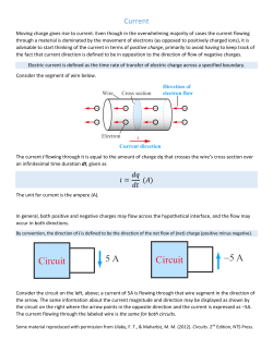


© Copyright 2026