
Workshop: Image Processing and Analysis with ImageJ
Workshop: Image Processing and Analysis with
ImageJ
Volker Baecker
Montpellier RIO Imaging
20.3.2015
2
Contents
1 Introduction
13
2 Installation and Setup of ImageJ
2.1 Installation . . . . . . . . . . . . . .
2.2 Memory and Thread Settings . . . .
2.3 Upgrading ImageJ . . . . . . . . . .
2.4 Installation of Bio-Formats . . . . .
2.5 Association of file types with ImageJ
.
.
.
.
.
.
.
.
.
.
.
.
.
.
.
.
.
.
.
.
.
.
.
.
.
.
.
.
.
.
.
.
.
.
.
.
.
.
.
.
.
.
.
.
.
.
.
.
.
.
.
.
.
.
.
.
.
.
.
.
.
.
.
.
.
.
.
.
.
.
15
15
15
16
17
17
3 A Quick Tour
3.1 The Tool-Buttons . . . . . . . . . . . . . .
3.2 The rectangular selection tool . . . . . . .
3.3 Measuring and the ImageJ Results Table .
3.4 The Selection Brush and Tool Options . .
3.5 Polygon and Freehand-Selection Tools . .
3.6 Line Selections . . . . . . . . . . . . . . .
3.7 Profile Plots . . . . . . . . . . . . . . . . .
3.8 Arrow Tool, Roi-Manager and Overlays .
3.9 Point Selections . . . . . . . . . . . . . . .
3.10 The Magic Wand Tool . . . . . . . . . . .
3.11 The Particle Analyzer . . . . . . . . . . .
3.12 Magnifying Glass and Scrolling . . . . . .
3.13 Foreground and Background Color . . . .
3.14 Macros . . . . . . . . . . . . . . . . . . . .
3.15 Macro Recorder and Batch Processing . .
3.16 Plugins . . . . . . . . . . . . . . . . . . .
3.17 Image Stacks . . . . . . . . . . . . . . . .
3.18 The ImageJ 3D Viewer . . . . . . . . . . .
.
.
.
.
.
.
.
.
.
.
.
.
.
.
.
.
.
.
.
.
.
.
.
.
.
.
.
.
.
.
.
.
.
.
.
.
.
.
.
.
.
.
.
.
.
.
.
.
.
.
.
.
.
.
.
.
.
.
.
.
.
.
.
.
.
.
.
.
.
.
.
.
.
.
.
.
.
.
.
.
.
.
.
.
.
.
.
.
.
.
.
.
.
.
.
.
.
.
.
.
.
.
.
.
.
.
.
.
.
.
.
.
.
.
.
.
.
.
.
.
.
.
.
.
.
.
.
.
.
.
.
.
.
.
.
.
.
.
.
.
.
.
.
.
.
.
.
.
.
.
.
.
.
.
.
.
.
.
.
.
.
.
.
.
.
.
.
.
.
.
.
.
.
.
.
.
.
.
.
.
.
.
.
.
.
.
.
.
.
.
.
.
.
.
.
.
.
.
.
.
.
.
.
.
.
.
.
.
.
.
.
.
.
.
.
.
.
.
.
.
.
.
.
.
.
.
.
.
.
.
.
.
.
.
19
19
20
20
21
21
22
22
24
25
25
26
27
28
28
28
30
32
32
4 Help, Documentation and Extensions
4.1 Help and Documentation . . . . . . .
4.2 Plugins . . . . . . . . . . . . . . . . .
4.3 Macros . . . . . . . . . . . . . . . . . .
4.4 Tools . . . . . . . . . . . . . . . . . . .
.
.
.
.
.
.
.
.
.
.
.
.
.
.
.
.
.
.
.
.
.
.
.
.
.
.
.
.
.
.
.
.
.
.
.
.
.
.
.
.
.
.
.
.
.
.
.
.
.
.
.
.
35
35
35
36
37
3
.
.
.
.
.
.
.
.
.
.
.
.
.
.
.
.
.
.
CONTENTS
4.5
Updating Macros and Tools . . . . . . . . . . . . . . . . . . . . .
5 Display and Image Enhancements
5.1 Brightness and Contrast Adjustment . . .
5.2 Non Linear Display Adjustments . . . . .
5.2.1 Gamma Correction . . . . . . . . .
5.2.2 Contrast Enhancement . . . . . . .
5.3 Changing the Palette - Lookup Tables . .
5.4 Overlay of Multiple Channels . . . . . . .
5.4.1 Aligning Channels . . . . . . . . .
5.4.2 Overlay of Volume Images . . . . .
5.5 Noise Suppression . . . . . . . . . . . . .
5.5.1 Convolution Filter . . . . . . . . .
5.5.2 Rank Filter . . . . . . . . . . . . .
5.5.3 Filtering in the Frequency Domain
5.6 Background Subtraction . . . . . . . . . .
5.6.1 Inhomogeneous Background . . . .
5.7 Increasing the Apparent Sharpness . . . .
.
.
.
.
.
.
.
.
.
.
.
.
.
.
.
.
.
.
.
.
.
.
.
.
.
.
.
.
.
.
.
.
.
.
.
.
.
.
.
.
.
.
.
.
.
.
.
.
.
.
.
.
.
.
.
.
.
.
.
.
.
.
.
.
.
.
.
.
.
.
.
.
.
.
.
.
.
.
.
.
.
.
.
.
.
.
.
.
.
.
.
.
.
.
.
.
.
.
.
.
.
.
.
.
.
.
.
.
.
.
.
.
.
.
.
.
.
.
.
.
.
.
.
.
.
.
.
.
.
.
.
.
.
.
.
.
.
.
.
.
.
.
.
.
.
.
.
.
.
.
.
.
.
.
.
.
.
.
.
.
.
.
.
.
.
.
.
.
.
.
.
.
.
.
.
.
.
.
.
.
38
.
.
.
.
.
.
.
.
.
.
.
.
.
.
.
41
43
45
45
48
51
53
56
57
57
60
66
67
70
72
74
6 Segmentation
6.1 Manual Threshold Selection . . . . .
6.2 Measurements and the ROI-Manager
6.3 Computed Thresholds . . . . . . . .
6.4 More than Two Object Classes . . .
6.5 Watershed Segmentation . . . . . . .
.
.
.
.
.
.
.
.
.
.
.
.
.
.
.
.
.
.
.
.
.
.
.
.
.
.
.
.
.
.
.
.
.
.
.
.
.
.
.
.
.
.
.
.
.
.
.
.
.
.
.
.
.
.
.
.
.
.
.
.
.
.
.
.
.
.
.
.
.
.
.
.
.
.
.
.
.
.
.
.
79
79
83
88
90
91
7 Image Types and Formats
7.1 Spatial resolution . . . . . . . . . .
7.2 Image types . . . . . . . . . . . . .
7.2.1 Conversion from 16 to 8 bit
7.2.2 RGB Images . . . . . . . .
7.2.3 File Formats . . . . . . . .
.
.
.
.
.
.
.
.
.
.
.
.
.
.
.
.
.
.
.
.
.
.
.
.
.
.
.
.
.
.
.
.
.
.
.
.
.
.
.
.
.
.
.
.
.
.
.
.
.
.
.
.
.
.
.
.
.
.
.
.
.
.
.
.
.
.
.
.
.
.
.
.
.
.
.
.
.
.
.
.
95
95
95
96
97
98
. . . . . . . . .
. . . . . . . . .
Automatically
not Separated .
. . . . . . . . .
. . . . . . . . .
.
.
.
.
.
.
.
.
.
.
.
.
.
.
.
.
.
.
.
.
.
.
.
.
99
. 99
. 99
. 99
. 100
. 103
. 103
.
.
.
.
.
8 Image Analysis
8.1 Counting Objects . . . . . . . . . . . . .
8.1.1 Counting Objects Manually . . .
8.1.2 Counting and Measuring Objects
8.1.3 Counting and Measuring Objects
8.2 Comparing Intensities . . . . . . . . . .
8.3 Classifying Objects . . . . . . . . . . . .
9 Annotating images
107
9.1 Scale Bar and Label Stacks . . . . . . . . . . . . . . . . . . . . . 107
9.2 Calibration Bar . . . . . . . . . . . . . . . . . . . . . . . . . . . . 109
4
CONTENTS
10 Multi-dimensional Data
10.1 Time Series . . . . . . . .
10.2 Tracking . . . . . . . . . .
10.2.1 Manual Tracking .
10.2.2 Automatic Particle
.
.
.
.
111
111
112
112
112
11 Biological Applications
11.1 Colocalization Analysis . . . . . . . . . . . . . . . . . . . . . . .
11.1.1 Visualizing Colocalization Using Overlays . . . . . . . . .
11.1.2 Quantification of colocalization . . . . . . . . . . . . . . .
115
115
115
115
. . . . . .
. . . . . .
. . . . . .
Tracking
5
.
.
.
.
.
.
.
.
.
.
.
.
.
.
.
.
.
.
.
.
.
.
.
.
.
.
.
.
.
.
.
.
.
.
.
.
.
.
.
.
.
.
.
.
.
.
.
.
.
.
.
.
.
.
.
.
.
.
.
.
CONTENTS
6
List of Figures
2.1
2.2
The memory and threads settings of ImageJ . . . . . . . . . . . .
Memory information diaplyed in the launcher window . . . . . .
16
16
3.1
3.2
3.3
3.4
3.5
3.6
3.7
3.8
3.9
3.10
3.11
3.12
3.13
3.14
3.15
3.16
3.17
3.18
Example image for chapter 3 . . . . . . . . . . . . . . . . .
Position and intensity information . . . . . . . . . . . . . .
A rectangular selection . . . . . . . . . . . . . . . . . . . . .
The ImageJ results table . . . . . . . . . . . . . . . . . . . .
Options of the selection brush . . . . . . . . . . . . . . . . .
A profile plot . . . . . . . . . . . . . . . . . . . . . . . . . .
Multiple plot profiles can be displayed in the same diagram.
An overlay . . . . . . . . . . . . . . . . . . . . . . . . . . . .
A point selection . . . . . . . . . . . . . . . . . . . . . . . .
Nuclei selected with the wand tool . . . . . . . . . . . . . .
The analyze particles dialog . . . . . . . . . . . . . . . . . .
Zoomed image with postion-indicator . . . . . . . . . . . . .
Tiff-Header information extracted by a macro . . . . . . . .
Results of the Roi Color Coder macro . . . . . . . . . . . .
The ImageJ batch processor . . . . . . . . . . . . . . . . . .
SIOX Segmentation plugin . . . . . . . . . . . . . . . . . . .
A stack of images . . . . . . . . . . . . . . . . . . . . . . . .
The ImageJ 3d viewer . . . . . . . . . . . . . . . . . . . . .
.
.
.
.
.
.
.
.
.
.
.
.
.
.
.
.
.
.
.
.
.
.
.
.
.
.
.
.
.
.
.
.
.
.
.
.
.
.
.
.
.
.
.
.
.
.
.
.
.
.
.
.
.
.
19
20
20
21
22
23
23
24
25
26
27
27
29
30
31
31
32
33
4.1
4.2
4.3
4.4
4.5
4.6
Random ovals . . . . . . . . . . . . . .
Mandelbrot fractal . . . . . . . . . . .
Selection of a tool . . . . . . . . . . .
The options of the selection brush tool
The rgb-profiles-tool . . . . . . . . . .
The macro and tool updater . . . . . .
.
.
.
.
.
.
.
.
.
.
.
.
.
.
.
.
.
.
.
.
.
.
.
.
.
.
.
.
.
.
.
.
.
.
.
.
.
.
.
.
.
.
.
.
.
.
.
.
36
37
38
38
38
39
5.1
5.2
5.3
5.4
5.5
The first example image. . . . . . . . . . . . . . . . .
Display of an image with maximum zoom . . . . . .
A matrix of intensity values. . . . . . . . . . . . . . .
Adjusting the brightness and contrast. . . . . . . . .
Adjusting the display does not change measurements
.
.
.
.
.
.
.
.
.
.
.
.
.
.
.
.
.
.
.
.
.
.
.
.
.
.
.
.
.
.
.
.
.
.
.
42
42
43
43
44
7
.
.
.
.
.
.
.
.
.
.
.
.
.
.
.
.
.
.
.
.
.
.
.
.
.
.
.
.
.
.
.
.
.
.
.
.
.
.
.
.
.
.
LIST OF FIGURES
5.6
5.7
5.8
5.9
5.10
5.11
5.12
5.13
5.14
5.15
5.16
5.17
5.18
5.19
5.20
5.21
5.22
5.23
5.24
5.25
5.26
5.27
5.28
5.29
5.30
5.31
5.32
5.33
5.34
5.35
5.36
5.37
5.38
5.39
5.40
The window and level adjuster . . . . . . . . . . . . . . . . . . .
A linear adjustment saturates high intensities . . . . . . . . . . .
The gamma function in ImageJ with different values for γ . . . .
The gamma adjustment allows to see low intensities without saturating high intensities. . . . . . . . . . . . . . . . . . . . . . . .
Selection of a toolset . . . . . . . . . . . . . . . . . . . . . . . . .
The gamma correction tool . . . . . . . . . . . . . . . . . . . . .
The enhance contrast dialog . . . . . . . . . . . . . . . . . . . . .
Histogram before and after normalization. . . . . . . . . . . . . .
The image after normalization . . . . . . . . . . . . . . . . . . .
The input image for the histogram equalization and its histogram.
The result image of the modified histogram equalization and its
histogram. . . . . . . . . . . . . . . . . . . . . . . . . . . . . . . .
The result image of the standard histogram equalization and its
histogram. . . . . . . . . . . . . . . . . . . . . . . . . . . . . . . .
The spectrum lookup-table . . . . . . . . . . . . . . . . . . . . .
The show lookup table tool . . . . . . . . . . . . . . . . . . . . .
The lookuptable in text form . . . . . . . . . . . . . . . . . . . .
An image displayed with different lookup tables. . . . . . . . . .
The HiLo lookup table . . . . . . . . . . . . . . . . . . . . . . . .
The HiLo lookup table is useful for brightness and contrast adjustments. . . . . . . . . . . . . . . . . . . . . . . . . . . . . . . .
A user created lookup table applied to an image. . . . . . . . . .
The control panel . . . . . . . . . . . . . . . . . . . . . . . . . . .
Two channels of an image. . . . . . . . . . . . . . . . . . . . . . .
The merge channels dialog . . . . . . . . . . . . . . . . . . . . . .
The overlay of two channels and the channels tool . . . . . . . .
The B&C tool automatcally works on the active channel of the
hyperstack. . . . . . . . . . . . . . . . . . . . . . . . . . . . . . .
The arrange channels dialog . . . . . . . . . . . . . . . . . . . . .
Propagation of display settings . . . . . . . . . . . . . . . . . . .
A 3d image with 3 channels . . . . . . . . . . . . . . . . . . . . .
In the image with noise values in background and object are
changed in a random manner. . . . . . . . . . . . . . . . . . . . .
The mean filter smoothes the image and reduces the impact of
the noise. . . . . . . . . . . . . . . . . . . . . . . . . . . . . . . .
The effect of the mean filter of radius one. . . . . . . . . . . . . .
Segmentation of the plant becomes possible after the application
of a mean filter. . . . . . . . . . . . . . . . . . . . . . . . . . . . .
Two populations corresponding to the object and the background
become visible after the application of the mean filter. . . . . . .
The convolver . . . . . . . . . . . . . . . . . . . . . . . . . . . . .
The image calculator . . . . . . . . . . . . . . . . . . . . . . . . .
Different representations of a convolution kernel for a gaussian
blur filter. . . . . . . . . . . . . . . . . . . . . . . . . . . . . . . .
8
45
46
46
46
47
48
48
49
49
50
50
51
51
52
52
52
53
53
54
54
55
55
56
57
58
58
59
59
60
61
61
62
62
63
64
LIST OF FIGURES
5.41 Comparison of the results of the mean filter and the Gaussian
blur filter. . . . . . . . . . . . . . . . . . . . . . . . . . . . . . . .
5.42 Comparison of the results of the mean filter and the Gaussian
blur filter on the roots image. . . . . . . . . . . . . . . . . . . . .
5.43 Plant noise image convolved with a gaussian kernel . . . . . . . .
5.44 Results of the Prewitt filter (red) displayed on the input image
(green). . . . . . . . . . . . . . . . . . . . . . . . . . . . . . . . .
5.45 Salt-and-pepper noise consisits of the addition of white and black
pixels to the image. . . . . . . . . . . . . . . . . . . . . . . . . . .
5.46 Comparison of the results of the median and the mean filter on
salt-and-pepper-noise. . . . . . . . . . . . . . . . . . . . . . . . .
5.47 An image and its power spectrum calculated with the FFT. . . .
5.48 Filtering frequencies in the power spectrum . . . . . . . . . . . .
5.49 The window blinds have disappeared in the filtered image. . . . .
5.50 The suppressed frequencies . . . . . . . . . . . . . . . . . . . . .
5.51 Letting only low frequencies pass smoothes the image. . . . . . .
5.52 Letting only high frequencies pass can be used to enhance edges.
5.53 The bandpass filter suppresses high and low frequencies. . . . . .
5.54 A bandpass filter can correct the inhomogenous background. . .
5.55 A profile plot before and after the application of the bandpass
filter. . . . . . . . . . . . . . . . . . . . . . . . . . . . . . . . . . .
5.56 The mean background is above zero. . . . . . . . . . . . . . . . .
5.57 The image after the subtraction of the mean background intensity.
5.58 Subtracting a constant does not help if the background is inhomogenous. . . . . . . . . . . . . . . . . . . . . . . . . . . . . . . .
5.59 The subtract background command removes the gradient using
a rolling ball algorithm. . . . . . . . . . . . . . . . . . . . . . . .
5.60 The gradient is present in the generated background and not in
the result of the pseudo flatfield correction. . . . . . . . . . . . .
5.61 The unsharp mask filter increases the apparent sharpness. . . . .
6.1
6.2
Different display modes of the threshold adjuster. . . . . . . . . .
The wand tool allows to select connected pixels. It works in
combination with the threshold adjuster. . . . . . . . . . . . . . .
6.3 The particle analyzer . . . . . . . . . . . . . . . . . . . . . . . . .
6.4 Two ways to represent image objects with the particle analyzer .
6.5 The set measurements dialog . . . . . . . . . . . . . . . . . . . .
6.6 The outlines of the objects found by the particle analyzer, the in
the image, the objects in the roi-manager and the measurements
of the objects in the results table. . . . . . . . . . . . . . . . . . .
6.7 The skewness is a measure of the asymmetry of the distribution.
6.8 Distributions with different kurtosis values. . . . . . . . . . . . .
6.9 Global auto-thresholding methods applied to the plant image . .
6.10 Global auto-thresholding methods applied to the root image . . .
6.11 Local auto-thresholding methods applied to the plant image . . .
6.12 Local auto-thresholding methods applied to the root image . . .
9
64
65
65
66
67
68
69
70
70
71
71
72
72
73
73
74
74
75
75
76
77
80
81
81
82
82
84
86
87
88
89
89
90
LIST OF FIGURES
6.13 Image segmented into four classes . . . . . . . . . . . . . . . . . .
6.14 Separation of objects with a binary watershed algorithm. . . . .
6.15 The watershed interprets the distance map as a landscape that
is filled with water step by step. . . . . . . . . . . . . . . . . . . .
6.16 Watershed dams . . . . . . . . . . . . . . . . . . . . . . . . . . .
7.1
7.2
7.3
7.4
8.1
8.2
8.3
8.4
8.5
8.6
8.7
8.8
8.9
9.1
9.2
9.3
The conversion from 16 to 8 bit scales from the min. and max.
display values to 0 and 255. . . . . . . . . . . . . . . . . . . . . .
The RGB profile plot consists of a plot for each channel of the
RGB image in the same diagram. . . . . . . . . . . . . . . . . . .
RGB and HSB channels. . . . . . . . . . . . . . . . . . . . . . . .
Green and red mix to yellow . . . . . . . . . . . . . . . . . . . . .
91
92
92
93
96
97
98
98
The cell counter helps to count multiple classes of objects in an
image. . . . . . . . . . . . . . . . . . . . . . . . . . . . . . . . . . 100
The particle analyzer allows to count and measure objects automatically. . . . . . . . . . . . . . . . . . . . . . . . . . . . . . . . 101
The outlines of the objects and the summary of the measurements.101
Local thresholding helps to spearate objects touching each other. 102
Segmentation with the watershed algorithm . . . . . . . . . . . . 103
Measuring intensities in nuclei and cytoplasm . . . . . . . . . . . 104
Separating two classes of objects . . . . . . . . . . . . . . . . . . 104
Features based on moments . . . . . . . . . . . . . . . . . . . . . 105
Features based on moments . . . . . . . . . . . . . . . . . . . . . 105
9.4
Setting the scale by indicating a known distance. . . . . . . . . .
Adding a scale bar to each frame of the time series. . . . . . . . .
The time series with a scalebar and a time label in each frame
and an event label in some frames . . . . . . . . . . . . . . . . .
An image with a calibration bar . . . . . . . . . . . . . . . . . .
109
110
10.1
10.2
10.3
10.4
The stack tools toolset . . . . . . . . . . . . . . . . . . .
Basic manual tracking with the point-tool . . . . . . . .
The plugin MTrackJ provides tools for manual tracking.
Automatic tracking with the MTrack2 plugin. . . . . . .
111
113
113
114
.
.
.
.
.
.
.
.
.
.
.
.
.
.
.
.
.
.
.
.
11.1 Different overlays of the two channels before and after histogram
normalization. . . . . . . . . . . . . . . . . . . . . . . . . . . . . .
11.2 The points form a tight cloud around a line with a positive slope
which indicates a high correlation. . . . . . . . . . . . . . . . . .
11.3 The points do not form a cloud which indicates that the two
images are not correlated. . . . . . . . . . . . . . . . . . . . . . .
11.4 The points form a tight cloud around a line with a negative slope
which indicates a high anti-correlation. . . . . . . . . . . . . . . .
11.5 Pearson’s coefficients for different scatter plots . . . . . . . . . .
11.6 The dialog of the Coloc 2 plugin . . . . . . . . . . . . . . . . . .
10
108
108
116
117
117
118
118
119
LIST OF FIGURES
11.7 Scatter plot and overlay of the channels. . . . . . . . . . . . . . . 119
11
LIST OF FIGURES
12
Chapter 1
Introduction
In this workshop you will learn how to apply image analysis and processing
techniques, using the public domain software ImageJ[8] and some additions
(plugins and macros). ImageJ has been written and is maintained by Wayne
Rasband at the National Institute of Mental Health, Bethesda, Maryland, USA.
ImageJ is the successor of the Macintosh software NIH Image[31] written by
Wayne Rasband. ImageJ is written in Java, which means that it can be run
on any system for which a java runtime environment (jre) exists. It can be run
under Windows, Mac, Linux and other systems. It can be run as a java applet
on a website or as a standalone application.
Because of the easy way in which ImageJ can be extended, using macros
and plugins, a lot of functionality is available today, especially in the fields of
microscopy and biology.
13
CHAPTER 1. INTRODUCTION
14
Chapter 2
Installation and Setup of
ImageJ
2.1
Installation
The ImageJ homepage is http://imagej.nih.gov/ij/. Go to the download
page and download the appropriate version for your operating system. In this
workshop we will only use windows. For windows there are three versions available:
• ImageJ bundled with a 32-bit java runtime environment
• ImageJ bundled with a 64-bit java runtime environment
• ImageJ without a java runtime environment
To use the last version, the java runtime environment must already be installed
on your computer. For this tutorial we download the ImageJ bundle with the
64-bit java included. Run the installer and follow the instructions on the screen.
The first time ImageJ is started, a configuration file for your installation will be
created.
The installer will create a quick-start icon and a desktop icon. You can use
these to start ImageJ. You can open images by dropping them onto the desktop
icon.
2.2
Memory and Thread Settings
Java applications will only use the memory allocated to them. Under Edit>Options>Memory
& Threads... you can configure the memory available to ImageJ (fig. 2.1).
The maximum memory should be set to 3/4 of the available memory on your
machine. To find out how much memory your machine has, open the properties
of My Computer and look for the amount of available RAM. The number of
15
CHAPTER 2. INSTALLATION AND SETUP OF IMAGEJ
Figure 2.1: The memory and threads settings of ImageJ.
parallel threads for stacks is by default set to the number of processors or cores
available in your system.
A dialog tells you that the change will be applied the next time you start
ImageJ. The configuration is stored in the file ImageJ.cfg in the ImageJ folder.
Should ImageJ not start after you changed the memory settings, delete the file
ImageJ.cfg, restart ImageJ and set the maximum memory to a lower value.
A double-click on the lower part of the ImageJ launcher window displays the
amount of used and available memory (fig. 2.2).
Figure 2.2: A double click on the window displays memory information.
You can use Plugins>Utilities>Monitor Memory... to monitor the memory usage.
2.3
Upgrading ImageJ
To upgrade ImageJ, start ImageJ and go to Help>Update ImageJ.... Select
the latest version from the list. ImageJ will be closed. Open it again and look at
Help>About ImageJ... to see the current version number. Alternatively you
can download the latest pre-release version of ImageJ from http://imagej.
nih.gov/ij/upgrade/. Download the file ij.jar and replace the version in
the ImageJ home folder with the new version.
16
2.4. INSTALLATION OF BIO-FORMATS
2.4
Installation of Bio-Formats
ImageJ can read a number of image formats like tiff (and tiff stacks), dicom,
fits, pgm, jpeg, bmp or gif images. It can not read other formats like ics or lsm
by itself. If you want to work with these file formats you need plugins that can
handle them.
Bio-Formats[17] is a project that implements a library which can read many
biological image formats.
“Bio-Formats is a standalone Java library for reading and writing
life sciences image file formats. It is capable of parsing both pixels
and metadata for a large number of formats, as well as writing to
several formats”.1
ImageJ can take advantage of the bioformats library. You only have to download the file loci tools.jar from http://www.loci.wisc.edu/bio-formats/
downloads and to put it into the plugins folder of your ImageJ installation. ImageJ will automatically use it when it can not open an image itself. The easiest
way to install the plugin is to drag the link to the jar file directly from the
website onto the ImageJ launcher window. This will download the plugin and
ask you where under the plugins folder you want to save it. In this case you can
save it directly into the plugins folder.
2.5
Association of file types with ImageJ
To open images by double-clicking we have to associate the file type with the ImageJ program. Download the zip-archive of example images (images.zip) from
the mri wiki http://dev.mri.cnrs.fr/wiki/imagej-workshop and unzip the
archive.
Right-click on a tif-image, select ‘‘open with’’ and ‘‘choose the program’’
from the context menu. On the dialog click the browse button and select
ImageJ.exe from the ImageJ home directory. Check the ‘‘always use this
program to open files of this type’’ option and click ok on the dialog.
In the same way associate jpg-images with ImageJ. If on recent versions of
windows you have problems to associate ImageJ with file-types, download and
double-click the file imagej.reg from the resources-folder of the page http:
//dev.mri.cnrs.fr/projects/list_files/imagej-workshop. This will add
some information about ImageJ to the registry.
If for each image you open a new ImageJ instance is started, go to the menu
Edit>Options>Misc... and select the ‘‘Run single instance listener’’
checkbox. Instead of running a new ImageJ for each image, all images will now
be opened in the same Image instance.
1 from
http://loci.wisc.edu/software/bio-formats
17
CHAPTER 2. INSTALLATION AND SETUP OF IMAGEJ
18
Chapter 3
A Quick Tour
Before explaining the image analysis tools in ImageJ in more detail, we will make
a quick tour to get an overview of the most important tools. We will use the
images you downloaded in section 2.5. Open the image A4 dapi 1.tif. You
can drag an image from your operating system browser to the ImageJ window
to open it. We will use this image for all examples in chapter 3.
Figure 3.1: The example image for chapter 3.
Move the mouse-pointer over the image and watch the ImageJ window. The
position of the mouse-pointer and the intensity at that position are displayed in
the lower part of the window (fig. 3.2). If it is difficult to see the mouse over the
image, you have probably the crosshair cursor activated. You can switch back
to a pointer cursor in the menu Edit>Options>Misc....
3.1
The Tool-Buttons
Now look at the tool-buttons in the ImageJ window. The twelve tools upto the
color picker are basic tools that are always displayed. The tools on the remaining
19
CHAPTER 3. A QUICK TOUR
Figure 3.2: The position and intensity are displayed in the launcher window.
buttons can be changed. The rightmost button allows to select a tool-set that
puts tools on these buttons. The first section in the drop-down-menu contains
complete tool-sets. The following sections allow to add a single tool to the next
free button or to replace the tool on the last button if no free button remains.
This way you can setup your own tool-sets that are remembered by ImageJ. Try
this and when you finished call Restore Startup Tools to reset the tools.
When you click on a tool button the button remains pressed and the corresponding tool will be active until you press another tool button. Notice that
the name of the tool is displayed when the mouse pointer is over a tool button.
3.2
The rectangular selection tool
Make sure that the rectangular selection tool is active. You can now make a
rectangular selection in the image by clicking at a point and dragging the mouse.
While doing this the width, the height and the aspect ratio of the selection are
displayed. Once you release the mouse button you made a selection on the
image. You can still change its position by clicking into it and dragging and its
size by using the handles.
Figure 3.3: A rectangular selection.
3.3
Measuring and the ImageJ Results Table
Try to make a selection that contains exactly one nucleus. Then press the key
m on the keyboard. This is the shortcut for the measure command that can be
20
3.4. THE SELECTION BRUSH AND TOOL OPTIONS
found in the Analyze menu. The ImageJ results table (fig. 3.4) will be opened.
The table contains the results of the measurements. All measurements will be
stored in this global table. In the File menu you have the possibility to duplicate the table to keep measurements. From the Results menu you can remove
everything from the system table with the command Clear Results. The Set
Measurements command allows to define which properties will be measured.
Note that the change will only be active for future measurements, the corresponding columns for already existing measurements will be filled with zero
values.
Figure 3.4: The ImageJ results table.
3.4
The Selection Brush and Tool Options
Behind tool buttons that have a small, red triangle in the lower right corner,
you can find a list of tools by right-clicking on the button. Remove all selections
from the image. You can do this by clicking somewhere in the image while the
rectangular selection tool is active or by pressing shift a (a is the shortcut for
select all, shift-a for select none from the menu Edit>Selection). Right-click
on the elliptical-selection tool button and select the selection brush tool.
Click in the image and move the mouse, keeping the button down. You can
paint a selection onto the image. Once you released the button, you can add to
the selection by holding down the shift key while painting. You can remove
from a selection by holding down the alt key. These two modifier keys work
for all kinds of selections in ImageJ. Note that on some systems you have to use
ctrl+alt instead of alt, since the operating system is using the modifier key
itself.
Tools can have options. You can access them by double-clicking on the tool
button. Change the size of the brush used by the selection brush tool (fig. 3.5).
3.5
Polygon and Freehand-Selection Tools
Try the polygon and freehand-selection tools. Note that you do not have to close
the selections at the end. For the polygon selection you can finish the process
by right clicking and the selection will automatically be closed. The freehand
selection will be closed as soon as you release the mouse button.
21
CHAPTER 3. A QUICK TOUR
Figure 3.5: The options of the selection brush tool.
3.6
Line Selections
The line selection tools: straight line, segmented line and freehand line
can be used to measure lengths. Besides the length the straight line tool measures the angle with the horizontal x-axis. Use a right click to finish a segmented line. The angle tool can be used to measure arbitrary angles. The
line tools have the line width as a parameter. If the line width is bigger than
one, the pixels within the line width will be taken into account for some measurements and operations. A line selection can be transformed into an area
selection and vice versa using the commands Edit>Selection>Line to Area
and Edit>Selection>Area to Line.
3.7
Profile Plots
You can use the line selection tools to create profile plots. First make a line
selection across a nucleus, then press the key k (the shortcut for Analyze>Plot
Profile). Note that, when the line width is bigger than one, the profile will be
averaged over the width.
If you want averaged line profiles of horizontal or vertical lines, you can use
the rectangular selection tool instead. If you want to use vertical lines you have
to press alt-k instead of k.
A profile plot can be used to measure properties like, for example, the diameter of an object by taking into account only intensity values above a baseline,
that is visible in the plot. Note that the plot is an image itself and that you
can make selections on it and measure them. Furthermore the plot-image has
a spacial calibration that corresponds to the values displayed on the axis of the
diagram. This allows to measure values corresponding to the image from which
the plot has been created, independent of the size of the selection that was used
to create it.
Press the Live button on the profile plot window (fig. 3.6) and move the
line-selection across the image or modify it. The profile plot is now updated as
the line selection changes. Press the Live button again to switch the live-mode
off.
22
3.7. PROFILE PLOTS
Figure 3.6: A profile plot along a line crossing a nucleus.
It is possible to display multiple profile plots in the same diagram. You
can do this by adding the line selections to the roi-manager. You can open the
roi-manager from Analyze>Tools>ROI Manager... and use the Add button to
add the selection or by using the keyboard shortcut t. After you added multiple
selections to the roi-manager select More>Multi Plot from the roi-manager to
create the plot. Note that this works as well on different slices of a stack and
on different channels of a hyperstack.
(a) Multiple line-selection in the (b) Multiple profile plots in the same diaroi-manager for the creation of a gram.
profile plot.
Figure 3.7: Multiple plot profiles can be displayed in the same diagram.
23
CHAPTER 3. A QUICK TOUR
3.8
Arrow Tool, Roi-Manager and Overlays
Select the arrow tool from the straight line tool button. Double click to
open the options dialog and set magenta as foreground color. Click in the image
and drag the mouse to create an arrow. With the shift modifier key you can
restrain the arrows to horizontal and vertical ones.
If you want to have multiple arrows you can add them to the overlay by
pressing the b key (shortcut for Image>Overlay>Add Selection). You can use
the text tool to add an annotation to an arrow. Use ctrl+alt+b to add it to
the overlay as well.
Figure 3.8: A non-destructive overlay of arrows and annotations on the image.
If you want to be able to modify objects in the overlay, you have to add
them to the roi-manager. Roi stands for region of interest and the roi-manager
is the tool that allows to manage multiple selections. Use Image>Overlay>To
ROI Manager to add the objects in the overlay to the roi-manager. Note that
you find the roi-manager under Analyze>Tools. Make sure that Show All and
Edit Mode are selected. You can now select a selection object by clicking on
its number in the image or by selecting it in the list in the roi-manager. You
can modify the selected selection object and make the change permanent by
pressing update on the roi-manager. To create an rgb-snapshot of your image
with overlay use the flatten command from the roi-manager. Note that overlay
and roi-manager can be used with all kinds of selection, not only arrows and
text.
Delete all overlays and all seletions in the roi-manager. Make some area
selections on the image and add each to the roi-manager. Make sure that no
roi is selected and press the measure button. Each selection will be measured
independently.
24
3.9. POINT SELECTIONS
3.9
Point Selections
You can use the point selection tools to manually count objects in an image
(fig. 3.9). With the point selection tool use shift to add points. You can
delete points using alt. Note that the numbers of the remaining points change
accordingly. If you make an error and you loose your selection you can get the
last selection back using shift+e (the shortcut for Edit>Selection>Restore
Selection). You can add the selection to the roi-manager or measure it. The
options allow to directly add each point to the manager or to measure it while
you are working. If you use the multi-point selection tool, you do not have
to use shift to add points, so you are less likely to accidentally delete the
selection. As before you can use flatten on the roi-manager to create an image
that permanently contains the point markers. Using the more button on the
roi-manager you can save and load selections, in case you need a break in the
middle of counting.
Figure 3.9: Counting objects with the point selection tool.
3.10
The Magic Wand Tool
Use the wand tool to select all nuclei, one after the other. Add them to the roimanager and measure them. To do this you either need to change the tolerance
25
CHAPTER 3. A QUICK TOUR
in the wand tool’s options or you need to set a threshold on the image. If a
threshold is set on the image the wand tool selects all connected pixel above the
lower and below the upper threshold value. To define a threshold value press
shift-t (the shortcut for Image>Adjust>Threshold) to open the threshold
tool. Select Dark background. If you select the Over/Under mode in the right
selection box, values below the lower threshold will be displayed in blue and
values above the upper threshold will be displayed in green. Adjust the lower
threshold and select the nuclei using the wand tool (fig. 3.10).
Figure 3.10: A lower threshold is set and the nuclei have been selected using
the wand tool.
3.11
The Particle Analyzer
Instead of clicking on each object with the wand tool, you can let the particle
analyzer do the work. As before, define the lower threshold, then call Analyze
Particles from the menu Analyze. Make sure that only Add to Manager is
selected in the Analyze Particles dialog (fig. 6.4). Then click ok. You can
exclude too small or too big objects by supplying a minimal and maximal size
in the Particle Analyzer dialog.
26
3.12. MAGNIFYING GLASS AND SCROLLING
Figure 3.11: The analyze particles dialog.
3.12
Magnifying Glass and Scrolling
The magnifying glass tool allows to change the zoom of the image. A left click
zooms in and a right click zooms out. When the image is bigger than the window
the position of the current view is indicated in the upper left corner (fig. 3.12).
The scrolling tool allows to move the image in the window by clicking and
dragging. The keyboard shortcuts for zooming are + and and the scrolling can
be done by holding down space. Scrolling with the space key down allows to
scroll while another tool is active.
Figure 3.12: The position of the current view in the image is indicated.
27
CHAPTER 3. A QUICK TOUR
3.13
Foreground and Background Color
The color picker allows to select the foreground color from an image. Select the
tool and click somewhere in the image. The foreground color will be changed.
In the options of the color picker the background and foreground colors can be
swapped and the colors can be selected from a palette. Note however that only
gray-scale values will be used as long as the image is not a color image. You
can use Image>Type>RGB Color to convert the image into a color image. The
foreground color will be used by the commands Fill and Draw from the menu
Edit and the background color will be used by the commands Clear and Clear
Outside. After you have changed your image you can reload the original version
from disk by pressing the r key (shortcut for File->Revert).
3.14
Macros
Macros are small programs written either in the ImageJ macro language or in
a scripting language, that can be run by ImageJ to automate image analysis
tasks. Click on the dev menu button of the Startup Tools and select Macros.
This will open a list of macros on the ImageJ website. Search the macro with
the name DisplayTiffInfo.txt. Drag the link from the web-page and drop
it onto the ImageJ launcher window. This will open the macro in the ImageJ
macro editor. You can run it using the command Run Macro from the menu
Macros of the macro editor. This macro will display some information stored
in the header of the image (fig. 3.13).
We will try another macro. The macro ROI Color Coder.ijm can mark
objects with a color according to the value of a given property, for example area
or roundness. Open the macro by dropping it on the ImageJ launcher window.
To use the macro we need the selections of the objects in the roi-manager and
the corresponding measurements in the results table. Set the threshold and
use the Particle Analyzer and the measure command from the roi-manager to
achieve this, then run the macro. If the color code looks strange, make sure
that you reset the line width of the line selection tool to 1.
3.15
Macro Recorder and Batch Processing
Imagine we want to measure some properties like size and form of the nuclei in
our image, but in many images, not only in one. We could run all the commands
needed on each image, one after the other to achieve this. But we can do better:
We can record the commands needed to analyze one image and create a macro
from them.
Start the macro recorder under Plugins>Macros>Record.... Under Analyze>Set
Measurements select the properties you want to measure. Make sure that
centroid is among the selected measurements, it will be needed later for the
label command. Now set the threshold and run the particle analyzer. In the
particle analyzer select Display results only. Then run Analyze>Label. Do
28
3.15. MACRO RECORDER AND BATCH PROCESSING
Figure 3.13: The macro displays information from the tiff-header of the image
file.
not worry about the message. It appears because the label command has to different modes, one for labelling active rois interactively and one for labelling rois
with the information from the results table, when running from a macro. Close
the message dialog. Remove unneeded commands from the macro recorder,
then click Create and close the recorder window. You should now have a macro
similar to the following:
run("Set Measurements...", "area mean standard modal min
centroid center perimeter display redirect=None decimal=3");
setAutoThreshold("Default dark");
run("Analyze Particles...", "size=10-Infinity
circularity=0.00-1.00 show=Nothing display");
run("Label");
Open the first image from the folder 13-batch and run the macro. Press
shift-o (the shortcut for File>Open Next) to open the next image in the folder
and run the macro again. Repeat this until all images are analyzed.
Of course we can still do better. We do not have to load each image manually.
Copy the text of the macro, then open Process>Batch>Macro and paste it into
the text part of the dialog (fig. 3.15). Select the input folder. Create a new
folder and select it as result folder, then press the Process button. As a result
you will get the measurements in the results table and the labeled images in the
results folder.
29
CHAPTER 3. A QUICK TOUR
(a) The roundness of the objects is marked with a color-code. (b) The color
code for the
roundness in the
left image.
Figure 3.14: Results of the Roi Color Coder macro
3.16
Plugins
Plugins are java modules that can be used to add functionality to ImageJ. A
large number of plugins concerning microscopy is available. Select Plugins from
the Dev menu button. This will open the plugins page on the ImageJ website
in your browser. Look for the SIOX[10] (Simple Interactive Object Extraction)
plugin and click on the link. This plugin will allow to segment color images by
giving examples of background and foreground areas. To install the plugin drag
the siox .jar link from the webpage and drop it onto the ImageJ launcher window. A file-save dialog will pop-up. Use it to create a subfolder Segmentation
of the folder plugins and save the plugin into this subfolder. It will now be
available in the Plugins menu in ImageJ.
Open one of the images from the 04 plant (roboter) folder. Run the
siox-plugin from the plugins menu. Use a selection tool and select multiple
foreground zones holding down the shift key. Then switch to background and
select multiple background zones (fig. 3.16). Press the segment button. If you
want you can create a mask for further processing.
30
3.16. PLUGINS
Figure 3.15: The ImageJ batch processor.
Figure 3.16: SIOX Segmentation plugin.
31
CHAPTER 3. A QUICK TOUR
3.17
Image Stacks
Stacks can either represent volume data or time series. Open the example stack
T1 Head from the Stk menu button. Note the slider below the image. You can
use it to select the visible slice of the stack.
Figure 3.17: A stack of images in ImageJ.
The play and pause button next to the slider allow to start and stop the
animation of the stack. A right click on the same button opens the optionsdialog for the animation. Try the commands z project, 3d-project and make
montage. Combine allows to combine to stacks one next to the other or one
above the other, while Concatenate allows to add the slices of one stack at the
end of another.
3.18
The ImageJ 3D Viewer
Close all ImageJ windows and open the T1 Head stack again. Run the 3D
viewer[30] from the menu Plugins>3D>3D Viewer. On the Add Content dialog
press the ok button. A dialog will ask if you want to convert the image to 8-bit
so that it can be used with the 3D viewer. Answer the dialog with ok. You now
added the stack to the 3D viewer (fig. 3.18).
As long as the scrolling tool is selected you can turn the 3d scene by dragging
with the mouse. Make a freehand-selection that covers a part of the head in
the 3D-scene. Now right-click to open the context menu and run the command
Fill Selection. Reselect the scrolling tool and turn the head so that you can
see the area that you cut.
32
3.18. THE IMAGEJ 3D VIEWER
Figure 3.18: A 3d scene. Part of the data has been cut-off with the fill command.
33
CHAPTER 3. A QUICK TOUR
34
Chapter 4
Help, Documentation and
Extensions
4.1
Help and Documentation
At the page http://imagej.nih.gov/ij/docs/ you can find help for the menu
commands in the ImageJ User Guide written by Tiago Ferreira and Wayne Rasband. The page can be accessed from within ImageJ via the menu Help>Documentation....
In the tutorials section you can find a link to the EMBL/CMCI ImageJ Course
Textbooks as well as a link to this workshop ImageJ Workshop (manuscript,
slides and exercises).
Further information can be found at the ImageJ Documentation Wiki: http:
//imagejdocu.tudor.lu/doku.php.
The book “Digital Image Processing An Algorithmic Introduction using
Java”[6] can be found here: http://www.imagingbook.com/index.php.
A very short and basic introduction to ImageJ is given in the book “Image
Processing with ImageJ”[26] that can be bought here: https://www.packtpub.
com/application-development/image-processing-imagej.
You can find more detailed explanation of some image processing techniques
in the hyperlink image processing ressource (hipr) at: http://homepages.inf.
ed.ac.uk/rbf/HIPR2/index.htm.
4.2
Plugins
New functions can be added to ImageJ by installing plugins. Plugins either add
commands to some menus or they can be run from the Plugins menu and its
sub-menus once they have been installed.
You can access the ImageJ plugin-site from the menu Help>Plugins.... If
the plugin is available as a .jar or a .class file, you can install it by dragging
the link directly from your web-browser onto the ImageJ launcher window. This
35
CHAPTER 4. HELP, DOCUMENTATION AND EXTENSIONS
will cause ImageJ to download the plugin. It then opens a dialog that lets you
copy the plugin into the plugins folder or into one of its sub-folders.
Should the plugin come as a zip file, unzip it into a temporary folder. If
the content consists of .jar or .class files, you can drag them to the ImageJ
launcher window in the same way as described above to install them. Otherwise
follow the instructions on the web-site from which you downloaded the plugin.
As an example we will install a plugin that draws random ovals into a
new image. Use the help menu to go to the plugin site. Scroll down to
the category “Graphics” and click on the link Random Ovals. Drag the link
Random Ovals.class onto the ImageJ launcher window. Select the folder Graphics
in the Save Plugin... dialog or create it if it doesn’t exist. You can now directly run the newly installed plugin from the Plugins menu, using Plugins>Graphics>Random
Ovals.
Figure 4.1: The result of the “Random Ovals” plugin.
4.3
Macros
Macros are scripts in the ImageJ-macro language. A number of macros is available in the folder macros in the ImageJ base-folder. You can open them by dragging them onto the ImageJ launcher window or by using Plugins>Macros>Edit....
You can access the ImageJ macro site from the menu Help>Macros. You can
directly drag a link to a macro from the web-browser onto the ImageJ launcher
window. This will open the macro in the ImageJ macro editor, from which you
can run the macro using the menu Macros>Run Macro (or ctrl+r). Try to run
the macro Mandelbrot.txt this way.
36
4.4. TOOLS
Figure 4.2: The result of the Mandelbrot macro.
4.4
Tools
Tools are macros that add a tool button to ImageJ’s toolbar. Note that the
name of the tool is displayed in the status line, when you move the mouse over
a tool button. There is a difference between action tools and tools. Action tools
execute a single command. They do not change the active tool. When you press
the button of a tool, that is not an action tool, you change the active tool. The
active tool will usually do something when you click in an image. An example
of a tool is the Rectangular Selection tool. An example of an action tool is
Next Slice from the Stack Tools toolset. You can try it with the MRI Stack
from the Stk menu button on the same toolset.
There can be multiple tools hidden behind one tool-button. If this is the
case a small red arrow is displayed on the button. A right-click on the button
shows the list of tools and allows to change the tool. Look for example at the
second button from the left. This is the Oval selections tool. A right-click on
the button gives access to the Elliptical selections tool and the Selection
Brush Tool (fig. 4.3).
A tool or a group of tools (those that share the same button) can have
options. The options can be accessed by a double-click on the tool button.
Select Macros from the menu Help. On the web-page scroll down to the
tools folder and enter into it. Search for RGBProfilesTool.txt and drag the
link onto the ImageJ toolbar. The first free tool-button will become the button
for the rgb profiles tool. If there is no free tool-button the last tool is replaced
with the rgb profiles tool. You can call Remove Custom Tools from the >>
button to start with an empty toolbar. Run Macros>Install Macros from the
macro editor to reinstall the tool on the empty bar.
37
CHAPTER 4. HELP, DOCUMENTATION AND EXTENSIONS
Figure 4.3: A right click allows to select between different tools.
Figure 4.4: The options of the selection brush tool.
Open the image clown.jpg from File>Open Samples>Clown and try the
rgb-profiles-tool.
(a) An rgb example image.
(b) The rgb profile along the line
in the image.
Figure 4.5: The rgb-profiles-tool
4.5
Updating Macros and Tools
There is a tool available that automatically downloads and updates the macros
and tools from the ImageJ website to your local machine. Get the toolset
Luts Macros and Tools Updater from the folder toolsets on the macros page
38
4.5. UPDATING MACROS AND TOOLS
(Help>Macros). Save it into the local folder macros/toolsets of your ImageJ
installation. Now click on the leftmost menu-button of the toolset and select
Macro, Tools and Toolsets Updater. Then answer the questions in the dialog.
Figure 4.6: The macro and tool updater.
New macros, tools and toolsets will be downloaded into the ImageJ/macros,
the ImageJ/macros/tools and the ImageJ/macros/toolsets folders. Existing
macros, tools and toolsets will be updated if a newer version is available on the
website.
39
CHAPTER 4. HELP, DOCUMENTATION AND EXTENSIONS
40
Chapter 5
Display and Image
Enhancements
Before we start to work on images we should answer a simple question: “What
is a digital image?”. There are different kinds of images, of course. Images can
for example be two or three dimensional and they can have one or more color
channels.
An image is a rectilinear array of point samples (pixels). The word pixel
is build from “pix element”. Pix is an abbreviation for picture [18]. In the
simplest case the array has two dimensions and width × height pixels. The
distance between the point samples is sometimes called the pixel size. The pixel
consists of the coordinates in the image and an associated sample value. The
sample value can be an integer between 0 and a maximum value. The sample
values can be interpreted as intensities. 0 usually means no intensity, yielding
a black pixel. Higher values usually mean lighter pixels and lower values mean
darker pixels.
When a digital image is displayed on a device the elements of the image
must be mapped to the elements of the output device. This can be done in
different ways. One way is to let each output element display the sample value
of the nearest existing image sample. This results in pixels being displayed as
little squares. Better results can be achieved by using interpolated values for
the output elements.
Open the image example1.tif. You can either double click the image or
use File>Open from the ImageJ window. When an ImageJ window is active
you can use keyboard shortcuts to call commands from the ImageJ menus. To
get the open dialog, click on an ImageJ window and press ‘o’.
Use the magnifying glass tool and click multiple times on the image to get
the maximum zoom. You can now see the individual pixels being displayed
as little squares (fig. 5.2). Select Interpolate Zoomed Images in the menu
Edit>Options>Appearance to switch to an interpolated display.
The coordinates and the intensity value of the pixel under the mouse pointer
41
CHAPTER 5. DISPLAY AND IMAGE ENHANCEMENTS
Figure 5.1: The first example image.
Figure 5.2: With a higher zoom, individual pixels become visible as little
squares.
are displayed at the bottom of the ImageJ window. You can use the right mouse
button to zoom out again. To scroll the image hold down space-bar, press the
left mouse button and move the mouse. Remark that the origin of the coordinate
system is in the upper left corner of the image with increasing coordinates from
left to right and top to bottom.
Save the image as a text image to the desktop and open it with a text editor
or drop it on the ImageJ window. You see the image as a matrix of intensity
values (fig. 5.3).
42
5.1. BRIGHTNESS AND CONTRAST ADJUSTMENT
Figure 5.3: The image as a matrix of intensity values.
5.1
Brightness and Contrast Adjustment
Open the image bc-adjust.tif. The image is dark and the contrast is very low.
Open the Brightness and Contrast Adjuster from the menu Image>Adjust>Brightness/Contrast
or press shift+c.
(a) The intensi- (b) The bright- (c) The image
ties are too low ness and contrast after the autoto distinguish de- adjuster.
adjustment.
tails in the image.
(d) After the adjustment intensities below 3 will
be displayed as
black and intensities above 26 as
white.
Figure 5.4: Adjusting the brightness and contrast.
Press the Auto button to make an automatic adjustment. With Reset you
can go back to the original display. Use the four sliders to adjust brightness
and contrast manually. Remark that only the displayed intensities are changed,
the pixel values remain unchanged. Call Analyse>Measure or select the image
43
CHAPTER 5. DISPLAY AND IMAGE ENHANCEMENTS
and press m, then change the brightness/contrast and measure again. Compare
the values mean and IntDen, which give the average and total intensity in the
image. If you cant find mean or IntDen in the results table, open the dialog
Analyze>Set Measurements... and check Mean Gray Value and Integrated
Density.
Figure 5.5: Adjusting the display does not change measurements.
The Integrated Density takes into account a calibration of the intensity
values that can be set under Analyze>Calibrate.... The Raw Integrated
Density is always calculated from the raw intensity values in the image.
How does the adjustment work? When the image is displayed two points
are stored together with the image. The point (min, 0) and the point (max,
maxIntensity). All intensity values below min are displayed with the intensity
zero, all intensity values above max will be displayed with the intensity value
maxIntensity. Values between min and max are mapped by the line equation
that is defined by the two points (min,0) and (max, maxIntensity).
In the beginning when we opened the example image, min was 0 and max was
255 and the maxIntensity is 255. Since this defines a line with the gradient 1,
each intensity value is mapped to itself. After we applied the auto adjustment,
min becomes 2 and max 27, so pixels that have the intensity 27 are displayed
with the value 255, pixels that have the intensity 20 with the value 184, and so
on.
Now look at the image in the upper part of the B&C window. What you
see there is the histogram of the image. On the x-axis are the intensity values
from 0 to 255. On the y-axis you find the count of pixels in the image that
have the intensity x. We will come back to the histogram later when we talk
about thresholding. For the brightness and contrast adjustment it shows you
how many pixels you set to the max. intensity and to zero. On the left you find
the min. display value and on the right the max. display value. The line that is
drawn in the histogram shows the mapping of the values between min and max.
If you move the brightness slider to the right the whole line will move to the
left and lower intensity values will be mapped to higher display values, making
the display brighter. If you move the contrast slider to the right the gradient
of the line increases so the intensity values closer together will be mapped to
display values with a bigger distance. You can use the set button to enter the
min and max value directly. If you press apply, the pixel intensity values in the
image will be changed to the values displayed.
The auto adjustment will look at the histogram of the image and adjust the
min and max values in a way that a small percentage of the pixels become zero
44
5.2. NON LINEAR DISPLAY ADJUSTMENTS
and maxIntensity. Sometimes this does not yield the desired results, especially
when the object is very small compared to the background. In this case you can
make a selection on the image and the auto adjuster will use the histogram of
the selection to compute the min and max values that are then applied to the
whole image.
Use the rectangular selection tool from the toolbox to make a selection on
the image and press the auto button. Try this for different regions in the image.
Another way to adjust the display is the Window&Level adjuster that can
be opened from Image>Adjust>Window/Level.... In this case you choose a
middle value (the level) and a range around the middle value (the window). If
you choose for example level 15 and window 24 you get a min value of 3 and a
max of 27.
Figure 5.6: The window and level adjuster.
5.2
Non Linear Display Adjustments
In the brightness and contrast adjustments in the last chapter, intensity values
are mapped to display values by a linear function, meaning small intensities are
changed by the same factor as big values. In cases where very high and very
low intensities should become visible a non-linear display adjustment is needed,
so that small values can become bigger without saturating already big values.
5.2.1
Gamma Correction
Instead of a linear function we will map intensities to display values using a
γ
function of the form Vout = Vin
.
Open the image cells.tif or cells2.tif. Use Process>Math>Gamma to
adjust the image intensities using a gamma-function. You can select the preview
checkbox and try different values. When you click ok the gamma function is
applied to the image, i.e. the pixel values are modified accordingly. The exact
function used by this command is:
i
f (i) = elog( 255 )·γ · 255
45
(5.1)
CHAPTER 5. DISPLAY AND IMAGE ENHANCEMENTS
(a) The low intensities are invisible (b) A linear display adjustment
in the original image.
makes low intensities visible but
saturates high intensities.
Figure 5.7: A linear adjustment saturates high intensities
(a) The ImageJ gamma function (b) The ImageJ gamma function
with γ = 0.4.
with γ = 2.5.
Figure 5.8: The gamma function in ImageJ with different values for γ
(a) A gamma adjustment has been (b) The gamma adjustment dialog.
applied to the image.
Figure 5.9: The gamma adjustment allows to see low intensities without saturating high intensities.
46
5.2. NON LINEAR DISPLAY ADJUSTMENTS
The gamma command in the menu Math is there to modify the pixel values
of the image not to make a display adjustment. To adjust the display without
affecting the pixel values the macro GammaCorrectionTool can be used.ImageJ
provides a convenient way to run macros and plugins from a toolset. We will
install the tool on a new toolset, so that it can be run by pressing a tool button.
Look at the rightmost button on the ImageJ launcher window. Clicking on it
allows to change the current toolset.
Figure 5.10: The button >> on the ImageJ launcher displays the list of available
toolsets
First we need to get the macro from the ImageJ website. Use Help>Dev.
Resources... to open the developer resources page on the ImageJ website.
Click on Macro Tools. Scroll down to GammaCorrectionTool.txt. Drag the
link onto the ImageJ launcher window. Save the macro from the File menu
of the macro editor. Save it in the folder macros/toolsets of your ImageJ
installation under the name Display Adjustments.
You should now see a tool-button with the greek letter γ and the toolset
Display Adjustments shoul be available in the list of toolsets from the >>
button.
Open the image cells.tif or cells2.tif again or use File>Revert to
reload it. Now select the gamma-correction tool by pressing the button with
the letter γ and click in the image. The gamma function is displayed on the
image and you can change the value of γ by moving the mouse (fig. 5.11).
When you have found a good value use ctrl+shift+a to get rid of the function
display in the image. Be careful to not click into the image again, before you
selected another tool. In contrast to the ImageJ gamma command this macro
only changes the display, not the pixel values.
You might have noticed that using the same γ value with the Processing>Math>Gamma
command and with the GammaCorrectionTool macro yields different results.
1
i
) γ · 255.
This is because the later uses a different gamma function: f (i) = ( 255
47
CHAPTER 5. DISPLAY AND IMAGE ENHANCEMENTS
Figure 5.11: The gamma function is displayed on the image.
5.2.2
Contrast Enhancement
The enhance contrast tool, that can be found under Process>Enhance Contrast...,
has three different functions. When neither Normalize nor Equalize Histogram
is selected, the display is adjusted in a way, that the given number of pixels becomes saturated. In this case the intensity values in the image are not changed.
When Normalize is selected, a contrast stretching or normalization is done.
The third function is the histogram equalization.
Figure 5.12: The enhance contrast dialog.
Normalization or contrast stretching
The normalization stretches the range of intensity values, so that the given
percentage of pixels becomes saturated. After a normalization the min. and
max. values for the given image type will be present in the image. If the min.
of the range of the image type is 0 this can be done by:
0
i =(
i − imagemin
) · rangemax
(imagemax − imagemin )
48
(5.2)
5.2. NON LINEAR DISPLAY ADJUSTMENTS
If for example the min. intensity value in the image is 10 and the max.
intensity value in the image is 20 and we map to the 0-255 value range, the
value 10 will be mapped to 0, the value 20 to 255 and the value 15 to 127.5.
However normalizing this way would be very sensible to outliers. A better
way is to determine image min’ and image max’ so that a given percentage of
pixels is below image min’ and above image max’. This is the percentage you
enter in the enhance contrast dialog.
Using the enhance contrast tool with the normalize option has the same
effect as using it without the normalize option and then pressing apply on the
brightness and contrast adjuster. If you want to compare the histograms of the
image before and after normalization you can press the h key on the selected
image (Analyze>Histogram).
(a) Histogram before normaliza- (b) Histogram after normalization.
tion.
Figure 5.13: Histogram before and after normalization.
Figure 5.14: The image after normalization.
Histogram Equalization
In the histogram equalization each intensity value i is replaced with the the sum
of the histogram values for all intensities up to i (including h(i) itself). The
49
CHAPTER 5. DISPLAY AND IMAGE ENHANCEMENTS
result is then normalized to the min. and max. intensities of the image type.
If you check equalize histogram in the enhance contrast dialog, the other
input in the dialog is ignored. If you hold down alt, the classical histogram
equalization will be executed. Otherwise a modified version, using the square
root of the histogram values will be used. If a selection exists on the image, the
calculation will be based on the histogram of the selection only.
(a) The input image for the histogram (b) The histogram of the
equalization
input image.
Figure 5.15: The input image for the histogram equalization and its histogram.
(a) Result image of the modified histogram (b) The histogram of the
equalization.
equalized image.
Figure 5.16: The result image of the modified histogram equalization and its
histogram.
Histogram equalization augments the local contrast and is most useful when
objects and background contain high and low intensities, as for example in
brightfield microscopy. Compare the results of a linear adjustment a gamma
adjustment and the histogram equalization on the image cells2.tif. Try the
histogram equalization on the image roots.tif.
50
5.3. CHANGING THE PALETTE - LOOKUP TABLES
(a) Result image of the standard histogram (b) The histogram of the
equalization.
equalized image.
Figure 5.17: The result image of the standard histogram equalization and its
histogram.
5.3
Changing the Palette - Lookup Tables
We will now change the display of our image by mapping the intensity values to
colors. This is done by the use of lookup tables. A lookup table is a table that
maps the 255 intensity values to 255 arbitrary colors. Since colors are expressed
by the proportion of the three basic colors red, green and blue, an entry that
would map the intensity 255 to white, would for example be:
255 → 255, 255, 255
(5.3)
To map the intensity 0 to red, the lookup-table entry would be:
0 → 255, 0, 0
(5.4)
Close all images that are open in ImageJ. Select the Toolbar Menus toolset.
Click on the LUT button and open the Spectrum lut. You see an image that
shows the mapping of the intensity values to the colors. Each intensity value is
represented by a column with the width of 1 pixel, painted in the corresponding
color. Can you tell in which color the intensity value 200 is displayed?
Figure 5.18: A graphical representation of the lookup-table.
Go to the menu Image>Color>Show LUT. Above the image of the lookuptable you see how each color of the lookup-table is mixed from the red, green
and blue components.
If you click on the list button, you get the lookup-table in numerical form.
What are the RGB-components of the intensity 100?
51
CHAPTER 5. DISPLAY AND IMAGE ENHANCEMENTS
Figure 5.19: The red, green and blue components for each index of the lookuptable.
Figure 5.20: Part of the lookup-table in text form.
Open the image cells.tif and click on the Rainbow RGB lut again. When
images are opened the lookup-table will be applied to the active image. Try
different lookup tables. Further lookup tables can be found under Image>Lookup
Tables.
(a) Rainbow-RGB lut
(b) Grays lut.
(c) 3-3-2-RGB lut.
Figure 5.21: An image displayed with different lookup tables.
The lookup table HiLo is useful to adjust the display of our image. 0 will
be displayed in blue, 255 in red and values in between will be displayed in gray.
Can you describe how this lookup table looks like?
Apply it to the image and adjust the brightness and contrast in a way that
most of the background is zero and only a small portion of pixels becomes
saturated.
52
5.4. OVERLAY OF MULTIPLE CHANNELS
Figure 5.22: The HiLo lookup table.
(a) The image with the HiLo (b) The image after the adjustlookup table.
ment.
Figure 5.23: The HiLo lookup table is useful for brightness and contrast adjustments.
Go to Image>Color>Edit LUT.... Change the lookup table in a way that
0 will be displayed in green, 255 in yellow and values between 100 and 120 in
different shades of red, becoming lighter with higher intensity. Save the lookup
table under a new name, apply it to the image and adjust the brightness and
contrast again.
Another convenient way to access all lookup tables is to tear off the Image>Lookup
Tables menu by using Plugins>Utilities>Control Panel or shift-u (fig. 5.25).
5.4
Overlay of Multiple Channels
A common task in fluorescent microscopy is to create a combined image from
the different channels. The task consists in creating an overlay of the different
channels, in adjusting the display of each channel and eventually in transferring
the settings from one overlay to another, to allow a visual comparison. In ImageJ
this can be accomplished using so called hyperstacks. Hyperstacks allow to work
with multidimensional images. The different dimensions are the x, y and z axis,
the time and the channel (representing the color or wavelength).
Open the images dapi 3.tif and rhod 3.tif from the folder 11 - overlay.
Run the Merge Channels... command from the menu Image>Color (fig. 5.27).
Select Create Composite and press ok. You now see an overlay of the two
channels. Run Image>Color>Channels Tool... and open the brightness and
53
CHAPTER 5. DISPLAY AND IMAGE ENHANCEMENTS
(a) The lookup table editor.
(b) An image with a custom lookup table.
Figure 5.24: A user created lookup table applied to an image.
Figure 5.25: Menus can be kept on the screen using the control panel.
contrast adjuster by pressing shift+c on the image. With the slider on the
bottom of the stack window you select the channel to manipulate. If you move
it to the right the histogram in the brightness and contrast tool becomes green
indicating that the green channel is selected. If you move the slider back to the
left the histogram becomes red again. You can change the colors by applying
lookup tables. Adjust the display of the two channels. Remark that the display
adjustment of one channel remains when you change to the other channel. You
do not need to press the apply button.
You can save a hyperstack and reload it without loosing the display adjustment. Save it in tif format using File>Save or File>Save As. Close the
54
5.4. OVERLAY OF MULTIPLE CHANNELS
(a) The first channel contains a (b) The second channel contains a
dapi staining of nuclei.
rhodamine staining of cells.
Figure 5.26: Two channels of an image.
Figure 5.27: The merge channels dialog allows to create hyperstacks.
hyperstack window and reload the saved file using File>Open. If you want to
create a snapshot of the overlay click on the More button in the channels tool
(Image>Color>Channels Tool...) and select Convert to RGB.
You can arrange the channels of a hyperstack with the command Image>Color>Arrange
Channels.... The tool allows to change the order of the channels and to change
the lookup table of each channel.
55
CHAPTER 5. DISPLAY AND IMAGE ENHANCEMENTS
(a) The overlay of two channels.
(b) The channels tool allows to show and hide selected channels.
Figure 5.28: The overlay of two channels and the channels tool
Create a second hyperstack from the images dapi 5 and rhod 5. Imagine
that you want to compare the intensities in the two images. To be able to do this
you need to set the same display adjustments for both images. Select the red
channel in both images. Adjust the display for the first image (for example by
pressing reset followed by auto), then press the button set. Select Propagate
to all other 2 channel images and press ok. The display of the red channel
in the second image has been adjusted in the same way as the one in the first
image now. Select the green channel and repeat the procedure.
Create an overlay from the three images b2RFP gemDeltaC2 blue.tif, b2RFP gemDeltaC2 green.tif
and b2RFP gemDeltaC2 red.tif and adjust the display.
5.4.1
Aligning Channels
You can use the composite display to align two channels. Open the images
dapi 4.tif and Rhod 4.tif and create a hyperstack. As you can see that the
two channels have been shifted against each other. Use ctrl+a to select the
image with the first channel selected, then press ctrl+x to cut the channel and
ctrl+v to paste it again. You can now move the image of the first channel
around. Correct the alignment, then select a rectangle around the not empty
area of the image and call Image>Crop to get rid of the border.
56
5.5. NOISE SUPPRESSION
(a) The B&C tool on the (b) The B&C tool on the
red channel.
green channel.
Figure 5.29: The B&C tool automatcally works on the active channel of the
hyperstack.
5.4.2
Overlay of Volume Images
We will now display an image with 54 z-slices and 3 channels. Open the images Dapi.stk, Gtub.stk and Actine.stk. Create the hyperstack image using
Image>Color>Merge Channels.... You now have a window with two sliders,
one to select the channel and one to select the slice in the stack.
5.5
Noise Suppression
Open the image plant-noise.tif. The image contains a high level of noise.
Zoom into the image. The background should be homogeneous, but it contains
a random distribution of intensities. The same random distribution is added to
the signal.
There are different possible sources of noise in an image. One kind of noise
stems for example from the digital camera. In the camera incoming photons
are transformed into an electrical charge by a charge coupled device or CCD.
However some electrons are created within the CCD randomly. Another source
of noise is the random emission of photons from your specimen, which is a
quantum physical phenomenon.
The noise can pose a problem for the analysis of the image, for example in
the separation of the objects from the background. If we have a light object on
57
CHAPTER 5. DISPLAY AND IMAGE ENHANCEMENTS
Figure 5.30: The tool allows to change the order and and the colors of the
channels.
Figure 5.31: The display settings can be propagated to all open images (same
channel).
58
5.5. NOISE SUPPRESSION
Figure 5.32: A hyperstack of a volume image with three channels.
(a) An image with a high level of noise.
(b) Zoomed view of the
image with noise.
Figure 5.33: In the image with noise values in background and object are
changed in a random manner.
a dark background we could for example look for the lowest intensity value in
the object and separate the object from the background by searching all pixels
that have an intensity value higher than this threshold value. However the noise
59
CHAPTER 5. DISPLAY AND IMAGE ENHANCEMENTS
has changed the intensities in the background and in the object, so that there
are very high intensities within the background and very low intensities in the
object. We might have to pre-process our image to reduce the disturbing effect
of noise.
5.5.1
Convolution Filter
Mean Filter
An evident way to smooth our image and to reduce the impact of the noise
is to replace each pixel in the image by an average of the intensities in its
neighborhood. This is called a mean filter in ImageJ. You can find it under
Process>Filters>Mean. You have to enter the radius of the neighborhood in
which the average for each pixel is computed. If the radius is 1 the neighborhood
has a size of 3x3 pixels. Run the filter with different values for the radius and
compare the results by zooming into the images. To run a mean filter with the
radius 1 you can use Process>Smooth or shift+s.
(a) An image with noise.
(b) The image filtered with a mean filter of radius 1.
Figure 5.34: The mean filter smoothes the image and reduces the impact of the
noise.
Open the image rectangle.tif. You see a filled rectangle with intensity
values 255 on a black background. What will be the intensity values of the edge
and corner pixels after applying a mean filter with radius 1?
Compare the histograms of the original plant image and the plant image
after a mean filter has been applied. Use a large radius, for example 15. Press
h on the image or use Analyze>Histogram to display the histograms of the
images. Use the brightness and contrast adjuster to make the background as
dark as possible and the plant as light as possible.
A mean filter can be applied in the following way:
• For radius r create a matrix of size
N =2·r+1×2·r+1
60
(5.5)
5.5. NOISE SUPPRESSION
(a) A white rectangle.
(b) The white rectangle after applying
a mean filter of radius 1.
Figure 5.35: The effect of the mean filter of radius one.
(a) The separation of object and (b) The separation becomes posbackground is impossible in the sible after application of a mean
noisy image.
filter.
Figure 5.36: Segmentation of the plant becomes possible after the application
of a mean filter.
filled with values 1/N . The matrix is called the kernel of the filter.
• Move the center of the kernel across the image. For each position:
– Multiply each matrix element with the corresponding intensity value
and calculate the sum of the results.
– In the result image replace the intensity of the current pixel with the
calculated result.
61
CHAPTER 5. DISPLAY AND IMAGE ENHANCEMENTS
(a) The histogram of the noisy im- (b) The histogram after a mean filage.
ter of radius 15 has been applied.
Figure 5.37: Two populations corresponding to the object and the background
become visible after the application of the mean filter.
A generalization of this technique is called convolution. A convolution is an
operation that calculates the overlap of two functions. In the general case the
kernel and the image can have infinite size.
Instead of simply calculating the average, we can calculate a weighted average by using different values in the matrix. Convolution filters can not only be
used for smoothing but also for other purposes, for example to enhance edges.
To apply a convolution filter go to Process>Filters>Convolve and enter
the matrix in the dialog. To create a mean filter of radius 1 put in a 3 × 3
matrix, in which all elements are 1 (fig. 5.38). Normally we would have to use
1/9, but we can select the normalize kernel option and the computer will do
this for us.
Figure 5.38: Applying a mean filter by doing a convolution.
Apply the convolution filter. Compare the result with the result from the
62
5.5. NOISE SUPPRESSION
mean filter. To test whether the results are absolutely identical you can subtract
one result image from the other. If the images were identical the result image
must be all black. Use Process>ImageCalculator to subtract one image from
the other. Apply the HiLo lut to the result to see if intensities other than 0 are
present.
Figure 5.39: Subtracting one image from another image.
The smoothing reduces the deranging effect of noise but in the same time
blurs the object, so that less details are visible.
Gaussian Blur Filter
A Gaussian blur filter is similar to the mean filter, but instead of using uniform
weights in the kernel, the weights are the values of a normal distribution, also
called Gaussian distribution. A normal distribution is used to describe random
processes. Throw a coin 100 times and count the times the head is up. Repeat
this 1000 times and draw a histogram of the outcomes. Most of the time you
will get values around 50, resulting in high bars around 50 in the histogram.
The case that in 100 throws only 1 head turns up will not occur very often. The
same will be the case for 100 heads in 100 throws. If you connect the top points
of the bars you get a curve that looks like a normal distribution and if instead
of throwing the coin 1000 times you throw it an infinite number of times youll
get a normal distribution. A two dimensional normal distribution has the form
of a bell.
(x−µ)2
1
ϕµ,σ2 (x) = √ e− 2σ2
(5.6)
σ 2π
Open the file Gaussian.txt. Here you see the values of a normal distribution. How does it look like as an image? Open the file as an image by using
File>Import>Text Image. Apply the ice lut. Now go to Analyze>Surface
Plot or use the Interactive 3D surface plot plugin (Plugins>3D) to get an
impression of the 3D form. Because of the discrete nature, what you see looks
less smooth then the real form. Besides the real curve never drops down to
zero, but values will be very low outside the central area so that we can use a
truncated Gaussian as an approximation.
Apply the Gaussian blur filter with sigma 1.2 from Process>Filters>Gaussian
blur to the rectangle image and compare the result with the result of the mean
63
CHAPTER 5. DISPLAY AND IMAGE ENHANCEMENTS
(a) Convolution (b) The kernel as (c) The kernel as (d) The kernel
kernel for a gaus- an image.
surface plot.
as a surface plot
sian blur filter.
created with the
interactive 3D
surface plot
plugin.
Figure 5.40: Different representations of a convolution kernel for a gaussian blur
filter.
filter with radius 3. The sigma, the standard deviation of the gaussian distribution must be multiplied by 2.5 to correspond to the radius of a convolution
kernel.
(a) Mean filter with ra- (b) Gaussian blur filter
dius 3 applied to the rect- with σ = 1.2 applied to
angle image.
the rectangle image.
Figure 5.41: Comparison of the results of the mean filter and the Gaussian blur
filter.
Although both images are blurred, the result from the Gaussian blur filter
looks more like the original form. The Gaussian blur filter while removing noise
as well, keeps edges better. Apply a Gaussian blur filter with a sigma of 6 and
a mean filter of radius 15 to the image roots and compare the results.
Open the plant-noise.tif image. Open the convolution tool and load the
Gaussian.txt into it. Run the convolution filter on the image.
64
5.5. NOISE SUPPRESSION
(a) The roots image. (b) A mean filter of (c) A gaussian filter
radius 15 has been with σ = 6 has been
applied to the image. applied to the image.
Figure 5.42: Comparison of the results of the mean filter and the Gaussian blur
filter on the roots image.
Figure 5.43: The plant image after the convolution with the gaussian kernel.
Edge Enhancing Filter
Create a convolution filter of radius 1. Put 1 1 1 in the first row, -1 -1 -1 in the
last row, and 0 0 0 in the middle row. Apply it to the rectangle image, after
having converted it to 32-bit. Apply another filter with the values above in
the columns instead of the rows to the original 32-bit image. Square the result
65
CHAPTER 5. DISPLAY AND IMAGE ENHANCEMENTS
images, add them and apply square-root to the result. This is called a Prewitt
filter [25]. To see the effect of the filter, create an overlay of the original and the
filtered image, by using Image>Color>Merge Channels. Put the filtered image
in the red channel, the original image in the green channel and choose none
for the blue channel. Apply the Prewitt filter to the roots image after having
converted it to 32-bit.
(a) Channel-merge of the (b) Detail of the channel-merge of the roots image
rectangle image and the and the result of the Prewitt filter.
result of the Prewitt filter.
Figure 5.44: Results of the Prewitt filter (red) displayed on the input image
(green).
Using the same procedure with the kernels
−1
−2
−1
0
0
0
1
2
1
(5.7)
and
1
0
−1
2
1
0
0
−2 −1
(5.8)
gives the Sobel filter. In ImageJ the command Process>Finde Edges implements the Sobel filter.
5.5.2
Rank Filter
Rank filters are another class of filters. Again we look at a neighborhood of
radius r for each pixel. But this time the intensity values are sorted and the
66
5.5. NOISE SUPPRESSION
pixel is replaced with the value in a specific position. If we use the middle
position we get a median filter. If we use the first position we get a minimum
filter and using the last position we get a maximum filter.
Open the image plant-sp-noise.tif. Zoom in to the image. You see that
in this case the noise consists of the addition of white and black pixels to the
image. This kind of noise is called salt-and-pepper noise.
(a) The plant image with salt-and-pepper noise.
(b) Detail of the image with salt-and-pepper
noise.
Figure 5.45: Salt-and-pepper noise consisits of the addition of white and black
pixels to the image.
Apply a median filter of radius 3 from Process>Filters>Median to the
image. Compare the result with the result from the mean filter. The median
filter is more effective in removing salt-and-pepper noise.
You can run a median filter with radius 1 using Process>Noise>Despeckle.
In Process>Noise>Remove Outliers, you find a selective median filter, that
replaces a pixel by the median in the neighborhood if the value of the pixel
differs more than a threshold value from the median. Use it to remove the dark
and light components of the salt and pepper noise separately.
5.5.3
Filtering in the Frequency Domain
In its normal representation an image consists of an intensity value for each
spatial coordinate. We call this the spatial domain. The same information
can be represented in other ways. Some operations are easier to apply with a
different representation.
One important representation is to transform the image into the (spatial)
67
CHAPTER 5. DISPLAY AND IMAGE ENHANCEMENTS
(a) A median filter effectively re- (b) A mean filter is less effective
moves salt-and-pepper noise.
on salt-and-pepper noise.
Figure 5.46: Comparison of the results of the median and the mean filter on
salt-and-pepper-noise.
frequency domain. Here each value represents the frequency of change of the
intensity value. Large structures have a low frequency, small repeating structures have a high frequency. The Fourier transform transforms the image from
the spatial to the frequency domain. The transform is based on the fact that
each signal can be presented as a sum of harmonic (sinoid) functions of different
phase and amplitude. The result is an image of complex numbers that can be
divided in a real part, the power spectrum and an imaginary part, the phase
information. From the result the original image can be reconstructed without
any loss by applying the inverse Fourier transform. Usually only the power spectrum is shown, since it contains most of the interesting information. However to
reconstruct the original image, both, the power spectrum and the phase image
are needed.
There exists an efficient way to compute a Fourier Transform. It is called
the Fast Fourier Transform or FFT[9]. We can use the Fourier Transform to
filter our image in the frequency domain.
One reason why the frequency domain is interesting is because we will be
able to recognize frequencies that appear as clusters visually. We can use this
to filter out frequencies that correspond to objects or patterns of different size
in the image.
Low frequencies will be displayed in the middle of the power spectrum and
the higher the frequencies are, the bigger is their distance to the center. If we
filter out the low frequencies in he middle, we apply a high pass filter. This can
be used as an edge enhancing filter since the edges information is in the high
frequencies. If we filter out the high frequencies, we apply a low pass filter. This
has a smoothing effect on the image, since the fine details have a high frequency.
Another reason why the Fourier Transform is important is because we can
calculate a convolution more efficiently in the Fourier domain. The Convolution
Theorem states that a convolution in the spatial domain is equivalent to a
68
5.5. NOISE SUPPRESSION
multiplication in the frequency domain. Open the image Pierre.tif. Apply
the Fourier transform from Process>FFT>FFT.
(a) The input image for (b) The power spectrum
the FFT.
of the input image.
Figure 5.47: An image and its power spectrum calculated with the FFT.
You can use lookup tables to make visible different clusters of frequencies.
Do you see the two clusters in the upper left and lower right quadrant. Draw a
selection around the first. Then add a selection around the second by pressing
shift when you start the selection. You can release the shift key once you
started the second selection. Now run the fill command from Edit>Fill or press
ctrl+f1 . We have set the intensities in the selection to zero and in this way
suppressed the corresponding frequencies. Apply the inverse Fourier transform
from Process>FFT>Inverse FFT. At first look the image does not seem to have
changed. Zoom in on the image and on the result image behind the ear. You
see that the lines of the window blinds have disappeared in the filtered image,
since we suppressed the corresponding frequencies.
Subtract the filtered image from the input image to see what exactly has
been filtered out. Instead of building the difference you can as well go back to
the power spectrum and fill the inverse of the mask.
Use Process>FFT>Redisplay Powerspectrum to redisplay the original power
spectrum. Try to smooth the plant-noise image. Which frequencies do you have
to filter out?
Try to enhance the edges in the roots image. Always build the difference of
the original image and the filtered image to see what exactly has been filtered
out.
If we set everything, except for a ring, to zero in the power spectrum, we
will filter out all frequencies higher then a certain value and all frequencies
lower then a certain value. This is called a band-pass filter, since the only
1 Fill actually uses the current foreground color. Double click on the color picker tool and
set the current foreground color to black.
69
CHAPTER 5. DISPLAY AND IMAGE ENHANCEMENTS
Figure 5.48: Filling parts of the power spectrum image with the background
color filters out the corresponding frequencies.
(a) Detail of the original (b) Detail of the filtered
image.
image.
Figure 5.49: The window blinds have disappeared in the filtered image.
frequencies that pass are those within the ring. Try it for example with the image
pierre.tif. Draw a circular selection and then remove a second circle from
within the selection by pressing the alt key while making the second selection.
Use the I from the toolbox to invert the selection and apply fill from the context
menu.
You can apply a bandpass filter using the command Process>FFT>Bandpass
Filter....
5.6
Background Subtraction
Open the image nuclei-rhod.tif. Apply the HiLo lut. As you see no pixels
become blue, meaning that the background is not zero. Since this image is from
fluorescent microscopy, normally the background should be black, in reality
70
5.6. BACKGROUND SUBTRACTION
Figure 5.50: The difference of the original image and the filtered image.
(a)
Using
clear (b) The original plant noise (c) The image after filtering in
instead of fill lets image.
the frequency domain.
the
corresponding
frequencies pass.
Figure 5.51: Letting only low frequencies pass smoothes the image.
however there is some intensity in the background.
In this example the background is low and, except for the noise, homogeneous. A high background can make it harder to clearly distinguish objects.
Furthermore if we want to compare intensities between images with different
background levels we have to compensate for the background.
Use the B&C adjuster to clearly distinguish a background region. Draw a
line selection on the background and create a profile plot using Analyze>Plot
profile or select the image and press k. The profile plot shows the intensity
values along the line selection. You see that the values vary somewhere between 1 and 9 due to noise and that the average is somewhere around 3. Call
Analyze>Measure or select the image and press m to get the exact mean value.
Go to Process>Math>Subtract... and subtract the mean background value
from the image. Use shift-e (Edit>Selection>Restore Selection) to get
back the line selection and create the profile plot again. This time the values
71
CHAPTER 5. DISPLAY AND IMAGE ENHANCEMENTS
(a) The roots image after (b) The difference of the
a high pass filter has been original and the filtered
applied.
image.
Figure 5.52: Letting only high frequencies pass can be used to enhance edges.
(a) Defining a bandpass (b) Result of applying the
filter.
bandpass filter.
Figure 5.53: The bandpass filter suppresses high and low frequencies.
go down to zero.
5.6.1
Inhomogeneous Background
Open the image root2.tif. First make sure that under Edit>Options>Profile
Plot Options... Fixed y-axis scale is not selected. Draw a vertical line
on the background again and create the profile plot. As you see this time the
background baseline is not constant. The image is darker in the top area and
lighter in the bottom area. Measure the mean and subtract it from the image.
Create the profile plot again. You see that, although the background value is
72
5.6. BACKGROUND SUBTRACTION
(a) The FFT bandpass fil- (b) A band- (c)
The
ter dialog.
pass filter. input image
with a gradient in the
background.
(d) The result of the
bandpass filter.
Figure 5.54: A bandpass filter can correct the inhomogenous background.
(a) The profile plot shows the gra- (b) The bandpass filter has redient in the background.
moved the gradient.
Figure 5.55: A profile plot before and after the application of the bandpass
filter.
lower now, the gradient is still present.
Apply the operation Process>Subtract Background to the image and create the profile plot. The gradient has disappeared. The command uses a rolling
ball algorithm[32] that, roughly described works in the following way: Imagine
the intensity values as a height and the image as a 3d landscape. A ball with
the given radius rolling over the backside of the 3d landscape creates the background image that is then subtracted from the original image. In this way the
local information is taken into account.
One very elegant way to remove background is to make an image of the
empty scene along with the image of the specimen. One can than divide the
specimen image by the background image and multiply the result with the mean
intensity in the background image. This is often possible in microscopy and the
technique is called flat field correction. If it is not possible to take the “empty”
image, we can simulate the process by applying a very large filter that will
73
CHAPTER 5. DISPLAY AND IMAGE ENHANCEMENTS
(a) Although the HiLo lut is used (b) The profile plot displays the inonly few pixels are blue.
tensities along the selected line.
Figure 5.56: The mean background is above zero.
(a) The image after the value 3 has (b) The profile plot goes down to
been subtracted from each pixel zero now.
value.
Figure 5.57: The image after the subtraction of the mean background intensity.
remove the object from the image. We then have to divide the result from the
original image and multiply with the average intensity of the filtered image.
You should use 32bit for the result of the image-division operation. You can
always reconvert the final result back into an 8bit image if you want. Look at
the profile plot of the result. Again the gradient has disappeared. The Pseudo
Flat Field correction applies a mean filter to the image. You can do the same
thing using other filters. Try a Gaussian blur filter for example.
5.7
Increasing the Apparent Sharpness
Open the image hst2.tif from the folder cells in structures. Zoom in
2 or 3 times. The image appears somewhat blurred or unsharp. Duplicate
74
5.7. INCREASING THE APPARENT SHARPNESS
(a) The input im- (b) The line plot reveals a gradi- (c) After subtraction of the avage with inho- ent from the top to the bottom erage background intensity the
mogenous back- of the image.
gradient is still present.
ground.
Figure 5.58: Subtracting a constant does not help if the background is inhomogenous.
(a) The options dialog of (b) The profile plot shows that the inhothe subtract background mogenous background has been removed.
command.
Figure 5.59: The subtract background command removes the gradient using a
rolling ball algorithm.
the image with shift-d (Image>Duplicate...) and apply a Gaussian blur
with sigma 0.8. Multiply the result with the factor 0.6 and subtract it from
the original image. This technique is called unsharp masking. You can use
75
CHAPTER 5. DISPLAY AND IMAGE ENHANCEMENTS
(a) The image after (b) The generated backpseudo flatfield correc- ground for the correction.
tion.
(c) The profile plot of the gener- (d) Profile plot after pseudo flatated background.
field correction. The gradient has
disappeared.
Figure 5.60: The gradient is present in the generated background and not in
the result of the pseudo flatfield correction.
76
5.7. INCREASING THE APPARENT SHARPNESS
Process>Filters>Unsharp Mask to do it in one step.
(a) The image appears somewhat unsharp or blurred.
(b) After applying the unsharp mask filter the image appears less
blurred.
Figure 5.61: The unsharp mask filter increases the apparent sharpness.
77
CHAPTER 5. DISPLAY AND IMAGE ENHANCEMENTS
78
Chapter 6
Segmentation
Segmentation is the process of separating the objects from the background and
from one another. The simplest way of segmentation is based on the difference
in the intensities of objects and background. One looks for a minimum and
maximum intensity value, so that all pixels belonging to the objects one is
interested in have intensities between min. and max. and all other pixels have
intensity values below min. or above max..
The result of a segmentation is often represented as a binary mask. A binary
mask is an image that contains only two values. The first value signifies that the
pixel belongs to the background and the second signifies that a pixel belongs to
the object. In ImageJ the values 0 and 255 are used. Once we created a mask,
we can combine it with the original image, for example to suppress everything
but the objects we are interested in.
Another way of presenting the result of a segmentation is a selection. The
selection represents the borders of the objects we are interested in. A selection
itself is not an image. ImageJ stores the selection together with the image. A
selection is called a region of interest or roi in ImageJ. We can turn a mask
into a selection and vice versa and use the representation the most practical
for a given task. A selection can be created from a mask with the help of the
magic wand or tracing tool. Given a selection, a mask can be created by using
fill on the mask, then inverting the selection and using clear. The command
Edit>Selection>Create mask can be used to create a mask from a selection
in one step. The command Edit>Selection>Create Selection can be used to
create a selection from a mask or from an image on which the lower and upper
threshold are set in one step.
6.1
Manual Threshold Selection
The threshold value(s) can be either chosen manually or automatically by an
algorithm. The most simple automatic thresholding algorithms try to find a
threshold that divides the histogram in a meaningful way.
79
CHAPTER 6. SEGMENTATION
Open the image plant.tif. Open the threshold adjuster from Image>Adjust>Threshold
or press shift+t on the image. You can choose between three modes in the
threshold tool. The first displays selected pixel in red and pixels not selected
with their original intensities. The second displays the mask that will be the
result after applying the threshold, i.e. background in white and objects in
black. In the third mode, selected pixels are displayed with their intensities,
pixels below the lower threshold are displayed in blue and pixels above the
upper threshold are displayed in green.
(a) The threshold ad- (b) The object is
juster.
displayed in red,
the background
in black.
(c) The object
is displayed in
white, the background in black.
(d) The object
is displayed in
gray, the background in blue
and green.
Figure 6.1: Different display modes of the threshold adjuster.
Adjust the threshold to select the plant. The wand tool works together
with the threshold tool. So if you want to select the plant, there is no need
to create the mask. Use the wand tool to select the plant. Use the alt key
to keep out the two holes between the leaves. You can add to a selection by
using shift and subtract from a selection by using alt. Alternatively you
can use Edit>Selection>Create Selection after you changed the lower and
upper threshold with the threshold adjuster. In contrast to the create selection
command, using the wand tool allows to select one separated object in an image
containing multiple objects.
If you press the m key on the image (Analyse>Measure), you get a results
table with measurements of the selection.
Remove the selection by pressing shift+a. Run the Particle Analyzer to
measure all objects with intensities between the selected thresholds. You can
filter out objects by their size and circularity and you can create a mask image
or an outline image containing the contours of the measured objects. In the
later image the objects will be numbered, as well. You can choose to exclude
objects touching the image borders and to include or not include holes in the
objects in the mask.
You can configure the values that will be measured by the Particle Analyzer
under Analyze>Set Measurements. Here you can as well configure a redirect
image. In this way you can use a mask but the intensities will be measured in
80
6.1. MANUAL THRESHOLD SELECTION
(a) A selection created with the threshold ad- (b) Results table with the
juster and the wand tool.
measurements from the selection.
Figure 6.2: The wand tool allows to select connected pixels. It works in combination with the threshold adjuster.
Figure 6.3: The particle analyzer.
the redirect image, for example the original image the mask was created from.
Use the Particle Analyzer to measure the plant with the intensity values
from the original image and display the outline result.
Another way to use a mask to measure in another image, is by using the
wand tool on the mask and then transferring the selection to the other image by activating the image and pressing shift+e (Edit>Selection>Restore
Selection) on the image. You can then use the measure command (m) to
81
CHAPTER 6. SEGMENTATION
(a) An outline of the plant created with
the particle analyzer (the image has been
eroded so that the line is visible in the
downscaled version of the image).
(b) A mask for the plant image.
Figure 6.4: Two ways to represent image objects with the particle analyzer
Figure 6.5: The set measurements dialog. The settings are used by the measure
command and by the particle analyzer.
measure the content of the selection.
Open the plant-noise.tif image and try to segment it with the help of
82
6.2. MEASUREMENTS AND THE ROI-MANAGER
the threshold adjuster. You will see that the noise prevents you from making
a good segmentation. Try one of the noise suppression techniques we discussed
and try the segmentation again.
6.2
Measurements and the ROI-Manager
Open the image A4 dapi1.tif. Set a threshold that separates the nuclei from
the background. Run the Particle Analyzer. Select the Add to Manager
option. For each particle detected by the Particle Analyzer, a roi is added to
the ROI-Manager. The Show All button shows or hides all rois in the manager
on the active image.
If you click on one roi in the list, it will be set to the active image. Clicking
on a label of a roi in the image, selects the roi in the list. Now deselect all rois
and press the measure button. You get a results table with the measurements
of all rois. If you select a number of rois using shift, only the selected rois will
be measured. In general the commands in the roi manager are either applied to
the selected rois or to all rois if there is no selection.
Remove particle 10 and 9. Use the wand tool to select particle 10 again and
add it again to the roi manager.
Save all rois, then close and re-open the roi-manager and open the saved rois
again.
Compare the measured values of different particles. What is the meaning of
the measured values?
Area
The surface of the roi. It is measured in square-pixel if no spacial scale is
set.
Mean
The average gray value within the roi.
StdDev
The standard deviation of the mean gray value within the roi.
Mode
The most frequently occurring gray value within the roi. This corresponds
to the highest peak in the histogram of the roi. If you display the histogram
the mode will be shown together with the number of occurrences.
Min
The minimal gray value within the roi.
Max
The maximum gray value within the roi.
X
The x-coordinate of the centroid. This is the average of the x-coordinates
of the pixels in the roi.
83
CHAPTER 6. SEGMENTATION
(a) The roi manager displays the rois of all particles. (b) The rois of the particles have been added to
the roi manager.
(c) The measurements of the rois in the roi manager..
Figure 6.6: The outlines of the objects found by the particle analyzer, the in
the image, the objects in the roi-manager and the measurements of the objects
in the results table.
Y
The y-coordinate of the centroid. This is the average of the y-coordinates
of the pixels in the roi.
XM
The x-coordinate of the center of mass. This is the brightness weighted
average of the x-coordinates of the pixels in the roi.
YM
84
6.2. MEASUREMENTS AND THE ROI-MANAGER
The x-coordinate of the center of mass. This is the brightness weighted
average of the y-coordinates of the pixels in the roi.
Perim.
The length of the outside boundary of the roi.
BX
The x-coordinate of the upper-left corner of the bounding box of the roi.
The bounding box is the smallest rectangle, that entirely contains the roi.
BY
The y-coordinate of the upper-left corner of the bounding box of the roi.
Width
The width of the bounding box of the roi.
Height
The height of the bounding box of the roi.
Major
The length of the major axis of the best fitting ellipse. The ellipse has the
same area, orientation and centroid as the original selection.
Minor
The length of the minor axis of the best fitting ellipse.
Angle
The angle of the major axis of the best fitting ellipse against the x-axis of
the image.
Circularity
area
4π( perimeter
2 ). A value of 1 indicates a perfect circle. As the value approaches 0, it indicates an increasingly elongated polygon. Values may
not be valid for very small particles. The perimeter of a circle is p = 2πr
and the area is a = πr2 .
Feret
The longest distance between two points on the boundary of the roi. You
can use the macro Draw Ferets Diameter to draw the feret diameter of
a selection into the image. Use Plugins>Macros>Install and select the
macro from the macros folder in the ImageJ base-folder. Make a selection
in the image and call the macro from the Plugins>Macros menu.
IntDen
The integrated density is the sum of the gray-values of all pixels within
the roi. If the image has a calibration for the gray-values, the calibrated
values are used.
85
CHAPTER 6. SEGMENTATION
Median
The median gray value of the pixels within the roi, i.e. The gray value
that lies in the middle or the value between the two values in the middle,
when all gray-values are sorted by their numerical value.
Skewness
A measure of the asymmetry of the distribution of the gray values around
the mean within the roi.
(a) A distribution with a (b) A distribution with a (c) A distribution with a
skewness near zero.
negative skewness (-1.2). positive skewness (1.2).
Figure 6.7: The skewness is a measure of the asymmetry of the distribution.
Kurtosis
A measure of the “peakedness” of the distribution of the gray values
around the mean within the roi. Higher kurtosis means more of the
variance is due to infrequent extreme deviations, as opposed to frequent
modestly-sized deviations.
%Area
The percentage of the surface that has an intensity value above the minthreshold or above 0 if no min-threshold is set. Loosely speaking this is
the percentage of pixels within the object that do not belong to holes.
RawIntDen
The integrated density is the sum of the gray-values of all pixels within
the roi. The raw pixel values are used even if a calibration of gray-values
is set for the image.
Slice
The number of the slice of the stack on which the particle has been detected.
FeretX
FeretX and FeretY give the starting point for the Feret diameter. Together
with the FeretAngle and the length of the Feret diameter they allow to
draw the Feret diamater.
FeretY
See FeretX.
86
6.2. MEASUREMENTS AND THE ROI-MANAGER
(a) A bimodal distri- (b) A distribution (c)
A
Gaussian
bution with kurtosis flatter than normal distribution has the
-1.644.
with the kurtosis - kurtosis zero.
0.545.
(d) A distribution more peaked than normal with kurtosis 0.388.
Figure 6.8: Distributions with different kurtosis values.
FeretAngle
The angle of the Feret diameter with the x-axis of the image (0-180).
MinFeret
This is a measure of the particle’s width. It is called the minimum caliper
diameter as well. It is defined as the shortes distance between two parallel
planes touching the particle on opposite sites, for any orientation of the
particle.
AR
The aspect ratio of the particle. This is the length of the major axis
divided by the length of the minor axis of the fitted ellipse.
Round
4·area
The roundness of the particle, defined as: π·(majoraxis)
2 . The roundness
is 1 for a circle and approaches 0 for very alongated objects. The major
axis of a circle is p = 2r and the area is a = πr2 .
Solidity
The area of the particle divided by the area of the convex hull of the
particle. You can see the convex hull that is used by creating it from a
selection using Edit>Selection>Convex Hull.
87
CHAPTER 6. SEGMENTATION
6.3
Computed Thresholds
Open the plant.tif image again. We will now have a look at the automatic
threshold operations. Open the threshold-adjuster from Image>Adjust>Threshold
(shift+t). You can select different threshold methods on the left list-button.
Try the Default method, the MaxEntropy-threshold, the Mean-threshold and the
Otsu-threshold. Which one gives the best result? Try them on the root2.tif
image. Which one gives the best result for this image?
Figure 6.9: Results of global auto-thresholding methods on the plant image.
There are currently 17 different auto-threshold methods available in ImageJ.
These are: Default, Huang[16], Intermodes[13], IsoData[34], IJ IsoData,
Li[7], MaxEntropy[14], Mean[11], MinError[15], Minimum[13], Moments[37],
Otsu[23], Percentile[36], RenyiEntropy[14], Shanbhag[3], Triangle[39]
and Yen[12].
The auto-threshold (Default) is a variation of the IsoData algorithm. It
separates the histogram in a way that the threshold value equals half of the sum,
of the average background and the average object intensity. In other words it
is trying to find a threshold in a way that half of the average intensity belongs
to background and half of it to objects. The max-entropy threshold searches a
threshold value for which the inter class entropy is maximal. The Otsu-threshold
uses a threshold value for which the inter class variance is maximal. The mean
threshold uses the mean intensity of the image as threshold value.
All these are global threshold methods. The threshold value is calculated
88
6.3. COMPUTED THRESHOLDS
Figure 6.10: Results of global auto-thresholding methods on the root image.
Figure 6.11: Results of local auto-thresholding methods on the plant image.
from the histogram of the entire image and the same threshold value is applied
to each pixel of the image afterwards. This will only work correctly if the image
89
CHAPTER 6. SEGMENTATION
has a homogenous background. Local threshold methods work similar but they
calculate and use a threshold for each pixel based on the neighborhood of a given
radius. You can install the local threshold plugin from http://www.mecourse.
com/landinig/software/autothreshold/autothreshold.html. It provides
the local auto-threshold methods: Bernsen[4], Mean, Median, MidGrey, Niblack[24],
Sauvola[28].
Figure 6.12: Results of local auto-thresholding methods on the root image.
6.4
More than Two Object Classes
We can have more then two classes for background and objects. We could for example have background, dark objects and light objects. Install the ij-plugins-toolkit
from http://sourceforge.net/projects/ij-plugins/files/ij-plugins_toolkit/.
Restart ImageJ or call Help>Refresh Menus. Go to Plugins>Segmentation>k-means-clustering
and apply it to the plant image, using 4 classes. The result is an image with
the intensities 1, 2, 3 and 4. Pixels with a similar intensity are marked with
the same number. We could now multiply the image with 60 and then use the
threshold adjuster to create a mask from each of the numbers. Two binary
masks can be combined by using Process>Image Calculator>And.
The k-means clustering[19] works for color images as well. Try it on the
image flamingo.png and on one of the images from the plant robot folder.
Use a bigger number of classes (about 15) on the later.
The k-means-clustering interprets the intensity values in n-colors as coordinates in an n-dimensional space. Each cluster is represented by its centroid. Centroids are initially randomly set and optimized afterwards. Pixels
are grouped by their proximity to a clusters centroid.
90
6.5. WATERSHED SEGMENTATION
Figure 6.13: Image segmented into four classes: 1. background - black, 2. dark
areas - blue, 3. brighter areas - orange, brightest areas - green.
6.5
Watershed Segmentation
Open the image two-circles.tif. Apply a threshold. Now there are two
objects touching each other and we want them to be separated. This can be
done using a binary watershed[5]. Apply it from Process>Binary>Watershed.
Starting from the binary image a distance map is computed. This gives
a grayscale image where the intensities represent the distance from the border for each object. You can create the distance map from the mask image
with Process>Binary>Distance Map. Imagine the intensity values as height
above the ground. This way the image becomes a landscape with mountains
in places of high intensities and valleys in places of low intensities. Apply
Analyze>Surface Plot or use Interactive 3D surface plot plugin (Plugins>3d)
the to see the image this way. Now imagine that you turn the landscape around
so that the mountains become valleys. The watershed slowly fills the image
with water starting from the level 0 and going up one level in each step. In the
beginning some separated basins will be created. Whenever the rising water
unites two basins a dam is build and remembered.
The watershed can be used with a grayscale image directly[35]. To try
this we need to install the watershed plugin from http://imagej.nih.gov/ij/
plugins/watershed.html. Drag the .jar file onto the ImageJ launcher window and save it into the plugins folder. It will add the Watershed Algorithm
command to the menu Plugins>Filters. Now let us try to segment the image
compartments-1.jpg with the help of the watershed. Open the image. Be91
CHAPTER 6. SEGMENTATION
(a) The thresholded image contains two (b) The binary watershed algorithm sepobjects touching each other.
arated the two objects.
Figure 6.14: Separation of objects with a binary watershed algorithm.
(a) The inverted distance map dis- (b) The distance map as a surface
played with a fire Lut.
plot.
Figure 6.15: The watershed interprets the distance map as a landscape that is
filled with water step by step.
fore starting the plugin from Plugins>Filters>Watershed Algorithm, use a
smoothing filter with a high value for the radius and invert the result image
so that the basins are dark, using Edit>Invert or shift+i on the image. Can
you get a better result by applying an edge enhancing filter? Try Process>Find
92
6.5. WATERSHED SEGMENTATION
Edges or shift+f on the image before using the watershed.
Figure 6.16: The red lines represent the dams found by the watershed. The
image is slightly oversegmented.
93
CHAPTER 6. SEGMENTATION
94
Chapter 7
Image Types and Formats
7.1
Spatial resolution
The optical resolution is defined as the shortest distance between two points on
a specimen that can still be distinguished by the observer or camera system.
For a microscope the resolution depends on the wavelength and the numerical
aperture of the objective. The resolution is the wavelength divided by 2 times
the numerical aperture. Smaller wavelength and higher numerical aperture yield
higher resolution. The pixel size in an image taken with a microscope and a
ccd camera is the product of the size of a single ccd element multiplied by the
binning used and divided by the overall magnification factor. The more pixels
an image has, the higher can be the resolution, though the number of pixels
alone does not tell anything about the actual resolution. The more pixels an
image has, the larger will be the file size in the same time. By how much
the file size grows with the number of pixels, depends on the bit-depth of the
image. Eight-bit images store intensity values between 0 and 255. Each pixel
is stored in 8 bits or one byte. If the image has 400 × 400 pixels the size will
be 400 × 400 = 160000 bytes or about 156kb (1kb = 1024b). If we double the
size of the image to 800 × 800 pixels the file size will be four times as large, i.e.
625kb. If we take four times the pixels in x and y direction the file size will be
16 times as large.
7.2
Image types
In ImageJ there are the following basic image types available:
8 bit
Grayscale images with values from 0 to 255.
16 bit
Grayscale images with values from 0 to 65535.
95
CHAPTER 7. IMAGE TYPES AND FORMATS
32 bit
Floating point number images, using signed floating point numbers.
8-bit color
An 8 bit image with values from 0 to 255 and a lookup table.
RGB Color
An image of bit depth 24, consisting of 3 8-bit channels, each one with
values from 0 to 255.
What happens if we convert an 8-bit grayscale image into a 16-bit grayscale
image? Try it! Open the image cells2.tif and look at the histogram (press h
on the image). Then convert it to 16b-bit using Image>Type>16 bit. Display
the histogram again. As you see the intensity values have not been changed.
7.2.1
Conversion from 16 to 8 bit
Open the image PAX Noc30.tif now. Display the histogram. This is a 16 bit
image containing values from 1000 to 35678. What will happen when we convert
it to 8 bit? Use Image>Type>8 bit. The values have been scaled down from
the min/max values 1000 and 35678 to 0 and 255. Note that the scaling will
use the min. and max. display values for the scaling.
(a) The 16-bit images contains in- (b) The his- (c) The his- (d) The histensity values from 1000 to 35678. togram of the togram
after togram
after
16-bit image.
conversion
to conversion
to
8-bit.
8-bit
starting
from
a
different
display
adjustment.
Figure 7.1: The conversion from 16 to 8 bit scales from the min. and max.
display values to 0 and 255.
In Edit>Options>Conversions you can turn the scaling off. However then
all values above 255 will simply be truncated when converting to 8 bit. The
96
7.2. IMAGE TYPES
result image will be all white, since the smallest value in the original image is
1000.
Compare the histograms of the results of:
• converting the 16 bit image to 8 bit
• Using Process>Enhance Contrast>Normalize on the 16 bit image before
converting to 8 bit.
• Converting the 16 bit image to 8 bit and do the normalization afterwards
7.2.2
RGB Images
Open an image from the plant robot folder. For color images there is a profile
tool as well. Draw a line across the plant and the earth and call Plugins>Graphics>RGB
Profile Plot.
(a) An RGB-color image.
(b) The color profile along the line.
Figure 7.2: The RGB profile plot consists of a plot for each channel of the RGB
image in the same diagram.
An RGB image can be split into its three components with Image>Color>Split
Channels and two or three 8-bit grayscale images can be combined into an
RGB color image using Image>Color>Merge Channels... (make sure Create
Composite is not selected).
An RGB image can be converted into a RGB stack or into a HSB stack using
the Image>Type menu. HSB stands for hue, saturation and brightness.
An RGB image can be converted into an indexed color image (Image>8 bit
color). You can choose the number of colors that will be used and a lookup
table will be created accordingly.
How do colors of digital images mix? Create two images of same size and
draw a white rectangle on a dark ground into the two images in a way that
the two rectangles are overlapping when the images are combined. Apply
Image>Color>Merge Channels... and put the images into the red and into
the green channels. What will be the color of the overlapping region?
97
CHAPTER 7. IMAGE TYPES AND FORMATS
Figure 7.3: The rgb and hsb channels of an image.
Figure 7.4: Green and red mix to yellow in an additive color model.
7.2.3
File Formats
Open an image and save it as jpg[2], using File>SaveAs>Jpeg. Open the jpg
file, and calculate the difference between the jpg version and the original image.
What has happened? If you look at the file sizes you will see that the jpg version
is smaller than the tiff version. Jpg is a compressed format. There are lossless
and non lossless compressions. Jpg uses the first scheme. Some information is
sacrificed in order to achieve a smaller image in which the difference is not too
much visible for human beings. This is similar to mp3 audio compression.
98
Chapter 8
Image Analysis
For our purpose we can define the term image analysis in the following way:
Image analysis is the extraction of meaningful information from
digital images by means of digital image processing techniques.[38]
8.1
8.1.1
Counting Objects
Counting Objects Manually
Open the image nuclei.tif. How many nuclei are there in the image? The
cell counter plugin, written by Kurt De Vos helps to count objects manually.
Open the cell counter from Plugins>Analyze>Cell Counter. You first have
to press the initialize button to activate the cell counter on the current image.
You can count different classes of objects in the same image. Select a counter
type and click on a nucleus in the image. The nucleus will be marked with
a number corresponding to the selected class and the count of the class will
be incremented by one. If you select delete mode a click deletes the nearest
marker of the selected class and decrements the counter of that class.
Once you marked all objects you can use results to get a table with the
count for the different classes. You can save the markers independent from the
image and load them later on again, either on the same, or on another image.
Export image creates an image where the markers are drawn into the image.
You can save this image to show which cells you counted, however in contrast
to saving the markers, you can not continue the counting later on with the
exported image.
8.1.2
Counting and Measuring Objects Automatically
Use the threshold adjuster to create a mask from the nuclei image. Then go
to Analyze>Set Measurements... and make sure that centroids is selected.
99
CHAPTER 8. IMAGE ANALYSIS
(a) Nuclei marked with the cell counter tool.
(b) The cell counter tool.
Figure 8.1: The cell counter helps to count multiple classes of objects in an
image.
Open the Particle Analyzer from Analyze>Analyze Particles. You can exclude particles by their size and circularity. Put in a minimum size of 1000.
Select outlines in the show field and select Display Result, Summarize and
Include Holes. As a result you get a results table with the measurements for
each particle, a results table with the summary and an image of the numbered
outlines of the particles taken into account. You find the total number of objects
in the summary results table.
As an alternative to using the outlines to mark which particles have been
taken into account, you can use the Analyze>Label command to stick a number
to each object. This is only possible if you configured the particle analyzer to
measure the centroids of particles.
8.1.3
Counting and Measuring Objects not Separated
Statistical Approach
It can be difficult to separate objects touching each other. One approach to
count them is not to try to separate them, but to measure the total area
and to divide the result by the average area of a particle. Open the image si3 hoechst 1.tif from the count cells folder. Convert the image to
8 bit and apply a threshold. To estimate the average size of a particle use
the wand tool to select single particles and measure their area. You can use
Analyze>distribution to get the average of a column of the results table.
Then use the particle analyzer to measure the total area of all particles. In
100
8.1. COUNTING OBJECTS
(a) The particle analyzer uses the (b) The particle analyzer allows to
min. and max. thresholds set on exlude objects by size and circuthe image.
larity.
Figure 8.2: The particle analyzer allows to count and measure objects automatically.
(a) Detail of the overlay of the
original image and the outlines of
the particles taken into account by
the particle analyzer.
(b) The summary of the measurements includes the total
count.
Figure 8.3: The outlines of the objects and the summary of the measurements.
the case that you do not need to exclude small particles that do not represent cells, you can use Edit>Selection>Create Selection and measure the
101
CHAPTER 8. IMAGE ANALYSIS
selected area.
Local Thresholding
Sometimes unsharp masking can help to separate particles. Try the local threshold macro written by Rex Couture from http://dev.mri.cnrs.fr/projects/
imagej-macros/wiki/Local_thresholding on the image hst-1.tif in the
cells in structures folder. The plugin applies a median filter and subtracts the
result from the original image. The result image is a 32 bit image. It then lets
the user choose a threshold value.
(a) Objects touching each other (b) With the help of local threshare counted as one particle.
olding the objects are better separated from each other.
Figure 8.4: Local thresholding helps to spearate objects touching each other.
Watershed
We can use the greyscale watershed plugin1 to separate the cells in the hst-1.tif
image. First convert the image to 8-bit using Image>Type>8-bit. Then Invert
the image, so that the nuclei are dark and the space around them is bright. Apply a smoothing filter with a small radius to make disappear the visible structures within the nuclei. Run the watershed from Plugins>Filters>Watershed
Algorithm. Invert the watershed image and subtract it from the 8-bit version
of the original hst-0.tif image (not the inverted one). The borders between
the cells are now set to zero and you can use the threshold adjuster to get a
mask for the separated cells.
1 see
section 6.5
102
8.2. COMPARING INTENSITIES
Figure 8.5: Segmentation of the nuclei with the watershed algorithm.
Other Methods
Other methods use for example mathematical morphology, region accumulation
or deformable model fitting[21].
8.2
Comparing Intensities
Open the image A4 Rhod 1.tif. We want to compare the total intensity in
the nuclei with the total intensity in the cytoplasm. The image A4 dapi 1.tif
helps us to find the nuclei. Apply the HiLo lut to the rhod image and subtract a
baseline value, so that the empty background becomes zero. Threshold the dapi
image. If there are holes in the mask of the nuclei use Process>Binary>Fill
Holes to close them. Create a selection from the mask and if necessary modify
the selection, so that it only contains the nuclei. Transfer the selection from the
mask image to the rhod image using Edit>Selection>Restore Selection or
shift+e. Configure the measurements to include the total intensity. And measure the intensity in the selection (ctrl+m). Inverse the selection (Edit>Selection>Make
Inverse) and measure again.
8.3
Classifying Objects
Sometimes you might not only want to separate objects from the background
and from each other but also to distinguish between different kinds of objects
in the image. One could for example be interested in distinguishing between
normal and apoptotic cells. To do so you need to find a set of features that
separates the different classes of objects you are looking for.
Load the image ovals and triangles and try to separate the ovals from the
triangles. In this case the two classes can be distinguished by the feature circularity. Use the particle analyzer to separate the two classes of objects.
103
CHAPTER 8. IMAGE ANALYSIS
Figure 8.6: Measuring the intensity in the nuclei and in the cytoplasm.
Figure 8.7: Two classes of objects have been separated. The blue ovals have a
high circularity and the red triangles have a lower circularity.
In general more than one feature might be necessary to classify objects.
One useful set of features are the moments of objects and values derived from
moments of objects. You can use the Moment Calculator plugin from http:
//rsbweb.nih.gov/ij/plugins/moments.html to compute them.
Further features can for example be calculated with the Particles8 Plus
or other morphological plugins from Gabriel Landini2 .
2 http://www.dentistry.bham.ac.uk/landinig/software/software.html
104
8.3. CLASSIFYING OBJECTS
Figure 8.8: Features based on moments of the ovals (first 3 rows) and triangles
(last three rows).
Figure 8.9: Further features of the ovals (first 3 rows) and triangles (last three
rows).
105
CHAPTER 8. IMAGE ANALYSIS
106
Chapter 9
Annotating images
9.1
Scale Bar and Label Stacks
Open the image Pot.tif. This opens a stack of image which represents a time
series. You can cycle through the images with the slider at the bottom of the
window. We want to add three annotations to the images: A scale bar indicating
the length of a known distance, the time point from the beginning of the series
and a marker for images in which the flower appears.
We will begin to mark the time in the images. Make a rectangular selection
at the place where you want to add the time label. Use the color picker
to select as foreground color the text color you want for the label. Now open
the Label Stacks tool from Image>Stacks>Label.... Enter days in the field
text, select use overlay and press ok. You should now have labels 0 daye,
1 days, 2 days and so on on the frames of the time-series. Add the labels
from the overlay to the roi-manager using Image>Overlay>To ROI Manager.
Unselect Lables on the roi-manager. From the more button save the rois to
disk.
We will now add the text blooming for the frames on which the flower is
visible, i.e. the frames 14-17. You can do this with the Label Stacks tool as
well. Again select the foreground color you want, make a rectangular selection
at the position you want and open the tool. This time select Text in the Format
field and enter blooming in the field Text. Adjust the range to 14-17 and press
ok. Again add the overlay to the roi-manager. This will delete our days labels.
Reload them from disk. Note that loading rois will add them and will not delete
the rois already present in the roi-manager.
To add a scale bar we first have to calibrate the image. We either need to
know the pixel size or the length of an object in the image. Let’s say that the
diameter of the pot is 6cm. Make a line selection from one side of the pot to
the opposite side. Then open Analyze>Set Scale.... Enter the distance 6
and the unit cm and press ok. When the scale is set ImageJ will use it for all
measurements, i.e. results will now no longer be in pixel but in cm.
107
CHAPTER 9. ANNOTATING IMAGES
(a) Selecting a known distance.
(b) Setting the scale.
Figure 9.1: Setting the scale by indicating a known distance.
Go to Analyze>Tools>Scale Bar and put a black scale bar of 2 cm length
into the lower left corner. Select Label all Slices to put the scale bar into
all images of the series. Make sure to select overlay, so that the scale bar will
not change the image and can still be modified easily afterwards.
(a) The scale bar indicates the scale of (b) The tool ScaleBar Plus.
the image.
Figure 9.2: Adding a scale bar to each frame of the time series.
108
9.2. CALIBRATION BAR
(a) The label stacks tool.
(b) Time and event marked with the
label stacks tool.
Figure 9.3: The time series with a scalebar and a time label in each frame and
an event label in some frames
9.2
Calibration Bar
Using a lookup table on a greyscale image, we want to provide a bar that shows
which colors represent which intensities, normalized to a range between 0 and
1, in the image. Open the image A4 Rhod 1.tif and apply the lookup table
Rainbow RGB.
First calibrate the image intensities using Analyze>Calibrate.... A calibration bar can then be stamped into the image using Analyze>Tools>Calibration
Bar.... To calibrate the image you have to enter a number of pairs of uncalibrated and calibrated values. You can select the form of a curve that will
be fitted to the entered data. For a calibrated image, intensity values will be
displayed in the calibrated form, followed by the greylevel value in brackets.
Measurements will be in calibrated form.
Call Analyze>Calibrate... and enter the points 0, 0 and 255, 1. Select
the function straight line. Then use Analyze>Tools>Calibration Bar... to
stamp the calibration bar into the image.
109
CHAPTER 9. ANNOTATING IMAGES
Figure 9.4: An image with a calibration bar.
110
Chapter 10
Multi-dimensional Data
In general image data can have multiple dimensions. 3 spacial dimensions, the
time dimension and many channels (for example different wavelengths).
10.1
Time Series
Open the image pot.tif. You can play the image sequence using Image>Stacks>Tools>Start
Animation. You can use the last button in the ImageJ launcher window to
switch the current toolset to the stack tools. This will display buttons to:
• animate the stack (click again to stop)
• go to the first slice
• go to the previous slice
• go to the next slice
• go to the last slice
• add a slice after the current slice
• delete the current slice
Figure 10.1: The stack tools toolset.
As you see the camera position is not exactly the same for each image which
makes the plant somewhat jump around. Use the plugin StackReg1 [33] for
an automatic stack registration. Choose either rigid body or translation as
transformation.
1 http://bigwww.epfl.ch/thevenaz/stackreg/
111
CHAPTER 10. MULTI-DIMENSIONAL DATA
Make a rectangular selection, so that the black borders that have been created by the stack registration are outside of the selection and duplicate the stack
(shift+d). You can export the series as a movie in one of the following formats:
animated gif, avi movie, quicktime movie. Use File>Save As and one of these
formats to export the series as a movie. If your image sequence is to big to fit
into memory at once, you can still create a movie from it by using the virtual
stack opener (File>Import>Virtual Stack).
10.2
Tracking
Open the image moving-particles.tif. You see two circles that move from
the lower left to the upper left side of the image. We want to measure the
lengths of the paths they traveled.
10.2.1
Manual Tracking
Double-click on the point-selection tool and make sure that Auto-Next Slice,
Add to ROI Manager and Label Points are selected. Press the OK button to
close the options dialog. On the first frame of the film, click on the yellow
spot. This will create a point selection at the position you clicked and move
one frame forward. Click again on the spot and continue until you reach the
last frame. You now have all the points in the roi-manager. Make sure that under Analyze>Set Measurements... everysthing except Stack position and
Display label is deselected. You can now measure the coordinates of the
points of the path by pressing the measure button of the roi-manager.
What is missing is the total length of the path and a drawing of the path
on the image. A simple macro can be used to create a polyline from the
point coordinates in the roi-manager, measure its total length and add it to the
overlay of the image2 .
The MTrackJ plugin3 [22] provides further help for manual tracking. It allows
to position the mouse pointer near the particle and it will than automatically
select the point on the particle that is used. It provides tools to correct tracks
and many other features.
10.2.2
Automatic Particle Tracking
The MTrack2 plugin4 measures the track length automatically. It needs as input
a binary image in which the particles have the value 255 and the background
0. Convert the input image to 8 bit and use the threshold adjuster to create a
binary image. Now run the MTrack2 plugin. Select Show Paths and Display
Path Lengths to get some results displayed. You might need to adjust the
2 http://dev.mri.cnrs.fr/projects/imagej-macros/wiki/Create_Path_Tool_(manual_
tracking)
3 http://www.imagescience.org/meijering/software/mtrackj/
4 http://valelab.ucsf.edu/ nico/IJplugins/MTrack2.html
112
10.2. TRACKING
Figure 10.2: Basic manual tracking with the point tool and a simple macro.
(a) Tracks created with the MTrackJ (b) The tools provided by the
plugin.
plugin MTrackJ.
Figure 10.3: The plugin MTrackJ provides tools for manual tracking.
maximum velocity in order to get correct tracks. The maximum velocity helps
to avoid wrong connections of tracks.
113
CHAPTER 10. MULTI-DIMENSIONAL DATA
(a) The options of MTrack2. (b) The tracks detected with
MTrack2.
(c) MTrack2 measures the distance between start and
end point and the track length.
Figure 10.4: Automatic tracking with the MTrack2 plugin.
114
Chapter 11
Biological Applications
11.1
Colocalization Analysis
The question examined in colocalization analysis[27] is if two fluorescent labels
are located in the same area and especially if a correlation indicating a biological
interaction between the tagged molecules (or with a third one) exists.
11.1.1
Visualizing Colocalization Using Overlays
In principle an overlay of the two channels, using two appropriate lookup-tables,
like for example red and green or cyan and magenta, should give as a hint if
two fluochromes are in the same place. In the red/green case places in which
the red and green intensities are close to each other will appear yellow in the
image and white when using cyan and magenta.
But there are some problems with this approach. Yellow spots will only
become visible if the intensities in both channels are similar, both channels must
have similar histograms. Histogram normalization can be used but may suggest
false results since intensities do not represent the real quantities of molecules
anymore.
Open the images coloc-Rhod, coloc-GFP and coloc-Hoechst from the
coloc folder. Create an overlay of the channels that shows the colocalization
between gfp and rhodamine. Instead of an additive overlay of channels the difference can be used. Apply magenta and cyan lookup tables, convert the images
to RGB and calculate the difference using the image calculator.
11.1.2
Quantification of colocalization
Intensity correlation coefficient based methods
In this approach a statistical analysis of the correlation of the intensity values
in the two channels is performed. This is mostly done by using correlation
115
CHAPTER 11. BIOLOGICAL APPLICATIONS
(a) An overlay of three channels. The (b) Overlay of the red and green changreen channel has lower intensities and nel after histogram normalization.
is invisible.
(c) Color merge with difference of the (d) Color merge with difference after
original channels.
histogram normalization.
Figure 11.1: Different overlays of the two channels before and after histogram
normalization.
coefficients that measuring the strength of the linear relationship between two
variables, the intensities in the two channels.
A scatter plot can help to judge if colocalization is present or not. In a scatter
plot the x-axis represents the intensity values of the pixels in one channel and
the y-axis the intensities in a second channel. The pixels of the two images will
be compared one by one. If the intensity of pixel (0,0) is 10 in the first image
and 15 in the second image, the point 10,15 will be marked in the scatter plot.
Sometimes the frequency of the intensity pair is coded by the color or brightness
in the scatter plot. A line will be fitted through the points in the scatter plot.
A positive slope indicates a correlation, a zero slope indicates that the images
are uncorrelated and a negative slope indicates a negative correlation (a mutual
exclusion).
The Pearson’s Coefficient[20] is a measure of the quality of the linear fit.
It is obtained by dividing the covariance of the two variables by the product
116
11.1. COLOCALIZATION ANALYSIS
of their standard deviations. Note that the thickness of the point cloud and
the direction of the line have an influence on the PC, but not the slope of the
line. The PC will be near 1 for a positive correlation, near zero in case of no
correlation and near -1 for a negative correlation.
(a) An image with (b) A second take (c) The scatter plot (d) The color overlay
noise.
of the image with of the intensities of of the two images.
noise.
the two input images.
Figure 11.2: The points form a tight cloud around a line with a positive slope
which indicates a high correlation.
(a) An image with (b) A second take of (c) The scatter plot (d) The color overlay
noise.
the image with noise of the intensities of of the two images.
rotated by 90.
the two input images.
Figure 11.3: The points do not form a cloud which indicates that the two images
are not correlated.
We will use the plugin Coloc 2[1]. This plugin is part of the FIJI[29] distribution of ImageJ. FIJI stands for FIJI is just ImageJ. Download FIJI from
http://fiji.sc/Fiji and install it.
Open the images colocsample1-green.tif and colocsample1-red.tif
from the folder 12 - coloc. Select a slice in the middle of the first image
stack and draw a selection around the object of interest. Now run the Coloc
2 plugin from the menu Analyze>Colocalization>Coloc 2. Select the green
image as channel one, the red image as channel two and ”ROI(s) in channel 1”
in the ”ROI or mask” selection. Deselect all options except for ”2D Intensity
Histogram” and press ”OK”. The scatter plot will be created and the fitted line
117
CHAPTER 11. BIOLOGICAL APPLICATIONS
(a) An image with (b) A second take of (c) The scatter plot (d) The color overlay
noise.
the image with noise of the intensities of of the two images.
rotated by 180.
the two input images.
Figure 11.4: The points form a tight cloud around a line with a negative slope
which indicates a high anti-correlation.
Figure 11.5: Pearson’s coefficients for different scatter plots.
Illustration from wikipedia: https://en.wikipedia.org/wiki/File:Correlation_
examples2.svg.
will be shown. The Pearson’s Coefficient can be found in the line ”Pearson’s R
value (no threshold)” in the results.
”Pearson’s R value (above threshold)” gives the Pearson’s Coefficient according to Costes auto threshold determination method. The method finds threshold
values in the two channels so that all intensity values below are uncorrelated or
anti-correlated and than takes only the values above the thresholds to calculate
the coefficient.
Scatter plot and Pearson’s coefficient indicate colocalization, especially when
it is complete. However they rarely discriminate differences between partial colocalization. Mid-range coefficients between -0.5 and 0.5 are difficult to interpret.
The result is dependent on noise and background or the threshold used to suppress the background. Bleadthrough of the fluorescents can lead to false results
as well. Finally there could be a non linear relationship between the two signals,
that could not be detected using this method.
118
11.1. COLOCALIZATION ANALYSIS
Figure 11.6: The dialog of the Coloc 2 plugin.
(a) The overlay of the two input im- (b) The scatter plot and the fitted line
ages. Example image from http:// calculated by the Coloc 2 plugin.
fiji.sc/Colocalization_Analysis.
Figure 11.7: Scatter plot and overlay of the channels.
119
CHAPTER 11. BIOLOGICAL APPLICATIONS
120
Bibliography
[1] Colocalization analysis - fiji. http://fiji.sc/Colocalization Analysis.
[2] ISO/IEC 10918-1:1994. Information technology – Digital compression and
coding of continuous-tone still images: Requirements and guidelines. International Organization for Standardization, Geneva, Switzerland, 1994.
[3] Shanbhag A.G. Utilization of information measure as a means of image
thresholding. Graphical Models and Image Processing, 56(5):414–419, 1994.
[4] J Bernsen. Dynamic thresholding of grey-level images. Proc. of the 8th Int.
Conf. on Pattern Recognition, 1986.
[5] Serge Beucher and Christian Lantujoul. Use of watersheds in contour detection. International workshop on image processing, real-time edge and
motion detection, 1979.
[6] Wilhelm Burger and Mark Burge. Digital image processing an algorithmic
introduction using Java. Springer, New York, 2008.
[7] Li CH and Tam PKS. An iterative algorithm for minimum cross entropy
thresholding. Pattern Recognition Letters, 18(8):771–776, 1998.
[8] Tony J Collins. ImageJ for microscopy. BioTechniques, 43(1 Suppl):25–30,
July 2007. PMID: 17936939.
[9] James W. Cooley and John W. Tukey. An algorithm for the machine calculation of complex fourier series. Mathematics of Computation, 19(90):297–
297, May 1965.
[10] Gerald Friedland, Kristian Jantz, Tobias Lenz, Fabian Wiesel, and RaL
Rojas. OBJECT CUT AND PASTE IN IMAGES AND VIDEOS. International Journal of Semantic Computing, 01(02):221–247, June 2007.
[11] CA Glasbey. An analysis of histogram-based thresholding algorithms.
CVGIP: Graphical Models and Image Processing, 55:532–537, 1993.
[12] Yen JC, Chang FJ, and Chang S. A new criterion for automatic multilevel
thresholding. IEEE Trans. on Image Processing, 4(3):370–378, 1995.
121
BIBLIOGRAPHY
[13] Prewitt JMS and Mendelsohn ML. The analysis of cell images. Annals of
the New York Academy of Sciences, 128:1035–1053, 1966.
[14] Kapur JN, Sahoo PK, and Wong AKC. A new method for gray-level picture
thresholding using the entropy of the histogram. Graphical Models and
Image Processing, 29(3):273–285, 1985.
[15] J Kittler and J Illingworth. Minimum error thresholding. Pattern Recognition, 19:41–47, 1986.
[16] Huang L-K and Wang M-J J. Image thresholding by minimizing the measures of fuzziness. Pattern Recognition, 28(1):41–51, 1995.
[17] Melissa Linkert, Curtis T Rueden, Chris Allan, Jean-Marie Burel, Will
Moore, Andrew Patterson, Brian Loranger, Josh Moore, Carlos Neves,
Donald Macdonald, Aleksandra Tarkowska, Caitlin Sticco, Emma Hill,
Mike Rossner, Kevin W Eliceiri, and Jason R Swedlow. Metadata matters: access to image data in the real world. The Journal of cell biology,
189(5):777–782, May 2010. PMID: 20513764.
[18] Richard F. Lyon. A brief history of ’pixel’. volume 6069, pages 606901–
606901–15. SPIE, 2006.
[19] J. B. MacQueen. Some methods for classification and analysis of multivariate observations. In roceedings of 5th Berkeley Symposium on Mathematical Statistics and Probability, pages 281–297. University of California
Press, 1967.
[20] E. M. M. Manders, F. J. Verbeek, and J. A. Aten. Measurement of
co-localization of objects in dual-colour confocal images. Journal of Microscopy, 169(3):375–382, March 1993.
[21] E. Meijering. Cell segmentation: 50 years down the road. IEEE Signal
Processing Magazine, 29(5):140–145, September 2012.
[22] E. Meijering and O. Dzyubachyk. Methods for cell and particle tracking.
Methods in Enzymology, 504(9):183–200, February 2012.
[23] Otsu N. A threshold selection method from gray-level histograms. IEEE
Transactions on Systems, Man, and Cybernetics, 9(1):62–66, 1979.
[24] W Niblack. An introduction to Digital Image Processing. Prentice-Hall,
1986.
[25] JM Prewitt. Object enhancement and extraction. In BS Lipkin and
A Rosenfeld, editors, Picture Processing and Psychopictoris, pages 75–149.
New York: Academic, 1970.
[26] Jos Mara Mateos Prez and Javier Pascau. Image processing with ImageJ:
discover the incredible possibilities of ImageJ, from basic image procesing
to macro and plugin development. 2013.
122
BIBLIOGRAPHY
[27] Bolte S and Cordelires FP. A guided tour into subcellular colocalization
analysis in light microscopy. J Microsc, 224(3):213–232, December 2006.
[28] J Sauvola and M Pietaksinen. Adaptive document image binarization.
Pattern Recognition, 33(2):225–236, 2000.
[29] Johannes Schindelin, Ignacio Arganda-Carreras, Erwin Frise, Verena
Kaynig, Mark Longair, Tobias Pietzsch, Stephan Preibisch, Curtis Rueden, Stephan Saalfeld, Benjamin Schmid, Jean-Yves Tinevez, Daniel James
White, Volker Hartenstein, Kevin Eliceiri, Pavel Tomancak, and Albert
Cardona. Fiji: an open-source platform for biological-image analysis. Nature Methods, 9(7):676–682, June 2012.
[30] Benjamin Schmid, Johannes Schindelin, Albert Cardona, Mark Longair,
and Martin Heisenberg. A high-level 3D visualization API for java and
ImageJ. BMC Bioinformatics, 11(1):274, 2010.
[31] Caroline A Schneider, Wayne S Rasband, and Kevin W Eliceiri. NIH image
to ImageJ: 25 years of image analysis. Nature methods, 9(7):671–675, July
2012. PMID: 22930834.
[32] Stanley Sternberg. Biomedical image processing.
16(1):22–34, Jan 1983.
IEEE Computer,
[33] P. Thevenaz, U.E. Ruttimann, and M. Unser. A pyramid approach to
subpixel registration based on intensity. IEEE Transactions on Image Processing, 7(1):27–41, January 1998.
[34] Ridler TW and Calvard S. Picture thresholding using an iterative selection
method. IEEE Trans. System, Man and Cybernetics, SMC-8:630–632, 1978.
[35] Lee Vincent and Pierre Soille. Watersheds in digital spaces: An efficient
algorithm. IEEE PAMI, 13(6):583–598, 1991.
[36] Doyle W. Operation useful for similarity-invariant pattern recognition.
Journal of the Association for Computing Machinery, 9:259–267, 1962.
[37] Tsai W. Moment-preserving thresholding: a new approach. Computer
Vision, Graphics, and Image Processing, 29:377–393, 1985.
[38] Wikipedia. Image analysis — wikipedia, the free encyclopedia, 2012. [Online; accessed 11-November-2012].
[39] G. W. Zack, W. E. Rogers, and S. A. Latt. Automatic measurement of
sister chromatid exchange frequency. Journal of Histochemistry and Cytochemistry, 25(7):741–753, 1977.
123


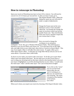
© Copyright 2026