
T-IFS-00064-2005.R1 1 that identification is possible even from processed images.
T-IFS-00064-2005.R1
1
Digital Camera Identification from Sensor
Pattern Noise
Jan Lukáš, Jessica Fridrich, and Miroslav Goljan
Abstract—In this article, we propose a new method for the
problem of digital camera identification from its images based on
the sensor’s pattern noise. For each camera under investigation,
we first determine its reference pattern noise, which serves as a
unique identification fingerprint. This is achieved by averaging
the noise obtained from multiple images using a denoising filter.
To identify the camera from a given image, we consider the
reference pattern noise as a spread spectrum watermark, whose
presence in the image is established using a correlation detector.
Experiments on approximately 320 images taken with 9
consumer digital cameras are used to estimate false alarm rates
and false rejection rates. Additionally, we study how the error
rates change with common image processing, such as JPEG
compression or gamma correction.
Index Terms—Fixed pattern noise, sensor identification, digital
forensic, pattern noise, pixel non-uniformity
I.
INTRODUCTION
As digital images and video continue to replace their analog
counterparts, the importance of reliable, inexpensive, and fast
identification of digital image origin will only increase.
Reliable identification of the device used to acquire a
particular digital image would especially prove useful in the
court for establishing the origin of images presented as
evidence. In the same manner as bullet scratches allow
forensic examiners to match a bullet to a particular barrel with
reliability high enough to be accepted in courts, a digital
equivalent of bullet scratches should allow reliable matching
of a digital image to a sensor. In this paper, we propose to use
the sensor pattern noise as the tell-tale “scratches” and show
Manuscript received December 19, 2005.
The work on this paper was supported by Air Force Research Laboratory,
Air Force Material Command, USAF, under a research grant number F3060202-2-0093. The U.S. Government is authorized to reproduce and distribute
reprints for Governmental purposes notwithstanding any copyright notation
there on. The views and conclusions contained herein are those of the authors
and should not be interpreted as necessarily representing the official policies,
either expressed or implied, of Air Force Research Laboratory, or the U.S.
Government.
Special thanks belong to Taras Holotyak for providing us with Matlab code
for the denoising filter. We would also like to thank to Paul Blythe, Antje
Schneidewind, Peter Burns, James Adams, Chris Honsinger, John Hamilton,
and George Normandin for many useful discussions.
J. Lukáš is a Ph.D. candidate at the Department of ECE, Binghamton
University, Binghamton, NY 13902 USA (607-777-5689; fax: 607-777-5689;
e-mail: [email protected]).
J. Fridrich is an Associate Professor at the Department of ECE,
Binghamton University, Binghamton, NY 13902 USA (607-777-6177; fax:
607-777-4464; e-mail: [email protected]).
M. Goljan is a Research Scientist at the Department of ECE, Binghamton
University, Binghamton, NY 13902 USA (607-777-5793; fax 607-777-4464;
e-mail: [email protected]).
that identification is possible even from processed images.
The problem of digital image authentication may be
approached from several different directions. On the most
obvious and simplest level, one could inspect the electronic
file itself and look for clues in headers or any other attached or
associated information. For instance, the EXIF header contains
information about the digital camera type and the conditions
under which the image was taken (exposure, date and time,
etc.). Additional information can be obtained from the
quantization table in the JPEG header (some cameras use
customized quantization matrices). This header data, however,
may not be available if the image is resaved in a different
format or recompressed. Another problem is the credibility of
information that can be easily replaced.
There has been some effort in the digital watermarking
community to embed in the image an invisible fragile
watermark (Epson PhotoPC 700/750Z, 800/800Z, 3000Z) or a
visible watermark (Kodak DC290), that would carry
information about the digital camera, a time stamp, or even
biometric of the person taking the image [1]. A similar
approach is used in the Canon Data Verification Kit [2] that
uses the hash of the image and a special secure memory card
to enable tracing the image to a specific Canon camera. Only
relatively expensive Canon DSLR cameras (digital singlelens-reflective) support this solution. While the idea to insert
the “bullet scratches” in the form of a watermark directly into
each image the camera takes is an elegant and empowering
solution to the image authentication and camera identification
problem, its application is limited to a closed environment,
such as “secure cameras” for taking images at crime scenes.
Under these controlled conditions, such secure cameras can,
indeed, provide a solution to the problem of evidence integrity
and origin. This approach, however, cannot solve the problem
in its entirety unless all cameras either insert watermarks or
embed secure hashes in their images.
Kharrazi et al. [4] proposed a novel idea for camera
identification based on supervised learning. In their method,
each image is represented using a vector of numerical features
extracted from it. Some features are calculated in the spatial
domain while the rest are computed in the wavelet domain as
in [5]. A multi-class SVM classifier (support vector machine)
is then trained to classify images from 5 different cameras.
The correct classification ranged from roughly 78% for the
worst case to 95% in the best case. Forensic applications at the
court are likely to require a substantially higher level of
accuracy.
Another previously investigated approach is analysis of
T-IFS-00064-2005.R1
pixel defects. In [3], the authors show that hot pixels or dead
pixels (defective pixels in general), could be used for reliable
camera identification even from lossy JPEG compressed
images. However, there are cameras that do not contain any
defective pixels or cameras that eliminate defective pixels by
post-processing their images on-board. For such cameras or
sensors, this method cannot be applied.
Kurosawa’s approach [6] is the closest in spirit to our
method but still fundamentally very different. The authors
mention the pattern noise of video-camera imaging sensors for
the purpose of camera identification. We note that the pattern
noise is defined [7] as any noise component that survives
frame averaging. However, what the authors use in their
article is just one component of this noise – the dark current
noise (also called fixed pattern noise1 [7]), which is a signal
collected from the sensor when it is not exposed to light. Dark
current can only be extracted from dark frames. This limits the
method because, as the authors themselves point out, camera
identification is not possible from regular (non-dark) frames.
The fixed pattern noise is only a small component of the
pattern noise. Another, and much stronger, component that
better survives processing, is the pixel non-uniformity noise
caused by different sensitivity of pixels to light. The method
proposed in this article primarily relies on this component.
Another important difference between our approach and [6] is
that we use correlation to establish the presence of a certain
pattern in an image, while Kurosawa at al. just amplify the
fixed pattern noise and continue detecting it as local pixel
defects.
The camera identification method based on sensor’s pattern
noise proposed in this paper gives significantly more reliable
results compared to previous approaches. Moreover, the origin
and character of some components of the pattern noise make it
a good candidate for the equivalent of biometrics for sensors
(“devicemetrics”) suitable for forensic applications.
In the next section, we describe the processing stages inside
a digital camera and explain the origin of imperfections and
noise sources. In particular, we focus on the properties of the
pattern noise. The camera identification algorithm is
introduced in Section III, where we also describe the
procedure for extracting the reference pattern for each camera
and the correlation detector. The performance of the
identification method is evaluated using false acceptance and
false rejection rates in Section IV, where we report how image
processing, such as JPEG compression or gamma correction,
influence the error rates. In Section V, we discuss other
relevant questions, such as the possibility to remove or forge
the pattern noise. The paper is concluded in Section VI.
II.
SIGNAL PROCESSING IN DIGITAL CAMERAS
In this section, we briefly describe the processing stages
inside a typical digital camera and discuss various
imperfections that inevitably enter the image acquisition
process. In particular, we focus on the pattern noise and its
1
We use the same terminology as Kurosawa et al. [6] and [7], which is,
however, different than in [8].
2
properties and evaluate which components are likely to be
useful for camera identification.
The heart of every digital camera is the imaging sensor. The
sensor is divided into very small minimal addressable picture
elements (pixels) that collect photons and convert them into
voltages that are subsequently sampled to a digital signal in an
A/D converter. Before the light from the photographed scene
reaches the sensor, however, it passes through the camera
lenses, an antialiasing (blurring) filter, and then through a
color filter array (CFA). The CFA is a mosaic of color filters
that block out a certain portion of the spectrum, allowing each
pixel to detect only one specific color. The Foveon™ X3
sensor is the only sensor that does not use CFA and is able to
capture all three basic colors at every pixel.
If the sensor uses a CFA, the digitized sensor output is
further interpolated (demosaicked) using color interpolation
algorithms to obtain all three basic colors for each pixel. The
resulting signal is then further processed using color
correction and white balance adjustment. Additional
processing includes gamma correction to adjust for the linear
response of the imaging sensor and kernel filtering to visually
enhance the image. Finally, the digital image is written to the
camera memory device in a user-selected image format. This
may require additional processing, such as JPEG compression.
A.
Imperfections and noise
There are numerous sources of imperfections and noise that
enter into various stages of the image acquisition process
above. Even if the imaging sensor takes a picture of an
absolutely evenly lit scene, the resulting digital image will still
exhibit small changes in intensity between individual pixels.
This is partly because of the shot noise (also known as
photonic noise [7], [8]), which is a random component, and
partly because of the pattern noise – a deterministic
component that stays approximately the same if multiple
pictures of the exact same scene are taken. Due to this
property, the pattern noise is present in every image the sensor
takes and thus can be used for camera identification. Because
the pattern noise is a systematic distortion, it may appear that
it is improper to call it noise. Nevertheless, by slight abuse of
language, the pattern noise is a well established term in the
imaging sensor literature [7], [8] and we accept this
terminology here as well. We note that averaging multiple
images reduces the random components and enhances the
pattern noise.
The two main components of the pattern noise are the fixed
pattern noise (FPN) and the photo-response non-uniformity
noise (PRNU) (see Fig. 1). The fixed pattern noise (FPN) is
caused by dark currents. It primarily refers to pixel-to-pixel
differences when the sensor array is not exposed to light.
Because the FPN is an additive noise, some middle to highend consumer cameras suppress this noise automatically by
subtracting a dark frame [9] from every image they take. FPN
also depends on exposure and temperature.
In natural images, the dominant part of the pattern noise is
the photo-response non-uniformity noise (PRNU). It is caused
primarily by pixel non-uniformity (PNU), which is defined as
T-IFS-00064-2005.R1
3
different sensitivity of pixels to light caused by the
inhomogenity of silicon wafers and imperfections during the
sensor manufacturing process. The character and origin of the
PNU noise make it unlikely that even sensors coming from the
same wafer would exhibit correlated PNU patterns. As such,
the PNU noise is not affected by ambient temperature or
humidity.
B.
Flat fielding
It is possible to suppress the pattern noise using a process
called flat fielding [7], [8], in which the pixel values are first
corrected for the additive FPN and then divided by a flat field
frame fˆ
ij
xˆij = ( yij − cij ) / fˆij .
(3)
In (3), xˆij is the corrected sensor output and fˆij is an
approximation to fij obtained by averaging K images of a
uniformly lit scene fij( k ) , k = 1, …, K
fˆij =
Fig. 1: Pattern noise of imaging sensors.
Light refraction on dust particles and optical surfaces and
zoom settings also contribute to the PRNU noise. These
components are known as “doughnut” patterns and vignetting
and are of low spatial frequency in nature [8]. Because these
low frequency components are not a characteristic of the
sensor, we should not use them for sensor identification and
only use the PNU component, which is an intrinsic
characteristic of the sensor.
We now describe a mathematical model of the image
acquisition process. Let us denote the photon counts that
would be ideally registered by the sensor due to incoming
light as x = (xij), i = 1, …, m, j = 1, …, n, where m×n is the
sensor resolution Denoting the shot noise as η = (ηij), the
additive random noise (represented by read-out noise, etc.) as
ε = (εij), and the dark current as c = (cij), the output of the
sensor y = (yij) can be expressed in the following form (before
any other camera processing)
pij = P(yij, N(yij), i, j),
∑
.
(4)
80
70
60
50
40
30
20
10
0
0
200
400
600
800
Frequency
1000
1200
Fig. 2: Magnitude of Fourier transform of one row in an image
obtained as average over 118 images of a flat scene.
(2)
2
where P is a non-linear function of yij, the pixel location (i, j),
and values y from a local neighborhood N(yij).
k
1
fij( k )
m × n i , j ,k
C.
Properties of pixel non-uniformity noise
In order to better understand the impact of the pattern noise
on the final image pij and to determine its properties, we
performed the following experiment. Using a light-box
producing a uniformly illuminated surface3, we took 118
images using a Canon G2 camera (for camera specifications,
see Table I below). The camera was set to automatic exposure
and was focused to infinity. The white balance was set so that
the light-box produced neutral gray images.
(1)
The factors fij are typically very close to 1 and capture the
PRNU noise, which is a multiplicative noise. As mentioned
above, the signal y goes through a long chain of complex
processing before it is stored in an image file. This processing
includes operations on a local neighborhood of pixels, such as
demosaicking, color correction, or kernel filtering. Some
operations may be non-linear in nature, such as gamma
correction, white balance, or adaptive color interpolation.
Thus, the final pixel values pij, which we will assume to be in
the range 0 ≤ pij ≤ 255, are
(k )
ij
Note that this process cannot be done correctly from the
final pixel values pij and must be performed on the raw sensor
output y before any further image processing. While it is
commonly done for astronomical imaging2, consumer digital
cameras do not flat-field their images because it is difficult to
achieve a uniform sensor illumination inside the camera.
|F|
yij = fij (xij + ηij) + cij + εij.
∑f
We note that in most scientific applications flat-fielding does not include
subtraction of the dark frame because the FPN is usually suppressed by
cooling the sensor.
3
Taking pictures of a flat scene helps reduce the impact of color
interpolation and other in-camera processing.
T-IFS-00064-2005.R1
4
All images exhibited a slight intensity gradient and
vignetting. To remove these low-frequency patterns, we
applied a high-pass filter with cut-off frequency of
(150/1136)π. After filtering, the images were averaged. The
averaging reduced the random noise components, while the
pattern noise accumulated. In Fig. 2, we show the magnitude
of the Fourier transform F(r) of one pixel row r in the
averaged image. The signal r exhibits properties of a white
noise signal with an attenuated high frequency band. This
attenuation is likely due to the low-pass character of the CFA
interpolation algorithm.
The PNU noise can not be present in completely saturated
areas of an image, where the pixels were filled to their full
capacity, producing a constant signal. It is also clear from (1)
that in very dark areas (when xij ≈ 0) the amplitude of the PNU
noise is suppressed as well, leaving the FPN as the dominant
component of the pattern noise.
We close this section with a note that essentially all imaging
sensors (CCD, CMOS, JFET, or CMOS-Foveon™ X3) are
built from semiconductors and their manufacturing techniques
are similar. Therefore, it is reasonable to expect that the
pattern noise in all these sensors has similar properties.
Although [7] and [8] deal mainly with CCDs, it is noted in [7]
(page 92) that CMOS sensors also experience both FPN and
PRNU. Moreover, according to [10] the PRNU noise strength
is comparable for both CMOS and CCD detectors. As JFET
sensors do not differ too much from CMOSs, they should also
behave similarly. Our experiments with the CMOS-Foveon™
X3 based Sigma SD9 camera confirm the presence of pattern
noise that survives frame averaging and that can be used for
camera identification.
III.
CAMERA IDENTIFICATION ALGORITHM
Because of the noise-like character of the PNU noise, it is
natural to detect its presence in an image using correlation as
is commonly done in robust watermark detection [11]. To
verify that a specific image p was taken with camera C, we
first determine the camera reference pattern PC, which is an
approximation to the PNU noise. The presence of the
reference pattern in p will be established using correlation. We
now describe this process in detail.
A.
Camera reference pattern
Because of the complex nature of the processing (2) and
because most consumer cameras do not allow access to the
raw sensor output yij, it is generally not possible to extract the
PNU noise using flat fielding. It should be, however, possible
to obtain an approximation to the PNU noise by averaging
multiple images p(k), k = 1, …, Np. This process can be sped up
by suppressing the scene content from the image prior to
averaging. This is achieved using a denoising filter F and
averaging the noise residuals n(k) instead,
n(k) = p(k) – F(p(k)).
(5)
Another benefit of working with the noise residuals is that
the low-frequency components of PRNU are automatically
suppressed. Obviously, the larger the number of images Np,
the more we suppress random noise components and the
impact of the scene. Based on our experiments, we
recommend using Np > 50.
We have experimented with several denoising filters and
eventually decided to use the wavelet-based denoising filter
described in Appendix A because it gave us the best results.
This is likely because the noise residual obtained using this
particular filter contains the least amount of traces of the scene
(areas around edges are usually misinterpreted by less
sophisticated denoising filters, such as the Wiener filter or the
median filter).
Finally, we would like to point out that there are two
advantages of this method for obtaining the reference pattern:
a) it does not require access to the camera (assuming we have
images taken by the camera), b) it is applicable to all cameras
independently of the fact whether or not the camera allows
access to raw sensor output.
B.
Detection by correlation
To decide whether a specific image p was taken by camera
C, we calculate the correlation ρC between the noise residual
n = p – F(p) and the camera reference pattern PC
ρC ( p) = corr (n, PC ) =
( n − n ) ⋅ ( PC − PC )
n − n PC − PC
,
(6)
where the bar above a symbol denotes the mean value.
We can now experimentally determine the distribution of
ρC(q) for other images q taken by C and the distribution of
ρC(q’) for images q’ that were not taken by C. Accepting a
parametric model for both distributions, we calculate a
threshold using the Neyman-Pearson approach and minimize
the false rejection rate (FRR) while imposing a bound4 on the
false acceptance rate (FAR). The value ρC(p) is then compared
to the threshold to reach the final decision.
To assess the reliability of this camera identification
algorithm, in the next section we performed several
experiments with 320 images from 9 digital cameras.
IV.
EXPERIMENTS AND RESULTS
In this section, we experimentally estimate the error rates of
the camera identification method above. We also study how
the error rates are influenced by common image processing
operations, such as JPEG compression and gamma correction.
A.
Cameras and test images
For our tests, we prepared an image database containing
approximately 320 images from each camera listed in Table I
with a variety of outdoor and indoor scenes, including closeups and landscapes taken under varying light conditions. A
few selected images are shown in Appendix B.
Images were taken with and without the flash and with
varying zoom settings. Also, these images were taken under
vastly different ambient temperatures ranging from winter
scenes taken at –10°C to scenes taken at outside temperature
4
This is because in forensic applications in general, it is important to keep
the FAR low.
T-IFS-00064-2005.R1
5
TABLE I
CAMERAS USED IN EXPERIMENTS AND THEIR PROPERTIES.
Camera brand
Sensor
Canon PowerShot A10
Canon PowerShot G2
Canon PowerShot S40
Kodak DC290
Olympus Camedia C765 UZ – 1
Olympus Camedia C765 UZ – 2
Nikon D100
Sigma SD9
Olympus Camedia C3030
1/2.7-inch CCD
1/1.8-inch CCD
1/1.8-inch CCD
unspecified CCD
1/2.5-inch CCD
1/2.5-inch CCD
23.7×15.5 mm Nikon DX CCD
20.7×13.8 mm CMOS-Foveon X3
1/1.8-inch CCD
close to 30°C and relative humidity over 90%. Images from
Olympus C3030 and Kodak DC290 were taken over a long
time span of about 5 years.
We point out that the Canon G2 and S40 share the same
CCD sensor type and the two Olympus C765 cameras are of
the exact same brand and model.
Table I shows for each camera the imaging sensor, its native
resolution, and image format in which the images (all in native
resolution if not mentioned otherwise) were taken. Images in
the Canon CRW raw format were converted using the Canon
Utilities RAW Image Converter version 1.2.1 to the 24-bit true
color TIFF format. Images taken in the Nikon NEF raw format
were converted by Nikon Capture 4.0 into the 24-bit true color
TIFF format. All images from Canon A10 and Olympus
Camedia C3030 were collected in the JPEG format. The
Sigma SD9 is a semiprofessional DSLR camera with the
CMOS-Foveon™ X3 sensor. It only outputs images in its
proprietary X3F raw format. All images were converted to 24bit TIFF using Sigma PhotoPro 2.1.
Image
format
JPEG
CRW
CRW
TIFF
TIFF
TIFF
NEF
X3F
JPEG
correlations for the correct camera and all 8 remaining
cameras are well separated, which means that we do not
observe any errors. Although substantially increasing the
number of cameras or test images is the only proper way to
estimate the errors, it is not a feasible approach in the short
term. Instead, we decided to use a conservative parametric
model of the data and obtain estimates of the error rates.
Let ρ cc ' (i ) , i = 1, …, N, denote the vector of N = 300
correlations between the reference pattern from camera c∈{1,
…, 9} with the noise residual from N images from camera c’.
Fig. 3 shows an example of the distribution of ρ cc ' (i ) for c and
c’ corresponding to Canon S40 and Olympus C765,
respectively. The shape of the distributions changes very much
for different combinations of cameras c and c’. In particular,
they may have thick tails or may be quite “spiky.” We
modeled the individual distributions of ρ cc ' (i ) , i = 1, …, N, for
fixed c and c’ using the Generalized Gaussian model with
probability density function
B.
⎛ |x−μ| ⎞
α ⎟⎠
−⎜
1
f ( x;α , β , μ ) =
e ⎝
2α Γ(1/ β )
β
.
(7)
60
50
40
Bin count
Experiment I
We calculated the reference pattern for each camera by
averaging the noise residual (5) for Np = 300 images from the
database. Then, we calculated the correlation of each reference
pattern with the noise residual from every image from the
database. Unless noted otherwise, when correlating a noise
residual with a camera reference pattern of different
dimensions, we cropped the larger of the two to fit the
dimensions of the smaller one. Because digital cameras differ
in image resolution and aspect ratios (3:2 or 4:3), cropping
seemed to be the natural choice for comparing pixel-to-pixel
differences.
For every image from the database of 9×300=2700 images,
the correlation with the reference pattern of the camera that
took the image was always the highest. The distributions were
also always well separated indicating that this method for
camera identification has good potential. To estimate the FAR
and FRR, we performed the following statistical analysis of
the experimental data.
The proper way to estimate the FAR and FRR is to collect
enough data to experience both types of errors. The
Doddington’s rule of 30 [14] requires conducting enough tests
to experience at least 30 errors. In our case, the distributions of
Native
resolution
1280×960
2272×1704
2272×1704
1792×1200
2288×1712
2288×1712
3008×2000
2268×1512
2048×1536
30
20
10
0
-0.002
-0.001
0
0.001 0.002
Correlation
0.003
0.004
Fig. 3: Distribution of correlation of the reference pattern from
Canon S40 with noise residual from 300 Olympus C765 images.
T-IFS-00064-2005.R1
6
μˆ =
1
N
N
∑ ρ (i),
i =1
βˆ = G −1 (mˆ 12 / mˆ 2 ),
Γ(1/ βˆ )
αˆ = mˆ 1
,
Γ(2 / βˆ )
(8)
where
mˆ 1 =
mˆ 2 =
G ( x) =
N
1
N
∑ ρ (i) − μˆ ,
1
N
∑ ρ (i) − μˆ
i =1
N
2
(9)
,
i =1
[Γ(2 / x)]2
,
Γ(1/ x)Γ(3 / x)
and Γ(x) is the Gamma function.
The generalized Gaussian model was used intentionally
because models that allow thicker tails will lead to more
conservative error estimates. In Fig. 4, we show an example of
the distribution of correlations between the reference pattern
from Olympus C3030 and noise residual from Canon G2 and
the corresponding generalized Gaussian model fit.
the distributions of ρ cc ' (i ) for individual pairs of c and c’ are
well modeled using the generalized Gaussian, when pooled
together, they no longer follow the model. Therefore, we
carried out the error analysis in the following manner.
Let Fcc ' , 1 ≤ c, c’ ≤ 9, be the cumulative density function of
the generalized Gaussian distribution (7) with parameters
(α , β , μ ) determined from correlations ρ cc ' (i ) , i = 1, …, Np,
between the reference pattern of the c-th camera and the noise
residual of N = 300 images taken by camera c’. To decide
whether camera c0 took a given image p, we calculate the
correlation ρ between the noise residual of p and the reference
pattern of camera c0 and compare to a threshold t for this
camera. If ρ > t, we will conclude that p was taken with
camera c0. In forensic applications, it is important to minimize
the probability of false acceptance. Thus, we use the NeymanPearson approach and determine the value of t by maximizing
the probability of detection (or, equivalently minimizing the
FRR) given an upper bound on the FAR, FAR < αFAR.
350
300
250
Bin count
The parameters were estimated using the method of
moments [15]. In particular, given a vector of correlations
ρ(i), i = 1, …, N,
200
150
450
100
400
350
50
300
0
-0.02 -0.015 -0.01 -0.005 0 0.005 0.01 0.015 0.02
Correlation
250
200
Fig. 5: Distribution of correlation of the reference pattern from Nikon
D100 with noise residual from approx. 8×300 images from all other
cameras.
150
100
For a given threshold t, the probability of false rejection is
50
0
-0.015 -0.01 -0.005
0
0.005
Correlation
0.01
0.015
0.02
Fig. 4: Distribution of correlation (plus signs) and its generalized
Gaussian fit (line) with the shape parameter β = 1.173.
We could estimate the FAR and the FRR for each camera c
by fitting the model to the distribution of ρ cc (i ) , i = 1, …, N,
and modeling
ρ cc ' (i )
FRR = Fcc0 (t ) .
Assuming p was not taken by camera c0 but is classified as
coming from c0 based on threshold t, we obtain
9
FAR = 1 −
∏F
c =1
c ≠ c0
, i = 1, …, N, for all cameras c’≠ c as one
signal. However, when pooling the correlations ρ cc ' (i ) for all
cameras c ≠ c’, the resulting distribution may be multi-modal
(see Fig. 5). This is because the reference patterns of some
cameras exhibit a small positive correlation (e.g., Canon S40,
Canon G2, and Nikon D100). We hypothesize that this small
correlation is due to similar in-camera processing, such as the
same CFA interpolation algorithm. Consequently, although
(10)
0
c
c0 (t )
.
(11)
Thus, the FRR will be minimized for the largest t that satisfies
9
1−
∏F
c =1
c ≠ c0
c
c0 (t )
≤ α FAR .
(12)
T-IFS-00064-2005.R1
7
TABLE II
DECISION THRESHOLD
Processing
Camera
Nikon
C765 - 1
C765 - 2
G2
S40
Sigma
Kodak
C3030
A10
Processing
Camera
Nikon
C765 - 1
C765 - 2
G2
S40
Sigma
Kodak
t
AND FRR FOR ALL 9 DIGITAL CAMERAS FOR FAR
none
t
FRR
0.0449
4.68×10⁻³
0.0170
3.79×10⁻⁴
0.0080 5.75×10⁻¹¹
0.0297
2.31×10⁻⁴
0.0322
1.42×10⁻⁴
0.0063
2.73×10⁻⁴
0.0097 1.14×10⁻¹¹
0.0209
1.87×10⁻³
0.0166
7.59×10⁻⁵
JPEG 90
t
FRR
0.0225
3.71×10⁻³
0.0122
5.36×10⁻⁶
0.0061
0
0.0097 8.99×10⁻¹¹
0.0133 3.96×10⁻¹¹
0.0050
3.44×10⁻⁶
0.0107
2.27×10⁻⁹
Gamma 0.7
t
FRR
0.0443
1.09×10⁻²
0.0163
3.88×10⁻⁴
0.0076
2.57×10⁻¹¹
0.0271
3.23×10⁻⁴
0.0298
1.64×10⁻⁴
0.0060
2.93×10⁻⁴
0.0096
1.08×10⁻⁸
0.0216
1.58×10⁻³
0.0162
4.71×10⁻⁵
JPEG 70
t
FRR
0.0231
5.83×10⁻²
0.0064
1.55×10⁻⁶
0.0065
9.63×10⁻¹⁴
0.0079
4.85×10⁻¹¹
0.0085
4.41×10⁻¹⁴
0.0055
9.16×10⁻⁶
0.0127
4.53×10⁻⁴
Because (11) is monotonically decreasing with t, we find the
threshold t by solving (12) where we replace the inequality
sign with equality. In each particular case, this equation must
be solved numerically. Once the threshold is found, the FRR is
determined from (10).
The first two columns in Table II show the FRR for all 9
cameras when the decision threshold was set to obtain FAR =
10–3. We point out that it is possible to distinguish between the
two Olympus C765 cameras of the exact same brand and
model. This supports our choice of the PNU noise as
“biometrics” for sensors.
The identification is successful for Canon A10 and
Olympus C3030, although their images were only available as
JPEGs and their reference patterns were also calculated from
JPEG images rather than uncompressed TIFF images.
Also note in Table II that reliable camera identification is
possible for the Sigma SD9 camera equipped with a CMOS
sensor.
Table II indicates that the camera identification is the least
reliable for Nikon D100. This is because the distribution of
correlations between the Nikon reference pattern with noise
residuals from other cameras has thicker tails than for other
cameras (e.g., the shape parameter β = 0.78 for images from
Canon A10). This increases the FRR. We hypothesize that the
reason for this is the physical size of pixels. Semi-professional
DSLR sensors have larger physical dimensions than those in
compact digital cameras and thus larger pixels. Therefore, the
PNU noise will be less pronounced due to averaging material
inhomogenities over a larger area and more robust
manufacturing, while random noise components are more
likely to increase.
C.
Experiment II (gamma correction)
Digital images are often subjected to point-wise operations,
such as brightness/contrast adjustment or gamma correction.
= 10−3.
Gamma 1.4
t
FRR
0.0435 6.33×10⁻³
0.0172 3.85×10⁻⁴
0.0081 2.83×10⁻¹⁰
0.0313 4.78×10⁻⁵
0.0343 1.02×10⁻⁴
0.0064 2.76×10⁻⁴
0.0094 3.73×10⁻¹³
0.0195 2.67×10⁻³
0.0160 2.93×10⁻⁴
JPEG 50
t
FRR
0.0210 1.63×10⁻¹
0.0060 1.17×10⁻⁴
0.0065 2.14×10⁻⁶
0.0076 5.13×10⁻⁴
0.0083 9.48×10⁻⁵
0.0059 6.57×10⁻⁵
0.0131 4.65×10⁻³
Because most spread spectrum watermarks [11] are fairly
insensitive to such operations, the camera identification
procedure is expected to be fairly robust to gamma
adjustment, as well.
We repeated Experiment I after processing images from all
cameras using gamma correction with γ = 0.7 and 1.4. These
two values were chosen as the minimal and maximal gamma
values that one can typically encounter in practice. JPEG
images from Canon A10 and Olympus C3030 cameras were
converted to bitmaps first and then gamma corrected.
The results in terms of FRR are shown in Table II in
corresponding columns. The results confirm our expectations
that gamma correction has little influence on the reliability of
camera identification.
D.
Experiment III (JPEG compression)
Because it is likely that in practice images will be stored in
the lossy JPEG format, in this section we investigate the
impact of JPEG compression on the reliability of camera
identification.
In Experiment I, all images from Canon A10 and Olympus
C3030 were already taken in the JPEG format (JPEG quality
factor approximately 93–97 for Canon A10 and 70–95 for
Olympus C3030). This indicates that the identification method
is robust to JPEG compression. We decided to verify this
claim for the remaining 7 cameras under more controlled
conditions. We repeated Experiment I after saving all 7×300
images as JPEGs with quality factors 50, 70, and 90.5
In Table II, we show the FRR for a fixed FAR = 10–3 for
JPEG quality factors 90, 70, and 50. For quality factor 90, we
can see that, with the exception of Kodak DC290, the FRRs
decreased when compared to the results obtained for raw
5
Reference patterns were obtained from raw images as before.
T-IFS-00064-2005.R1
8
images (the first two columns in Table II). We now attempt to
explain this somewhat surprising result.
Although JPEG compression does decrease the average
value of correlations between the image noise residual and the
correct reference pattern, it does so very gradually with the
decreasing quality factor. However, we observed that JPEG
compression with quality factor 90 or less almost completely
suppresses the small positive correlations between the
reference patterns that can be seen in Fig. 5 (compare with
Fig. 6). Additionally, JPEG compression makes the tails of the
distributions ρ cc ' (i ) , for c ≠ c’ somewhat thinner. The
combined effect of both phenomena results in more reliable
identification.
250
Sigma SD9, and Kodak DC290). For the remaining 6 cameras,
we simply resampled6 each noise residual to the native
resolution of each camera and then computed the correlation
with its reference pattern.
Due to the small number of images, we did not analyze the
results statistically as in the previous sections. Instead, we
only include in Fig. 7 a scatter plot of correlation values
between the noise residual from all 84 images with all 6
reference patterns. We see that the correlation with Canon G2
camera was always the highest even for the low-quality JPEGs
(images 6–33).
We note that a much more extensive experiment performed
on more images and across all cameras is necessary to
determine the error rates of camera identification from lowresolution images. This preliminary result is, nevertheless,
encouraging.
200
0.12
150
Correlation
Bin count
G2
0.1
100
50
S40
0.08
A10
C765 - 1
0.06
C765 - 2
C3030
0.04
0.02
0
-0.015
-0.01
-0.005
0
0.005
Correlation
0.01
0.015
0
-0.02
Fig. 6: Distribution of correlation of the reference pattern from Nikon
D100 with noise residual from approximately 6×300 JPEG
compressed images with quality factor 90 from six other cameras.
E.
Experiment IV (resampling and JPEG compression)
Most digital cameras have an option to save images at lower
resolutions than the maximal resolution supported by their
sensor. In this section, we report some preliminary results of
our investigation whether or not it is possible to identify
images already taken at a lower resolution. We note that it is
not possible to simulate the resizing off line on a computer
without a detailed knowledge of how each camera produces
images of smaller resolution. Because this information is
considered proprietary by most camera manufacturers, we had
to prepare a new test database of images already taken at
lower resolution. For this reason, we limited this investigation
to just one camera – Canon G2.
We set the camera to take images at a lower resolution of
1600×1200 and took 84 test images. Total of 28 images were
taken at low-quality setting (average JPEG quality factor of
72), while the remaining 56 images were taken at the highestquality setting (with average quality factor 97). We now wish
to decide which of the 9 cameras in our tests most likely took
the images.
Let us assume for simplicity that we know that the images
were taken at a lower resolution or were rescaled on a
computer, but have not been cropped. This assumption rules
out cameras with the 3:2 image aspect ratio (Nikon D100,
0
20
40
Pictures
60
80
Fig. 7: Correlation of noise residuals from 84 Canon G2 1600×1200
JPEG images with 6 reference patterns.
F.
Experiment V (stability of pattern noise over time)
If the pattern noise is to be used for forensic camera
identification, it must be stable over a wide range of
environmental conditions, camera settings (zoom, ISO, etc.),
and over time. Since our image databases contained images
taken under widely varying environmental conditions,
different zoom and ISO settings, and battery status, the results
of Section IV indicate that the pattern noise is fairly stable.
However, all test images were taken over a relatively short
period of time of 1–2 years. The stability of the camera
identification algorithm over time is the subject of this section.
TABLE III
AVERAGE CORRELATION OVER TIME.
Year
Correlation
2000
0.055
2001
0.044
2002
0.056
2003
0.047
2004
0.047
2005
0.053
We narrowed this experiment to the Kodak DC 290 camera
because this was the only camera for which we had images
taken over a span of many years (2000–2005). All images
were taken at full resolution 1200×1792 in the JPEG format
6
Bicubic resampling was used in all experiments.
T-IFS-00064-2005.R1
("better quality" as defined in camera specifications). The
number of images ranged from 56 for year 2001 to more than
700 for year 2003. For each year, we computed the average
correlation with the reference pattern obtained from pictures
taken in the first quarter of 2004. Table III indicates that the
average correlation value varies very little over time.
V.
FORGING AND MALICIOUS PROCESSING
Since camera identification techniques are likely to be used
in the court, we need to address malicious attacks intended to
fool the identification algorithm, such as intentionally
removing the pattern noise from an image to prevent
identification or extracting the noise and copying it to another
image to make it appear as if the image was taken with a
particular camera.
We distinguish two situations: 1) the attacker is informed
and has either the camera or many images taken by the camera
or 2) the attacker is uninformed in the sense that he only has
access to one image.
We first discuss the issue of removing the pattern noise or
preventing its successful detection. As already noted in
Section II.B, an informed attacker can suppress the pattern
noise by dark frame subtraction and flat-fielding. However,
images are not typically stored in raw formats and are only
available as TIFF/JPEG, which means they are already
processed in the camera (Eq. (2) in Section II). As a result, it
is in general not possible to perform flat fielding correctly
from a TIFF/JPEG image.
A simpler way to remove the pattern noise PC, well-known
to researchers working in robust watermarking, is as follows.
The attacker can arrange for ρC = 0 for any image p taken with
C by solving the equation corr(p+αPC, PC) = 0 with respect to
α and taking p+αPC as the forged image.
An uninformed attacker could attempt to remove the pattern
noise by applying the same denoising filter. While this,
indeed, decreases the correlation value with the correct pattern
approximately by a factor of two, in most cases correct
identification will still be possible. However, repetitive
application of the filter or more aggressive denoising filters
will likely prevent correct identification.
The easiest way to prevent a simple detection of the
reference pattern is desynchronization, such as slight rotation,
possibly combined with other processing that might include
resizing, cropping, and filtering. Probably the simplest active
measure that the photographer can use to complicate image
identification later is to take images using a continuous digital
zoom, a feature that many consumer digital cameras have
today.
The second problem we now investigate is whether it is
possible to make an arbitrary image look as if it was taken by
a specific camera. Again, having access to the reference
pattern or the camera makes this indeed possible. We denoised
20 Canon G2 pictures and added to them the reference pattern
from Canon S40. We increased the amplitude of the added
noise, till we reached a correlation that was higher than the
correlation the image previously had with the Canon G2
9
reference pattern. The peak signal to noise ratio (PSNR) for
the forged images was on average 37.5dB and the images were
visually indistinguishable from originals. The forgeries still
had higher correlations with the Canon G2 reference pattern
than expected from different camera images, but this
correlation could be eliminated using some of the techniques
mentioned above.
We also tried to plant the noise extracted from a single
Canon S40 image using the denoising filter [12] into a
denoised Canon G2 image. The correlation of the noise
extracted from the resulting image with the Canon S40
reference pattern was usually within the range of the typical
correlation values achieved by other Canon S40 images. This
kind of malicious processing requires multiplying the added
noise with a perceptual mask [11] to avoid creating visible
artifacts.
Overall, we conclude that malicious manipulation that will
fool the identification algorithm is, indeed, possible if the
attacker possesses enough skill in signal processing. We note
that it is unlikely that there exists a numerical identification
characteristic computed from digital images that could not be
compromised by a sufficiently sophisticated opponent. All
previously proposed techniques based on defective pixels [3]
[6] or image features [4], are certainly vulnerable to malicious
attacks as well.
VI.
CONCLUSIONS
We have developed a new approach to the problem of
camera identification from images. Our identification method
uses the pixel non-uniformity noise which is a stochastic
component of the pattern noise common to all digital imaging
sensors (CCD, CMOS, including Foveon™ X3, and JFET).
The presence of this noise is established using correlation as in
detection of spread spectrum watermarks. We investigated the
reliability of camera identification from images processed
using JPEG compression, gamma correction, and a
combination of JPEG compression and in-camera resampling.
Experimental results were evaluated using FAR and FRR error
rates. We note that the proposed method was successful in
distinguishing between two cameras of the same brand and
model.
Since the identification technique requires proper
synchronization, geometrical operations, such as cropping,
resizing, rotation, digital zoom, cause desynchronization and
prevent correct camera identification. In this case, the
detection algorithm will have to resort to brute force searches.
Techniques, such as the one described in [16], may help us
alleviate the computational complexity of brute force searches
by retrieving some information about applied geometrical
operations. The searches will, however, inevitably increase the
FAR.
We would like to point out that the problem of camera
identification should be approached from multiple directions,
combining the evidence from other methods, such as the
feature-based identification [4], which is less likely to be
influenced by geometrical transformations.
Our future plans include developing methods for detection
T-IFS-00064-2005.R1
10
of digital forgeries by detecting the presence of the pattern
noise in disjoint regions. Finally, we plan to extend this
technique to identification of video-cameras and scanners.
REFERENCES
[1]
[2]
[3]
[4]
[5]
[6]
[7]
[8]
[9]
[10]
[11]
[12]
[13]
[14]
[15]
[16]
Blythe, P. and Fridrich, J.: “Secure Digital Camera,” Digital Forensic
Research Workshop, Baltimore, August 11–13, 2004.
“Canon Data Verification Kit DVK-E2,” available:
http://www.dpreview.com/news/0401/04012903canondvke2.asp .
Geradts, Z., Bijhold, J., Kieft, M., Kurosawa, K., Kuroki, K., and Saitoh,
N.: “Methods for Identification of Images Acquired with Digital
Cameras,” Proc. of SPIE, Enabling Technologies for Law Enforcement
and Security, vol. 4232, pp. 505–512, February 2001.
Kharrazi, M., Sencar, H. T., and Memon, N.: “Blind Source Camera
Identification,” Proc. ICIP’ 04, Singapore, October 24–27, 2004.
Farid, H. and Lyu, S.: “Detecting Hidden Messages Using Higher-Order
Statistics and Support Vector Machines,” in F.A.P. Petitcolas (ed.): 5th
International Workshop on Information Hiding, LNCS vol. 2578,
Springer-Verlag, Berlin-Heidelberg, New York, pp. 340–354, 2002.
Kurosawa, K., Kuroki, K., and Saitoh, N.: “CCD Fingerprint Method Identification of a Video Camera from Videotaped Images,” Proc of
ICIP' 99, Kobe, Japan, pp. 537–540, October 1999.
Holst, G. C.: CCD Arrays, Cameras, and Displays, 2nd edition, JCD
Publishing & SPIE Pres, USA, 1998.
Janesick, J. R.: Scientific Charge-Coupled Devices, SPIE PRESS
Monograph vol. PM83, SPIE–The International Society for Optical
Engineering, January, 2001.
“Dark Frame Subtraction,” Qimage help, available:
http://www.ddisoftware.com/qimage/qimagehlp/dark.htm.
Janesick, J. R.: "Dueling Detectors", OE Magazine, vol. 2(2), February
2002.
Cox, I., Miller, M.L., and Bloom, J.A.: Digital Watermarking, Morgan
Kaufmann, San Francisco, 2001.
Mihcak M.K., Kozintsev, I., and Ramchandran, K.: “Spatially adaptive
statistical modeling of wavelet image coefficients and its application to
denoising,” in Proc. IEEE Int. Conf. Acoustics, Speech, and Signal
Processing, Phoenix, AZ, Mar. 1999, vol. 6, pp. 3253–3256.
Donoho, D., Duncan, M. R., Huo, X., and Levi, O.: Wavelab 802,
available: http://www-stat.stanford.edu/~wavelab/ .
Doddington, G., Liggett, W., Martin, A., Przybocki, M., and Reynolds,
D.: “Sheep, Goats, Lambs and Wolves: A Statistical Analysis of Speaker
Performance in the NIST 1998 Speaker Recognition Evaluation,” in
Proceedings of 5th International Conference of Spoken Language
Processing, ICSLP 98, Sydney, Australia. Paper 608 on CD-ROM.
Meignen, S. and Meignen, H.: “On the Modeling of DCT and Subband
Image Data for Compression,” IEEE Trans. on Image Processing, vol. 4,
pp. 186–193, 1995.
Popescu, A.C. and Farid H.: “Statistical Tools for Digital Forensic,” in J.
Fridrich (ed.): 6th International Workshop on Information Hiding, LNCS
vol. 3200, Springer-Verlag, Berlin-Heidelberg, New York, pp. 128–147,
2004.
APPENDIX A (DENOISING FILTER)
Our implementation of the denoising filter is based on the
work proposed in [12]. It is constructed in the wavelet domain
using the Wavelab package [13]. Let us assume that the image
is a grayscale 512×512 image. Larger images can be processed
by blocks and color images are denoised for each color
channel separately. The high-frequency wavelet coefficients of
the noisy image are modeled as an additive mixture of a
locally stationary i.i.d. signal with zero mean (the noise-free
image) and a stationary white Gaussian noise N (0, σ 02 ) (the
noise component). The denoising filter is built in two stages.
In the first stage, we estimate the local image variance, while
in the second stage the local Wiener filter is used to obtain an
estimate of the denoised image in the wavelet domain. We
now describe the individual steps:
Step 1. Calculate the fourth-level wavelet decomposition of
the noisy image with the 8-tap Daubechies QMF. We describe
the procedure for one fixed level (it is executed for the highfrequency bands for all four levels). Denote the vertical,
horizontal, and diagonal subbands as h(i, j), v(i, j), d(i, j),
where (i, j) runs through an index set J that depends on the
decomposition level.
Step 2. In each subband, estimate the local variance of the
original noise-free image for each wavelet coefficient using
the MAP estimation for 4 sizes of a square W×W
neighborhood N, for W∈{3, 5, 7, 9}.
⎛
1
2
⎝ W
σˆW2 (i, j ) = max ⎜ 0,
⎞
h 2 (i, j ) −σ 02 ⎟ , (i, j)∈J.
( i , j )∈N
⎠
∑
Take the minimum of the 4 variances as the final estimate,
σˆ 2 (i, j ) = min (σ 32 (i, j ), σ 52 (i, j ), σ 72 (i, j ), σ 92 (i, j ) ) , (i, j)∈J.
Step 3. The denoised wavelet coefficients are obtained using
the Wiener filter
hden (i, j ) = h(i, j )
σˆ 2 (i, j )
σˆ 2 (i, j ) + σ 0 2
and similarly for v(i, j), and d(i, j), (i, j)∈J.
Step 4. Repeat Steps 1–3 for each level and each color
channel. The denoised image is obtained by applying the
inverse wavelet transform to the denoised wavelet
coefficients.
To complete the description of the denoising filter, we now
briefly discuss the choice of the parameter σ0 by investigating
how the correlations between noise residuals and reference
patterns are influenced when setting σ0 to different values. We
used the reference pattern for the Canon G2 camera obtained
in Section II.C by averaging 118 uniform gray images. Note
that we do not need the filter for this. Using the filter with
parameter σ0∈{1, …, 6}, we calculated the noise residual for
20 images from each camera (20×9=180 images total). Then,
we computed the correlations between the G2 reference
pattern above and the noise residual from all 180 images. Fig.
8 shows the correlations averaged over all 20 images for each
camera as a function of σ0. This figure shows that the
dependence of the correlations on σ0 is relatively flat (the
small positive bias between G2 and S40 is commented upon in
Section II.B.).
In all experiments, we used σ0 = 5 (for dynamic range of
images 0, …, 255) to be conservative and to make sure that
the filter extracts substantial part of the PNU noise even for
cameras with a large noise component.
T-IFS-00064-2005.R1
11
Average correlation
0.15
G2
S40
A10
C765 -1
C765 - 2
C3030
Nikon
Sigma
Kodak
0.1
0.05
0
1
2
3
4
5
6
σ
Fig. 8: Correlation between the G2 reference pattern and the noise
component from images from other cameras obtained using the
denoising filter with parameter σ.
APPENDIX B
A few sample images used in our experiments:
Jan Lukáš has received his MS in Applied
Mathematics from Czech Technical University in
Prague in 1998.
He is a Ph.D. Candidate at the Dept. of Electrical and
Computer Engineering at Binghamton University
(SUNY). His main reasearch interests are in Digital
Image Forensic, Digital Image Authentication and
Digital Forgeries Detection.
Mr. Lukáš's research work has been already
appreciated by Best Student Paper Award at Image
& Video Communications and Processing 2005 (part of SPIE Electronic
Imaging 2005) and by Graduate Student Excellence in Research Award at
Binghamton University in spring 2006.
Jessica Fridrich holds the position of Associate
Professor at the Dept. of Electrical and Computer
Engineering at Binghamton University (SUNY).
She has received her PhD in Systems Science from
Binghamton University in 1995 and MS in Applied
Mathematics from Czech Technical University in
Prague in 1987. Her main interests are in
Steganography, Steganalysis, Digital Watermarking,
and Digital Image Forensic.
Dr. Fridrich's research work has been generously
supported by the US Air Force. Since 1995, she received 18 research grants
totaling over $5mil for projects on data embedding and steganalysis that lead
to more than 80 papers and 7 US patents. Dr. Fridrich is a member of IEEE
and ACM.
Miroslav Goljan received the M.S. degree in
mathematical informatics from Charles University in
Prague, Czech Republic, in 1984 and the Ph.D. in
electrical engineering from Binghamton University,
State University of New York, in 2002.
He is a Research Scientist at the Department of
Electrical and Computer Engineering, Binghamton
University. His research focuses on steganography,
steganalysis,
reversible
data
hiding
and
watermarking, and digital media authentication.

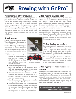


© Copyright 2026