
Document 1 - DROPS - Series
Report from Dagstuhl Seminar 14481
Multiscale Spatial Computational Systems Biology
Edited by
David Gilbert1 , Monika Heiner2 , Koichi Takahashi3 , and
Adelinde M. Uhrmacher4
1
2
3
4
Brunel University, GB, [email protected]
BTU Cottbus, DE, [email protected]
Osaka University, JP, [email protected]
Universität Rostock, DE, [email protected]
Abstract
This report documents the program and the outcomes of Dagstuhl Seminar 14481 “Multiscale
Spatial Computational Systems Biology”. This seminar explored challenges arising from the need
to model and analyse complex biological systems at multiple scales (spatial and temporal), which
falls within the general remit of Computational Systems Biology. A distinguishing factor of the
seminar was the modelling exercise – where teams explored different modelling paradigms, in
order to better understand the details of the approaches, their challenges, potential applications,
and their pros and cons. This activity was carried out in a collaborative and self-directed manner
using the Open Space Technology approach as evidenced by a high degree of communication
both within and between the teams. Eight teams were formed, and reports from five of them are
included in this document.
Seminar November 24–28, 2014 – http://www.dagstuhl.de/14481
1998 ACM Subject Classification D.2.1 Requirements/Specifications, D.2.2 Design Tools and
Techniques, D.2.4 Software/Program Verification, J.3 Biology and genetics
Keywords and phrases Multiscale, multidimensional, computational modelling, space, time, systems biology, synthetic biology
Digital Object Identifier 10.4230/DagRep.4.11.138
1
Executive Summary
David Gilbert
Monika Heiner
Koichi Takahashi
Adelinde M. Uhrmacher
License
Creative Commons BY 3.0 Unported license
© David Gilbert, Monika Heiner, Koichi Takahashi, and Adelinde M. Uhrmacher
This seminar built on the tradition of two previous Dagstuhl seminars on Formal Methods
in Molecular Biology in 2009 and 2011 (Seminar 09091, Seminar 11151), but with a special
focus on multiscale and spatial modeling and simulation.
Multiscale modelling goes beyond the traditional approach of modelling at just one
spatial/temporal scale or organizational level. Until now most models have largely ignored
locality within the cell, or cell-cell interactions. However, with the insight that spatial
phenomena like localisation and crowding have a considerable influence on reaction processes
and many processes cannot be understood with reference to one organisation level only (intraExcept where otherwise noted, content of this report is licensed
under a Creative Commons BY 3.0 Unported license
Multiscale Spatial Computational Systems Biology, Dagstuhl Reports, Vol. 4, Issue 11, pp. 138–226
Editors: David Gilbert, Monika Heiner, Koichi Takahashi, and Adelinde M. Uhrmacher
Dagstuhl Reports
Schloss Dagstuhl – Leibniz-Zentrum für Informatik, Dagstuhl Publishing, Germany
David Gilbert, Monika Heiner, Koichi Takahashi, and Adelinde M. Uhrmacher
139
or inter-cellular dynamics), the need for effective and efficient modelling and simulation
approaches arises.
The challenges for computer science and mathematics include the development of suitable
modelling approaches and associated tools to create coherent descriptions of biological systems
by integrating several spatial and/or temporal scales, and methods for the simulation and
analysis of the models.
The overall motivation for this seminar was the exploration of the most recent advances
in these methods. The seminar brought together researchers working in modelling and
analysis of biological systems with diverse professional backgrounds, including informaticians,
mathematicians, engineers, biologists, physicians.
A distinguishing factor of the seminar was the modelling exercise – where teams explored
different modelling paradigms, in order to better understand the details of the approaches,
their challenges, potential applications, and their pros and cons. This activity was carried
out in a collaborative and self-directed manner using the Open Space Technology approach
as evidenced by a high degree of communication both within and between the teams. Eight
teams were formed, and reports from five of them are included in this document (see Section 4).
The teams were formed around the following focii:
Small GTP-ase pathway.
Continuous multiscale models for biological tissue.
Simulating macromolecular crowding with particle and lattice-based methods
Multiscale modeling of S1P metabolism, secretion and signaling
DNA structural dynamics.
Dictyostelium discoideum: Aggregation and Synchronisation of Amoebas in Time and
Space.
Towards a standard exchange format for spatial, multilevel multicellular models.
Model checking for multiscale spatial biological systems.
The participants decided to take forward the activities in the future outside Dagstuhl,
with the goals of carrying out collaborative research, producing scientific papers and applying
for larger scale funded international research projects.
14481
140
14481 – Multiscale Spatial Computational Systems Biology
2
Table of Contents
Executive Summary
David Gilbert, Monika Heiner, Koichi Takahashi, and Adelinde M. Uhrmacher . . 138
Overview of Talks
The Smoldyn simulator: overview, applications, and hybrid simulation
Steven Andrews . . . . . . . . . . . . . . . . . . . . . . . . . . . . . . . . . . . . . . 143
Some cell biology modeling projects
Steven Andrews . . . . . . . . . . . . . . . . . . . . . . . . . . . . . . . . . . . . . . 143
Spatiocyte: a stochastic particle simulator for filament, membrane and cytosolic
reaction-diffusion processes
Satya Arjunan . . . . . . . . . . . . . . . . . . . . . . . . . . . . . . . . . . . . . . 143
Approximate analysis of biological systems by hybrid switching jump diffusion
Marco Beccuti . . . . . . . . . . . . . . . . . . . . . . . . . . . . . . . . . . . . . . . 144
Reaction-diffusion & particle-based simulation, and a rule-based language
Arne Bittig . . . . . . . . . . . . . . . . . . . . . . . . . . . . . . . . . . . . . . . . 145
A Modular Framework for Biomodel Engineering
Mary Ann Blätke . . . . . . . . . . . . . . . . . . . . . . . . . . . . . . . . . . . . . 145
Logic based analysis of spatio-temporal behaviour
Luca Bortolussi . . . . . . . . . . . . . . . . . . . . . . . . . . . . . . . . . . . . . . 146
Bifurcation analysis of multiscale spatial models
Lutz Brusch . . . . . . . . . . . . . . . . . . . . . . . . . . . . . . . . . . . . . . . . 147
Modulation of biological function by structure and inter-subject variability
Alfonso Bueno-Orovio . . . . . . . . . . . . . . . . . . . . . . . . . . . . . . . . . . 148
Integrative strategy to elucidate the multiple layers of the transcriptional regulation
Francesca Cordero . . . . . . . . . . . . . . . . . . . . . . . . . . . . . . . . . . . . 149
Cellular automaton models for collective cell behaviour
Andreas Deutsch . . . . . . . . . . . . . . . . . . . . . . . . . . . . . . . . . . . . . 149
Stochastic and Multiscale Modelling in Molecular, Cell and Population Biology
Radek Erban . . . . . . . . . . . . . . . . . . . . . . . . . . . . . . . . . . . . . . . 150
Mesoscopic Simulation and Visualization in Systems Biology
Martin Falk . . . . . . . . . . . . . . . . . . . . . . . . . . . . . . . . . . . . . . . . 151
Modeling the cancer stem cell theory and tumor heterogeneity
Chiara Fornari . . . . . . . . . . . . . . . . . . . . . . . . . . . . . . . . . . . . . . 151
Computational Platform for Systems Biology
Akira Funahashi . . . . . . . . . . . . . . . . . . . . . . . . . . . . . . . . . . . . . 152
Multicsale modeling of sphingolipids metabolism
Anna Gambin . . . . . . . . . . . . . . . . . . . . . . . . . . . . . . . . . . . . . . . 153
A Modular Framework for Biomodel Engineering
David Gilbert . . . . . . . . . . . . . . . . . . . . . . . . . . . . . . . . . . . . . . . 154
Quantitative modeling for Systems Biology.
Simon Hardy . . . . . . . . . . . . . . . . . . . . . . . . . . . . . . . . . . . . . . . 155
David Gilbert, Monika Heiner, Koichi Takahashi, and Adelinde M. Uhrmacher
141
From Petri Nets to PDEs in 3 Minutes
Monika Heiner . . . . . . . . . . . . . . . . . . . . . . . . . . . . . . . . . . . . . . 155
Computational Steering of Multiscale Models
Mostafa Herajy . . . . . . . . . . . . . . . . . . . . . . . . . . . . . . . . . . . . . . 157
From Networks to Function – Computational Models of Organogenesis
Dagmar Iber . . . . . . . . . . . . . . . . . . . . . . . . . . . . . . . . . . . . . . . . 158
E-Cell system version 4: Development of an integrated platform for particle simulations
Kazunari Kaizu . . . . . . . . . . . . . . . . . . . . . . . . . . . . . . . . . . . . . . 158
Information in Biological Reaction Netwroks
Tetsuya J. Kobayashi . . . . . . . . . . . . . . . . . . . . . . . . . . . . . . . . . . . 159
Spatial stochastic reaction kinetics of bistable systems: A challenge for multiscale
modeling
Marek Kochanczyk . . . . . . . . . . . . . . . . . . . . . . . . . . . . . . . . . . . . 160
Colored Petri Nets for Multiscale Systems Biology
Fei Liu . . . . . . . . . . . . . . . . . . . . . . . . . . . . . . . . . . . . . . . . . . . 160
Equivalence and simplification of reaction networks
Guillaume Madelaine . . . . . . . . . . . . . . . . . . . . . . . . . . . . . . . . . . . 161
Cancer systems biology at multiple levels
Carsten Maus . . . . . . . . . . . . . . . . . . . . . . . . . . . . . . . . . . . . . . . 162
Formal validation of multidimensional computational models
Ovidiu Pârvu . . . . . . . . . . . . . . . . . . . . . . . . . . . . . . . . . . . . . . . 163
A unifying Petri net framework for multi-scale modelling
Christian Rohr . . . . . . . . . . . . . . . . . . . . . . . . . . . . . . . . . . . . . . 163
Bayesian methodologies in statistical systems biology
Guido Sanguinetti . . . . . . . . . . . . . . . . . . . . . . . . . . . . . . . . . . . . . 164
Cell simulation – towards in silico prediction of phenotype from genotype
Koichi Takahashi . . . . . . . . . . . . . . . . . . . . . . . . . . . . . . . . . . . . . 165
Spying “Minorities” in the Cell
Yuichi Togashi . . . . . . . . . . . . . . . . . . . . . . . . . . . . . . . . . . . . . . . 165
Work on spatial modeling and simulation in cell biology at the modeling and
simulation group in Rostock
Adelinde M. Uhrmacher . . . . . . . . . . . . . . . . . . . . . . . . . . . . . . . . . 166
A short introduction into rule-based spatial multi-level modeling and simulation
Adelinde M. Uhrmacher . . . . . . . . . . . . . . . . . . . . . . . . . . . . . . . . . 168
Working Groups
Simulating macromolecular crowding with particle and lattice-based methods
(Team 3)
Steven S. Andrews, Satya N. V. Arjunan, Gianfranco Balbo, Arne T. Bittig, Jerome
Feret, Kazunari Kaizu, and Fei Liu . . . . . . . . . . . . . . . . . . . . . . . . . . . 170
14481
142
14481 – Multiscale Spatial Computational Systems Biology
Multiscale modeling of S1P metabolism, secretion and signaling (Team 4)
Francesca Cordero, Anna Gambin, Andrzej Kierzek, Guillaume Madelaine, Joachim
Niehren, Christian Rohr, and Weronika Wronowska . . . . . . . . . . . . . . . . . . 187
DNA Structural Dynamics (Team 5)
Radek Erban, Akira Funahashi, Mostafa Herajy, Tetsuya J. Kobayashi, Koichi
Takahashi, and Yuichi Togashi . . . . . . . . . . . . . . . . . . . . . . . . . . . . . . 191
Dictyostelium discoideum: Aggregation and Synchronisation of Amoebas in Time
and Space (Team 6)
Marco Beccuti, Mary Ann Blätke, Martin Falk, Simon Hardy, Monika Heiner,
Carsten Maus, Carsten Nähring, and Christian Rohr . . . . . . . . . . . . . . . . . 195
Towards a standard exchange format for spatial, multilevel multicellular models
(Team 7)
Walter de Back, Andreas Deutsch, Dirk Drasdo, Akira Funahashi, and Adelinde M.
Uhrmacher . . . . . . . . . . . . . . . . . . . . . . . . . . . . . . . . . . . . . . . . . 214
Participants . . . . . . . . . . . . . . . . . . . . . . . . . . . . . . . . . . . . . . . . . 226
David Gilbert, Monika Heiner, Koichi Takahashi, and Adelinde M. Uhrmacher
3
3.1
143
Overview of Talks
The Smoldyn simulator: overview, applications, and hybrid
simulation
Steven Andrews (Frederic Hutchinson Cancer Center – Seattle, US)
Creative Commons BY 3.0 Unported license
© Steven Andrews
Main reference S. S. Andrews, N. J. Addy, R. Brent, A. P. Arkin, “Detailed Simulations of Cell Biology with
Smoldyn 2.1,” PLoS Computational Biology, 6(3):e1000705, 2010.
URL http://dx.doi.org/10.1371/journal.pcbi.1000705
License
Smoldyn is a particle-based cell biology simulator which represents proteins or other molecules
of interest as individual spheres. These particles diffuse, undergo chemical reactions with each
other, and interact with membranes and other surfaces in ways that closely mimic reality. In
particular, all interaction rates are quite accurate. Smoldyn is easy to use and supports a
wide variety of features. It is typically used either to model cell biology systems (e. g. E. coli
chemotaxis and neural dendritic spine signaling) or to model simple biophysical problems
(e. g. effects of macromolecular crowding and effects of multisite phosphorylation). Martin
Robinson and I recently added adjacent-volume hybrid simulation capability to Smoldyn.
Here, space is partitioned into adjacent continuum and lattice regions, which are simulated
with particle-based and spatial Gillespie type methods, respectively. These enable simulations
to represent high levels of detail where required but lower detail (and faster computation)
elsewhere.
3.2
Some cell biology modeling projects
Steven Andrews (Frederic Hutchinson Cancer Center – Seattle, US)
License
Creative Commons BY 3.0 Unported license
© Steven Andrews
I work on several cell biology modeling projects. For example, I helped investigate the
metabolic control of E. coli lipid A biosynthesis. Lipid A is an essential outer membrane
lipopolysaccharide that is of particular interest to the medical community. I also wrote the
Smoldyn simulator, which is a widely used particle-based biochemical simulator for modeling
intracellular spatial organization. My most recent work, which is unpublished, focuses on
mechanisms that cell signaling systems apparently use in order to transmit information with
high fidelity.
3.3
Spatiocyte: a stochastic particle simulator for filament, membrane
and cytosolic reaction-diffusion processes
Satya Arjunan (Osaka University, JP)
License
Creative Commons BY 3.0 Unported license
© Satya Arjunan
Spatiocyte is a lattice-based stochastic particle simulator for biochemical reaction and
diffusion processes. Simulations can be performed at single molecule and compartment spatial
14481
144
14481 – Multiscale Spatial Computational Systems Biology
scales simultaneously. Molecules can diffuse and react in 1D (filament), 2D (membrane)
and 3D (cytosol) compartments. The implications of crowded regions in the cell can be
investigated because each diffusing molecule has spatial dimensions. By adopting the ECell System’s multi-algorithm, multi-timescale framework, Spatiocyte can simulate models
simultaneously employing deterministic, stochastic and particle reaction-diffusion algorithms.
Comparison of light microscopy images to simulation results is supported by Spatiocyte
microscopy visualization and molecule tagging features. In both diffusion and reaction
problems, Spatiocyte run time is comparable to or better than other well- known particle
simulators. Spatiocyte is an open-source software written in C++ and is freely available at
http://spatiocyte.org. The software package, which currently runs on Linux and Mac OS X
systems, comes with example models, Python plotting scripts and an introductory guide to
building models.
3.4
Approximate analysis of biological systems by hybrid switching
jump diffusion
Marco Beccuti (University of Turin, IT)
License
Creative Commons BY 3.0 Unported license
© Marco Beccuti
We consider large state space continuous time Markov chains arising in the field of systems
biology. For a class of such models, namely, for density dependent families of Markov chains
that represent the interaction of large groups of identical objects, Kurtz has proposed two
kinds of approximations. One is based on ordinary differential equations and provides a
deterministic approximation, while the other uses a diffusion process with which the resulting
approximation is stochastic. The computational cost of the deterministic approximation
is significantly lower, but the diffusion approximation retains stochasticity and is able to
reproduce relevant random features like variance, bimodality, and tail behavior that cannot
be captured by a single deterministic quantity. For particular stochastic Petri net models,
we proposed a jump diffusion approximation that aims at being applicable beyond the limits
of Kurtz’s diffusion approximation in order to cover the case when the process reaches the
boundary with non-negligible probability. Now we generalize the method so that it can
be applied to any density dependent Markov chains. Other limitations of the diffusion
approximation in its original form are that it can provide inaccurate results when the number
of objects in some groups is often or constantly low and that it can be applied only to pure
density dependent Markov chains. In order to overcome these drawbacks, we propose to
apply the jump-diffusion approximation only to those components of the model that are
in density dependent form and are associated with high population levels. The remaining
components are treated as discrete quantities. The resulting process is a hybrid switching
jump diffusion, i. e., a diffusion with hybrid state space and jumps where the discrete state
changes can be seen as switches that take the diffusion from a condition to another. We
show that the stochastic differential equations that characterize this process can be derived
automatically both from the description of the original Markov chains or starting from a
higher level description language, like stochastic Petri nets.
David Gilbert, Monika Heiner, Koichi Takahashi, and Adelinde M. Uhrmacher
3.5
145
Reaction-diffusion & particle-based simulation, and a rule-based
language
Arne Bittig (Universität Rostock, DE)
License
Creative Commons BY 3.0 Unported license
© Arne Bittig
We created a rule-based language for expressing interactions between mobile entities in not
well-stirred environments. The language that centres on rules that specify patterns on how
the entities’ properties change, either over time or as a result of a direct interaction between
two entities, here collisions.
While other rule-based languages can express spatial phenomena to a certain extent, e. g.
by defining attributes that represent position in space and rules that change these attributes,
ours is designed to separate spatial properties like movement and other interaction rules as
much as possible.
Applications so far include the growth on actin filaments in cells on differently structured
surfaces [1] and mitochondrial health in response to perturbations of fusion and fission
processes [2].
We developed a simulator that can treat entities as either individual hard, non-overlapping
spheres with continuous coordinates or as dimensionless entities situated in one cell (subvolume) of a multi-occupancy grid. We then added dynamic nesting, i. e. the possibility
of smaller entities to be situated inside larger entities, representing cellular organelles, for
example. Our approach culminates in a hybrid simulator where entities at the lowest level
are dimensionless members of the multi-occupancy grid (spatial Gillespie) and the larger
entities comprise one or more of these grid cells and move along the grid, interacting just
like in the purely continuous-space case [3].
References
1
AT Bittig, C Matschegewski, JB Nebe, S Stählke, AM Uhrmacher. Membrane related
dynamics and the formation of actin in cells growing on micro-topographies: a spatial
computational model. BMC Systems Biology. 2014. 8:106+.
2
AT Bittig, F Reinhardt, S Baltrusch, AM Uhrmacher. Predictive Modelling of Mitochondrial Spatial Structure and Health. In: Computational Methods in Systems Biology. vol.
8859 of LNCS. Springer 2014. pp. 252–255.
3
AT Bittig, F Haack, C Maus, AM Uhrmacher. Adapting rule-based model descriptions for
simulating in continuous and hybrid space. In: Computational Methods in Systems Biology.
ACM 2011. pp. 161–170.
3.6
A Modular Framework for Biomodel Engineering
Mary Ann Blätke (Universität Magdeburg – IBIO, DE)
Creative Commons BY 3.0 Unported license
© Mary Ann Blätke
Main reference M.-A. Blätke, A. Dittich, C. Rohr, M. Heiner, F. Schaper, W. Marwan, “JAK/STAT signalling –
an executable model assembled from molecule-centred modules demonstrating a module-oriented
database concept for systems and synthetic biology,” Mol. BioSyst., 9(6):1290–1307, 2013.
URL http://dx.doi.org/10.1039/C3MB25593J
License
In our framework for modular BioModel Engineering, we understand biomolecular instances
like genes, mRNAs, proteins and other small molecules as natural building blocks of regulatory
14481
146
14481 – Multiscale Spatial Computational Systems Biology
and metabolic processes. Based on this idea, we accordingly define modules in such a way,
that each module describes the functionality and interactions of a single biomolecular instance.
The relevant mechanisms of a bimolecular instance are unambiguously expressed by Petri nets.
Different versions of a module can be obtained due to new insights about the biomolceular
instances, different hypothesis or abstractions and assumptions of a molecular mechanism.
The modular concept allows to arbitrarily reuse and recombine modules.
The Biomodelkit Database (BMKdb) supports our framework and allows to (1) explicitly
store the network structure of each module, (2) organise modules, (3) version control modules
(4) explicitly link meta information and references of other bio-databases to the network
structure of a module . Furthermore, we can use BMKdb to automatically compose models
from a chosen set of modules. The network structure of the composed models can be
algorithmically mutated according to structural criteria or linked references, which allows
the generation of several alternative models, which might be interesting to in silico identify
models with a specific or desired behaviour.
Extending this framework by the use of coloured Petri nets, we can assign spatial aspects
to each module, and thus implement their localisation by compartments or even more by
coordinates. This extensions allows us to represent different cell geometries, the spatial
arrangement of a cell or membrane and their alteration due to e. g. transport processes.
In summary, the approach for modular BioModel Engineering supported by BMKdb and
the coloured extension to represent spatial aspects create a versatile and unifying framework
for BiomModel Engineering even on a multiscale level.
References
1
Mary-Ann Blätke et al., JAK/STAT signalling – an executable model assembled from
molecule-centred modules demonstrating a module-oriented database concept for systems
and synthetic biology. Mol. BioSyst. 9(6),1290–1307, 2013
2
Mary-Ann Blätke et al., JAK-STAT signalling as example for a database-supported modular modelling concept. Proceedings of the 10th CMSB Conference, Springer LNCS/LNBI
7605, 362–365, 2012
3
Mary-Ann Blätke et al., Predicting phenotype from genotype through automatically composed Petri nets. Proceedings of the 10th CMSB Conference, Springer LNCS/LNBI 7605,
362–365, 2012
3.7
Logic based analysis of spatio-temporal behaviour
Luca Bortolussi (Universität des Saarlandes, DE)
Creative Commons BY 3.0 Unported license
© Luca Bortolussi
Joint work of Bortolussi, Luca; Nenzi, Laura;
Main reference L. Bortolussi, L. Nenzi, “Specifying and Monitoring Properties of Stochastic Spatio-Temporal
Systems in Signal Temporal Logic,” in Proc. of the 8th Int’l Conf. on Performance Evaluation
Methodologies and Tools (VALUETOOLS’ 14), to appear; pre-print available from author’s
webpage.
URL http://bortolussi.dmg.units.it/node/286
License
Many biological systems exhibit a behaviour that can be understood only in a spatio-temporal
setting, from the development of an organism to tissue dynamics to cell motility.
In order to reason formally on such behaviours, we consider an extension of the linear
time, time-bounded, Signal Temporal Logic to describe spatio-temporal properties. Our
starting point is a discrete (grid or patch-based) representation of space, with a population
David Gilbert, Monika Heiner, Koichi Takahashi, and Adelinde M. Uhrmacher
147
of interacting agents evolving in each location and with agents migrating from one patch to
another one. Agents can be cells or molecules in a biological context, but the same logic can
be used in other settings (e. g. epidemiology).
We provide both a boolean and a quantitative semantics to this logic, introducing the
monitoring algorithms to check the validity of a formula, or to compute its satisfaction
(robustness) score, over a spatio-temporal trace. These routines are exploited to do statistical
model checking of stochastic models.
This logic has been presented in [1], where it is illustrated on an epidemic example,
looking at the diffusion of a cholera infection among communities living along a river.
References
1
Luca Bortolussi and Laura Nenzi. Specifying and Monitoring Properties of Stochastic
Spatio-Temporal Systems in Signal Temporal Logic, Proceedings of VALUETOOLS 2014.
3.8
Bifurcation analysis of multiscale spatial models
Lutz Brusch (TU Dresden, DE)
Creative Commons BY 3.0 Unported license
© Lutz Brusch
Joint work of de Back, Walter; Zhou, Joseph X.; Brusch, Lutz
Main reference W. de Back, J. X. Zhou, L. Brusch, “On the role of lateral stabilization during early patterning in
the pancreas,” Journal of The Royal Society Interface, 10(79), 2012.
URL http://dx.doi.org/10.1098/rsif.2012.0766
License
I propose that multiscale spatial models can be efficiently developed and analysed by means of
bifurcation analysis thanks to modularity of interacting subsystems. The generally applicable
approach proceeds by (1) defining modules of the multiscale system under consideration, (2)
defining the parameters and variables of each module, (3) perform numerical (continuationbased) bifurcation analysis of each module by systematically varying its parameters and
recording the steady state or minimum and maximum of space or time-dependent solutions for
the module variables, (4) projection of each module’s variable dependencies on its parameters
onto the parameter axes of other modules, (5) synthesis of the solution (or solution properties
like upper and lower bounds) of the whole multiscale system from the individual projections.
This approach has been applied to and revealed novel biological insights for bursting oscillations during intracellular Calcium signaling [6], protein domains on cellular membranes [5],
self-organising cellular compartment identities [4], cell-cell contact driven cell differentiation
patterns [3] and cell-cell contact driven cell type reprogramming [2]. In some of these studies,
the modelling and simulation framework Morpheus has been used to test and confirm the
results of the bifurcation analysis approach [1].
References
1
Starruss, Jörn and de Back, Walter and Brusch, Lutz and Deutsch, Andreas (2014) Morpheus: a user-friendly modeling environment for multiscale and multicellular systems biology.
Bioinformatics 30 (9), pp. 1331–1332, DOI: 10.1093/bioinformatics/btt772
2
de Back, Walter and Zimm, Roland and Brusch, Lutz (2013) Transdifferentiation of pancreatic cells by loss of contact-mediated signaling. BMC Systems Biology 7 (1), 77, DOI:
10.1186/1752-0509-7-77
3
de Back, Walter and Zhou, Joseph X. and Brusch, Lutz (2012) On the role of lateral
stabilization during early patterning in the pancreas. Journal of The Royal Society Interface
10, 20120766, DOI: 10.1098/rsif.2012.0766
14481
148
14481 – Multiscale Spatial Computational Systems Biology
4
5
6
3.9
del Conte-Zerial, P. and Brusch, Lutz and Rink, Jochen and Collinet, Claudio and Kalaidzidis, Yannis and Zerial, M. and Deutsch, Andreas (2008) Membrane identity and GTPase cascades regulated by toggle and cut-out switches. Mol. Syst. Biol. 4, 206, DOI:
10.1038/msb.2008.45
Brusch, Lutz and del Conte-Zerial, P. and Kalaidzidis, Yannis and Rink, Jochen and Habermann, Bianca and Zerial, M. and Deutsch, Andreas (2008) Protein domains of GTPases on
membranes: do they rely on Turing’s mechanism? in Mathematical Modeling of Biological
Systems (Eds. Deutsch, Andreas and Brusch, Lutz and Byrne, H. and de Vries, Gerda and
Herzel, Hans-Peter), pages 33–46 (Birkhäuser, Boston), DOI: 10.1007/978-0-8176-4558-8_4
Brusch, Lutz and Lorenz, W. and Or-Guil, Michal and Bär, Markus and Kummer, U.
(2002) Fold-Hopf bursting in a model for calcium signal transduction. Z. Phys. Chem. 216
(4), pp. 487–497, DOI: 10.1524/zpch.2002.216.4.487
Modulation of biological function by structure and inter-subject
variability
Alfonso Bueno-Orovio (University of Oxford, GB)
Creative Commons BY 3.0 Unported license
© Alfonso Bueno-Orovio
Joint work of Bueno-Orovio, Alfonso; Kay, David; Grau, Vicente; Rodriguez, Blanca; Burrage, Kevin
Main reference A. Bueno-Orovio, D. Kay, V. Grau, B. Rodriguez, K. Burrage, “Fractional diffusion models of
cardiac electrical propagation: role of structural heterogeneity in dispersion of repolarization,”
Journal of The Royal Society Interface, 11(97), 2014.
URL http://dx.doi.org/10.1098/rsif.2014.0352
License
My research interests focus on investigating the interplay between electrical and structural
abnormalities in the human heart, one of the most frequent causes of death in our societies.
This is a highly multiscale problem, spanning the cellular (ionic currents across the membrane, and regulation of ionic concentrations inside the cellular domain), tissue (how cells
communicate to each other to allow the spreading of electrical impulses), whole-organ (with
marked spatial heterogeneity in cellular properties, as well as in the structural composition of
the heart) to the whole-body level (propagation of the electrical activity through an heterogeneous torso, routinely recorded in clinical practice as the body-surface electrocardiogram).
In fact, it is still pretty much unknown how these different scales communicate with (and
affect) the others. On top of that, the large patient-to-patient variability that exists at the
population level makes even more challenging to extrapolate results from using a single model
representative of an average individual.
In this talk, I will address two of the main methodologies that we have recently proposed
to address some of the above mentioned multiscale complexity. In order to better understand
the sources of variability underlying the physiological and pathological responses of different
individuals, we propose the construction and calibration of populations of models. These
populations share the same model equations (i. e., similar biology among different individuals)
but different ionic properties (model parameters), and are thoroughly calibrated against
experimental data to retain all possible models within physiological range. The resulting
experimentally-calibrated populations therefore allow for the investigation of the key ionic
determinants of inter-subject variability in multiple properties of the data, as well as to
extend model predictions to a new population level.
Secondly, impulse propagation in the heart is known to be modulated by tissue heterogeneity. In cardiac muscle, improved understanding on how this heterogeneity influences
electrical spread is key to advancing our interpretation of possible pro-arrhythmic substrates.
David Gilbert, Monika Heiner, Koichi Takahashi, and Adelinde M. Uhrmacher
149
We have recently proposed fractional diffusion models as a novel mathematical description of
structurally heterogeneous excitable media, as a mean of representing the modulation of the
total electric field by the secondary electrical sources associated with tissue inhomogeneities.
Our results indicate that structural heterogeneity underlies relevant characteristics of cardiac
electrical propagation at the tissue level. The proposed approach may also have important
implications in the clinical identification of cardiac structural abnormalities.
3.10
Integrative strategy to elucidate the multiple layers of the
transcriptional regulation
Francesca Cordero (University of Turin, IT)
License
Creative Commons BY 3.0 Unported license
© Francesca Cordero
The physiology of each individual is the result of a multi-layered organization of biological
components starting from intracellular level. High-Throughput (HT) technologies are commonly adopted to acquire new knowledge about gene regulation, epigenomics and genome
sequence. The huge amount of heterogeneous data produced by HT technologies has made the
data integration a necessary methodology to combine these data in order to gain new insights
about all players (DNA sequences, proteins, RNAs, metabolites) involved in regulation of
gene expression. We work on the definition of a new approach to integrate HT data. Four
steps compose our approach: (i) computation of genome coverage; (ii) selection of regulatory
regions; (iii) cistrome organization analysis; (iv) study of gene regulation by hypothesis
generation. We applied our methodology to integrate multiple experiments of estrogen
receptor genomic occupancy, identifying constitutively occupied estrogen receptor binding
sites significantly related to long-range chromatin interactions, enhancer predictions and
sites occupied in patients. Interestingly, the high-intensity sites were enriched in enhancer
marks even in estrogen deprived cells and mapped closer to gene involved in mammary
gland development and cell migration. We are currently working on making our approach
able to integrate other sources of information particularly RNA-Seq, proteomic and exome
sequencing data whose contribution is pivotal to understand exhaustively complex biological
processes and diseases. Finally, we plan to translate the integrative model obtained in a
mathematical formalism in order to analyse the temporal behaviours of all players involved
in the gene regulation under investigation.
3.11
Cellular automaton models for collective cell behaviour
Andreas Deutsch (TU Dresden, DE)
Creative Commons BY 3.0 Unported license
© Andreas Deutsch
Main reference A. Deutsch, S. Dormann, “Cellular Automaton Modeling of Biological Pattern Formation:
Characterization, Applications, and Analysis,” Birkäuser, Boston, 2005 (2nd ed. 2015).
URL http://www.springer.com/birkhauser/biosciences/book/978-0-8176-4281-5
License
Cellular automata were invented by J. von Neumann and S. Ulam in the 1950s and have
become the basis for various models of natural phenomena. In particular, cellular automata
are viewed as paradigm for a simple model of biological complexity. While interaction is
formulated by means of a local rule, it is difficult to deal with migration in classical cellular
automata. A possible solution are lattice-gas cellular automata which have been introduced
in the 1970s and 80s – motivated by fluid dynamical problems – as models of moving and
14481
150
14481 – Multiscale Spatial Computational Systems Biology
interacting particle populations. These automata solve the migration challenge through a
rule splitting into a deterministic propagation and a stochastic interaction rule. Over the last
years we have extended these models to cell populations and analysed collective behaviour in
interacting cell populations. We could identify specific mechanisms of collective cell migration,
clustering and invasion and show how analysis of the models allows for prediction of emerging
properties at the individual cell and the cell population level. These models have applications
in biological development and tumor dynamics.
3.12
Stochastic and Multiscale Modelling in Molecular, Cell and
Population Biology
Radek Erban (University of Oxford, GB)
License
Creative Commons BY 3.0 Unported license
© Radek Erban
I discussed methods for spatio-temporal modelling in molecular, cellular and population
biology. Application areas include intracellular calcium dynamics, actin dynamics, gene
regulatory networks, and collective behaviour of cells and animals. Three classes of models
were considered:
(i) microscopic (individual-based) models (molecular dynamics [1], Brownian dynamics [2,
3, 4]) which are based on the simulation of trajectories of individual molecules (or
individuals) and their localized interactions (for example, reactions);
(ii) mesoscopic (lattice-based [3, 4]) models which divide the computational domain into
a finite number of compartments and simulate the time evolution of the numbers of
molecules in each compartment; and
(iii) macroscopic (deterministic) models which are written in terms of mean-field reactiondiffusion-advection partial differential equations (PDEs) for spatially varying concentrations [4].
I discussed connections between the modelling frameworks (i)–(iii), considering chemical
reactions both at a surface [1, 5, 6] and in the bulk [3, 4]. I also presented and analysed
hybrid (multiscale) algorithms which use models with a different level of detail in different
parts of the computational domain [1, 7, 8]. The main goal of this multiscale methodology
is to use a detailed modelling approach in localized regions of particular interest (in which
accuracy and microscopic detail is important) and a less detailed model in other regions in
which accuracy may be traded for simulation efficiency. I also discussed hybrid modelling of
chemotaxis where an individual-based model of cells is coupled with PDEs for extracellular
chemical signals [9, 10, 11, 12].
References
1 Erban, R., 2014. From molecular dynamics to Brownian dynamics. Proceedings of the Royal
Society A, 470:20140036.
2 Chen, W., Erban, R. and Chapman, J., 2014. From Brownian dynamics to Markov chain:
an ion channel example. SIAM Journal on Applied Mathematics, 74(1):208–235.
3 Erban, R. and Chapman, J., 2009. Stochastic modelling of reaction-diffusion processes:
algorithms for bimolecular reactions. Physical Biology, 6(4):046001.
4 Erban, R., Chapman, J. and Maini, P., 2007. A practical guide to stochastic simulations of
reaction-diffusion processes. Lecture Notes. Available as: http://arxiv.org/abs/0704.1908.
5 Erban, R. and Chapman, J., 2007. Reactive boundary conditions for stochastic simulations
of reaction-diffusion processes. Physical Biology, 4(1):16–28.
David Gilbert, Monika Heiner, Koichi Takahashi, and Adelinde M. Uhrmacher
6
7
8
9
10
11
12
151
Erban, R. and Chapman, J., 2007. Time scale of random sequential adsorption. Physical
Review E, 75(4):041116.
Robinson, M., Flegg, M. and Erban, R., 2014. Adaptive two-regime method: application
to front propagation. Journal of Chemical Physics, 140(12):124109.
Franz, B., Flegg, M., Chapman, J. and Erban, R., 2013. Multiscale reaction-diffusion
algorithms: PDE-assisted Brownian dynamics. SIAM Journal on Applied Mathematics,
73(3):1224–1247.
Erban, R. and Othmer, H., 2004. From individual to collective behavior in bacterial chemotaxis. SIAM Journal on Applied Mathematics, 65(2):361–391.
Erban, R. and Othmer, H., 2005. From signal transduction to spatial pattern formation in
E.coli: A paradigm for multi-scale modeling in biology. Multiscale Modeling and Simulation,
3(2):362–394.
Franz, B. and Erban, R., 2013. Hybrid modelling of individual movement and collective
behaviour. Dispersal, individual movement and spatial ecology: A mathematical perspective
(edited by M. Lewis, P. Maini and S. Petrovskii), Springer, pp. 129–157.
Franz, B., Xue, C., Painter, K. and Erban, R., 2014. Travelling waves in hybrid chemotaxis
models. Bulletin of Mathematical Biology, 76(2):377–400.
3.13
Mesoscopic Simulation and Visualization in Systems Biology
Martin Falk (Linköping University, SE)
Creative Commons BY 3.0 Unported license
© Martin Falk
Main reference M. Falk, “Visualization and Mesoscopic Simulation in Systems Biology,” Dissertation, Visualization
Research Center, University of Stuttgart, 2013.
URL http://elib.uni-stuttgart.de/opus/volltexte/2013/8474/
License
In systems biology, the characteristics and complex interactions of all elements in a particular
biological system are investigated using quantitative methods from systems theory. In the
presentation, a simplified spatial cell model will be employed to study signal transduction
pathways on a microscopic, cellular scale. The model is evaluated on the GPU with a
particle-based simulation. Several visualization approaches will be presented, visualizing the
simulation results interactively in different ways.
3.14
Modeling the cancer stem cell theory and tumor heterogeneity
Chiara Fornari (University of Turin, IT)
Creative Commons BY 3.0 Unported license
© Chiara Fornari
Joint work of Fornari, Chiara; Beccuti, Marco; Lanzardo, Stefania; Conti, Laura; Balbo, Gianfranco; Cavallo,
Federica; Calogero, Raffaele; Cordero, Francesca
Main reference C. Fornari, M. Beccuti, S. Lanzardo, L. Conti, G. Balbo, F. Cavallo, R. A. Calogero, F. Cordero,
“A Mathematical-Biological Joint Effort to Investigate the Tumor-Initiating Ability of Cancer Stem
Cells,” PLOS One, 2014
URL http://dx.doi.org/10.1371/journal.pone.0106193
License
Tumor heterogeneity is one of the main expressions of tumor complexity, and it plays a crucial
role in tumor fate influencing both tumor evolution and treatment responses. Understanding
the intrinsically heterogeneous populations of cancer cells, which are their overall dynamics,
and how their internal and external stimuli influence the different tumor outcomes are major
challenges in the current cancer research.
14481
152
14481 – Multiscale Spatial Computational Systems Biology
The Cancer Stem Cell (CSC) hypothesis explains tumor heterogeneity as the result
of a hierarchical organization made up of cells with varying proliferation capacities and
tumorigenic potentials. CSCs drive tumor growth from the apex of this hierarchy, while their
progeny (non-CSCs) have a limited proliferation capacity and constitute the majority of the
tumor mass.
Nowadays, multidisciplinary approaches combining mathematical models with experimental assays are becoming relevant for the study of cancer. Therefore, to gain new insights
into the composition of breast cancer we developed a compartmental tumor model [1] and
then we expanded it with functional parameters encapsulating both the dynamic feedback
loops among the heterogeneous cell populations and the microenvironment effects. The
model was trained with experimental data to better understand the kinetics of CSCs and
non-CSCs both in vitro and in vivo. Then, combining sensitivity analysis with analytic
studies of model parameters [2], we identified those cell phenotypes which mostly influence
tumor growth. We found indications that there exists a dynamic equilibrium among different
phenotypes and that the dynamic variation of this equilibrium contributes to cancer initiation.
Specifically, model results showed that the deregulation of CSC symmetric proliferation is
the main responsible of a switching-like behavior which discriminates between tumorigenesis
and unsustainable tumor growth.
References
1
Fornari C., Beccuti M., Lanzardo S., Conti L., Balbo G., Cavallo F., Calogero RA., Cordero
F. A mathematical-biological joint effort to investigate the tumor-initiating ability of CSCs.
PLOS One, 2014
2
Fornari C., Balbo G., Halawani SM., Ba-Rukab O., Ahmad AR., Calogero RA., Cordero F.,
and Beccuti M. A versatile mathematical pipeline reveals how CSC fate influences tumor
progression. BMC Bioinformatics, [in press]
3.15
Computational Platform for Systems Biology
Akira Funahashi (Keio University, JP)
License
Creative Commons BY 3.0 Unported license
© Akira Funahashi
In this talk, I will talk on computational platform for Systems Biology which consists of
two topics. One is on CellDesigner (http://celldesigner.org) which is a modeling tool for
biochemical and gene-regulatory networks [1]. The main feature of CellDesigner is that it
supports standardized technology such as SBML (Systems Biology Markup Language) and
SBGN (Systems Biology Graphical Notation), and has a facility to launch several simulators
such as ODE based and SSA based solvers. Also it can integrate with existing databases
so that users can annotate their model, import a model or kinetic laws, parameters from
databases. The current version of CellDesigner is ver. 4.4, which runs on MacOSX, Linux
and Windows (both on 32 and 64 bit architectures).
Another topic was on high-performance simulation on GPU. We parallelized ODE, SSA
(non-spatial) and PDE solvers with hybrid (both coarse grained and fine- grained) approach.
As a result, we achieved X10 speed up on ODE solvers compared with an implementation on
CPU [2].
David Gilbert, Monika Heiner, Koichi Takahashi, and Adelinde M. Uhrmacher
153
References
1
A. Funahashi, Y. Matsuoka, A. Jouraku, M. Morohashi, N. Kikuchi, Norihiro and H. Kitano, “CellDesigner 3.5: a versatile modeling tool for biochemical networks”. Proceedings of
the IEEE, 96:8 (2008).
2
K. Nakamura, K. Sumiyoshi, N. Hiroi and A. Funahashi, “Coarse grain parallelization and
acceleration of biochemical ODE simulation using GPGPU”’. In Proceedings of International Symposium on Nonlinear Theory and its Applications, (2012).
3.16
Multicsale modeling of sphingolipids metabolism
Anna Gambin (University of Warsaw, PL)
Creative Commons BY 3.0 Unported license
© Anna Gambin
Joint work of Anna Gambin; Weronika Wronowska; Agata Charzyńska; Karol Nienałtowski
Main reference A. Charzyńska, W. Wronowska, K. Nienałtowski, A. Gambin, “Computational model of
sphingolipids metabolism,” arXiv:1411.2441v1 [q-bio.MN], 2014.
URL http://arxiv.org/abs/1411.2441v1
License
As suggested by the origin of the word, sphingolipids are mysterious molecules with various
roles in antagonistic cellular processes such as autophagy, apoptosis, proliferation and differentiation. Moreover, sphingolipids have recently been recognized as important messengers in
cellular signaling pathways. Notably, sphingolipid metabolism disorders have been observed
in various pathological conditions such as cancer, neurodegeneration and inflammatory
disorders.
The existing formal models of sphingolipid metabolism focus mainly on de novo ceramide
synthesis or are limited to biochemical transformations of particular subspecies. Here,
we propose the first comprehensive computational model of sphingolipid metabolism in
human tissue. Contrary to the previous approaches, we use a model that reflects cell
compartmentalization thereby highlighting the differences among individual organelles. In
particular our model is applicable to the prediction of changes in the level of synthesis and
secretion of chosen sphingolipids species. We model the dynamic of the biochemical network
in means of ODE system. This approach can be easily extended to stochastic framework
based on Continuous Time Markov Chains.
We focus on the activity of sphingosine-1-phosphate, as it acts on different levels of the
organism organization and can be considered as a multiscale messenger. On the one hand it
has been reported that S1P intracellularly regulates calcium release, and modulates histone
acetylation via HDACs. On the other hand at the organismal level it can regulates organs
and tissues activity through binding to the G protein-coupled receptors (S1PRs) that are
differentially expressed in different cell types. Activation of S1PRs plays an important role
in maintenance of endothelial and epithelial barrier integrity, vascularization and activation
and migration of lymphocytes B and T.
Summarizing, the proposed model represents an excellent tool to predict the pleiotropic
effect of S1P and other sphingolipids metabolism disregulations.
14481
154
14481 – Multiscale Spatial Computational Systems Biology
3.17
A Modular Framework for Biomodel Engineering
David Gilbert (Brunel University London, UK)
Creative Commons BY 3.0 Unported license
© David Gilbert
Main reference Q. Gao, D. Gilbert, M. Heiner, F. Liu, D. Maccagnola, D. Tree,“Multiscale Modeling and Analysis
of Planar Cell Polarity in the Drosophila Wing,” IEEE/ACM Transactions on Computational
Biology and Bioinformatics, 10(2):337–351, 2012.
URL http://dx.doi.org/10.1109/TCBB.2012.101
License
Our group works on the development of modelling approaches to support both the analysis of
multiscale systems, as well as the design of novel biosystems (Synthetic Biology). Modeling
across multiple scales is a current challenge in Systems Biology, especially when applied to
multicellular organisms. As part of our work, we have developed an approach to model at
different spatial scales, using the concept of Hierarchically Colored Petri Nets (HCPN). We
have applied HCPN to model a tissue comprising multiple cells hexagonally packed in a
honeycomb formation in order to describe the phenomenon of Planar Cell Polarity (PCP)
signaling in Drosophila wing. We have constructed a family of related models, permitting
different hypotheses to be explored regarding the mechanisms underlying PCP. In addition
our models include the effect of well-studied genetic mutations [1].
To explore the complex and high-dimensional solution space over the behaviours generated
by such models, we developed a clustering methodology which combines principal component
analysis (PCA), distance similarity and density factors through the application of DBScan.
To facilitate the interpretation of clustering results and enable further analysis using model
checking we applied a pattern mining approach aimed at generating high-level classificatory
descriptions of the clusters’ behaviour in temporal logic [2]. Our models support the
interpretation of biological observations reported in the literature. This work has been
carried out in close collaboration with Monika Heiner and her group from BTU Cottbus –
see entries in this document.
We have investigated the use of different geometries for spatial modelling applied to
phase variation patterning in bacterial colony growth [4] also developed and implemented
a spatio-temporal logic for checking multidimensional models [3]. Work is in progress to
extend this to multiscale models – see the entry by Ovidiu Pârvu in this document.
References
1
Qian Gao, David Gilbert, Monika Heiner, Fei Liu, Daniele Maccagnola, David Tree:
Multiscale Modelling and Analysis of Planar Cell Polarity in the Drosophila Wing.
IEEE/ACM Transactions on Computational Biology and Bioinformatics, 10(2):337–351,
2013
2
Daniele Maccagnola, Enza Messina, Qian Gao, David Gilbert: A machine learning approach for generating temporal logic classifications of complex model behaviours; Winter
Simulation Conference (WSC’12), Berlin, Germany, December 9–12, 2012.
3
Ovidiu Pârvu, David Gilbert: Automatic validation of computational models using pseudo3D spatio-temporal model checking; BMC Systems Biology 8(2014).
4
Ovidiu Pârvu, David Gilbert, Monika Heiner, Fei Liu, Nigel Saunders: Modelling and
Analysis of Phase Variation in Bacterial Colony Growth. in Proc. CMSB 2013, Vienna,
Springer, LNCS/LNBI, volume 8130, 78–91, 2013.
David Gilbert, Monika Heiner, Koichi Takahashi, and Adelinde M. Uhrmacher
3.18
155
Quantitative modeling for Systems Biology.
Simon Hardy (Université Laval – Québec, CA)
License
Creative Commons BY 3.0 Unported license
© Simon Hardy
In this short talk, I will introduce my research and myself. As a computational biologist,
my goal is to build dynamical models in interaction with experimentalists to interpret their
data and make testable predictions. In a previous project published in the journal Science
Signaling, I built a computational model of the cell signaling network activated by the
beta-adrenergic G protein coupled receptor and regulating the activity of the transcription
factor CREB in podocytes. This model was constrained by several experimental biochemical
measurements. It predicted the presence of an unknown regulatory motif. This prediction was
confirmed in vitro and validated in vivo. In my current work, my focus is on molecular and
cellular neurobiology. My group is working on a modeling methodology to build integrated
biophysical models of the CA1 neuron incorporating electrophysiology and cell signaling. We
are also working on the regulation of mitochondrial metabolism by the calcium transferred
from the endoplasmic reticulum. A third project of our group is the theoretical investigation
of the nociception neural circuit in the dorsal horn.
References
1
Azeloglu, Evren U. and Hardy, Simon V. and Eungdamrong, Narat John and Chen, Yibang and Jayaraman, Gomathi and Chuang, Peter Y. and Fang, Wei and Xiong, Huabao
and Neves, Susana R. and Jain, Mohit R. and Li, Hong and Ma’ayan, Avi and Gordon,
Ronald E. and He, John Cijiang and Iyengar, Ravi: Interconnected Network Motifs Control Podocyte Morphology and Kidney Function. Science signaling, 2014, 7:311, ra12–ra12,
DOI: 10.1126/scisignal.2004621
3.19
From Petri Nets to PDEs in 3 Minutes
Monika Heiner (BTU Cottbus, DE)
Creative Commons BY 3.0 Unported license
© Monika Heiner
Main reference M. Heiner, D. Gilbert, “BioModel Engineering for Multiscale Systems Biology,” Progress in
Biophysics and Molecular Biology, 111(2–3):119–128, 2013.
URL http://dx.doi.org/10.1016/j.pbiomolbio.2012.10.001
License
In my group at the Brandenburg Technical University in Cottbus, Germany, we have
developed over the last 15 years a unifying Petri net framework comprising a family of related
modelling languages – the traditional time-free Petri nets (PN ) as well as quantitative, i. e.
time-dependent Petri nets, such as
stochastic Petri nets (SPN ),
continuous Petri nets (CPN ), and
(generalised) hybrid Petri nets (HPN ).
These uncoloured Petri nets have been recently complemented by their coloured counterparts, thus comprising
coloured qualitative Petri nets (PN C ),
coloured stochastic Petri nets (SPN C ),
coloured continuous Petri nets (CPN C ), and
coloured (generalised) hybrid Petri nets (HPN C ).
14481
156
14481 – Multiscale Spatial Computational Systems Biology
Coloured Petri nets permit, among others, the convenient and flexible encoding of spatial
attributes, and thus the modelling of processes evolving in time and space, which are usually
considered as stochastic or deterministic reaction-diffusion systems by help of stochastic
or deterministic partial differential equations (PDE). In our approach, the discretisation of
space already happens on the modelling level, while traditionally the discretisation is left for
the PDE integration method (FEM, FDM, FVM).
Our framework is supported by a related Petri net toolkit consisting basically of SNOOPY ,
CHARLIE and MARCIE, freely available on our website http://www-dssz.informatik.
tu-cottbus.de. It has been applied to numerous case studies; those involving spatial aspects
include:
C. elegans vulval development composed of six cells [6],
stochastic membrane systems built from nested active compartments [4],
Ca2+ channels arranged in two-dimensional space [5],
phase variation in bacterial colony growth (stochastic model explored in two alternatives:
cartesian and polar coordinates) [2, 8],
Brusselator model to explore Turing patterns [7],
Planar Cell Polarity (PCP) signalling in Drosophila wing building on two-level space:
a tissue comprising multiple cells hexagonally packed in a honeycomb formation, with
logical compartments within each cell [1].
Please see [3] and http://multiscalepn.brunel.ac.uk/ for a brief introduction and more
pointers to related literature, and [7] for a tutorial how to model reaction diffusion systems
by help of coloured Petri nets.
References
1
Q Gao, D Gilbert, M Heiner, F Liu, D Maccagnola and D Tree: Multiscale Modelling
and Analysis of Planar Cell Polarity in the Drosophila Wing. IEEE/ACM Transactions on
Computational Biology and Bioinformatics, 10(2):337–351, 2013
2
D Gilbert, M Heiner, F Liu and N Saunders: Colouring Space – A Coloured Framework
for Spatial Modelling in Systems Biology. In Proc. PETRI NETS 2013, Milano, Springer,
LNCS, volume 7927, 230–249, 2013
3
M Heiner and D Gilbert: BioModel Engineering for Multiscale Systems Biology. Progress
in Biophysics and Molecular Biology, 111(2-3):119–128, 2013
4
F Liu and M Heiner: Modeling membrane systems using coloured stochastic Petri nets.
Nat. Computing, 12(4):617–629, 2013
5
F Liu and M Heiner: Multiscale modelling of coupled Ca2+ channels using coloured
stochastic Petri nets. IET Systems Biology, 7(4):106–113, 2013
6
F Liu, M Heiner and M Yang: Modeling and analysing biological systems using coloured
hierarchical Petri nets, illustrated by C. elegans vulval development. WSPC Journal of
Biological Systems, 22(3):463–493, 2014
7
F Liu, MA Blätke, M Heiner and M Yang: Modelling and simulating reaction-diffusion
systems using coloured Petri nets. Computers in Biology and Medicine, 53:297–308, 2014
8
O Pârvu, D Gilbert, M Heiner, F Liu and N Saunders: Modelling and Analysis of Phase
Variation in Bacterial Colony Growth. in Proc. CMSB 2013, Vienna, Springer, LNCS/LNBI,
volume 8130, 78–91, 2013.
David Gilbert, Monika Heiner, Koichi Takahashi, and Adelinde M. Uhrmacher
3.20
157
Computational Steering of Multiscale Models
Mostafa Herajy (Port Said University, EG)
License
Joint work of
Main reference
URL
URL
Creative Commons BY 3.0 Unported license
© Mostafa Herajy
Heiner, Monika;
M. Herajy, M. Heiner, “Hybrid representation and simulation of stiff biochemical networks,”
Nonlinear Analysis: Hybrid Systems, 6(4):942–959, 2012.
http://dx.doi.org/10.1016/j.nahs.2012.05.004
http://www-dssz.informatik.tu-cottbus.de/DSSZ/Software/Snoopy#s4
With the rapid increase of dimensions and sizes of biological models, it becomes imperative
to accelerate the simulation process. Moreover, multiscale models come with additional
challenges to the execution of model semantics. Thus speeding up the simulation is an
essential step towards considering more complex biological phenomena. To achieve this goal,
we need to improve the efficiency of the current simulation techniques as well as considering
other methods to avoid repeating the same experiment different times such that we can ask
“what-if” questions or to amend errors during simulation.
Improving the efficiency of current simulation algorithms can be done via different
directions. One of these is to use hybrid simulation. Hybrid simulation of biochemical
reaction networks integrates stochastic as well as deterministic approaches to simulate the
same model. It can efficiently deal with species of abundant of molecules by assigning
a deterministic solver to them, while it accurately simulates species with a few numbers
of molecules by assigning a stochastic simulator to them. Using this technique, we have
developed a new Petri net class called Generalized Hybrid Petri Nets (GHPN ) [3] that
integrates discrete and continuous places as well as stochastic and continuous transitions.
Besides, a GHPN model can be simulated using both static and dynamic partitioning.
Nevertheless, going on the direction of improving the efficiency of the simulator cannot
alone decrease the time of “dry-lab” experiments. For instance, during the testing of
certain hypothesis, we repeat the simulation different times to play with several settings
and trying different initial conditions. To this end, we can permit users to change the
simulation parameters on the fly while the simulation is progressing. We call this technique
computational steering. Thus we have developed and implemented a framework based on
the Petri nets approach to allows users examine different paths during the running of the
simulation [1]. Moreover, we have presented a Petri net simulation tool called Snoopy Steering
and Simulation Server [2], S4 for short, which works as a stand-alone extension of SNOOPY
[5]. The server permits users to share and interactively steer quantitative Petri net models
during a running simulation. Moreover, users can collaborate by controlling the execution of
a model remotely from different machines (clients).
References
1
Herajy, M., Heiner, M.: Petri net-based collaborative simulation and steering of biochemical
reaction networks. Fundamenta Informatica (129), pp. 49–67 (2014)
2
Herajy, M., Heiner, M.: A Steering Server for Collaborative Simulation of Quantitative
Petri Nets. In: Ciardo, G., Kindler, E. (eds.) Proc. PETRI NETS 2014. LNCS, vol. to
appear. Springer (June 2014)
3
Herajy, M., Heiner, M.: Hybrid representation and simulation of stiff biochemical networks.
J. Nonlinear Analysis: Hybrid Systems 6(4), pp. 942–959 (November 2012)
4
Herajy, M., Schwarick, M., Heiner, M.: Hybrid Petri Nets for Modelling the Eukaryotic
Cell Cycle. ToPNoC VIII, LNCS 8100 pp. 123–141 (2013)
14481
158
14481 – Multiscale Spatial Computational Systems Biology
5
3.21
Heiner, M., Herajy, M., Liu, F., Rohr, C., Schwarick, M.: Snoopy – a unifying Petri net tool.
In: Haddad, S., Pomello, L. (eds.) Proc. PETRI NETS 2012. LNCS, vol. 7347, pp. 398–407.
Springer (2012)
From Networks to Function – Computational Models of
Organogenesis
Dagmar Iber (ETH Zürich – Basel, CH)
License
Creative Commons BY 3.0 Unported license
© Dagmar Iber
One of the major challenges in biology concerns the integration of data across length and time
scales into a consistent framework: how do macroscopic properties and functionalities arise
from the molecular regulatory networks and how do they evolve? Morphogenesis provides an
excellent model system to study how simple molecular networks robustly control complex
pattern forming processes on the macroscopic scale in spite of molecular noise, and how
important functional variants can evolve from small genetic changes. Recent advancements
in 3D imaging technologies, computer algorithms, and computer power now allow us to
develop and analyse increasingly realistic models of biological control. To incorporate cellular
dynamics and cell-cell interactions in our simulations, we have also recently developed a
software tool that allows us to solve our regulatory network models on dynamic 2D and 3D
tissue domains at cellular resolution. We use data-based modeling to arrive at predictive
models of limb and brain development as well as of branching morphogenesis in lungs and
kidneys. Moreover, we use modelling to define fundamental mechanism such as those that
allow patterns to scale with the size of the embryonic domain and that provide growth
control. In the workshop we discussed methods to facilitate parameter estimation for complex
spatio-temporal models.
3.22
E-Cell system version 4: Development of an integrated platform
for particle simulations
Kazunari Kaizu (RIKEN Quantitative Biology Center – Osaka, JP)
License
Creative Commons BY 3.0 Unported license
© Kazunari Kaizu
Recently, various techniques for a reaction-diffusion system at the molecular resolution have
been proposed in contrast to conventional concentration- and network-based approaches.
Meanwhile, demand for the integrated environment including modeling, simulation, visualization and analysis increases.
Here, we present a novel simulation software, E-Cell System version 4, which provides an
integrated platform with a fully scriptable, network-free, rule-based modeling environment,
spatio-temporal data visualizations and a variety of simulation algorithms: an exact and
event-driven particle-based method (the enhanced Greens Function Reaction Dynamics
method) [1], the Reaction Brownian Dynamics method[2], a microscopic lattice-based method
[3], the spatial Gillespie method, and non-spatial stochastic/deterministic methods. The
E-Cell rule-based modeling environment is purely implemented on the Python programming
David Gilbert, Monika Heiner, Koichi Takahashi, and Adelinde M. Uhrmacher
159
language, and allows seamless bindings with third-party libraries. Users can easily switch
between various techniques with almost no change.
Moreover, for the whole-cell-scale simulation and high performance computers, the
parallelization of these particle methods is under development.
References
1
Koichi Takahashi, Sorin Tanase-Nicola, and Pieter Rein ten Wolde. Spatio-temporal correlations can drastically change the response of a MAPK pathway. Proc. Natl. Acad. Sci.
USA, 2010.
2
Marco J. Morelli and Pieter Rein ten Wolde. Reaction Brownian dynamics and the effect
of spatial fluctuations on the gain of a push-pull network. J. Chem. Phys., 2008.
3
Satya N. V. Arjunan and Masaru Tomita. A new multicompartmental reaction-diffusion
modeling method links transient membrane attachment of E. coli MinE to E-ring formation.
Syst. Synth. Biol., 2010.
3.23
Information in Biological Reaction Netwroks
Tetsuya J. Kobayashi (University of Tokyo, JP)
Creative Commons BY 3.0 Unported license
© Tetsuya J. Kobayashi
Main reference T. J. Kobayashi, “Implementation of Dynamic Bayesian Decision Making by Intracellular Kinetics,”
Physical Review Letters, 104:228104, 2010.
URL http://dx.doi.org/10.1103/PhysRevLett.104.228104
License
Biological functions of cells implemented by intracellular reaction networks are inevitably
subject to fluctuation and noise due to the intrinsic stochasticity of the reactions. Nonetheless
several functions are very robust against such potential disturbance. In addition, cells can
adaptively respond to the changing environment even though the state change of the
environment is generally highly unpredictable. In order to understand the underlying
principle and mechanisms of the robustness to the stochasticity and adaptation to uncertain
environment, the notion of information can be a powerful tool to quantify the amount of
relevant information on the environment transferred via noisy reaction networks.
In our work, we introduced the mathematical background and simple applications of the
information theory [1, 2] with more detailed biological examples such as gradient sensing in
chemotaxis. In addition, we also show the linkage between the information obtained and the
gain of fitness enjoyed.
Acknowledgements. This work was supported by Platform for Dynamic Approaches to
Living System from the Ministry of Education, Culture, Sports, Science and Technology,
Japan.
References
1
T. J. Kobayashi, “Implementation of Dynamic Bayesian Decision Making by Intracellular
Kinetics”. Physical Review Letters, 104:228104 (2010).
2
T. J. Kobayashi, “Connection between Noise-Induced Symmetry Breaking and an Information Decoding Function for Intracellular Networks”. Physical Review Letters, 106:228101
(2011).
14481
160
14481 – Multiscale Spatial Computational Systems Biology
3.24
Spatial stochastic reaction kinetics of bistable systems: A
challenge for multiscale modeling
Marek Kochanczyk (Polish Academy of Sciences – Warsaw, PL)
Creative Commons BY 3.0 Unported license
© Marek Kochanczyk
Joint work of Kochańczyk, Marek; Jaruszewicz, Joanna; Lipniacki, Tomasz
Main reference M. Kochańczyk, J. Jaruszewicz, T. Lipniacki, “Stochastic transitions in a bistable reaction system
on the membrane,” Journal Royal Society Interface, 10(84), 2013.
URL http://dx.doi.org/10.1098/rsif.2013.0151
License
In bistable reaction systems, transitions between steady states can involve either stochastic
switching (in the whole, well-mixed reactor volume) or, for spatially extended (i. e., not wellmixed) systems, can result from the propagation of a front of the traveling wave. Interestingly,
in spatial stochastic bistable systems these two modes of transition can favor distinct steady
states [1], and their relative influence on the global system state depends on the diffusion
coefficient and volume of the chemical reactor [2]. While the exact method of microscopic
kinetic Monte Carlo simulation, which is appropriate for studying such systems numerically, is
extremely compute-intensive, reliable stochastic and spatial simulation—capable of capturing
subtle behaviors exhibited by bistable systems—poses a real challenge for multiscale modeling.
I will review shortly effects observed in spatial stochastic kinetics of a prototype bistable
system of kinases and phosphatases interacting on the plasma membrane [2]. Additionally,
an example of the travelling wave propagation in a bottle-shaped reactor of spatially varying
noise strength will be presented and discussed in more detail.
References
1
Zuk PJ, Kochańczyk M, Jaruszewicz J, Bednorz W, and Lipniacki T. (2012) Dynamics of a
stochastic spatially extended system predicted by comparing deterministic and stochastic
attractors of the corresponding birth–death process. Phys Biol 5(9):055002.
2
Kochańczyk M, Jaruszewicz J, and Lipniacki T. (2013) Stochastic transitions in a bistable
reaction system on the membrane. J R Soc Interface 10(84):20130151.
3.25
Colored Petri Nets for Multiscale Systems Biology
Fei Liu (Harbin Institute of Technology, CN)
License
Creative Commons BY 3.0 Unported license
© Fei Liu
Due to the ability to produce data of the same phenomenon at different scales, modeling of
biological systems shifts from single scales to multiple scales (multiscale systems biology).
Traditional methods like Petri nets do not easily scale and thus become difficult to tackle this.
In contrast, the multiscale challenges potentially could be tackled by colored Petri nets [1].
In our work, a colored Petri net framework has been developed [1, 2, 3], which can be
divided into two levels: uncolored and colored. Each level comprises a family of related Petri
net classes, sharing structure, but being specialized by their kinetic information. Specifically,
the uncolored level contains qualitative (time-free) Petri nets (QPN ) as well as quantitative
(time-dependent) Petri nets such as stochastic Petri nets (SPN ), continuous Petri nets
(CPN ), and generalized hybrid Petri nets (GHPN ). The colored level consists of the colored
counterparts of the uncolored level, thus containing colored qualitative Petri nets (QPN C ),
David Gilbert, Monika Heiner, Koichi Takahashi, and Adelinde M. Uhrmacher
161
colored stochastic Petri nets (SPN C ), colored continuous Petri nets (CPN C ), and colored
generalized hybrid Petri nets (GHPN C ).
Colored Petri nets have been applied to investigate a variety of large-scale biological
systems, proving its capability to solve many challenges imposed by multiscale systems
biology. See some examples in [4, 5, 6]. In a next step, we will continue to explore the
extensions of colored Petri nets and their application in multiscale modeling of systems
biology, which is now challenging for biologists.
Acknowledgements. This work is supported by National Natural Science Foundation of
China (Grant No. 61273226).
References
1
F. Liu. Colored Petri Nets for Systems Biology, PhD thesis. Cottbus, Germany: Department
of Computer Science, Brandenburg University of Technology Cottbus, 2012.
2
M. Heiner, M. Herajy, F. Liu, C. Rohr, and M. Schwarick. Snoopy – a unifying Petri net
tool. In Proc. PETRI NETS 2012, LNCS 7347, 2012: 398–407. Springer.
3
M. Heiner and D. Gilbert. Biomodel engineering for multiscale systems biology. Progress
in Biophysics and Molecular Biology. 2013, 111(2–3): 119–128.
4
Q. Gao, D. Gilbert, M. Heiner, F. Liu, D. Maccagnola and D. Tree. Multiscale Modelling
and Analysis of Planar Cell Polarity in the Drosophila Wing. IEEE/ACM Transactions on
Computational Biology and Bioinformatics. 2013, 10(2):337–351.
5
F. Liu and M. Heiner. Multiscale modelling of coupled Ca2+ channels using coloured
stochastic Petri nets. IET Systems Biology, 2013, 7(4):106–113.
6
F. Liu and M. Heiner. Modeling membrane systems using colored stochastic Petri nets.
Natural. Computing, 2013, 12(4):617–629.
3.26
Equivalence and simplification of reaction networks
Guillaume Madelaine (University of Lille I, FR)
License
Joint work of
Main reference
URL
URL
Creative Commons BY 3.0 Unported license
© Guillaume Madelaine
Madelaine, Guillaume; Lhoussaine, Cedric; Niehren Joachim;
G. Madelaine, C. Lhoussaine, J. Niehren, “Attractor Equivalence: An Observational Semantics for
Reaction Networks,” in Proc. of the 1st Int’l Conf. on Formal Methods in Macro-Biology, LNCS,
Vol. 8738, pp. 82–101, Springer, 2014; pre-print available from author’s webpage.
http://dx.doi.org/10.1007/978-3-319-10398-3_7
http://www.lifl.fr/~madelain/doc/2014_attractor_equivalence.pdf
We study simplification methods for reaction networks in systems biology [1]. Since we ignore
all kinetic information, reaction networks can be identified as Petri Nets. Our approach is to
follow methods developed in programming languages semantics, and apply them to reaction
networks.
We first developed a new observational semantics for reaction networks that we call the
attractor equivalence. An attractor is a terminal and strongly connected set of solutions. We
consider that two networks are attractor equivalent if, in all possible contexts, they are able
to converge to the same attractors, modulo an observation function, and if, when one network
can diverge, the other can too. The observation function allow us to represent the fact that
we cannot see all informations about molecules, or to neglect some particular molecules. A
context, which is also a reaction network, represents a possible behaviour of the environment.
Some context restrictions allow us to specify that some molecules are internal to the network,
while others can be freely modify by the environment.
We then developed simplification rules, that reduce the size of the network while preserving
the attractor equivalence, ie the reduced network will have the same final behaviour than the
14481
162
14481 – Multiscale Spatial Computational Systems Biology
initial one, in every context. The simplification is based on a static analyse of the reaction
network. We can for instance delete intermediate molecules, merge some reactions (for
instance for the Michaelis-Menten reduction), or do simplifications based on symmetries.
We are currently working on a deterministic version of the equivalence and simplification.
In this case, the networks have kinetic functions, and the equivalence will preserve the
reachability of the steady-states of the network, under some equilibrium conditions and
modulo the observation functions.
References
1
Madelaine G., Lhoussaine C., Niehren J. Attractor Equivalence: An Observational Semantics for Reaction Networks. In Proc. First International Conference on Formal Methods
in Macro-Biology, 2014, Springer, LNCS, vol 8738, pp. 82–101.
3.27
Cancer systems biology at multiple levels
Carsten Maus (DKFZ – Heidelberg, DE)
Creative Commons BY 3.0 Unported license
© Carsten Maus
Joint work of Maus, Carsten; Rybacki, Stefan; Uhrmacher, Adelinde M.;
Main reference C. Maus, S. Rybacki, A. M. Uhrmacher, “Rule-based multi-level modeling of cell biological
systems,” BMC Systems Biology, 5:166, 2011.
URL http://dx.doi.org/10.1186/1752-0509-5-166
License
For obtaining deep knowledge about the complexity of the development and progression of
certain malignant tumor diseases, it is important to study dynamic processes at different
organizational levels of life. At the cellular level, for instance, cancer cells may behave
differently in response to different stimuli, which can be, for example, quantified with the
help of live- cell microscopy and sophisticated image analysis techniques including single-cell
tracking. These approaches may reveal important spatial aspects of the system, like cell
density, size and velocity of individual cells, or the influence of direct cell- to-cell contact
on certain dynamic processes. By using specific fluorescent markers, it is also possible to
visualize and quantify the individual progression through different phases of the cell division
cycle. Based on these kinds of cellular level data, typically rather abstract phenomenological
or statistical models can be developed in order to explain certain observations. By contrast,
at the level of molecules, the focus of interest typically lies in quantifying protein expression,
their activation, and interaction with each other, that can be measured by quantitative
immunoblotting, mass spectrometry, flow cytometry, and fluorescence resonance energy
transfer, for example. The typical goal here is to reconstruct regulatory processes like
metabolic or signal transduction pathways, for which the development of mechanistic network
models plays an important role. However, to explain certain observations, i. e., for a better
understanding of the “big picture”, there is also an increasing need for combining different
organizational levels within one model, which is often hampered by traditional modeling
approaches. Therefore, we have developed ML-Rules [1], an accessible rule-based modeling
language aiming at the formal description of multilevel models in a compact and concise
manner, with explicit notions of nested hierarchies, states and behavior at any level, as well
as upward and downward causation, i. e., interactions between components across different
levels of the hierarchy.
References
1
C Maus, S Rybacki, AM Uhrmacher. Rule-based multi-level modeling of cell biological
systems. BMC Systems Biology 2011, 5:166.
David Gilbert, Monika Heiner, Koichi Takahashi, and Adelinde M. Uhrmacher
3.28
163
Formal validation of multidimensional computational models
Ovidiu Pârvu (Brunel University, GB)
Creative Commons BY 3.0 Unported license
© Ovidiu Pârvu
Joint work of Pârvu, Ovidiu; Gilbert, David
Main reference O. Pârvu, D. Gilbert, “Automatic validation of computational models using pseudo-3D
spatio-temporal model checking,” BMC Systems Biology, 8:124, 2014.
URL http://dx.doi.org/10.1186/s12918-014-0124-0
License
Systems biology is one of the emerging big data sciences of the 21st century whose main
aim is to gain a systems level understanding of how biological organisms function. One of
the main methods employed for achieving this aim is computational modelling because it
enables discovering the mechanisms underpinning various biological functions (via explanatory
models), respectively predicting the behaviour of biological systems when they are perturbed
(via predictive models).
However any computational model is just an abstraction of a natural biological system
and therefore needs to be validated before it is employed for real life applications. One of the
most employed in silico computational model validation approaches is called model checking.
Traditionally model checking considers only how numeric properties (e. g. concentrations)
change over time and is suitable for small scale systems (e. g. metabolic/signalling pathways).
However the development of more complex, potentially multiscale computational models
additionally requires capturing how spatial patterns/structures (e. g. microbial populations)
and their geometric properties (e. g. area) change over time which are not considered by the
traditional model checking approaches.
In order to address this challenge we developed and implemented a spatio-temporal model
checking methodology which enables automatically validating (non-)spatial computational
models relative to a specification. Models of the real systems are encoded as stochastic spatial
discrete-event systems and are simulated to produce timeseries data from which spatial
patterns are automatically detected and analysed using parameterised image processing
tools. The computational models are validated against a formal specification encoded in
the proposed spatio-temporal logic called Bounded Linear Spatial Temporal Logic (BLSTL).
Given a computational model and a formal specification as input the model checker Mudi
(made freely available at http://mudi.modelchecking.org) automatically decides if the model
is valid relative to the specification. Our work is a precursor to the development of more
complex multiscale computational models.
For more information and relevant references please visit http://ovidiuparvu.com.
3.29
A unifying Petri net framework for multi-scale modelling
Christian Rohr (BTU Cottbus, DE)
License
Creative Commons BY 3.0 Unported license
© Christian Rohr
Our unifying Petri net framework for multi-scale modelling consists of three tools. First, the
generic graph editor SNOOPY [2] is responsible for modelling systems in terms of Petri nets.
SNOOPY includes different kinds of net classes, e. g., qualitative Petri nets, extended Petri
nets, continuous Petri nets, stochastic Petri nets and hybrid Petri nets. In addition coloured
versions of these net classes are available too. Furthermore, SNOOPY has some distinctive
features, namely logical nodes and hierarchies via subgraphs. Logical nodes (fusion nodes)
14481
164
14481 – Multiscale Spatial Computational Systems Biology
come in two kinds logical places and logical transitions. So it’s possible to model in a place
oriented or transition oriented manner. Additionally, logical nodes can be used to connect
parts of the model without the need of arcs running through the whole model and destroying
the layout.
Second, the advanced analysis tool MARCIE [1]. It incorporates qualitative analysis
of bounded Petri nets using a symbolic state space representation with Interval Decision
Diagrams (IDDs), checking standard properties like reversibility, liveness and dead states,
computing strongly connected components and CTL model checking. It is possible to make
numerical analysis of bounded (generalised) stochastic Petri nets. This is done using an
IDD-based “on-the-fly” continuous time Markov chain representation. So it is possible to do
transient and steady-state analysis, as well as CS(R)L model checking in a multi-threaded way.
Another feature of MARCIE is the simulative analysis of unbounded (extended) stochastic
Petri nets using stochastic simulation algorithms (SSA). Here, transient and steady-state
analysis and PLTLc model checking is available.
Last but not least is CHARLIE [3], a tool for static analysis of the net structure
including siphon trap property, place/transition invariants and dependent sets. It includes
some dynamic analysis too. This is based on an explicit reachability graph representation.
Therefore it’s useful for small and medium sized state spaces. It features checking of liveness,
reversibility and dead states, explicit CTL/LTL model checker, path search, visualisation of
the reachability and coverability graph, analysis of time(d) Petri nets and computation of
shortest/longest paths.
In summary, our framework is well prepared for the challenges of multi-scale modelling.
References
1
M Heiner, C Rohr and M Schwarick: MARCIE – Model checking And Reachability analysis
done effiCIEntly; In Proc. PETRI NETS 2013, Milano, Springer, LNCS, volume 7927, 389–
399, June 2013.
2
M Heiner, M Herajy, F Liu, C Rohr and M Schwarick: Snoopy – a unifying Petri net tool;
In Proc. PETRI NETS 2012, Hamburg, Springer, LNCS, volume 7347, 398–407, June 2012.
3
J Wegener, M Schwarick and M Heiner: A Plugin System for Charlie; In Proc. International Workshop on Concurrency, Specification, and Programming (CSP 2011), Biaystok
University of Technology, ISBN: 978-83-62582-06-8, pages 531–554, September 2011.
3.30
Bayesian methodologies in statistical systems biology
Guido Sanguinetti (University of Edinburgh, GB)
License
Creative Commons BY 3.0 Unported license
© Guido Sanguinetti
Systems biology models often exhibit rich nonlinear dynamics. These are achieved through
the use of often large models with many parameters; normally, such parameters are hard to
measure experimentally to the required precision. These problems are further exacerbated in
multiscale spatial problems, where spatial inhomogeneity issues could effectively turn the
parameters in spatially dependent functions.
Bayesian statistics provide a powerful framework for incorporating partial observations
in models of biological systems, giving a mathematically consistent formal framework for
uncertainty quantification and statistical prediction. In the talk, I will explain with examples
taken from my own work how Bayesian ideas can be used effectively in systems biology models.
David Gilbert, Monika Heiner, Koichi Takahashi, and Adelinde M. Uhrmacher
165
The basic intuition is formalised around the concept of hierarchical Bayesian modelling. In its
simplest instantiations, a model constitutes of three layers: a parameter layer, incorporating
prior beliefs about parameters; a dynamical layer, incorporating a stochastic model of the
system behaviour conditioned on parameter values; and an observation layer, modelling
explicitly the observation mechanism and its intrinsic error.
This simple framework can be adapted to spatially distributed systems by using a basis
function projection: the spatially distributed process is reduced to a finite dimensional
dynamical system by projecting onto a finite set of basis functions, and shifting the stochastic
dynamics onto the coefficients of this basis function decomposition.
3.31
Cell simulation – towards in silico prediction of phenotype from
genotype
Koichi Takahashi (Osaka University, JP)
License
Creative Commons BY 3.0 Unported license
© Koichi Takahashi
Can we know, by merely looking at a genome sequence in ATGC, what this organism would
look like, how long it would live, what kind of food and environment it would prefer? Direct
prediction of phenotypes (biological features) from genotypes (DNA sequence) grown in a
specific environment is a holy grail in molecular biology. We would not see the development
of this technology in its complete form within a decade or two – however, at the same time,
can we imagine life science in the 22nd century without it?
After the establishment of the E-Cell Project in 1996, we developed the first whole genomescale model of a virtual organism with 127 genes in 1999. Since then we have been developing
a set of cell simulation technologies along two axes. The first axis is the completeness of
the model measured in terms of the model’s coverage of the genome (how many genes are
modeled properly). For this, currently we are working on a model of Escherichia coli, a
popular prokaryotic model organism. The second axis that we defined is the granularity
of the model. Many cell simulations suffer from lack of quantitative predictive power, part
of which caused by negligence of details; such as molecular localizations in the cell and
molecular crowding (extremely high density of intracellular macromolecules). I introduced
our high-performance computational technology portfolio, including a microscopic lattice
reaction-diffusion method Spatiocyte, and an exact particle method called the enhanced
Green’s Function Reaction Dynamics. In addition to simulation methods, I additionally
introduced our recent developments in the area of simulated fluorecent microscopy, which
makes possible direct comparisons between simulations and fluorescent imaging experiments
at the level of individual molecules.
3.32
Spying “Minorities” in the Cell
Yuichi Togashi (Hiroshima University, JP)
License
Creative Commons BY 3.0 Unported license
© Yuichi Togashi
We often model biochemical processes using differential equations of concentrations (reaction
rate equations or reaction-diffusion equations). When we use such equations, we implicitly
assume that molecules are memoryless (no internal dynamics), tiny (no excluded volume),
and many (no finite-size fluctuations). However, in biological cells, these assumptions are
14481
166
14481 – Multiscale Spatial Computational Systems Biology
not always fulfilled. We are especially focused on the effects of small numbers of molecules.
Each cell has only one to a few copies of DNA, and also many kinds of proteins occur in
small numbers [1].
We have shown that for such rare chemicals, not only continuous finite-size fluctuations but
also molecular discreteness may matter. We considered two types of discreteness: discreteness
in numbers (integerness) [2, 3], and spatial discreteness (finite distances between molecules)
[4]. We demonstrated by stochastic simulations that these two kinds of discreteness may
lead to novel transitions not seen with the corresponding differential equations of continuous
concentrations.
DNA is the ultimate “minority” in the cell. Furthermore, protein machines working
on DNA are not always abundant. Suppose that if these machines exist in large numbers,
each gene is efficiently searched by the machines and regularly expressed. However, nature
preferred interactions between small numbers. The nucleus is crowded and heterogeneous,
which may further restrict and modulate the access of molecules. These factors should in
general make the behavior stochastic and unstable. Are there any mechanisms to cancel the
instability, or any advantages to do so? We are now tackling this question together with
experimentalists [5].
References
1
Y. Taniguchi, P. J. Choi, G.-W. Li, H. Chen, M. Babu, J. Hearn, A. Emili, and X. S. Xie,
“Quantifying E. coli proteome and transcriptome with single-molecule sensitivity in single
cells”, Science 329, 533 (2010).
2
Y. Togashi and K. Kaneko, “Transitions induced by the discreteness of molecules in a small
autocatalytic system”, Phys. Rev. Lett. 86, 2459 (2001).
3
Y. Togashi and K. Kaneko, “Switching dynamics in reaction networks induced by molecular
discreteness”, J. Phys. Cond. Matt. 19, 065150 (2007).
4
Y. Togashi and K. Kaneko, “Molecular discreteness in reaction-diffusion systems yields
steady states not seen in the continuum limit”, Phys. Rev. E 70, 020901 (2004).
5
http://www.paradigm-innovation.jp/ (Spying Minority in Biological Phenomena,
23115007) and http://www.mls.sci.hiroshima-u.ac.jp/chrom/en/ (Platform for Dynamic
Approaches to Living System), supported by MEXT, Japan.
3.33
Work on spatial modeling and simulation in cell biology at the
modeling and simulation group in Rostock
Adelinde M. Uhrmacher (Universität Rostock, DE)
License
Creative Commons BY 3.0 Unported license
© Adelinde M. Uhrmacher
The focus of my research group is on developing modeling and simulation methods and
their application in different areas. Among those applications, cell biology has played a
central role for more than a decade. Therefore, our methodological developments focus on
supporting multi-level, spatial modeling and simulation. With Space-π, we extended the
π-calculus by time and space to support the modeling of concurrent processes in continuous
space. Processes are attributed with a position and a movement function, which allow them
to move individually in continuous space and to react if the reaction radii of two reactands
become sufficiently close [5]. Attributed-π, a colored extension of the stochastic π-calculus,
equips processes with attributes and constrains communication between processes based
David Gilbert, Monika Heiner, Koichi Takahashi, and Adelinde M. Uhrmacher
167
on these attributes [6]. It allows to model stochastic reaction diffusion systems on a grid
as well as dynamic compartments. Inspired by the features supported in attributed-π, we
developed a rule-based domain-specific language, i. e., ML-Rules, which combines dynamically
nested species, attributes assigned to species, and reactions being constrained according to
these attributes [7]. A more recent refinement allows also to apply functions on solutions, in
addition to functions on attributes and rates. Fusion and fission of compartments, endocytosis,
and grid-based reaction-diffusion processes can be described in a compact manner. ML-Space,
the latest addition to our family of spatial modeling and simulation approaches, adapts
the syntax of ML-Rules and combines it with a spatial hybrid semantics which integrates
Brownian Dynamics in continuous space, dynamically nested compartments, and stochastic
reaction-diffusion on a grid [1]. Thereby, dynamics with different spatial resolutions and
excluded volume effects can be studied. To support a more efficient execution of spatial
models, our focus has been on approximate, adaptive algorithms, e. g., [4]. To put the
developed methods to test, we aim at answering concrete questions from cell biology, e. g.,
what signaling mechanisms control the β-catenin dynamics of human neural progenitor
cells during early differentiation [8, 3], or why do actin filaments of osteoblasts mimick the
structure of the micro-topography they grow on [2].
References
1
A. T. Bittig, F. Haack, C. Maus, and A. M. Uhrmacher. Adapting rule-based model descriptions for simulating in continuous and hybrid space. In Proceedings of the 9th International
Conference on Computational Methods in Systems Biology, CMSB’11, pages 161–170, New
York, NY, USA, 2011. ACM.
2
A. T. Bittig, C. Matschegewski, J. B. Nebe, S. Stählke, and A. M. Uhrmacher. Membrane
related dynamics and the formation of actin in cells growing on micro-topographies: A
spatial computational model. BMC Systems Biology, 8:106, 2014.
3
F. Haack, H. Lemcke, R. Ewald, T. Rharass, and A. Uhrmacher. Spatio-temporal model of
endogenous ros and raft-dependent wnt/beta-catenin signaling driving cell fate commitment
in human neural progenitor cells. Plos Computations Biology, 2015 (accepted).
4
M. Jeschke, R. Ewald, and A. M. Uhrmacher. Exploring the performance of spatial
stochastic simulation algorithms. Journal of Computational Physics, 230(7):2562–2574,
2011.
5
M. John, R. Ewald, and A. Uhrmacher. A spatial extension to the pi calculus. In Electronic Notes in Theoretical Computer Science, volume 194, pages 133–148, Amsterdam,
The Netherlands, 2008. Elsevier Science Publishers B. V.
6
M. John, C. Lhoussaine, J. Niehren, and A. Uhrmacher. The attributed pi-calculus with
priorities. Transactions on Computational Systems Biology XII, 5945/2010:13–76, 2010.
7
C. Maus, S. Rybacki, and A. M. Uhrmacher. Rule-based multi-level modeling of cell biological systems. BMC Systems Biology, 5:166, October 2011.
8
O. Mazemondet, M. John, S. Leye, A. Rolfs, and A. M. Uhrmacher. Elucidating the sources
of β-catenin dynamics in human neural progenitor cells. PLOS-One, 7(8):1–12, 2012.
14481
168
14481 – Multiscale Spatial Computational Systems Biology
3.34
A short introduction into rule-based spatial multi-level modeling
and simulation
Adelinde M. Uhrmacher (Universität Rostock, DE)
License
Creative Commons BY 3.0 Unported license
© Adelinde M. Uhrmacher
Rule-based modeling has shown to be a powerful approach for modeling intracellular networks,
which are characterized by rich molecular diversity [7]. κ-calculus [6] and BioNetGen Language
(BNGL) [10] are possibly the most widely used rule-based languages for cell biological systems
and are supported by a suite of different simulators. They have been and are still joined by
many others. The discussion will necessarily be restricted to only a few selected ones, which
hopefully still will give an impression on the role of rule-based approaches for multi-level
spatial modeling and simulation. Many rule-based approaches, like the κ-calculus, allow
describing stochastic reaction diffusion dynamics on a grid. The role of capturing additional
compartmental and, possibly, inter-cellular dynamics, is reflected in more recent developments
like React(C) [12], ML-Rules [1], Formal Cellular Machinery [4], or Colored Stochastic MultiLevel Multiset Rewriting (CSMMR) [15]. The desire to describe spatial dynamics of discrete
molecules in continuous space has lead to further developments, like equipping κ-calculus
with an alternative Brownian Dynamics [13], using BNGL as input to Brownian Dynamics
simulators [1, 8], or adapting the syntax of ML-Rules and combining it with a hybrid simulator
which integrates compartmental, stochastic reaction-diffusion, and Brownian Dynamics [2].
Thus, the modeler can select from a portfolio of different rule-based modeling approaches.
However, the use of these approaches depends not only on the supported features of the
modeling language, but also on the availability and efficiency of simulators (and means for
analyzing the model, e. g., for parameter estimation [3]). Developing efficient simulators is
anything but trivial [5, 11]. The more expressive the language the more effort is often required
in executing those models, cp.[12, p.355], and the more elaborate execution algorithms have to
be [9]. This puts more recent approaches that aim at a higher expressiveness at a disadvantage
referring to efficiency of execution – which can only be balanced if modeling features are
truly needed in applications. The case studies of this Dagstuhl seminar shall help answering
this question.
References
1 S. S. Andrews, N. J. Addy, R. Brent, and A. P. Arkin. Detailed simulations of cell biology
with smoldyn 2.1. PLoS Computational Biology, 6(3), 2010.
2 A. T. Bittig, F. Haack, C. Maus, and A. M. Uhrmacher. Adapting rule-based model descriptions for simulating in continuous and hybrid space. In Proceedings of the 9th International
Conference on Computational Methods in Systems Biology, CMSB’11, pages 161–170, New
York, NY, USA, 2011. ACM.
3 L. Calzone, F. Fages, and S. Soliman. Biocham: an environment for modeling biological
systems and formalizing experimental knowledge. Bioinformatics, 22(14):1805–1807, 2006.
4 T. C. Damgaard, E. Højsgaard, and J. Krivine. Formal cellular machinery. Electr. Notes
Theor. Comput. Sci., 284:55–74, 2012.
5 V. Danos, J. Feret, W. Fontana, and J. Krivine. Scalable simulation of cellular signaling
networks, invited paper. In Z. Shao, editor, Proceedings of the Fifth Asian Symposium
on Programming Systems, APLAS ’2007, Singapore, volume 4807 of Lecture Notes in Computer Science, pages 139–157, Singapore, 29 November – 1 December 2007. Springer, Berlin,
Germany.
David Gilbert, Monika Heiner, Koichi Takahashi, and Adelinde M. Uhrmacher
6
7
8
9
10
11
12
13
14
15
169
V. Danos and C. Laneve. Formal molecular biology. Theoretical Computer Science,
325(1):69–110, 2004. Computational Systems Biology.
J. R. Faeder. Toward a comprehensive language for biological systems. BMC Biology, 9(68),
Oct. 2011.
G. Gruenert, B. Ibrahim, T. Lenser, M. Lohel, T. Hinze, and P. Dittrich. Rule-based spatial
modeling with diffusing, geometrically constrained molecules. BMC Bioinformatics, 11:307,
2010.
T. Helms, M. Luboschik, H. Schumann, and A. M. Uhrmacher. An approximate execution
of rule-based multi-level models. In Proceedings of the 11th International Conference on
Computational Methods in Systems Biology, 2013.
W. Hlavacek, J. Faeder, M. Blinov, R. Posner, M. Hucka, and W. Fontana. Rules for
modeling signal-transduction systems. Science STKE, 344, 2006.
J. S. Hogg, L. A. Harris, L. J. Stover, N. S. Nair, and J. R. Faeder. Exact hybrid particle/population simulation of rule-based models of biochemical systems. PLoS Computational
Biology, 10(4), 2014.
M. John, C. Lhoussaine, J. Niehren, and C. Versari. Biochemical reaction rules with
constraints. In European Symposium on Programming Languages, 2011.
M. Klann, L. Paulevé, T. Petrov, and H. Koeppl. Coarse-grained brownian dynamics
simulation of rule-based models. In A. Gupta and T. A. Henzinger, editors, Computational
Methods in Systems Biology – 11th International Conference, CMSB 2013, Klosterneuburg,
Austria, September 22-24, 2013. Proceedings, volume 8130 of Lecture Notes in Computer
Science, pages 64–77. Springer, 2013.
C. Maus, S. Rybacki, and A. M. Uhrmacher. Rule-based multi-level modeling of cell biological systems. BMC Systems Biology, 5:166, October 2011.
N. Oury and G. D. Plotkin. Multi-level modelling via stochastic multi-level multiset rewriting. Mathematical Structures in Computer Science, 23(2):471–503, 2013.
14481
170
14481 – Multiscale Spatial Computational Systems Biology
4
4.1
Working Groups
Simulating macromolecular crowding with particle and
lattice-based methods (Team 3)
Steven S. Andrews, Satya N. V. Arjunan, Gianfranco Balbo, Arne T. Bittig, Jerome Feret,
Kazunari Kaizu, and Fei Liu
License
Creative Commons BY 3.0 Unported license
© Steven S. Andrews, Satya N. V. Arjunan, Gianfranco Balbo, Arne T. Bittig, Jerome Feret,
Kazunari Kaizu, and Fei Liu
Abstract. Many simulation algorithms have been developed to help model spatial structure
in cellular systems, each of which is intended to represent reaction dynamics with high
spatial resolution. In this study, we simulated the effects of macromolecular crowding on
biochemical reaction rates to investigate which method actually performs best in practice. All
5 simulators investigated showed that diffusion-limited reaction rates decreased monotonically
with the fractional crowder occupancy and activation-limited reactions exhibited an initial
reaction rate increase with crowder occupancy (due to excluded volume effects). The eGFRD
simulations were presumably highly accurate, but were too computationally intensive to be
ideal for this problem. The Smoluchowski method as implemented in Smoldyn had simulation
parameters that could be connected directly to physical parameters, and did not appear
to exhibit simulation artifacts. The Smoluchowski method as implemented in NL-space
produced qualitatively similar diffusion-limited results, but did not show a change of dynamics
when changing to activation-limited conditions. Spatiocyte used a microscopic lattice, which
enabled it to run very fast but introduced lattice artifacts in the results. Finally, we did
not collect quantitative results with Kappa, but instead observed that Kappa can be used
for this type of problem. Overall, this study showed that the detailed simulation methods
substantially affect the results and that each of these simulators can still be improved.
4.1.1
Introduction
Many different biochemical simulation algorithms have been developed that are each intended
to represent intracellular reaction dynamics with high spatial resolution and single-molecule
precision [1]. These include Green’s Function Reaction Dynamics [24], the Smoluchowski
method as implemented in Smoldyn [4], the microscopic lattice method as implemented in
Spatiocyte [5], and the particle-based method as implemented in NL-space [7, 8]. In addition,
the next subvolume method [11] works at a slightly lower level of precision but is also intended
to represent spatial detail accurately. It is straightforward to describe the differences between
these methods, which we do below. However, the important question is how these algorithms
actually perform in practice, which is not obvious from their descriptions. An understanding
of this performance is clearly necessary for selecting the algorithm that is most appropriate for
a specific modeling task. In this work, we investigated algorithm performance by comparing
the abilities of the above-mentioned algorithms to accurately model bimolecular reaction
rates in crowded spaces. This is a good test problem because crowded spaces are intrinsically
difficult to simulate well.
Crowded spaces are also biologically important. In 1982, Fulton published that actively
growing cells are about 17 to 26 percent protein and that red blood cells are about 35 percent
protein [14]. These numbers are still commonly accepted. The vast majority of these proteins,
and other macromolecular species such as RNAs and ribosomes, typically do not participate
directly in any particular reaction that is of interest, but influence it indirectly through
David Gilbert, Monika Heiner, Koichi Takahashi, and Adelinde M. Uhrmacher
171
volume exclusion, diffusion inhibition, and other effects. As such, cellular components can
be classified as “reactants”, which engage in the reaction of interest, and “crowders”, which
comprise everything else. Macromolecular crowding has several effects, including slowing
diffusion, stabilizing protein folding, and accelerating bimolecular reactions, all of which have
been reviewed extensively [26, 25, 16, 12]. Of these, our focus was on bimolecular reaction
rates.
4.1.2
Description of simulation methods
Reaction models
The simulation methods that we investigated are based upon a couple of basic reaction
models. Consider the generic irreversible chemical reaction A + B → C, which has reaction
rate constant k. We define this reaction rate constant as the mass action reaction rate when
the system is at steady-state. That is, k is defined from the mass action reaction kinetics
equation d[C]/dt = k[A][B], where square brackets represent chemical concentrations.
In the Smoluchowski model [21], A and B molecules diffuse according to mathematically ideal Brownian motion, meaning that molecules move with infinitely detailed random
trajectories. These molecules do not interact with others of the same species, including
through excluded volume effects. However, when A and B molecules collide together, where
a collision is defined as their centers being separated by a distance equal to the sum of the
two molecular radii, they react immediately to form a C molecule. From Smoluchowski’s
work [21], the steady-state reaction rate constant is
k = 4πσD
(1)
where σ is the sum of the A and B radii and D is the sum of the A and B diffusion coefficients.
This reaction rate is limited solely by diffusion, leading to its being called the diffusion-limited
reaction rate.
The Collins and Kimball model [9] extends the Smoluchowski model by treating collisions
between A and B molecules with the radiation boundary condition [10] rather than the
absorbing boundary condition. In concept, this means that A and B molecules have a small
probability of reaction at each collision, so they collide multiple times before they either react
or diffuse apart without reacting. The assumption of mathematically ideal diffusion makes
the actual model slightly more complicated than this because all dynamics need to be taken in
the limit of small diffusive step sizes. In particular, it implies that any single collision between
A and B molecules is essentially certain to be followed by an infinite number of collisions
and that the reaction probability at each individual collision is infinitesimal. We refer the
reader elsewhere for more thorough descriptions [20]. The result of this radiation boundary
condition assumption is that the steady-state reaction rate arises from a combination of the
diffusion-limited reaction rate, which gives the rate of initial collisions, and also the “intrinsic”
reaction rate, which gives the rate of reaction after the first collision. The intrinsic reaction
rate is also called the activation-limited reaction rate because it is the observed rate when
the chemical reaction is strictly limited by molecules attaining sufficient activation energy
to react, and not by the rate of diffusive collisions. In a form introduced by Noyes [18], the
Collins and Kimball reaction rate constant is
1
1
1
=
+
k
4πσD kint
(2)
where kint is the intrinsic reaction rate constant.
14481
172
14481 – Multiscale Spatial Computational Systems Biology
The reaction-diffusion master equation model is yet a third model. It differs from the
Smoluchowski and Collins and Kimball models in that it is based upon a macroscopic
description rather than a microscopic description. It combines the assumptions of Fick’s law
for chemical diffusion [6] and mass action reaction kinetics for chemical reactions. For our
particular example, the spatially-dependent concentrations of A, B, and C molecules change
over time according to
˙ = DA ∇2 [A] − k[A][B]
[A]
˙ = DB ∇2 [B] − k[A][B]
[B]
(3)
˙ = DC ∇2 [C] + k[A][B]
[C]
where time and spatial dependencies are implied but not shown for the chemical concentrations.
Enhanced Green’s Function Reaction Dynamics
Enhanced Green’s Function Reaction Dynamics (eGFRD) is a particle-based method that
simulates the Collins and Kimball reaction model exactly [23]. In it, non-overlapping spherical
protective domains are drawn around each particle or pair of particles. Then, random times
are drawn from the appropriate probability densities for the possible events that could
happen, including particles diffusing to the edges of their domains, single particles reacting
through unimolecular reactions, and pairs of particles reacting with each other. The smallest
of these times is chosen and that particular event is performed. The system is then updated
as necessary, which typically includes the computation of at least some new protective spheres
and event times. Then, the next event in the queue is chosen, and so forth. Because the time
is stepped from one reaction to the next, this is an event-based algorithm. See Takahashi
and ten Wolde [23] for details.
Smoluchowski dynamics as implemented in Smoldyn
Smoldyn simulations perform a discrete-time version of the Smoluchowski model, using
fixed time-steps [4]. At each time-step, Smoldyn displaces each molecule, on each spatial
coordinate, by a value chosen from a Gaussian distributed probability density in order
to simulate diffusion. It ignores all molecule interactions at this point. Next, Smoldyn
performs surface interactions [2]. In the case of inert impermeable surfaces, such as those
that we used in this work, it simulates reflection off of the surfaces using ballistic molecular
trajectories. These are not based on the assumption that molecules in solution move with long
straight-line trajectories, which they do not, but instead on the solution for the probability
density of ideally diffusing molecules near planar surfaces, which is simulated exactly using
ballistic trajectories [4]. Then, Smoldyn executes reactions for each A-B molecule pair that
is separated by a “binding radius” or less. Smoldyn computes this binding radius before the
simulation begins from the user’s choices of reaction rate constant, the simulation time step,
and the A and B diffusion coefficients so that the simulated steady-state reaction rate will
be the same as the user’s requested reaction rate constant. Although Smoldyn’s reaction
probability density upon collision is 1, as it is in the Smoluchowski model, Smoldyn actually
simulates reaction dynamics in closer agreement with the Collins and Kimball model due to
the fact that molecules can diffuse relatively long distances in each time step [4]. The choice
of the simulation time step determines where the simulated reaction dynamics are on the
continuum between being diffusion-limited and activation-limited.
David Gilbert, Monika Heiner, Koichi Takahashi, and Adelinde M. Uhrmacher
173
Smoluchowski dynamics as implemented in ML-Space
ML-Space simulates reactions in a similar manner as Smoldyn. However, molecules in
ML-Space have assigned radii. After ML-Space diffuses a molecule by Gaussian-distributed
displacements, as in Smoldyn, it looks for molecule pairs with overlapping radii. If the
molecules in the pair are non-reactive, the the displacement is reversed and another random
displacement is attempted a (customizable) number of times before the last displacement is
applied only partially such that the molecule at most touches another. Excluded volume
effects are thus covered. If molecules are reactive (as specified in ML-Space’s own attributed rule-based language), the respective changes (molecule property changes, replacement,
consumption) are applied, the original collision is resolved, if necessary (i. e. if neither is
consumed), by moving the colliding molecules apart such that they touch but not overlap,
and to-be-produced entities, if present, are placed near the collision site without overlapping
any present particles. Such a rule application may fail due to spatial constraints, i. e. nonresolvable collisions or no space for to-be-produced entities. The probability with which a
reaction execution shall be attempted on collision can be taken from the ratio of the desired
macroscopic rate constant and the theoretical diffusion-limited reaction rate arising from
Smoluchowski’s equation (1).
The main goal of ML-Space is to bring together individual-based simulation of larger
spatial entities (large molecules or entire biological compartments) and population-, reactiondiffusion-based simulation of small particles as in the Next Subvolume Method [11]. However,
we here focus on the purely continuous-space part, not the hybrid simulator.
Microscopic lattice method as implemented in Kappa
Kappa is a leading language for rule-based modeling (for defining the species and reactions
that arise in the formation of multimeric complexes; [13]) and is also software for the same
rule-based modeling. Even if spatial extension exists [22], in this work we developed a model
in the core of Kappa, thanks to a non-spatial stochastic simulator that runs the Gillespie
algorithm [15]. Our goal is to implement the Microscopic lattice method, primarily as an
exercise to see whether this could be done.
More precisely, the simulation is done in three steps.
1. The first step is a self-assembling of the lattice of locations. Indeed, space is encoded
as a rectangular box of agents, each agent denotes a location being connected to its six
neighboring agents through some sites the name of which specifies the direction. So as
to avoid border effects, each face of the cube is connected to its opposite one, so that
particles can exit from one face and reenter through the opposite one.
2. The second step consists in spawning particles at random in the rectangular box. We
assume that each location can contain at most one particle. We consider five kinds of
particles: A, B, C, AB, and D. At the beginning, the system contains particles of kinds
A, B, and C only.
3. The third step consists in diffusing the particles and letting them react according to the
following reactions:
A + B → AB
@ kAB
d
AB → A + B @ kAB
AB → B + C
@ kC
It is worth noticing that the particles of kind D do not react. The first reaction can apply
only to adjacent particles. Moreover, the last two reactions require an adjacent location
14481
174
14481 – Multiscale Spatial Computational Systems Biology
to be free. Moreover, each particle diffuses to adjacent free locations at respective rates
dA , dB , dAB , dC , and dD along each of the six directions.
At each algorithm iteration, the next event (including diffusion of a molecule from one
location to its neighboring one and reactions of molecules within adjacent locations) is
selected according to its propensity, and the time between two consecutive events is randomly
selected according to an exponential law the parameter of which is the overall amount of the
propensities of all the potential events. Then, the algorithm repeats. Simulation stops when
there are only 10 instances of As left in the system (either free or in AB).
Microscopic lattice method as implemented in Spatiocyte
Spatiocyte represents space using a fine hexagonal close-packed lattice, in which each lattice
site can contain up to one molecule [5]. It performs events using a combination of event-driven
and time-driven methods. For diffusion, all molecules that share a diffusion coefficient (e. g.
those of the same species) are diffused periodically, at the frequency which produces the
correct diffusion coefficient. Molecules cannot share lattice sites, so any non-reactive collisions
result in molecules being put back to their starting locations. On the other hand, if two
molecules collide and can react, then they react with a pre-determined probability that is
calibrated to yield the correct reaction rate; if they don’t react, then they are separated
like other non-reactive collisions. Unimolecular reactions are performed with event-driven
methods, using the Gillespie algorithm [15]. Spatiocyte chooses the event with the earliest
time, which may be diffusive or unimolecular reactive, and executes it. Then, Spatiocyte
updates the system and repeats.
4.1.3
Theory for crowding effects
Crowding affects irreversible association reactions in two primary ways. First, the crowders
occupy volume, which reduces the volume available to the reactants and thus increases
their effective concentrations. This increases reaction rates. Also, crowding slows diffusion,
which reduces the rate at which reactants collide with each other. This decreases reaction
rates. Although these qualitative effects have been well-known for many years, the actual
amount by which crowding modifies bimolecular reaction rates is still an open question. Of
particular note is recent modeling work by Kim and Yethiraj [17], who showed both the
reaction acceleration and deceleration effects. However, their results were not based entirely
on physical parameters, but instead were functions of their simulation parameters (their
reaction probability upon collision), which limits their value.
The effects of crowding on reaction rates can be estimated some cases. Assume that
reactions are irreversible, the crowders are stationary, and the reactants have sufficiently low
concentrations that their excluded volume interactions can be ignored. In the activationlimited extreme, in which diffusion timescales are much faster than reaction timescales,
the reactants are well-mixed throughout the available volume, meaning that which is not
occupied by crowders. This volume is Vavail. = Vtotal (1 − φ), where Vtotal is the total system
volume and φ is the fractional volume occupancy by crowders. From eq. 2, the reaction rate
constant is simply kint . Within the available volume, the reaction rate is
dnC
nB
nA
= kint
Vavail. dt
Vavail. Vavail.
where nA , nB , and nC represent the numbers of A, B, and C molecules, respectively.
David Gilbert, Monika Heiner, Koichi Takahashi, and Adelinde M. Uhrmacher
175
Substituting and simplifying leads to
dnC
kint nA nB
=
dt
Vtotal (1 − φ)
dnC
kint nA nB
=
Vtotal dt
1 − φ Vtotal Vtotal
d[C]
kint
=
[A][B]
dt
1−φ
kint
kact. (φ) =
1−φ
(4)
Thus, crowding causes activation-limited reactions to accelerate by the factor 1/(1 − φ).
We are unable to solve for the diffusion-limited extreme, but offer a hypothesis instead.
In this case, the available volume is still reduced by the same factor of 1 − φ, so it would
make sense for reaction rates to be accelerated exactly as before. In addition, the diffusion
coefficient is reduced from D to some crowding-dependent amount which we denote D(φ).
This dependence varies depending on the precise crowding model. Combining these effects,
our hypothesis is that the diffusion-limited reaction rate constant changes from eq. 1 to
kdif f. (φ) =
4πσD(φ)
1−φ
(5)
Although intuitively sensible, this derivation is not rigorous. In particular, the Smoluchowski
reaction rate equation, eq. 1, is typically derived by computing the radial distribution
function of B molecules around the A molecules. The presence of crowders likely changes
this radial distribution function, although those effects were not accounted for here.
We are also unable to solve for the general diffusion-influenced reaction rate constant.
However, we offer the hypothesis that the diffusion-limited and activation-limited reaction
rates, in the presence of crowders, can be combined in the same way as in they are in the
Collins and Kimball equation, eq. 2. This yields
1−φ
1−φ
k(φ) =
+
4πσD(φ)
kint
−1
(6)
Below, we test these hypotheses with simulations.
4.1.4
Results and Discussion
Smoldyn
Smoldyn simulations were performed in a 50 x 50 x 50 nm3 cube with periodic boundaries.
Simulations ran for 10 µs in steps of 0.001 µs, and data were recorded every 0.01 µs. We
generated crowders, using the SmolCrowd software, as randomly positioned non-overlapping
spheres with 0.5 nm radii. These radii were then increased to 1 nm (which led to overlaps of
up to 0.5 nm) as a simple way of accounting for radii of the A and B molecules that equaled
0.5 nm. This increase of the crowder radii enabled us to represent the A and B molecules as
simple points, but for them to behave as though they had 0.5 nm radii. We computed the
crowder volume fraction, φ, as the fraction of the simulation volume that was within at least
one of these 1 nm radii crowder spheres.
Each simulation started with about 1000 randomly placed molecules for each of the three
species, A, B, and tracers. All three species diffused with diffusion coefficients of D0 = 10
nm2 /µs (equal to 10 µm2 /s, which is a typical, albeit slow, intracellular protein diffusion
14481
176
14481 – Multiscale Spatial Computational Systems Biology
Figure 1 Effective diffusion coefficient as a function of crowder volume fraction. Dots represent
simulation data for tracer molecules and the line represents a least-squares best fit to the simulation
data using a rational function, as described in the main text. These data were from simulations
with k0 = 251.3 nm3 /µs; the data for other simulations were essentially identical.
coefficient [3]). The tracer molecules did not participate in any reactions or interact with
the A or B molecules. Instead, they simply diffused around the system, and we used their
mean squared displacements at the end of each simulation to compute their effective diffusion
coefficients and, by extension, the effective diffusion coefficients of the A and B molecules.
The A and B molecules reacted with each other with reaction rate constants (for uncrowded
systems) of either k0 = 251.3 or k0 = 25.13 nm3 /µs (equal to 1.5 × 10⁸ M-1 /s-1 and 1.5 × 10⁷
M-1 /s-1 , both of which are extremely fast reaction rates). We chose the former rate constant
because its binding radius in the Smoluchowski model, eq. 1, is 1 nm. We used it to investigate
nearly diffusion-limited reactions and we used the latter rate constant to investigate more
activation-limited reactions. Smoldyn reported that the effective activation-limited reaction
rate constants for the two sets of simulations were 1238 and 33.83 nm3 /µs, respectively,
which were computed from eq. 41 of Andrews and Bray [4]. From these and the k0 values,
the diffusion-limited reaction rate constants were 315.3 and 97.73 nm3 /µs, respectively. In
contrast to the reactions introduced above, we used the reaction A + B → B here, so that the
concentration of B stayed constant throughout the simulation. This simplified the reaction
rate constant estimation, as described below. We ran each simulation 10 times and averaged
the results for the 10 runs.
As expected, we found that effective diffusion coefficients decreased monotonically with
the crowder occupancy, shown with dots in Figure 1. These data fit well to the rational
function
D(φ) = D0
1 − aφ
1 − bφ
(7)
where a and b were fit parameters. The best fit, shown with the line in Figure 1, has a = 1.02
and b = 0.48. These fit parameters are sufficiently close to 1 and 1/2 to be suggestive
of a theoretical basis to this fitting function, but we did not pursue it in this work. The
percolation threshold, meaning the crowder occupancy where the effective diffusion coefficient
becomes zero, is φperc. = 1/a = 0.98.
To compute the steady-state reaction rate constant from simulation data, we first recorded
the number of A molecules surviving as a function of time, with a typical example shown in
Figure 2A. We then numerically differentiated these data according to the equation
ki = −
nA,i+1 − nA,i−1
(ti+1 − ti−1 )nA,i
(8)
David Gilbert, Monika Heiner, Koichi Takahashi, and Adelinde M. Uhrmacher
(a) Survival curve
177
(b) Rate coefficient
Figure 2 Data analysis for computing steady-state reaction rate constants. (A) Number of A
molecules surviving as a function of time for the average of 10 simulations with k0 = 251.3 nm3 /µs
and φ = 0.47; other data sets were qualitatively similar. (B) Points represent the reaction rate
coefficient as a function of time, computed from the data shown in Panel A using eq. 8. The line is
a best fit line to the points, using eq. 9
where ki is the reaction rate at time point i, nA,i is the number of surviving A molecules
at time point i, and ti is the simulation time at time point i. This numerical derivative
produced a very noisy reaction rate coefficient function, as shown in Figure 2B. Adding to
the challenge of estimating the reaction rate constant, there is no sharp cut-off between the
transient fast reaction rate coefficient at very short times and the steady-state reaction rate
constant. Thus, we fit the reaction rate coefficient data with the following function, which
has the form of the time-dependent reaction rate coefficient for both the Smoluchowski and
Collins and Kimball models,
d
k(t) = c(1 + √ )
t
(9)
where c and d are fit parameters; c is also the steady-state reaction rate constant. This
fit skipped the first 19 data points in order to reduce the effect of the short-time transient
reaction rate. This fit also used the number of A molecules at each time point as a weighting
parameter for the data points in order to give more weight to the less noisy data and less to
the noisy data. As seen in Figure 2B, the resulting fits agreed with the data very well. Fitting
to this function was possible because we kept the concentration of B molecules constant
throughout a simulation.
Figure 3 shows the effect of the crowder volume occupancy on the steady-state reaction
rate constant, for primarily diffusion-limited and primarily activation-limited situations. In
both cases, the simulated reaction rate at zero crowder density, quantified with the process
described above, agreed very closely with the input reaction rate constant (3.5% error for
k0 = 251.3 nm3 /µs and 0.1% error for k0 = 25.13 nm3 /µs), which gave us high confidence in
our reaction rate quantification method. Both curves qualitatively agree with the predictions
given above, in which diffusion-limited reactions are slowed down by crowders due to the
slowed diffusion, and activation-limited reactions are accelerated by crowders due to the
reduction of accessible volume. However, comparing the data points with the solid blue
lines shows that the simulation data do not agree with our hypothesis. We computed these
hypothesis curves from eq. 6, while using the empirical fit in eq. 7 for D(φ), the activationlimited reaction rate reported by Smoldyn for kint , and the diffusion-limited reaction rate
constants given above and eq. 1 to compute σ. Note that there are no adjustable parameters
in this comparison.
14481
178
14481 – Multiscale Spatial Computational Systems Biology
(a) Nearly diffusion-limited
(b) Nearly activation-limited
Figure 3 Simulated reaction rates as functions of crowder volume occupancy. (A) Results for
simulations with k0 = 251.3 nm3 /µs, leading to nearly diffusion-limited reactions. (B) Results for
simulations with k0 = 25.13 nm3 /µs, leading to nearly activation-limited reactions at low crowder
densities. In both panels, dots represent simulation data and the solid blue curves represent our
hypothesis from eq. 6. The solid red curves represent our modified hypothesis from eq. 10 in which
there is one fitting parameter. Dashed lines that tend downwards represent the diffusion-limited
reaction rate component of our modified hypothesis, while the dashed line that tends upwards in
Panel B represents the activation-limited reaction rate component of our modified hypothesis (the
comparable line for Panel A is outside of the displayed plot range).
On the other hand, the solid red lines in Figure 3 show that the data agree well with a
modified version of our hypothesis, given as
−1
(1 − φ)γ
1−φ
k(φ) =
+
(10)
4πσD(φ)
kint
where γ is 1 in our hypothesis and is a fit parameter in this modified version. This modification
only affects the diffusion-limited portion of the equation, which we were unable to derive
rigorously. The nearly diffusion-limited reactions (k0 = 251.3 nm3 /µs) fit well when γ was
−0.3 and the nearly activation-limited reactions (k0 = 25.13 nm3 /µs) fit well when γ was 0.27,
both of which we fit by eye. The latter γ value is quite different from our hypothesis value
of 1, but agrees with our intuition that the volume exclusion of crowders should accelerate
reaction rates, even when reactions are strongly diffusion influenced. However, the former
negative γ value is quite surprising. It shows that when reactions are diffusion-limited, the
reaction rate decreases faster than the diffusion coefficient as the crowder density is increased.
We do not have an explanation for this result.
Overall, we found that Smoldyn performed very well for simulating the effects of crowding
on reaction rates. Simulated diffusion and reaction rate results agreed essentially perfectly
with the respective input values when there were no crowders. Also, reaction rates in the
activation-limited case increased in essentially perfect agreement with theory (low φ values
in Figure 3B). In contrast, those for diffusion-limited situations differed substantially from
those in our initial hypothesis. Because Smoldyn has been thoroughly tested in prior work
and it agreed with the other results here, this discrepancy strongly suggests that our initial
hypothesis was wrong.
eGFRD
eGFRD simulations were also performed in a 50 x 50 x 50 nm3 cube with periodic boundaries.
100 A and B molecules were randomly positioned in the cube at the initialization. To keep
David Gilbert, Monika Heiner, Koichi Takahashi, and Adelinde M. Uhrmacher
179
Figure 4 Simulation results. Number of A molecules surviving as a function of time for the
average of 10 simulations with the volume fraction of 2 nm radii crowders, φ = 0, 0.1, 0.2 and 0.3.
the total excluded volume fraction of molecules during the simulations, A and B molecules
react and produce both B and non-reactive C molecules (A + B → C + B). Therefore, the
concentration of B molecules was kept constant during the simulation too. A, B and C
molecules were represented as 0.5 nm radii hard-body spheres. Simulations ran until a half
of A and B molecules (50 molecules) reacted. With no crowders, it takes about 10 µs. All
the exact time of reactions were recorded in the event-driven way. All three species diffused
with diffusion coefficients of D0 = 10 µm2 /s.
The reaction rate constant of A and B molecules, k0 , was 0.3382 × kD (corresponding
to 85 nm3 /µs), where kD = 4πσD in eq. 1. This kinetic rate gives nearly diffusion-limited
situation. The Collins and Kimball equation, eq. 2, gives the effective reaction rate constant
for the intrinsic rate k0 as 63.52 nm3 /µs. The effective rate is four times slower than the
perfectly diffusion-limited rate constant, kD = 251.3 nm3 /µs. We ran each simulation 10
times. The number of A molecules were averaged every 0.1 µs for the 10 runs (figure 4).
First, we generated crowders with 2.1 nm radii (about 4 times larger than other three
molecules). 320, 640 and 960 crowders were randomly placed with no overlap for the crowders
volume fraction, φ = 0.1, 0.2 and 0.3, respectively. All crowder molecules were fixed in place
throughout the simulations.
The effective reaction rate constants in the crowded media were evaluated by numerically
differentiating the time course data of the number of A molecules. (See eq. 8.) To get the
steady state rate constant, we ignored the first few data (t = 0 0.3 µs) and averaged data up
to 7 µs. Normalizing with the effective rate constant in non-crowded medium expected by
the Collins Kimball equation (63.52 nm3 /µs) and the constant concentration of B (about
1.3 M), we evaluated the effect of crowders on the rate constants, shown in Figure 5. With
these large crowders, the effective rate constant was just affected by the excluded volume
(the latter part of eq. 6), but not by the change in the diffusion rate (the former part of eq.
6). Therefore, the effective rate constants were simply given by k(φ) = k/(1 − φ).
Next, to evaluate the condition with smaller crowders, we randomly placed 47748 molecules
with 0.5 nm radii (φ=0.2). We ran the simulations in the same condition for other A and B
molecules. However, we could not collect enough data for the analysis because the averaged
14481
180
14481 – Multiscale Spatial Computational Systems Biology
Figure 5 Effect of the excluded volume of 2 nm radii crowders on the effective steady-state rate
constants (φ = 0, 0.1, 0.2 and 0.3). Theoretical values were given by the equation: 1/(1 − φ).
step size in the simulations was too small. The eGFRD method applies the Reaction Brownian
Dynamics (RBD) method locally to each domain with more than two molecules, which is
called a ÒMultiÓ domain. To guarantee the exactness and accuracy of a simulation, the step
size in the ÒMultiÓ domain must be smaller than at least 10-5 ×τ , where τ is the averaged
time to diffuse over the diameter of a molecule, σ 2 /(6D). In our simulations, the step size
must be less than 107 µs. Thus, by using the larger step size, 10-1 ×τ , we could obtain
simulation data for the condition. As a result, the effective rate constant in the crowded
medium (φ = 0.2) was about 20% of the rate in non-crowded media. With accounting for
the effect on the excluded volume, 1/(1 − φ), the slowed diffusion decreased the reaction rate
down to 17.2%. Together with the former result, we observed the two contrary effects of
molecular crowding on the effective reaction rate by using the eGFRD method. However,
as mentioned above, the effective rate constant with small crowders was highly affected by
the step size of simulations. To evaluate the theory in the quantitative way, we need much
longer and more simulation runs.
ML-Space
ML-Space simulations were also performed in a 50 x 50 x 50 nm3 cube, starting with 1000
molecules each of volume π/6 nm3 (i. e. spheres of radius 0.5) for species A and B. These
2·1000
already occupy 0.84% of the available space ( π6 50·50·50
). Crowders of the same size were
added in numbers such that the total volume of molecules corresponded to a desired ratio
φ of the total space. Molecules were placed randomly in continuous space such that there
was no pair of overlapping molecules. When this was not possible in a reasonable number
of attempts (here generally for φ > 0.3), a regular cubic grid of points with distance ≥ 1
was generated and molecules were placed consecutively with each center at a random, so
far unoccupied grid point. This way, φ < π6 ≈ 0.524 (the density of a cubic lattice sphere
packing). The simulation time steps were chosen such that the average traveled distance
was 0.1, 0.2 or 0.4 nm. For a fixed diffusion coefficient (D0 = 10 nm2 /µs here, too), each
David Gilbert, Monika Heiner, Koichi Takahashi, and Adelinde M. Uhrmacher
181
250
step=0.1
step=0.2
step=0.4
200
k
150
100
50
0
0
0.1
0.2
φ
0.3
0.4
0.5
Figure 6 Simulated reaction rates as functions of crowder volume occupancy, depending on
chosen step size. Results for simulations with reaction probability 1 (in case of collision), leading to
a theoretical (diffusion-limited) reaction rate of k0 = 251.3 nm3 /µs.
doubling of this step size increases the time step by a factor of 4. The reaction A + B → C
was used, i. e. the product was not available for further reactions. The effective reaction rate
was calculated from the number of reactions in an initial window of 0.32µs and averaged
over 5 runs each.
Simulation results for the diffusion-limited case are in general agreement with the predictions. An initially observed increase in the effective reaction rate after the addition of the first
few crowders (i. e. small increases in φ from its minimum) was not found to be significant. As
activation-limited reactions would be incorporated in ML-Space by adjusting the probability
of a reaction given an appropriate collision by a factor derived from the desired reaction
rate and a calculated collision frequency, simulations of the activation-limited reaction case
should only yield a scaled version of the same curve.
The results point to two main insights related to the chosen approach. First, the effective
reaction rate decreases with higher crowding, but much faster than expected. We attribute
this to several factors:
When simulating spheres of the same size, the maximum possible crowding coefficient is
φ ≈ 0.74, i. e. much smaller than 1 to begin with.
With all molecules represented as hard spheres and with ML-Space “resolving” nonreactive collisions by retrying or partially applying the random position update, it should
be harder for reactive molecules to get “past” crowders than in approaches that allow
temporary partial overlap or treat some particles as points only.
Our ad-hoc initialization using a cubic lattice may have “trapped” more potentially
reactive molecules between crowders than another random initialization approach might
have.
Second, we observe that a larger step size leads to a lower effective reaction rate, an effect
that is especially pronounced for moderate crowding. Without crowding, the lower rate
should arise from collisions not detected when molecules make large(r) jumps past each
other. For moderate crowding, on the other hand, the higher step size may lead to more
non-resolvable collisions and thus to a lower effective diffusion, eventually decreasing the
chance of reactive molecules colliding.
These considerations indicate that while ML-Space’s continuous-space simulator is in
principle capable of simulating crowded environments, representing all entities by hard
spheres can impede the realism of the results while at the same time the computational
14481
14481 – Multiscale Spatial Computational Systems Biology
1.4
Normalized simulated reaction rate, k
182
k0
k0
k0
k0
1.2
= 84.9 nm3 /µs−1 (diffusion-limited)
= 42.5 nm3 /µs−1
= 8.49 nm3 /µs−1
= 0.85 nm3 /µs−1 (activation-limited)
1.0
0.8
0.6
0.4
0.2
0.0
0.0
0.1
0.2
0.3
0.4
0.5
0.6
0.7
0.8
Occupied volume fraction, φ
Figure 7 Normalized simulated reaction rates as a function of crowder volume occupancy with
Spatiocyte.
costs rise significantly. It may be worthwhile to implement different methods for the initial
placement of non-overlapping spheres in a suitably random manner and to investigate the
effect of the collision resolution policy (e. g. number of retries for a move) on the effective
diffusion coefficients.
Spatiocyte
In the case of Spatiocyte, the simulation model is made up of 50 x 50 x 50 nm3 cube
compartment with periodic boundaries. The radius of the lattice voxel is set to 0.5 nm. The
reaction A + B → B was used to evaluate the changes in the effective reaction rate as a
function of crowder volume occupancy. Initially, there were 100 A and 100 B molecules.
The diffusion coefficients of A and B were set to 10 µm2 /s. Non-diffusing crowder species
between 0 and 195000 molecules spread in 25 equal intervals were populated randomly in
the compartment at initialization. We used four different reaction rates (k0 = 84.9 nm3 /µs,
k0 = 42.5 nm3 /µs, k0 = 8.49 nm3 /µs and k0 = 0.85 nm3 /µs) in the evaluations. Each model
was run 100 times to obtain the average number of surviving A molecules. Therefore, in
total, we ran 25 x 4 x 100 = 10000 simulations. We adopted the same approach employed by
Smoldyn to calculate the steady-state reaction rate constant from the data. The results of
our simulation are provided in Figure 7. Each curve representing the different reaction rates
agrees well with our hypothesis.
Kappa
As written above, the goal of modeling the crowding effect in the core of Kappa was more
about checking whether, or not, this kind of systems can be simulated efficiently. Thus, we
have gone neither into the parameterisation process, nor into the back-end processing of the
David Gilbert, Monika Heiner, Koichi Takahashi, and Adelinde M. Uhrmacher
183
Table 1 Number of rules in the model written in Kappa.
Number of rules per simulation phase
Self-assembling
18
Spawning of the particles
1
Reactions
18
Diffusion
30
Overall
67
Table 2 Parameterisation of the model written in Kappa.
Size
Diffusion rates (cases/seconde)
length
50 cases
A
1
width
50 cases
B
3
height
50 cases
AB
0.5
C
1
D
0
Number of particles (initial state)
A
1000
B
10000
Reaction rate (events/seconde)
AB
10000
A + B → AB
10000
C
0
AB → A + B
2500
D
0
AB → B + C
2500
results. Thus we have just performed a single simulation with arbitrary parameters, and we
have reported the result of this simulation.
The model is made of 67 rules, which describes the self-assembling of the lattice of
locations, the diffusion of particles and the chemical reactions. Table 1 details the number of
rules for each phase of the simulation. The number of rules is quite large compared to the
relative simplicity of the reaction networks. This is mainly due to the lack of supports for
dealing with the symmetries of the lattice of locations. In particular, for the diffusion process,
one copy of each diffusion rule had to be given for each of the 6 potential diffusion directions.
The same way, 6 rules had to been given for the formation of the complex AB according
to the relative position of the two reactants, and 6 rules had to be given for each of the
unary reaction depending on which location the second product is spawned. The full model
is available at the following url: http://www.di.ens.fr/dagstuhl_14481/crowd_3d.ka.
We have not computed the values of the parameters from a physical model. In particular,
we have not converted continuous diffusion rates into discrete ones. The theory is well-known,
but these computations require a careful handling of units and the approximation of 3D
ideal Brownian motion into a discrete diffusion process within a finite lattice of locations.
These conversions are available, once for all, in many formalisms (including Spatial Kappa
[22] for Kappa). Thus, we have not been into these computations, but have used arbitrary
parameters instead. See Table 2, for the values that we have assigned to parameters.
The result of the simulation is plotted in Fig. 8. In Fig. 8.(A), we show the survival curve
of the particles of kind A, that is to say the sum between the number of instances of particles
14481
14481 – Multiscale Spatial Computational Systems Biology
1000
0.02
100
0.015
kAB
A molecules
184
10
1
0.1
0.01
0.005
0
0.1
0.2
0.3
0.4
0.5
0.6
0.7
0.8
0
0
0.1
0.2
time
0.3
0.4
0.5
0.6
0.7
0.8
time
(a) Survival curve
(b) Observed kAB
Figure 8 Data analysis for computing steady-state reaction rate constants. (A) Number of
molecules (either free) or in a complex AB surviving as a function of time on a given simulation.
(B) Reaction rate coefficient as a function of time. These data sets have been obtained with the
parameters given in Table 2. Observed rates have been sampled over intervals of 0.01s and computed
as the effective number of reaction applications, divided by product, for each reactant, of the middle
value between the minimum number of instances and the maximum number of instances over the
sampling interval.
Table 3 Benchmark for the model written in Kappa. Obtained on Dell latitude E6430s, Proc
intel® Coretm i7-3549M CPU @ 3.00 GHz × 4 with 8 Gio RAM, under ubuntu 14.04 LTS.
Phase
Number
CPU time
Simulation speed
of events
(seconds)
(events/CPU second)
Self-assembling
250148
37.61
6651
Spawning of the particles
21000
11.24
1868
Diffusion and reaction events
137176
55.02
2493
Overall
408324
103.87
3931
A and the number of instances of complexes AB. In Fig. 8.(B), we show the observed rate of
association between particles A and particles B. This rate is sampled over 0.01 s intervals of
time. During each sampling interval, the minimum and the maximum number of instances of
particles A and of particles B are integrated, as well as the number of effective associations
between particles of kind A and particles of kind B; the observed rate is then computed as
the quotient of the number of associations between As and Bs by the product of the median
number of instances of each reactant. This simulation has been obtained with the KaSim
simulator [19] version 4.0-refactoring with the random seed 24602700.
In Table 3, we give the computation time for the different phases of the simulation on a
personal laptop Dell latitude E6430s, Proc intel® Coretm i7-3549M CPU @ 3.00 GHz × 4
with 8 Gio RAM, under ubuntu 14.04 LTS.
As a conclusion, we have, through this case study, identified three main kinds of difficulty:
1. The lack of supports to deal with symmetries. For instance, one needs 6 rules to describe
the diffusion of the particles of kind A, because one has to provide one rule per potential
direction. This is the same for the reactions which have to been duplicated according to
the relative position of the reactants and/or where the new product is released. Thus, the
lack of supports for dealing with the symmetries of the lattice space is quite cumbersome.
David Gilbert, Monika Heiner, Koichi Takahashi, and Adelinde M. Uhrmacher
185
2. The lack of support for computing diffusion rates. Even if it is well known in theory how
to convert rate constants from a continuous model of space to a discrete one. It is always
quite tricky to make these computations on paper. Thus, having these computations
done once for all, at the language level, is highly convenient.
3. Lastly, it is quite uneasy to describe a soup of particles in each spatial unit in the core
language. This is why we have followed the microscopic lattice method. Indeed, the
consequence of encoding each spatial location as an agent and the topology by the means
of bond, is that the fact that a given particle is in a given location has to encoded by
a bond between this particle and the agent that models this location. Then encoding
soup of particles per location would require the use of complex data-structures such as
hyper-links or double lists (with additional reactions to shuffle the element of these lists
arbitrary). An alternative to use of bond to encode the location, is to encode the location
of a particle as an internal state. Yet, internal states lack of algebraic structure, thus
this alternative would require the duplication of reactions for each location, which is OK
for the simulation engine, since the time complexity of an event simulation depends only
logarithmically on the overall number of rules.
We notice that the two last points are handled conveniently in Spatial Kappa [22], in
which all required conversions are done once for all at the language level; and in which
locations are described as the internal state of a specific site for each particle and rules
are macro-expanded accordingly. Yet, Spatial Kappa can only deal with regular lattices of
locations such as arrays, rectangles, and rectangular boxes, with no periodic interpretation
of the coordinates (but this could be implemented quite easily). Conversely, the use of bonds
to model locations allows for the description of arbitrary, and even, dynamical topologies of
locations.
4.1.5
Conclusions
In this work, we investigated the abilities of several simulators to model the effects of
macromolecular crowders on chemical reaction rates. These simulators were an eGFRD
simulator, Smoldyn, ML-space, Kappa, and Spatiocyte. Each of these treat space and
molecular dynamics in subtly different ways. All of the quantitative data that were directly
comparable with each other showed qualitatively similar results. In particular, diffusionlimited reaction rates decreased monotonically with the fractional crowder occupancy, while
activation-limited reaction rates exhibited an initial reaction rate increase with crowder
occupancy. These results also agreed qualitatively with our hypothesis.
The eGFRD simulations used the most accurate algorithm, so their results are presumably
the most accurate. In practice, they agreed well with the theory for activation-limited reactions
and reasonably large crowders. However, these simulations proved to be too computationally
intensive for further analysis in this work.
The Smoldyn simulation method was better adapted to this investigation because it was
still reasonably accurate but it ran much faster. The Smoldyn simulation parameters could
be connected directly to physical parameters, which enabled us to verify that the simulated
reaction rates closely matched theoretical ones for the cases where we knew the exact theory.
This also enabled us to see that our initial hypothesis about the effect of crowding on reaction
rates is incorrect. However, a modified hypothesis, which includes one fitting parameter, is
able to fit the simulation data very well.
The ML-space results show a monotonic decrease of reaction rates with increasing crowding
density. This agrees with the results that Smoldyn found for diffusion-limited reactions,
14481
186
14481 – Multiscale Spatial Computational Systems Biology
although the results were quantitatively different. These results had some puzzling aspects,
such as the fact that they were time-step dependent, and that they are predicted to arise
independent of whether reactions are diffusion-limited or activation-limited.
Spatiocyte was the fastest running simulator of those tested, which enabled it to generate
the most result curves, each with the least noisy data. These results show a monotonic
decrease of reaction rates with crowder occupancy for diffusion-limited reactions, and an initial
reaction rate rise for activation-limited reactions, both of which agree with our hypotheses
and with the Smoldyn simulations. Again though, the results are quantitatively different.
The differences undoubtedly arise from the differences between continuous-space (Smoldyn)
and lattice models (Spatiocyte).
We did not collect quantitative results with Kappa. Instead, we discovered in this
investigation that Kappa can be used to successfully simulate reaction rates in crowded
volumes, despite being far beyond the initial design goals for Kappa.
Two major conclusions can be drawn from these results. First, the detailed simulation
algorithms can have a very large effect on the quantitative results. This includes the exact
methods by which simulators treat excluded volume interactions and the use of lattice or
continuous space. Second, all of these simulators could be improved upon. The results given
here help illustrate the current limitations, and hence suggest areas for improvements.
Acknowledgements. We thank Monika Heiner, Adelinde Uhrmacher, Koichi Takahashi, and
David Gilbert for organizing Dagstuhl Seminar 14481 on “Multiscale Spatial Computational
Systems Biology”, where most of this work was performed.
References
1 SS Andrews, T Dinh, AP Arkin, and RA Meyers. Stochastic models of biological processes.
Encyclopedia of Complexity and System Science, 9:8730–8749, 2009.
2 Steven S Andrews. Accurate particle-based simulation of adsorption, desorption and partial
transmission. Physical biology, 6(4):046015, 2009.
3 Steven S Andrews. Spatial and stochastic cellular modeling with the smoldyn simulator.
In Bacterial Molecular Networks, pages 519–542. Springer, 2012.
4 Steven S Andrews and Dennis Bray. Stochastic simulation of chemical reactions with spatial
resolution and single molecule detail. Physical biology, 1(3):137, 2004.
5 Satya Nanda Vel Arjunan and Masaru Tomita. A new multicompartmental reactiondiffusion modeling method links transient membrane attachment of e. coli mine to e-ring
formation. Systems and synthetic biology, 4(1):35–53, 2010.
6 Howard C Berg. Random walks in biology. Princeton University Press, 1993.
7 Arne T. Bittig, Fiete Haack, Carsten Maus, and Adelinde M. Uhrmacher. Adapting rulebased model descriptions for simulating in continuous and hybrid space. In Proceedings
of the 9th International Conference on Computational Methods in Systems Biology, CMSB
’11, pages 161–170, New York, NY, USA, 2011. ACM.
8 Arne T. Bittig, Claudia Matschegewski, J. Barbara Nebe, Susanne Stählke, and Adelinde M.
Uhrmacher. Membrane related dynamics and the formation of actin in cells growing on
micro-topographies: a spatial computational model. BMC Systems Biology, 8:106+, 2014.
9 Frank C Collins and George E Kimball. Diffusion-controlled reaction rates. Journal of
colloid science, 4(4):425–437, 1949.
10 John Crank. The Mathematics of Diffusion. Clarendon Press, Oxford, second edition, 1975.
11 Johan Elf and Måns Ehrenberg. Spontaneous separation of bi-stable biochemical systems
into spatial domains of opposite phases. Systems biology, 1(2):230–236, 2004.
12 R John Ellis. Macromolecular crowding: obvious but underappreciated. Trends in biochemical sciences, 26(10):597–604, 2001.
David Gilbert, Monika Heiner, Koichi Takahashi, and Adelinde M. Uhrmacher
13
14
15
16
17
18
19
20
21
22
23
24
25
26
187
Jérôme Feret, Vincent Danos, Jean Krivine, Russ Harmer, and Walter Fontana. Internal
coarse-graining of molecular systems. Proceedings of the National Academy of Sciences,
106(16):6453–6458, 2009.
Alice B Fulton. How crowded is the cytoplasm? Cell, 30(2):345–347, 1982.
Daniel T Gillespie. Exact stochastic simulation of coupled chemical reactions. The journal
of physical chemistry, 81(25):2340–2361, 1977.
Damien Hall and Allen P Minton. Macromolecular crowding: qualitative and semiquantitative successes, quantitative challenges. Biochimica et Biophysica Acta (BBA)-Proteins
and Proteomics, 1649(2):127–139, 2003.
Jun Soo Kim and Arun Yethiraj. Effect of macromolecular crowding on reaction rates: a
computational and theoretical study. Biophysical journal, 96(4):1333–1340, 2009.
Richard M Noyes. Effects of diffusion rates on chemical kinetics. Prog. React. Kinet, 1:129–
160, 1961.
Jean Krivine Pierre Boutillier, Jérôme Feret. Kasim, 2010-present. available at https:
//github.com/Kappa-Dev/KaSim.
Stephen A Rice. Diffusion-limited reactions. Elsevier, 1985.
M von Smoluchowski et al. Versuch einer mathematischen Theorie der Koagulationskinetik
kolloider Lösungen. Z. phys. Chem, 92(129–168):9, 1917.
Donal Stewart. Spatial biomodelling. Master’s thesis, University of Edinburgh, 2010.
Koichi Takahashi, Sorin Tănase-Nicola, and Pieter Rein Ten Wolde. Spatio-temporal correlations can drastically change the response of a mapk pathway. Proceedings of the National
Academy of Sciences, 107(6):2473–2478, 2010.
Jeroen S van Zon and Pieter Rein Ten Wolde. Simulating biochemical networks at the
particle level and in time and space: Green’s function reaction dynamics. Physical review
letters, 94(12):128103, 2005.
Huan-Xiang Zhou, Germán Rivas, and Allen P Minton. Macromolecular crowding and
confinement: biochemical, biophysical, and potential physiological consequences. Annual
review of biophysics, 37:375, 2008.
Steven B Zimmerman and Allen P Minton. Macromolecular crowding: biochemical, biophysical, and physiological consequences. Annual review of biophysics and biomolecular
structure, 22(1):27–65, 1993.
4.2
Multiscale modeling of S1P metabolism, secretion and signaling
(Team 4)
Francesca Cordero, Anna Gambin, Andrzej Kierzek, Guillaume Madelaine, Joachim Niehren,
Christian Rohr, and Weronika Wronowska
License
4.2.1
Creative Commons BY 3.0 Unported license
© Francesca Cordero, Anna Gambin, Andrzej Kierzek, Guillaume Madelaine, Joachim Niehren,
Christian Rohr, and Weronika Wronowska
Background
Sphingolipids (SL) are a class of complex lipids with a sphingoid base (Sph). Modifications of this basic structure that consist in the addition of an amide- linked fatty acid or
phosphorylation lead to the formation of bioactive sphingolipids such as ceramide (CER),
ceramide-1-phosphate (C1P), sphingosine- 1-phosphate (S1P) or sphingomyelin (SM). For a
long time, sphingolipids were believed to serve mainly structural purposes and have only been
recognized as important messengers in cellular signaling pathways in the last two decades. A
14481
188
14481 – Multiscale Spatial Computational Systems Biology
notable body of work has been devoted to studying the influence of sphingolipid metabolism
on cellular fate: motility, proliferation, differentiation and apoptosis. Importantly, individual
sphingolipid species appear to have an antagonistic effect on cell growth and survival. Indeed,
sphingolipids are known to have critical implications for the pathogenesis and treatment of
diverse conditions such as cancer, inflammation and neurodegenerative disorders. Particularly
sphingosine-1-phosphate has been widely discussed as a critical signaling molecules, important
in immunity and inflammation. Sphingosine-1- phosphate acts on different levels of the
organism organization, it can be considered as a multiscale messenger. On the one hand it
has been reported that S1P intracellularly regulates calcium release, and genes expression
via modulation of histone acetylation. On the other hand at the organismal level it can
regulates organs and tissues activity through binding to the G protein- coupled receptors
(S1PRs) that are differentially expressed in different cell types. Activation of S1PRs plays an
important role in maintenance of endothelial and epithelial barrier integrity, vascularization
and activation and migration of lymphocytes B and T.
4.2.2
Challenges
Our goal was to develop the multiscale model of inflammation process [1]. We focused on
the role of sphingosine-1-phosphate (S1P) as it is signaling molecule crucial for the immunity
and the inflammation. S1P is produced by endothelial cells and then transported into the
blood and lymph. The gradient of S1P within lymphoid organ is chemotactic signal for
lymphocytes. Lymphocytes activated by S1P egress lymph nodes and enter blood stream.
Our multiscale approach spans through different levels of signaling: the detailed kinetic
model of sphingolipids metabolism is embedded into human genome scale metabolic network
Recon2) [10] and then the chemotaxis process is modeled using grid-based model of diffusion
based on coloured Petri nets [3]. In parallel, studies aimed to add the regulatory parts to the
given metabolic network have been started. Finally the issue of the sphingolipids metabolic
network simplification has been investigated.
4.2.3
Approaches considered
The computational model of sphingolipid metabolism is based on the system of Ordinary
Differential Equations (ODEs) describing the evolution of species concentration. Kinetics of
the model is mostly based on the Mass Action Law (MAL) for the molecular transportation
reactions and the Michaelis-Menten (MM) approach for enzymatically catalysed reactions.
The modeled kinetics also covers the inhibition within competing species. Reactions parameters were estimated basing on publicly available literature data and some default assumptions
based on experience with Biochemical Systems Theory (BST), while the initial concentrations of particular sphingolipid species in each organelle were taken from the LIPID MAPS
database.
The sphingolipids metabolism was modeled in the context of genome scale metabolic
network. First the kinetic model has been used to calculate steady state flux distribution in
sphingolipid synthesis pathways. Steady state fluxes were then used as constraints for Flux
Balance Analysis (FBA) [9] of human genome scale metabolic network (Recon 2) [10]. The
FBA provided insights into global set of metabolic reactions that need to operate to sustain
steady state flux predicted by the kinetic model.
In order to add the multi-scale or multi-level aspects into our project, we wanted to
integrate a reaction-diffusion part and chemotaxis driven movement of cells.
Moreover we studied the possibility to integrate the regulatory network with our metabolic
David Gilbert, Monika Heiner, Koichi Takahashi, and Adelinde M. Uhrmacher
189
model. The regulation of enzymes involved in the modeled process was described by means
of Quasi Steady State Petri Net [2].
4.2.4
Major results
In this hybrid simulation we have a variable for each of 2169 human metabolic genes. We are
able to perform qualitative simulation to determine which of these genes are mechanistically
(rather than statistically) associated with lymphocyte egress.
Steady state fluxes in kinetic model were calculated in Copasi [4] considering all biochemical reactions stored in Recon2. Since our kinetic model of sphingolipids metabolism reports
a detailed description of all enzymatic reactions related to the synthesis, transportation,
transformation and degradation of sphingolipids, we firstly update the reactions related to
the sphingolipids metabolism stored in Recon2 according to our model. We map the fluxes
between our model and Recon2 searching each enzyme and transporter in the database.
When the enzyme or transporter was found we verify that the kinetics aspects described by
Recon2 are the same reported in our model. A large number of enzymes are not reported
in Recon2 or they are associated to an incomplete kinetics, in these cases we update the
database following our knowledge. Finally, the fluxes’ mapping performed have enriched
Recon2 with a more detailed and complete description of sphingolipid mechanisms.
The sphingosine-1-phosphate (S1P) level in lymphoid tissues forms a gradient as shown
in [6]. The T-cells are attracted by this gradient and move from thymus into the blood along
this gradient. Such a gradient could be modelled as a coloured Petri net as demonstrated
in [5]. It is represented by an explicit space modelling technique, i. e., there is a 2- dimensional
discrete grid with the size X,Y. The number of tokens on such a grid- place describes the
amount of the substance, S1P in our case, at that position. Transitions between grid-places
are used to let the substance diffuse in space by consuming and producing tokens. One is
able to use this model in different paradigms, either as continuous Petri net (set of ordinary
differential equations) or as stochastic Petri net. Now we can incorporate the gradient Petri
net directly in our model and can use S1P as source for the gradient. In the next step we want
to add the T-cells and let them move along the gradient.In contrast to the reaction-diffusion
part, where we used an explicit space representation, we use an implicit space representation
now. For simplicity, the T-cells are modelled just as single places, describing their internal
state. Additionally their position is stored in two places X and Y. The amount of tokens on
these places is used as coordinates. The actual movement is done by 8 transitions, each one is
responsible for a certain direction, e. g., moving one step in x-direction is done by increasing
the number of tokens on place X. In order to make the T-cells move along the gradient the
amount of S1P has to taken into account. Finally this model would be integrated in the
quasi steady state Petri net of molecular interaction networks describing gene regulation,
signalling and whole-cell metabolism in human cells [2].
We used the generic graph editor SNOOPY [3] for modelling and simulating Petri nets.
SNOOPY includes different kinds of net classes, e. g., qualitative Petri nets, extended Petri
nets, continuous Petri nets, stochastic Petri nets and hybrid Petri nets. In addition coloured
versions of these net classes are available too. Furthermore, SNOOPY has some distinctive
features, namely logical nodes and hierarchies via subgraphs and has animation as well as
simulation capabilities.
Moreover, we studied small regulation subsystem. We defined a negative feedback loop
for the regulation of sphk1 gene expression. Sphk1 encodes an enzyme catalyzing synthesis
of S1P via phosphorylation of sphingosine (Sph). In our qualitative model of gene regulation,
the following interactions have been included: (I) synthesis of S1P catalyzed by SPHK1, than
14481
190
14481 – Multiscale Spatial Computational Systems Biology
S1P activates Nf-kB which in sequel activates transcription factor TP73. TP73 is responsible
for up- regulation of PPAP2A synthesis. Finally PPaP2A, which belongs to the phosphatases,
catalyzes degradation of S1P. Different formalisms (ODE, FBA, time-free, qualitative Petri
Net and Coloured Petri Net) were used to define the model of gene expression regulation,
and to integrate it with genome scale metabolic network. Addition of the regulatory parts to
the given metabolic network (in this case sphingolipids metabolism pathway) might be also
used for the prediction of metabolites overproduction. The difficulty then is that the precise
kinetic functions of the regulatory reactions are not known, so that one has to reason with
networks with partial kinetic information. We believe that required predictions can be based
on abstract interpretation as developed in [8], but the verification of this conjecture, which
requires quite some modeling and reasoning efforts, must be left to future work.
In parallel, we studied the simplification of the sphingolipids metabolic network, while
preserving steady-states. Small models are easier to understand, analyze and simulate. The
idea here is to use simplification of [7], but refined such that the kinetics are preserved.
The initial model was the network of 69 biochemical reactions, 39 variables that of species
concentrations and 129 parameters of inhibition and reaction rates in the stationary state.
By removing some ’intermediary species’ (e. g. those that were used only one time as reactant
and one time as product) we reduced the size of the network, deleting 10 species, 5 reactions
and 5 parameters, while preserving the steady-state.
Summarizing, our approach is definitely multiscale (intercellular metabolic network and
modeling on the tissue level) and includes space context (cellular organelles and diffusion
of S1P in blood). We applied multiple formalisms, like: ODE, FBA, time-free, qualitative
Petri Net, Coloured Petri Net and multi-coarse graining, i. e. concentration in sphingolipid
pathway, fluxes in genome scale metabolism, discrete states in gene regulation, grid-based
model of diffusion and chemotaxis.
References
1 JG Cyster, SR Schwab: Sphingosine-1-phosphate and lymphocyte egress from lymphoid
organs. Annu Rev Immunol. 2012; 30:69–94.
2 CP Fisher, NJ Plant, JB Moore, AM Kierzek: QSSPN: dynamic simulation of molecular
interaction networks describing gene regulation, signalling and whole-cell metabolism in
human cells; Bioinformatics (2013) 29 (24): 3181–3190 September 23, 2013.
3 M Heiner, M Herajy, F Liu, C Rohr and M Schwarick: Snoopy – a unifying Petri net tool;
In Proc. PETRI NETS 2012, Hamburg, Springer, LNCS, volume 7347, 398–407, June 2012.
4 S Hoops, S Sahle, R Gauges, C Lee, J Pahle, N Simus, M Singhal, L Xu, P Mendes, U
Kummer (2006). COPASI: a COmplex PAthway SImulator. Bioinformatics 22, 3067–74.
5 F Liu, MA Blätke, M Heiner and M Yang: Modelling and simulating reaction-diffusion
systems using coloured Petri nets; Computers in Biology and Medicine, 53:297–308, October
2014.
6 M Maceyka, S Spiegel: Sphingolipid metabolites in inflammatory disease; Nature. 2014
Jun 5;510(7503):58–67. DOI: 10.1038/nature13475
7 G Madelaine, C Lhoussaine, J Niehren: Attractor Equivalence: An Observational Semantics for Reaction Networks In Proc. First International Conference on Formal Methods
in Macro-Biology, 2014, Springer, LNCS, vol 8738
8 J Niehren, J Mathias, C Versari, F Coutte, J Philippe: A Modeling Language for Reaction
Networks with Partial Kinetic Information, Technical Report, University of Lille, 2015.
9 JD Orth, I Thiele, BØPalsson: What is flux balance analysis? Nat Biotechnol. 2010 Mar;
28(3):245-8.
10 Thiele I, Swainston N, Fleming RM, Hoppe A, Sahoo S, Aurich MK, Haraldsdottir H, Mo
ML, Rolfsson O, Stobbe MD, Thorleifsson SG, Agren R, Bölling C, Bordel S, Chavali AK,
David Gilbert, Monika Heiner, Koichi Takahashi, and Adelinde M. Uhrmacher
191
Dobson P, Dunn WB, Endler L, Hala D, Hucka M, Hull D, Jameson D, Jamshidi N, Jonsson
JJ, Juty N, Keating S, Nookaew I, Le Novre N, Malys N, Mazein A, Papin JA, Price ND,
Selkov E Sr, Sigurdsson MI, Simeonidis E, Sonnenschein N, Smallbone K, Sorokin A, van
Beek JH, Weichart D, Goryanin I, Nielsen J, Westerhoff HV, Kell DB, Mendes P, Palsson
BØ. A community-driven global reconstruction of human metabolism. Nat Biotechnol. 2013
May; 31(5):419–25.
4.3
DNA Structural Dynamics (Team 5)
Radek Erban, Akira Funahashi, Mostafa Herajy, Tetsuya J. Kobayashi, Koichi Takahashi,
and Yuichi Togashi
License
4.3.1
Creative Commons BY 3.0 Unported license
© Radek Erban, Akira Funahashi, Mostafa Herajy, Tetsuya J. Kobayashi, Koichi Takahashi, and
Yuichi Togashi
Background
In each human cell, approximately 2-m long (3 × 10⁹ basepairs × 2 sets) DNA chains are
packed into the nucleus, which is typically only 10 µm in diameter. DNA forms a complex
with proteins to allow proper folding, collectively called the chromatin structure. The basic
units of this structure are the nucleosomes, approximately 10-nm, barrel-shaped beads
comprising the DNA wrapped around histone proteins. These beads are stacked to form
a fiber and further hierarchical structures. During cell division (mitosis), the structure is
further compacted into X-shaped mitotic chromosomes.
Because the chromatin structure is complex, modeling the system inevitably poses a
multiscale challenge, especially because the structure is hierarchical, from single basepairs to
the whole nucleus, which cannot be captured in totality by a monolithic model. Although a
large amount of information on DNA sequences has been accrued to date, details regarding the
formation of the 3-dimensional structures and their relevance to functions such as replication,
transcription, and repair remain unclear. DNA structure is, to some extent, shaped by
the physical properties of the DNA and proteins, without the involvement of specialized
mechanisms. Both, direct modeling (based on the physical properties of the microscopic
elements) and inverse modeling (based on experimentally observed constraints to structure)
schemes have been used for theoretical and computational studies on this topic.
The nucleus contains a variety of molecular machines that act on DNA; these machines
function by binding to the target DNA sequence. Because the DNA molecule is essentially a
1-dimensional sequence folded into a 3-dimensional structure, the target searching process
is a part of information processing and is influenced by the structure of the DNA. As
the nuclear environment is crowded, for example, structural fluctuations may enhance
accessibility [1]. Additionally, the operation of molecular machinery may affect the DNA
structure; for example, many transcription factors distort the DNA conformation to modulate
transcriptional activity. Even the overall DNA structure sometimes changes drastically, not
only repositioning itself but also moving dynamically, e. g., oscillatory horsetail movement
in fission yeast [2]. Therefore, the interplay between spatial structures of DNA, and the
searching, binding, and operation of molecular machinery acting on DNA should be considered
for devising a model. This rules out simple mean-field approximations, and represents a
spatial challenge.
During the case study session, we introduced published work on theoretical and computational studies [3, 4, 5] (also see reviews in [6]). These reports have adopted the direct
14481
192
14481 – Multiscale Spatial Computational Systems Biology
Figure 9 A snapshot of the group discussion.
modeling approach, which depends on polymer models. For example, Jun and Mulder [3]
simulated replicating bacterial chromosomes, and suggested that the sister chromosomes can
be spontaneously segregated by maximization of the conformational entropy in a rod-shaped
cell without any special driving mechanisms. Rosa and Everaers [4] showed that the mixing
of large polymer chains, such as the human chromosomes, is slow enough for the initially
condensed chromosomes to be focused in specific regions (chromosome territories) within
the nucleus after cell division. With regards to the inverse modeling approach, chromosome
conformation capture techniques [7], such as 3C, 4C, 5C, and Hi-C, have been recently
adopted. These techniques help identify parts of DNA that are in close proximity of each
other and use that information as distance constraints to reconstruct the 3-dimensional DNA
structure.
4.3.2
Approaches and Results
To better understand the complete system involving DNA, it is important to combine
DNA structural dynamics and reaction-diffusion processes of other molecules acting on the
DNA [8]. Molecular dynamics simulations, using either all-atom models, structure-based
coarse-grained models, or polymer chain (beads-spring) models, have been considered, in
addition to reaction-diffusion simulations, either lattice-based or Brownian dynamics. Further
abstraction, such as reaction-diffusion-like models or phase-field models for phenomena at
the whole nucleus level, may be possible.
In this group study, however, a fundamental challenge was pointed out (Fig. 10). In
typical systems, small-scale dynamics are rapid enough to be averaged to make a description
at a coarse-grained level, and the changes cannot propagate over a long distance within a
short time. Therefore, multiscale modeling by iterative coarse-graining of both spatial and
temporal scales is possible. In this case, we need to consider only small-scale rapid changes,
and long-term changes only at coarse-grained levels. However, some events at the nucleosomal
level (e. g., operation of chromatin remodeling factors) are rapid, but may occur after long
intervals (from hours to days). This means that small-scale structures may retain memory
(state) over a long time. Additionally, the rate or timing of such events may depend on the
DNA structure, either small- or large-scale. Therefore, the global structure can interfere
with rare (after long intervals), microscopic events. This represents a loop in the modeling
procedure and results in the breakdown of the multiscale modeling strategy.
To address this issue directly, the small-scale structural states should be retained for long
periods. We considered polymer-like models, which can be explicitly connected to simulations
David Gilbert, Monika Heiner, Koichi Takahashi, and Adelinde M. Uhrmacher
193
of molecular dynamics or reaction-diffusion at the microscopic scale, and to reaction-diffusionlike phenomenological models at the macroscopic scale, if necessary. However, because the
gap of scales is very large, it is unfeasible to simulate microscopic models for a long time,
e. g., during a complete cell cycle. To mitigate this challenge, we only considered the timing
of rare events at the microscopic scale. The general concept is to consider details only when
necessary; in the current case, to simulate microscopic structures only when such events
are likely to occur. For instance, during the searching processes by DNA-binding molecules
such as transcription factors, simulation with fine grains is conducted when the molecule
approaches DNA, and with a more coarse-grained model at other times. Although this is not
exactly a multiscale model but rather a multi-resolution model, we tried to construct such a
simulation with variable resolution, based on a polymer chain (bead-spring) model.
We started with the model previously described in [4] and considered parameter conversion,
or renormalization of the polymer chain. Using the conversion rule, we constructed a mixedresolution model and a conceptual simulation (Fig. 11), with different coarse-graining levels
of beads and springs. To generate a variable (on demand) resolution model (Fig. 12),
methods to coarse- or fine-grain the elements and the criteria to do so (e. g., the distance
to the DNA-binding molecule) must be defined. In particular, reconstruction of finer grain
structure, keeping consistency of the microscopic structural states, is crucial and still ongoing.
4.3.3
Discussion and Future Direction
Spatiotemporal organization of the cell nucleus is currently drawing attention, and an
international consortium for nucleome studies will be created [9, 10]. Whole-nucleus modeling
will be a requirement in the near future, and while the fundamental challenge of multiscale
modeling of DNA structures discussed here persists, there is a need to devise a solution.
As mentioned earlier, polymer-like models are simple and can be combined with molecular
dynamics or reaction-diffusion simulations at the microscopic scale, and phenomenological
models at the macroscopic scale. Multi-resolution approaches, as considered here, may be
useful to overcome the hurdle of scales to proceed toward multiscale modeling and application.
References
1 S. Hihara et al., “Local Nucleosome Dynamics Facilitate Chromatin Accessibility in Living
Mammalian Cells”, Cell Rep. 2, 1645 (2012).
2 Y. Chikashige et al., “Telomere-Led Premeiotic Chromosome Movement in Fission Yeast”,
Science 264, 270 (1994).
3 S. Jun and B. Mulder, “Entropy-driven Spatial Organization of Highly Confined Polymers:
Lessons for the Bacterial Chromosome”, Proc. Natl. Acad. Sci. USA 103, 12388 (2006).
4 A. Rosa and R. Everaers, “Structure and Dynamics of Interphase Chromosomes”, PLoS
Comput. Biol. 4, e1000153 (2008).
5 H. Wong et al., “A Predictive Computational Model of the Dynamic 3D Interphase Yeast
Nucleus”, Curr. Biol. 22, 1881 (2012).
6 R. Hancock and K. W. Jeon eds., New Models of the Cell Nucleus: Crowding, Entropic
Forces, Phase Separation, and Fractals, Intl. Rev. Cell Mol. Biol., Vol. 307 (2014).
7 J. Dekker, K. Rippe, M. Dekker and N. Kleckner, “Capturing Chromosome Conformation”,
Science 295, 1306 (2002).
8 R. Erban, “From Molecular Dynamics to Brownian Dynamics”, Proc. Roy. Soc. A 470,
20140036 (2014).
9 The 4D Nucleome program, National Institutes of Health, U.S. http://commonfund.nih.
gov/4Dnucleome/index
10 Platform for Dynamic Approaches to Living System, MEXT, Japan. http://www.mls.sci.
hiroshima-u.ac.jp/chrom/en/
14481
194
14481 – Multiscale Spatial Computational Systems Biology
Figure 10 Challenges for multiscale modeling of DNA structure.
Figure 11 A conceptual model with mixed resolution (simulation snapshot).
Figure 12 Schematic representation of the variable resolution model. Fine-grained structures are
simulated only when the DNA-binding molecule (TF) approaches.
David Gilbert, Monika Heiner, Koichi Takahashi, and Adelinde M. Uhrmacher
4.4
195
Dictyostelium discoideum: Aggregation and Synchronisation of
Amoebas in Time and Space (Team 6)
Marco Beccuti, Mary Ann Blätke, Martin Falk, Simon Hardy, Monika Heiner, Carsten Maus,
Carsten Nähring, and Christian Rohr
License
Creative Commons BY 3.0 Unported license
© Marco Beccuti, Mary Ann Blätke, Martin Falk, Simon Hardy, Monika Heiner, Carsten Maus,
Carsten Nähring, and Christian Rohr
Modelling the Dictyostelium discoideum amoeba aggregation process during their unique
asexual life cycle is a multiscale challenge involving their movement, which is a result of the
oscillating cAMP reaction diffusion system. The cAMP reaction diffusion system is controlled
by an intracellular signalling mechanism of sensing and processing the cAMP signal and
secreting produced cAMP. So far there exist (1) physical models, describing the details of
movement of amoebas during their aggregation, but abstracting the signalling mechanism by
an abstract mathematical function, and (2) biochemical models of the signalling mechanism
neglecting the movement. The goal of our project is to integrate both aspects, the movement
and the signalling mechanism in a single coherent model. To achieve this goal, we applied four
complementing modelling approaches: (1) low-level Petri nets with hierarchical simulation,
(2) coloured Petri nets with standard simulation techniques, (3) ML-Rules, and (4) cellular
automata combining ODEs, PDEs and a cellular Potts Model. All approaches are able to
qualitatively represent the model of amoeba movement coupled with the signalling mechanism.
But in any case, the computation of the model behaviour is the challenging crux. Thus, the
modelling formalism is less an issue than the applied simulation technique. As already known,
parallel or hierarchical simulation techniques have a better overall performance and are
thus more appropriate for multiscale models of chemotactical processes like the aggregation
process of D. discoideum amoebas.
4.4.1
Background
Dictyostelium discoideum amoebas are single soil-living eukaryotic cells with a unique asexual
life cycle consisting of four stages: vegetative growth, aggregation, migration and culmination.
The involved processes transform the unicellular amoebas first into a multicellular slug and
then into a fruiting body within its lifetime. The aggregation is crucial for the life cycle and
is the result of starvation of D. discoideum amoebas, which initiates a regulatory process
based on cAMP. cAMP acts as a hormone-like signal among the amoebas. The amoebas
sense and process the cAMP signal and secret newly produced cAMP to their environment.
The secreted cAMP forms a reaction-diffusion system, which is able to oscillate. The
amoebas adjust their movement according to the resulting temporal cAMP gradient, thereby
the amoebas stream along different branches towards the center and form a multicellular
aggregate.
Modelling the aggregation process of D. discoideum amoebas is a challenging multiscale
problem, which has already been addressed by several studies, which can be divided into
two model types: (1) physical models of the aggregation process describe the movement and
interaction among amoebas in great detail and abstract the internal signalling process by
an abstract function or pre-compute the behaviour of amoebas as a function of the cAMP
gradient in their direct environment [4]; and (2) biochemical models describing the sensing of
the cAMP signal, the internal signalling process and the secretion of newly produced cAMP,
but neglecting the physical part of the aggregation process [14].
14481
196
14481 – Multiscale Spatial Computational Systems Biology
k
1
ACA + CAR1
CAR1 −→
k2 /nA /V /10−6
ACA + P KA −−−−−−−−−−→ P KA
k
3
P KA + cAM P i
cAM P i −→
k
4
∅
P KA −→
k
5
ERK2 + CAR2
CAR1 −→
k6 /nA /V /10−6
P KA + ERK2 −−−−−−−−−−→ P KA
k ∗n ∗V ∗10−6
∅ −−7−−A−−−−−−→ RegA
k8 /nA /V /10−6
ERK2 + RegA −−−−−−−−−−→ ERK2
k
9
cAM P i + ACA
ACA −→
k1 0/nA /V /10−6
RegA + cAM P i −−−−−−−−−−→ RegA
k
→ cAM P e + ACA
ACA −−11
k
cAM P e −−12
→∅
k
cAM P e −−13
→ CAR1 + cAM P e
k
CAR1 −−14
→∅
Figure 13 Chemical Reaction Equation of the internal signalling mechanism of D. discoideum
amoebas.
The aim of our project is to create a coherent model which integrates both aspects, the
internal signalling process and the aggregation process of single amoeba cells based on the
cAMP reaction diffusion system. For this purpose, we apply four complementing modelling
approaches: (1) low-level Petri nets modelled in GreatSPN [1] with a hierarchical simulation
performed by a C++ standalone application, (2) coloured Petri nets with standard simulation
techniques in Snoopy [12], (3) ML-Rules with a stochastic simulation algorithm [17], and (4)
cellular automata approach combining ODEs, PDEs and a cellular Potts Model in Morpheus
[22].
The model design of all approaches is based on two publications from Kim et al. [14]
and Cavoli et al. [4]. From the paper Kim et al. [14] , we extracted the chemical reaction
equation of the intracellular signalling network of D. discoideum amoebas, see Fig.13. All
parameter and constant values used in the reaction equations shown in Fig.13 are also given
in [14], as well as the initial number of molecules for each species. The paper form Cavoli et
al. [4] describes the physical model of D. discoideum amoeba movement.
All approaches were able to qualitatively represent the model of D. discoideum amoeba
movement coupled with the signalling mechanism. The challenging crux is the computation of
the dynamic behaviour of the amoeba population in space. Thus the modelling formalism is
less an issue than the applied simulation technique. As already known, parallel or hierarchical
simulation techniques have a better overall performance and are thus more appropriate for
multiscale models of chemotactical processes like the aggregation process of D. discoideum
amoebas.
David Gilbert, Monika Heiner, Koichi Takahashi, and Adelinde M. Uhrmacher
197
In Section 4.4.2, we will discuss the multiscale challenges involved in aggregation of D.
discoideum amoebas in detail. Section 4.4.3 gives an detailed overview of each approach
used in this project, as well as the results that have been achieved so far in modelling
and simulating the model of D. discoideum aggregation. Finally, we briefly compare and
summarise the overall results of the applied modelling approaches.
4.4.2
Multiscale Challenges
The modelling of D. discoideum amoeba aggregation implicates several multiscale modelling
challenges in time and space. The aggregation process implies the spatial arrangement and
movement of single amoebas in space, as well as the diffusion of cAMP. Both, D. discoideum
amoebas and cAMP, form temporal patterns and are thus subjected to a spatial arrangement.
The amoebas use cAMP as a hormone-like signal to communicate with each other and to
adjust their movements to form the aggregate. Since we do consider a specific signalling
mechanism that processes the cAMP signal, we also imply a hierarchical organisation of
the amoebas. Last but not least, the cAMP diffusion, the intracellular signalling and the
movement of single amoebas happen on different time scales.
4.4.3
Approaches
In order to create and simulate the model of D. discoideum amoeba aggregation, which
involves the movement of single amoebas, the internal signalling process and the cAMP
reaction-diffusion system, we apply four complementing modelling approaches: (1) low-level
Petri nets in GreatSPN [1] with hierarchical simulation performed with a C++ standalone
application, (2) coloured Petri nets with standard simulation techniques in Snoopy [12], (3)
ML-Rules with a stochastic simulation algorithm [28] and (4) cellular automata approach
combining ODEs, PDEs and a cellular Potts Model in Morpheus [22].
4.4.4
Hierarchical Simulation Based on a Petri Net Model
Petri Nets in a Nutshell
Petri Nets [19] are a formal modelling language based on a graphical notation with a precise
mathematical definition, which includes a formal syntax and formal semantics. A Petri net
is a bipartite directed graph with two types of nodes: places and transitions. The places,
graphically represented as circles, correspond to the state variables of the system (e. g.,
chemical compounds, specific enzymes), while the transitions, graphically represented as
rectangles, correspond to the events (e. g., chemical reactions) that can induce system state
changes. Places and transitions are connected by directed arcs expressing the relations
between states and event occurrences. Tokens, graphically represented as black dots, are used
to represent the value of the system state variables, so that the state of a Petri net model,
called marking, is represented by the number of tokens in each place. The evolution of a Petri
net is given by the occurrence of enabled transitions, where a transition is enabled if and only
if each input place contains a number of tokens greater or equal than a given threshold defined
by the multiplicity of the corresponding input arc. A transition occurrence, called firing,
removes a fixed number of tokens from its input places and adds a fixed number of tokens
to its output places (according to the multiplicity of its input/output arcs). Based on the
definition of standard Petri nets, several specialised Petri net classes have been derived. Their
specialisation might be due to the extension of the syntax, e. g. the introduction of additional
arc types (e. g., inhibitor arcs, reset arcs) or transitions (e. g., immediate transitions), or
14481
198
14481 – Multiscale Spatial Computational Systems Biology
based on the use of a different semantics (e. g. time semantics). For instance, the semantic of
Stochastic Petri nets (SPN) [18] is defined by a continuous-time Markov chain (CTMC) [23],
where the semantics of continuous Petri nets refers to a structured description of an ordinary
differential equation system. The combination of both semantics yields hybrid Petri nets,
which can be represented as Piecewise Deterministic Markov Processes (PDMP) [6].
Several functional properties of the model, like boundedness, the occurrence of structural
deadlocks and traps, can directly be derived by exploiting the Petri net graph representation
independently of its initial marking, while the temporal analysis of the model requires
analytical or numerical simulation approaches.
Due to the generalised syntax and different semantics a Petri net can feature besides
the principle locality and the ability to express concurrency, Petri nets are ideally suited to
describe biological systems. This has already been proven in several case studies for example
covering the internal signalling of the D. discoideum amoebas during their aggregation
process. There exist several powerful Petri net tools to design and analyse Petri nets in
various ways. The most popular tools for this task are (in alphabetical order) Charlie [8],
GreatSPN [1], LOLA [21], Marcie [13], PEP-Tool [11], Snoopy [12], and TINA [3].
Standard diffusion processes in a Nutshell
A continuous time stochastic process with (almost surely)1 continuous sample paths fulfilling
the Markov property is called a diffusion process. The simplest and most fundamental
diffusion process is the Brownian motion B(t), also known as Wiener process W (t).
I Definition 1. B(t) is a Brownian motion if it is a diffusion process satisfying:
B(0) = 0,
E[B(t)] = 0 and V ar[B(t)] = σ 2 t,
B(t) has a stationary, independent increment.
Several physical processes, which are continuous (in space and time) and satisfying the
Markovian properties, can be modelled as a Brownian motion, for instance: molecular
motion, stock market fluctuations, communications systems, neurophysiological processes.
Moreover, discrete processes (e. g. population growth models, disease models, queuing
models for large systems) can be well approximated by this diffusion in its limit when the
discretisation becomes smooth. In our proposed approach we model the diffusion of the D.
discoideum amoeba through a Stochastic Differential Equation (SDE) system depending on
the concentration of cAMP in the system’s environment. The Brownian motion is introduced
to capture the stochastic nature of the process. An example of this diffusion is provided in
the next subsection.
Model of D. discoideum Aggregation
In this section we describe a new multi-level approach to model and analyse the aggregation
process of D. discoideum amoebas during their unique asexual life-cycle. In particular,
we consider a 2-level model, in which the first level, modelled using the SPN formalism,
describes the internal signalling of the D. discoideum amoebas. The second level models
instead the movement of the D. discoideum amoebas through an SDE system representing
the diffusion process. The interactions between the two levels are defined in terms of the
cAMP concentration.
1
“almost surely” means “with probability 1”
David Gilbert, Monika Heiner, Koichi Takahashi, and Adelinde M. Uhrmacher
cAMPe
k13
199
k12
k11
k14
k1
CAR1
ACA
k4
k2
k9
PKA
k3
k5
k6
ERK2
cAMPi
k7
k8
k10
RegA
Figure 14 SPN model describing the internal signalling of a single D. discoideum ameba.
Internal signalling of the D. discoideum amoeba. To model the internal signalling of the
D. discoideum amoebas we focus on the SPN formalism, so that the temporal behaviour of
the quantities of the chemical compounds is modelled by a random process governed by the
so-called Champman-Kolmogorov differential equation [7] corresponding to the behaviour of
a biological system described by the chemical Master Equation [9]. However, due to time
constraints, fluid approximation [15] are exploited to speed-up the solving process. With
these approximations the temporal behaviour of the compounds contained in different places
becomes a completely predictable process. The fluid approximation translates the system
reactions into ODEs with one equation per place according to the low of Generalised Mass
Action (GMA) [24]. Hence, the ODE system describing the model by means of GMA is of
the form:
Ni
E
Y
dXi (t) X
=
kij
Xh (t)gijh (i = 1, . . . , E)
dt
j=1
h=1
where E is the number of interacting compounds and Xi (t) the amount of the ith compound
at time t. Moreover, Ni is the number of reactions in which the ith compound is involved, the
parameters kij are rate constants describing the speeds of these reaction and the parameters
gijh are the kinetics orders which depend on the stoichiometry mechanism of the reactions.
Fig. 14 shows the SPN model describing the internal signalling of a single D. discoideum
amoeba according to the fourteen chemical reactions given in Fig. 13. Then, this SPN model
is replicated for each D. discoideum amoeba in the system.
Movement of the D. discoideum amoebas. The diffusion process of each D. discoideum
amoebas is of the form:
p
dXi (t)
= D · f (Xi (t), ∇cAMP(t))dt + D · f (Xi (t), ∇cAMP)dBi (t)
dt
where D is the diffusion coefficient, f is a function returning the D. discoideum amoeba
movement direction according to its current position (i. e., Xi (t)) and cAMP gradient (i. e.,
14481
200
14481 – Multiscale Spatial Computational Systems Biology
GridSolver
cAMP grid
individual D. discoideum
// Hierarchical Simulation
while t < tend do
update dicty state from grid;
// solve dicty ODE systems in parallel
forall the dicty do
solve ODE for n steps and ∆t;
end
// notify grid of changes in cAMP
update cAMP grid;
// diffusion performed every nth step
diffusion step for cAMP;
diffusion step for all dicty;
t = t + n∆t;
end
Figure 15 The GridSolver is responsible for the communication between cAMP grid and individual
D. discoideum amoeba (left). The key component of the GridSolver is the algorithm for the
hierarchical simulation (right).
∇cAMP(t)). The initial position of the ith D. discoideum amoeba Xi (0) and the cAMP
gradient are randomly initialised. Moreover, the cAMP gradient is updated after every
movement step according to the first level model.
Experimental Setup
In this approach, we use GreatSPN to derive a structured ODE system from the Petri net
model describing the internal signalling of the D. discoideum amoebas (see [2] for more details
on this new GreatSPN feature). The ODE system is converted into a single C++ class file
including a numerical solver utilising either the Euler method or a stochastic approach relying
on SDEs. The use of this class allows us to set up and simulate a single amoeba independent
of the others. The structure of the hierarchical model is also reflected in our prototypical
implementation. Fig. 15 depicts the software architecture as well as the algorithm used for
the hierarchical simulation. Since the internal simulation of the individual amoeba is handled
independently of the environment, we use a superordinate coordinator called GridSolver. This
GridSolver is responsible for synchronising the amoeba with their local environment. In the
current set-up, the environment is modelled as a two-dimensional uniform grid and consists
only of cAMP molecules following a Brownian motion. These molecules can, however, feature
local variation in density caused by D. discoideum amoeba. The individual D. discoideum
instances feature an unique ID and a 2D position, within the simulation domain defined by
the cAMP grid.
To simulate the entire system, the algorithm (cf. Fig. 15, right) is executed by the
GridSolver. First, the internal states of all amoeba are updated according to the local cAMP
concentrations. After this update step, the ODE system of each amoeba is solved individually
by calling the aforementioned solver generated by GreatSPN. Since the ODE solvers have
no interdependency, we can easily parallelise their computations in multiple threads. For
now, we are using the functionality provided by OpenMP2 to enable parallelisation on a
single compute node. Each solver performs n steps with a step width of ∆t. As the amoeba
can consume and produce cAMP, these changes in the cAMP concentration have to be
propagated to the cAMP grid to be in sync. Then, we perform a diffusion step for all cAMP
2
http://www.openmp.org
David Gilbert, Monika Heiner, Koichi Takahashi, and Adelinde M. Uhrmacher
201
Figure 16 Results of our hierarchical simulation approach for 10 000 D. discoideum amoeba and
100 000 cAMP molecules. The D. discoideum amoeba (orange) are randomly distributed at t = 0
min, but clearly tend to accumulate after some time. The corresponding cAMP concentration is
depicted in blue.
molecules and update the cAMP grid. As a final step, the D. discoideum move with respect to
a Brownian motion, which is, however, influenced by the local cAMP concentration gradient.
By adjusting the number of steps n of the ODE solvers, we can fine-tune the interval
between local and global interactions. For low n, the diffusion process will be in lock-step
with the simulation of the internal state of the D. discoideum. This will, however, annihilate
the gains obtained by the parallelisation. On the other hand, increasing n will lead to a
higher CPU utilisation due to less communication and synchronisation via the GridSolver.
We implemented the proposed hierarchical algorithm in a C++ test application and run
some experiments. The simulation domain corresponded to a physical size of 1 mm × 1 mm
and was divided into 32 × 32 uniform grid cells. Both, D. discoideum amoeba and cAMP
molecules are randomly distributed on the grid. At t = 0, the scene contained 10 000 amoeba
and 100 000 cAMP molecules. For diffusion coefficients we used the values reported by Calovi
et al. [4], i. e. DDicty = 0.024 mm2 min−1 and DcAMP = 0.024 mm2 min−1 . We perform
n = 833 steps with ∆t =18 µs to solve the ODEs before the diffusion process takes place.
Altogether, 1600 diffusion steps were computed yielding a total simulated time of 400 minutes.
The computations were run on a Intel Xeon CPU, 2 GHz, with 6 cores and hyperthreading
enabled. The calculations were completed after 13 minutes. The results are depicted in
Fig. 16. Although being randomly distributed in the beginning, the D. discoideum amoeba
aggregate and move around as a single unit. However, despite the visible aggregation we
have not seen any pattern emerging from the movements so far. Further investigations will
be performed with respect to parameters and modelling.
Discussion
In this section we have proposed a new promising approach to study the aggregation process of
D. discoideum amoebas during their unique asexual life-cycle, in which the system is defined
through a multiscale model and analysed using a hierarchical simulation method
based on a fluid approximation of the system behaviour. We have shown how the description
of this system in terms of a multiscale model has allowed us to easily find a solution of
the internal signalling of the D. discoideum amoebas. Then, this aspect together with fluid
approximation has provided an important speed-up of the solution process allowing us to
14481
202
14481 – Multiscale Spatial Computational Systems Biology
easily analyse more complex models (in terms of D. discoideum amoeba population and
space size). Moreover, the proposed SDE diffusion is able to capture the stochasticity of the
original system, so that a better approximation is obtained.
Two future directions will be investigated: 1) how to exploit the system symmetries (e. g.,
in terms of internal signalling of the D. discoideum amoebas) to further speed-up the solution
process; 2) how to model the internal behaviour of each D. discoideum amoeba through an
SDE system to obtain a better approximation.
4.4.5
Coloured Petri Nets for Multiscale Systems
Coloured Petri Nets in a Nutshell
The general concepts of Petri nets has already been explained in Section 4.4.4. The coloured
Petri net formalism is an high level formalism, which extends the Petri net formalism with
“colour”. Its main feature is the possibility of having distinguished tokens, which can be
graphically represented as dots of different colours: the colour attached to a token carries
some kind of information. This formalism provides two advantages: a more compact and
readable representation of the system, and the possibility of using efficient solution techniques.
The definition of data types (e. g. integer, string, Boolean, etc.) and operations based on
these data types in coloured Petri nets allows us to annotate nodes and arcs of the Petri net
graph. Colour sets are associated with places and are defined by a data type and a set of
corresponding entities, which refer to the number of existing place instances. Variables of
the defined colour sets permit to access the currently available colours and are used in arc
expressions to allow the flow of tokens of their bound colours along an arc. Variables can
also be used to define predicates and guards, both are Boolean expressions, which impose
restrictions to the colour set by permitting only a subset of colours. Predicates are used in
arc expressions (only a subset of colours may flow a long the arc), to define the marking
(place instances can have different markings) and firing rates (transition instances can have
different firing rates depending on the colour). Guards are used for transitions to restrict the
number of existing transition instances. Coloured Petri net allow also to define constants
of different data types, which can also be used to define colour sets, predicates and guards.
The annotations used in a coloured Petri net can be unwound to obtain a corresponding
unfolded Petri net. Vice versa, each Petri net can be folded into a coloured Petri net using
annotations.
Popular tools for coloured Petri nets are CPNTools [20], GreatSPN [1], and Snoopy [12].
The extension of low-level Petri nets to coloured Petri nets does not only allow the
representation of simple biological systems like metabolic signalling or gene regulatory
networks, but also the expression of complex multiscale systems. The use of coloured Petri
nets allows to easily model multiscale systems with:
repetition of identical or varying components,
spatial or hierarchical organisation of components,
communication processes among components,
movement of components,
replication, deletion or differentiation of components,
pattern formation of components in time and space (1D, 2D, 3D).
In this sense, a component can be a gene, a molecule, a cellular component, a cell, a
multicellular complex, a tissue, an organ, an organism, or a population etc. Thus coloured
Petri nets can express the internal signal network and aggregating movement of D. discoideum
amoebas, as well as the cAMP reaction-diffusion system.
David Gilbert, Monika Heiner, Koichi Takahashi, and Adelinde M. Uhrmacher
203
Grid2D
(x,y) cAMP_o
1100‘all()
r12
(x,y) (x,y)
all()
x‘i
all()
r13
all()
i
ID
CAR1
5960‘all()
i
i i
r5
y‘i
i
i
all()
726
(x,y)
x‘i
ID
X
r11
ID
Y
726
y‘i
i i
i
ID i
i ACA
i
r1
7290‘all()
r14
r2
i
ID
ERK2
2500‘all()
i
i
i i
i
r6
i i
i ID
REGA
3000‘all()
ID
PKA
i
i
7100‘all()
i
r8
r7
r9
r4
i
r3
ID
cAMP_i
i
i
i
i
i
4110‘all()
r10
Figure 17 Intracellular signal network of D. discoideum.
Model of D. discoideum Aggregation
We built a coloured Petri net model of D. discoideum aggregation in combination with its
intracellular signal network. The intracellular signal network was modelled based on [14]. It
could be rebuild very well, and acted in accordance with the settings. The use of coloured
Petri nets allows us to create many instances of the signalling network very easily. Therefore
we made an integer colour set, called ID, and one colour of ID stands for one amoeba. The
colour set was assigned to each place of the signal network, except external cAMP. This
was used to connect all instances. At this stage, all instances of the amoeba are fixed at
the same position. In order to enable movement of D. discoideum amoebas, we added two
places X and Y defining the position of it. The number of tokens on X and Y is treated as
x- and y-coordinates. This technique models space implicitly, whereas we used the explicit
space modelling for external cAMP. To achieve this, we assigned a product colour set, called
Grid2D to external cAMP. So this unfolds to one cAMP place for each grid position. Fig. 17
shows the intracellular signal network including external cAMP.
14481
204
14481 – Multiscale Spatial Computational Systems Biology
Grid2D cAMP_o 1100‘all()
Grid2D cAMP_o 1100‘all()
all()
ID X
i
726
xyTL
2‘i
all()
all()
xL
i
xDim‘i xyTR
2‘i
i
xDim‘i
xyBL
yDim‘i
i
2‘i xyBR
xDim‘i
i
ID X
ID Y
i
i
xR
726
i
i
726 ID
X
i
1100‘all()
i
2‘i
all()
yB
cAMPDiff
[N2D(x,y,xn,yn)]
i
all()
yDim‘i all()
Grid2D
726 ID Y
cAMP_o
i
726 ID X
i
726
2‘i
2‘i
xy
ID Y i
i
i
i
all()
all()
726
i
Grid2D cAMP_o 1100‘all()
all()
xDim‘i
i
yT
Grid2D
cAMP_o
(xn,yn)
1100‘all()
(x,y)
Grid2D
cAMP_o
1100‘all()
726 ID Y
Figure 18 Movement subgraphs of D. discoideum: (a) diagonal movement, (b) horizontal
movement, (c) vertical movement, (d) no movement, and (e) diffusion of external cAMP.
Table 4 Size of the unfolded Petri net.
|Dicty|
Grid Size
|P laces|
|T rans|
|Arcs|
25
5×5
225
1919
46 163
125
11 × 11
1089
32 663
3 859 523
Additionally, the movement of the amoeba is modelled as coloured Petri net, too. Fig. 18
(a-d) show the subnets responsible for the movement. There is one transition moving an
amoeba in the desired direction. This leads to eight movement transitions and one transition
for staying at the current position. Fig. 18 (d) shows the diffusion of external cAMP.
We started with a coloured stochastic Petri net and used the kinetic rates given in [4].
But we recognised that we couldn’t get results in reasonable time, even for a small number
of D. discoideum (25 amoeba) and a grid size of 5 × 5. We decided to switch to coloured
hybrid Petri nets. In contrast to the stochastic case, some parts of the net are now treated
in a continuous way. So, all places and transitions related to the movement of the amoeba
remain discrete; and the intracellular signal network, as well as the external cAMP diffusion
became continuous. We got a significant performance boost using this approach and were
able to simulate 121 amoeba and a grid of 11 × 11.
The size of the unfolded Petri nets are given in Table 4. The large number of arcs is
conspicuous and indicates strong dependencies in the net.
Discussion
This kind of system can be modelled in an intuitive way using coloured Petri nets. It’s
quite easy to model large populations of amoeba like D. discoideum and large grid sizes,
too. But afterwards we have to deal with two problems. First, the coloured Petri nets have
to be unfolded, which is a non-trivial problem, but is handled well in tools like Snoopy
or CPNTools. Second, multiscale models tend to have large discrepancies in the kinetic
David Gilbert, Monika Heiner, Koichi Takahashi, and Adelinde M. Uhrmacher
205
rates, which is the most challenging part, when it comes to analysing and simulating such
models. Pure stochastic approaches are not able to handle this case in reasonable time,
even approximative algorithms like τ -leaping are overburdened. On the other hand, pure
continuous approaches can not simulate discrete events. So the hybrid approach is the most
promising so far. Despite that, there is great potential for parallel computing which is not
exploited so far.
4.4.6
Rule-based Multilevel Modelling with ML-Rules
ML-Rules in a Nutshell
ML-Rules is a rule-based language for modelling biological systems and their dynamics at
different levels of a nested hierarchy [28, 16]. Its semantics is discrete population-based and
translates basically to continuous-time Markov chains (CTMCs). Consequently, and since
this is often required for describing cell biological systems at multiple levels, stochasticity is
an essential feature of ML-Rules.
The basic model entities in ML-Rules are called species, which may represent any object
of interest, e. g., a cell or a protein. Each species consists of a name and a fixed tuple of
attributes (similar to Petri nets with colours). Attributes are written within parenthesis
behind the species name, e. g., A("on",5) describes a species with name “A” and two
attributes “on” and “5”. In addition, ML-Rules supports the concept of nested species to
build hierarchical model structures, i. e., species can be enclosed by other species and can
enclose other species themselves. That means, species are not only characterised by their
names and attributes, but also by their context (the species they are enclosed by) and
content (the set of species they contain, called solution). Nested species are specified with
the help of square brackets. Note that species at any level within such a hierarchy may have
assigned attributes, e. g., A[B(1)[C("off")]+C("on")], where the attribute-less root species
A encloses two attributed species (B(1) and C("on")), of which B also encloses another C.
Since ML-Rules belongs to the reaction-centric family of rule-based formalisms, the
dynamics of a model are described by so called rule schemata, each of which may encode for
possibly infinitely many concrete rule instantiations, helping to effectively reduce redundancy
and thereby facilitating compact model descriptions [5]. A rule schema consists of three parts:
a set of reactant species, a set of product species, and a firing rate. The general notation for
specifying a rule schema is as follows:
reactants -> products @ rate
A rule schema can be instantiated at any (sub-)solution of the current model state to
which the set of reactants would match, i. e., the rule schema C -> D+E, which produces
both species D and E from one C (the rate is omitted), would lead to two instances of the
rule at two different levels of the hierarchy when applying it to solution A[B[C]+C].
The firing rate r ∈ R+
0 of a rule determines the frequency with which a rule is being
executed. To let the rate depend on the amount of matched reactants, so called species
identifiers can be defined through which the according species population size can be
dynamically accessed. For example, the above rule could look like C:c -> D+E @ #c, in
case its rate shall be proportional to the amount of species C within a given solution. Rate
kinetics in ML-Rules are not restricted to the law of mass-action, which is an important
feature for multilevel modelling in general [16]. Complex mathematical expressions and
conditional constraints are allowed to manipulate the reaction rate of a rule schema, e. g., to
specify thresholds that control a rule to only fire if a certain amount of reactants is available.
14481
206
14481 – Multiscale Spatial Computational Systems Biology
To model upward and downward causation between different hierarchical levels, ML-Rules
supports the specification of rule schemata that involve nested reactant and product species.
In the same way, changing the model structure dynamically becomes possible by specifying
nested reactants and products of a rule, which is another important feature for specifying
biological multilevel models, since many biological processes, e. g., endocytosis, cell division,
and death, are changing the hierarchical composition of the system. Similarly as has been
described above, nested reactants and products are specified by using square brackets. For
example, the following rule describes the release of a species C from a species B that encloses
C:
B[C] -> B + C @ ...
Additionally, to bind the remainder-solution of B, a special variable of type <name>? can be
introduced:
B[C + sol?] -> B[sol?] + C @ ...
In this case, the special variable sol? binds all species contained by the matched species B,
except the one (C) explicitly specified. Without this variable, all enclosed species would get
lost after firing, because the semantics assumes product species being substitutes and not
modifications of the reactants.
Model of D. discoideum Aggregation
To describe the model of D. discoideum amoeba aggregation in ML-Rules, first all constant
parameters and species types need to be defined (Fig. 19, lines 1-5). An integer number
within parenthesis behind the species name defines the number of attributes for each species,
i. e., in this example most species do not have assigned attributes, while both external cAMP
(cAMPe) as well as the D. discoideum amoebas (CELL) have two attributes, one for each
coordinate in a 2-dimensional space. Species nc is an artefact needed to describe a certain
reaction, which will be discussed later.
The next step is to define the initial model state (initial solution), which is realised with
the help of two nested for-loops in order to place one D. discoideum amoeba and a certain
amount of external cAMP (init_cAMPe cAMPe(x,y)) to each position in space (Fig. 19,
lines 9-12). The spatial environment is thus only implicitly defined by the two parameters
xmax and ymax describing upper boundaries of the x and y coordinates. In addition, each
instance of the CELL species contains a couple of different species (lines 13-18) to also model
intra-cellular proteins.
Modelling the intra-cellular biochemical reactions (Fig. 20, lines 2-12) does typically not
require to write down the enclosing cell compartment, due to the initial set-up and dynamic
instantiation of reaction rules. However, for the zero-order reaction of RegA production
a context needs to be explicitly specified (line 8). Of course this holds also true for the
release of cAMP to extra-cellular space (line 15) and the intra-cellular production of CAR1
in dependence on external cAMP , where both levels of the model’s hierarchy play a role.
For the latter reaction, we need to introduce an additional species nc that is used to keep
track of the total amount of D. discoideum amoebas at a certain position in space. Otherwise
it would be impossible to specify the correct reaction rate.
Finally, rule schemata are also used to describe the spatial dynamics of the model, i. e., the
movement and diffusion of cells and external cAMP respectively (Fig. 21). For cell movement,
the amount of external cAMP at two adjacent grid positions constrains cell movement to
the position with higher cAMP concentration (lines 2-4). The diffusion of external cAMP is
David Gilbert, Monika Heiner, Koichi Takahashi, and Adelinde M. Uhrmacher
1
2
3
4
5
6
7
8
9
10
11
12
13
14
15
16
17
18
19
20
21
22
207
// Constant parameters
init_cAMPe:1100; k1:2; xmax:...
// Species definitions
ACA(0); PKA(0); ERK2(0); RegA(0); CAR1(0); cAMPi(0); cAMPe(2); CELL(2); nc(2);
// Initial solution
>>INIT[
for y:1 while (y <= ymax) with (y + 1) [
for x:1 while (x <= xmax) with (x + 1) [
init_cAMPe cAMPe(x,y) +
nc(x,y) + CELL(x,y)[
init_cAMPi cAMPi +
init_ACA ACA +
init_PKA PKA +
init_ERK2 ERK2 +
init_RegA RegA +
init_CAR1 CAR1
]
]
]
];
Figure 19 Definiton of parameters, species, and the initial solution of the ML-Rules model.
modelled by eight rules, one for each direction in space (lines 7-14). Constraints checking for
upper and lower bounds ensure that the spatial environment does not get increased during
simulation.
Discussion
We found it pretty easy and straightforward to encode the model of D. discoideum amoeba
aggregation in ML-Rules. The model description is concise and can express all desired
dynamic processes within an arbitrarily large spatial setting by a small and constant number
of rules. An artefact of the model description could be avoided by a currently developed
extension of ML-Rules supporting functions on solutions. This would allow to dynamically
count the number of cells at each position without the need for an additional “helper” species
and thus would also increase the readability of respective rules (see also [16]).
However, modelling is an essential but not the only important issue. To make in-silico
experiments one must also being able to analyse or simulate the model. Since so far there are
only stochastic simulation algorithms available for ML-Rules and due to the expressiveness
of the language, execution is rather slow and hampers the simulation of larger grids and cell
numbers. To speed up the simulation we scaled all initial molecule numbers and second-order
reaction rate coefficients by a factor of 50, still resulting in the characteristic oscillating
behaviour of intra-cellular protein amounts (Fig. 22). In addition, the application of tauleaping [10] dramatically increases the performance of simulation runs. However, simulating
larger grid sizes and numbers of D. discoideum amoeba seems still to be impractical with
the currently available completely stochastic simulators, clearly raising the need for faster
simulation algorithms or a hybrid execution semantics.
14481
208
14481 – Multiscale Spatial Computational Systems Biology
1
2
3
4
5
6
7
8
9
10
11
12
13
14
15
16
17
18
19
20
// Intra - cellular dynamics
CAR1:c -> ACA + CAR1 @ k1*#c;
ACA:a + PKA:p -> PKA @ k2*#a*#p;
cAMPi:a -> PKA + cAMPi @ k3*#a;
PKA:p -> @ k4*#p;
CAR1:c -> ERK2 + CAR1 @ k5*#c;
PKA:p + ERK2:e -> PKA @ k6*#p*#e;
CELL(x,y)[s?]:c -> CELL(x,y)[RegA + s?] @ k7*#c;
ERK2:e + RegA:r -> ERK2 @ k8*#e*#r;
ACA:a -> cAMPi + ACA @ k9*#a;
RegA:r + cAMPi:a -> RegA @ k10*#r*#a;
CAR1:c -> @ k14*#c;
// Release and degradation of external cAMP
CELL(x,y)[ACA:a + s?]:c -> cAMPe(x,y) + CELL(x,y)[ACA + s?] @ k11*#a*#c;
cAMPe(x,y):a -> @ k12*#a;
// CAR1 production
cAMPe(x,y):a + CELL(x,y)[s?]:c + nc(x,y):b ->
CELL(x,y)[CAR1 + s?] + nc(x,y) + cAMPe(x,y) @ k13*(#a/#b)*#c;
Figure 20 Biochemical reaction rules in ML-Rules.
4.4.7
Multiscale and Multicellular Modelling with Morpheus
Morpheus in a Nutshell
The modelling environment Morpheus is a simulation software that was recently published [22].
It integrates dynamical, spatial and cell-based modelling into a single multiscale and multicellular modelling framework. Unfamiliar with this tool at the beginning of the Dagstuhl
workshop, our team decided to explore the features of Morpheus to build a model of the
wave generation and the collective behaviour of D. discoideum. In our initial assessment,
Morpheus seemed well-suited to model in a unified manner the intracellular cAMP signalling
dynamics of individual amoebas with ODEs, the reaction-diffusion system of extracellular
cAMP with PDEs and the cell motility of the amoeba collective along a cAMP gradient
with a cellular Potts model (CPM). Such a model combining the three core formalisms of
Morpheus was not available yet as an example use case on the tool Web site.
Ordinary and partial differential equations are well known mathematical formalisms
and are widely used. Cellular Potts models are used to simulate the collective behaviour
of cellular structures using a lattice-based approach. Each pixel of the lattice is updated
following an effective energy function, also known as the Hamiltonian. This allows cells to
interact through fusion, signalling, volume and surface control, chemotaxis and proliferation.
Model of the D. discoideum cAMP dynamics
To have a basis for comparison and validation for the simulation results for the collective
behaviour of the D. discoideum population model built with Morpheus, we used the initial
conditions of the Calovi model [4] for two different contexts. In the model for the first context,
the amoebas are evenly distributed on a 2D grid, 26 microns apart from one another and
immobile. Each amoeba has the ODE intracellular signalling model from Kim et al. [14]
(see Fig. 13). A reaction-diffusion system was defined for the extracellular cAMP (cAM P e).
David Gilbert, Monika Heiner, Koichi Takahashi, and Adelinde M. Uhrmacher
1
2
3
4
5
6
7
8
9
10
11
12
13
14
15
209
// Cell movement to adjacent position depending on external cAMP
CELL(x1,y1)[s?]:c + nc(x1,y1) + cAMPe(x1,y1):a1 + cAMPe(x2,y2):a2
-> CELL(x2,y2)[s?] + nc(x2,y2) + cAMPe(x1,y1) + cAMPe(x2,y2)
@ if (#a2>#a1) && (abs(x1-x2)<1) && (abs(y1-y2)<1)
then kd_dicty*(#a2/#a1)*#c else 0;
// Diffusion of external cAMP
cAMPe(x,y):a -> cAMPe(x,y+1)
@ if
cAMPe(x,y):a -> cAMPe(x+1,y+1) @ if
cAMPe(x,y):a -> cAMPe(x+1,y)
@ if
cAMPe(x,y):a -> cAMPe(x+1,y-1) @ if
cAMPe(x,y):a -> cAMPe(x,y-1)
@ if
cAMPe(x,y):a -> cAMPe(x-1,y-1) @ if
cAMPe(x,y):a -> cAMPe(x-1,y)
@ if
cAMPe(x,y):a -> cAMPe(x-1,y+1) @ if
(y<ymax)
(x<xmax)
(x<xmax)
(x<xmax)
(y>1)
(x>1) &&
(x>1)
(x>1) &&
then
&& (y<ymax) then
then
&& (y>1)
then
then
(y>1)
then
then
(y<ymax)
then
kd_camp*#a
kd_camp*#a
kd_camp*#a
kd_camp*#a
kd_camp*#a
kd_camp*#a
kd_camp*#a
kd_camp*#a
else
else
else
else
else
else
else
else
0;
0;
0;
0;
0;
0;
0;
0;
Figure 21 Spatial dynamics rule schemata in ML-Rules.
Figure 22 Intra-cellular dynamics with the original (left) and scaled (right) parameters of molecule
numbers and second-order reaction rate coefficients. Scaling factor s = 50.
In the PDE layer, each cell secretes cAMP in its surrounding according to its own cyclase
activity level (variable ACA in the ODE model). The external cAMP can diffuse in space
with the diffusion constant D and is also degraded linearly using the equation:
dcAM P e(t)
= k11 · ACA(t) − k12 · cAM P e(t) + D · ∇2 cAMPe(t)
dt
A PDE reporter is defined for each individual cell. The reporter averages the local cAMP
concentration and determines the value of the variable cAM P e for the ODE model. In this
model, the receptors of the amoebas are activated by the cAMP concentration level in their
surrounding, in turn this activates internal signalling that leads to the production of cAMP,
some of which is secreted. A first simulation of the intracellular dynamics shows results
similar to the published data (see Fig. 23). Next, we simulated a population of 324 immobile
cells and monitored the cAMP concentration in the media. The extracellular cAMP was set
to 0 everywhere except in the lower left corner, where it was set to 0.5 µM. Results show a
gradual activation of the cells as a wave of cAMP propagates from the lower left corner (see
Fig. 24). This wave does not correspond to the published data. This will be discussed in the
lessons learned subsection.
14481
210
14481 – Multiscale Spatial Computational Systems Biology
Figure 23 Intracellular dynamics of the ordinary differential equations model.
Model of the D. discoideum chemotaxis
Without a swirling wave, the movement of the D. discoideum cells can not become coordinated.
Without this essential feature and failing to reproduce it for now, we nonetheless implemented
a chemotaxis model with Morpheus. In this model, the intracellular cAMP signalling is again
incorporated in each cell as ODEs. The production of internal cAMP and the initiation of
kinase activity is regulated through the binding of the external cAMP to the CAR receptor.
Contrary to the previous model, the cells do not secrete cAMP to the external pool this
time. Instead, a constant gradient is maintained. D. discoideum cells are no longer immobile;
a chemotaxis term sensitive to external cAMP is added to the Hamiltonian of the CPM. For
an initial spatial distribution similar to the previous model and a cAMP gradient constant
over time with maximums in the upper and lower right corners, simulation results show the
expected chemotaxis behaviour of the D. discoideum as they accumulate in the two regions
with the highest cAMP concentration (see Fig. 25).
Discussion
The use of Morpheus is mostly intuitive and we were satisfied with the user interface. A lot of
information is available to assist the modeller during the construction of the dynamical model.
Our confidence in the tool was strengthened when the ODE numerical results obtained with
Morpheus were found to be identical to the simulation results of the same equations with the
software environment for statistical computing R. We liked the archive feature where every
simulation results are saved along with the xml file of the model definition. This facilitates
the retrieval of previous versions of the model and this feature should be appreciated by
any well-seasoned modeller. We struggled with the definition of the intersection points
between the ODE, PDE and CPM formalisms like the PDE reporter for the ODE or the
CPM parameters defined in the CellTypes interface. Without the help from a developer of
the Morpheus tool, we would not have been able to complete the two models we presented
in this paper. More contextual documentation in the user interface of Morpheus should
David Gilbert, Monika Heiner, Koichi Takahashi, and Adelinde M. Uhrmacher
211
Figure 24 Spatial dynamics of cAMP with immobile D. discoideum In (a), the distribution of the
cells. In (b), (c) and (d), the concentration of extracellular cAMP as a signalling wave propagates
at 5, 45 and 120 minutes respectively.
alleviate the difficulties we experienced. A more explicit interpretation of the units for the
different parameters would also be a good addition to increase Morpheus usability.
The signalling model from Kim et al. has an oscillatory behaviour. For future work, we
need to modify this model, maybe by adding receptor desensitisation, to have an excitable
behaviour. This last behaviour is necessary to relay a cAMP signal and to generate waves,
and eventually a single, large spiralling wave.
We weren’t able to generate the appropriate waves for this reason. Consequently, there is
no structured cAMP gradient to cause a collective aggregation behaviour of the amoebas
at the moment. Nonetheless, we completed our technical proof of concept by presenting
two different Morpheus multiscale and multicellular models. The first model combines the
signalling dynamics of 324 D. discoideum amoebas (ODEs) sensing and producing a cAMP
spatial distribution (PDE). In the second model, we generated an artificial gradient (PDE)
and the 324 D. discoideum amoebas experienced chemotaxis (CPM).
14481
212
14481 – Multiscale Spatial Computational Systems Biology
Figure 25 Chemotaxis of D. discoideum in response to a cAMP gradient. In (a), the cAMP
gradient constant throughout the simulation. In (b), (c) and (d), the spatial distribution of the cells
as they move at 30, 300 and 1000 seconds, respectively.
4.4.8
Discussion and Future Directions
We modelled the mechanism of D. discoideum amoeba aggregation by applying four different,
but complementing modelling approaches: (1) low-level Petri nets in GreatSPN [1] with a
hierarchical simulation performed with a C++ standalone application, (2) coloured Petri
nets with standard simulation techniques in Snoopy [12], (3) ML-Rules with a stochastic
simulation algorithm [1], and (4) cellular automata approach combining ODEs, PDEs and
a cellular Potts Model in Morpheus [22]. Each of the four resulting models integrates the
movement of amoebas, which depends on the temporal and local cAMP gradient and the
cAMP reaction-diffusion system, which is given by a mechanistic description of the internal
signalling process.
For all approaches it was intuitive and straightforward to encode the multiscale model of
D. discoideum amoeba aggregation in a coherent and concise way. The expression of a large
spatial setting and a large population of D. discoideum amoebas is easily possible for each
applied approach. Thus, all approaches were able to qualitatively represent the model of D.
discoideum amoeba movement coupled with the discrete description of the cAMP signalling
mechanism and the cAMP reaction-diffusion system.
David Gilbert, Monika Heiner, Koichi Takahashi, and Adelinde M. Uhrmacher
213
However, the performance of in-silico experiments to analyse and simulate the model
behaviour of D. discoideum amoeba aggregation was the challenging part, due to the large
model size and discrepancies in the kinetic rates, both are general issues for multiscale
models. As the coloured Petri net and the ML Rules approach have shown, pure stochastic
approaches are (currently) not suitable to handle the simulation of larger model settings in a
reasonable time, which clearly raises the need for faster simulation algorithms. Here, hybrid
approaches, combining stochastic and deterministic frameworks, are most promising so far.
Despite that the parallelisation of simulation does also have great potential to speed up the
computation time. The parallelisation of the internal signalling in D. discoideum amoebas has
been accomplished in the approach using low-level Petri nets and a hierarchical simulation
method based on a fluid approximation. Both, the parallelisation and the integration of a
fluid approximation substantially decreased the simulation time, which allows the analysis
of larger spatial settings and larger populations of D. discoideum amoebas. A speed-up
of the simulation process for this approach can in the future be realised by exploiting the
symmetries of the internal signalling of D. discoideum amoebas. Furthermore, considering
the internal signalling as an SDE system could result into a better approximation.
Our experiences show that modelling of multiscale systems is less an issue than the
efficient execution of in-silico experiments to analyse and simulate the model behaviour.
There are several suitable modelling formalisms to represent complex multiscale systems in a
coherent and concise way. The application of hierarchical and parallel simulation techniques
have great potential to dramatically decrease the simulation time and are, thus, the key
to investigate the dynamic behaviour of complex multiscale systems, like the aggregation
process of D. discoideum amoebas and several other chemotactical mechanisms.
References
1 Baarir, S., Beccuti, M., Cerotti, D., De Pierro, M., Donatelli, S., Franceschinis, G.: The
GreatSPN tool: Recent enhancements. SIGMETRICS Perform. Eval. Rev. 36(4), 4–9
(2009)
2 Beccuti, M., Bibbona, E., Horváth, A., Sirovich, R., Angius, A., Balbo, G.: Analysis of
Petri net models through stochastic differential equations. In: Application and Theory of
Petri Nets and Concurrency – International Conference on PETRI NETS 2014, 273–293
(2014)
3 Berthomieu, B., Vernadat, F.: Time Petri nets analysis with Tina. In: International Conference on Quantitative Evaluation of Systems, 123–124 (2006)
4 Calovi, D.S., Brunnet, L.G., de Almeida, R.M.C.: cAMP diffusion in Dictyostelium
discoideum : A Green’s function method. Phys. Rev. E 82, 011909 (2010)
5 Danos, V., Feret, J., Fontana, W., Harmer, R., Krivine, J.: Rule-based modelling and
model perturbation. In: Transactions on Computational Systems Biology XI, vol. 5750,
116–137. Springer Berlin Heidelberg (2009)
6 Davis, M.H.A.: Piecewise-deterministic markov processes: A general class of non-diffusion
stochastic models. Journal of the Royal Statistical Society. Series B (Methodological) 46(3),
353–388 (1984)
7 Feller, W.: An Introduction to probability theory and its applications, Vol. 1. John Wiley
(1968)
8 Franzke, A.: Charlie 2.0 – a multi-threaded Petri net analyzer . Diploma thesis, BTU
Cottbus, Dep. of CS (2009)
9 Gillespie, D.: A rigorous derivation of the master chemical equation. Physica 188, 404–425
(1992)
10 Gillespie, Daniel T: Approximate accelerated stochastic simulation of chemically reacting
systems. The Journal of Chemical Physics 115(4), 1716–1711 (2001)
14481
214
14481 – Multiscale Spatial Computational Systems Biology
11
12
13
14
15
16
17
18
19
20
21
22
23
24
4.5
Grahlmann, B.: The PEP tool. In: Computer Aided Verification, 440–443. Springer (1997)
Heiner, M., Herajy, M., Liu, F., Rohr, C., Schwarick, M.: Snoopy – A unifying Petri net
tool. In: Application and Theory of Petri Nets and Concurrency – International Conference
on PETRI NETS 2012, vol. 7347, 398–407 (2012)
Heiner, M., Rohr, C., Schwarick, M.: MARCIE – Model checking And Reachability analysis
done effiCIEntly. In: Application and Theory of Petri Nets and Concurrency – International
Conference on PETRI NETS 2013, vol. 7927, 389–399 (2013)
Kim, J., Heslop-Harrison, P., Postlethwaite, I., Bates, D.G.: Stochastic noise and synchronisation during Dictyostelium aggregation make cAMP oscillations robust. PLoS Computational Biology 3(11), e218 (2007)
Kurtz, T.G.: The relationship between stochastic and deterministic models for chemical
reactions. J Chem Phys 57(7), 2976–2978 (1972)
Maus, C.: Toward accessible multilevel modeling in systems biology: A rule-based language
concept. Logos, Berlin (2013), PhD thesis (University of Rostock, Germany)
Maus, C., Rybacki, S., Uhrmacher, A.M.: Rule-based multi-level modeling of cell biological
systems. BMC Systems Biology 5(166) (2011)
Molloy, M.K.: Performance analysis using stochastic Petri nets. IEEE Transactions on
Computers 31(9), 913–917 (1982)
Petri, C.: Kommunikation mit Automaten. Ph.D. thesis, Department for Instrumental
Mathematics, University Bonn (1962)
Ratzer, A.V., Wells, L., Lassen, H.M., Laursen, M., Qvortrup, J.F., Stissing, M.S., Westergaard, M., Christensen, S., Jensen, K.: CPN tools for editing, simulating, and analysing
coloured Petri nets. In: Application and Theory of Petri Nets and Concurrency – International Conference on PETRI NETS 2003, 450–462 (2003)
Schmidt, K.: Lola a low level analyser. In: Application and Theory of Petri Nets and
Concurrency – International Conference on PETRI NETS 2000, 465–474 (2000)
Starruß, J., de Back, W., Brusch, L., Deutsch, A.: Morpheus: A user-friendly modeling
environment for multiscale and multicellular systems biology. Bioinformatics 30(9), 1331–
1332 (2014)
Stewart, W.J.: Probability, Markov chains, queues, and simulation: The mathematical
basis of performance modeling. Princeton University Press (2009), chapter 15
Voit, E.O.: Computational analysis of biochemical systems. Cambridge University Press
(2000)
Towards a standard exchange format for spatial, multilevel
multicellular models (Team 7)
Walter de Back, Andreas Deutsch, Dirk Drasdo, Akira Funahashi, and Adelinde M. Uhrmacher
License
Creative Commons BY 3.0 Unported license
© Walter de Back, Andreas Deutsch, Dirk Drasdo, Akira Funahashi, and Adelinde M. Uhrmacher
Standardization of model descriptions has boosted the field of systems biology over the
last decade. Standard formats such as SBML and CellML have allowed the exchange of
models of biochemical reaction networks between users and simulation software, enhanced
reproducibility of models and enables the creation of public model repositories. However,
the recent shift in systems biology towards spatial multilevel models requires new modeling
formalisms and simulation software for which existing exchange formats are not suitable. Here,
we discuss the major challenges in defining a standard exchange format for computational
David Gilbert, Monika Heiner, Koichi Takahashi, and Adelinde M. Uhrmacher
215
models of multilevel and multicellular systems and formulate some suggestions for the
establishment of a standard exchange format for such simulation models.
4.5.1
Background
Efficient exchange and storage of information relies on common agreements for communication
and representation. For instance, data representation and communication through the internet
depends on a number of standard formats including HTML (hypertext markup language)
and HTTP (hypertext transfer protocol). With the rise of large data sets and computational
models in bioinformatics and systems biology, the life sciences have become strongly dependent
on such information technology which has lead to the establishment of various standard
exchange formats [5, 23, 12]. In systems biology, standards such as CellML [26] and SBML
(systems biology markup language) [19] have been established to describe, store and exchange
complex biochemical network models.
This has greatly facilitated the exchange of these models between researchers and has
allowed their simulation on a large number of different simulation software platforms. By
abstracting computational models from the specific implementation of particular simulation
software, standard formats have improved the transparency and reproducibility of computational modeling in systems biology. Moreover, the model markup language has allowed the
establishment of public online repositories such as BioModels Database [24], which stores
annotated, published and curated models that can be downloaded, used, and extended by
other researchers. Standard exchange formats have therefore not only enhanced scientific
scrutiny, but also promoted the open knowledge transfer within systems biology.
However, research interests in systems biology are shifting and now extend well beyond
the computational modeling of biochemical networks, for which the aforementioned standard
exchange formats have been created. Now, whole cells, tissues, organs and body models are
increasingly addressed. In more detail, examples are the dynamics at cell behavioral level,
e. g. growth, division and differentiation of cells, and cell-cell interaction, and in how far they
are influenced by processes on the molecular level. Space often plays a crucial role in these
dynamics. Therefore, multi-level modeling and simulation in space becomes increasingly
important. It is therefore unsurprising that an increasing number of methods and software
tools have been developed that aim at simulating these kind of spatial dynamics. The input to
these tools are typically software-specific formats, which does not facilitate a reuse of models
between tools. Neither do the intricate spatial dynamics and the underlying assumptions
allow an easy reuse of models. Here, we discuss some of the key challenges in defining a
standard exchange format for spatial multilevel multi-cellular models in which biological
systems are modeled from the biochemical up to the tissue level at cellular resolution.
4.5.2
Multi-level multicellular systems biology
In recent years, systems biology has expanded its scope to include regulatory mechanisms
not only within cells but within tissues and even whole organs [10]. On the one hand, this is
driven by the desire to predict effects of intracellular (dys)function on the tissue level that
is more accessible to clinical investigation (e. g. histopathology). On the other hand, it is
caused by the growing awareness that dynamics at higher levels can have important effects
on lower a level’s dynamics, a principle called ’downward causation’ [8, 37]. Thus, dynamics
at tissue level might influence dynamics at cellular level, and dynamics at cellular levels
might influence the dynamics of biochemical reaction networks.
14481
216
14481 – Multiscale Spatial Computational Systems Biology
Time scale
Spatial scale
ps
ns
pm
µs
nm
s
min
h
µm
days
mm
weeks
months
cm
dm
years
m
Structures
under
consideration
molecules protein complexes
Organizational individual molecule level
level
pathways
interaction networks
intracellular species level
cells
tissue
cell communities
organs
organism
organs
organism
Figure 26 Relation between scales and levels in systems biology, taken from [3], inspired by [25].
Table 5 Cell-based modeling methods.
Cell-based modeling method
Cell shape
Reference
Cellular automata
Lattice site
[11]
Center-based model
(Deformed) Sphere
[13]
Cellular Potts model
Lattice domain
[16]
Vertex model
Polygon
[15]
ML-Space
Rigid sphere
[2]
Subcellular element model
Multiple volume elements
[35]
Computational models of multilevel multicellular systems
The investigation of effects of interactions and feedback between the molecular, cellular
and tissue level requires computational models that represent spatio-temporal dynamics
encompassing multiple scales (fig. 26). Although a wide range of methods for spatial
multilevel modeling exists [9, 22], an increasingly popular approach are hybrid models
combining discrete cell-based models with continuous simulations for molecules [43].
In this modeling paradigm approach, cells are represented as individual agents that
specifically capture aspects of the biophysical properties of biological cells and their interaction.
A fundamental advantage of this approach is that tissue inhomogeneities such as cell-tocell variability and complex spatial architectures can be readily captured. A number of
different computational methods have been proposed to represent cells. These differ in
their spatial resolution and the way how their dynamics is computed (table 5). These
methods, collectively called cell-based models, allow for the representation of cell movement,
cell-cell adhesion, and cell division and therefore present a suitable framework to study
how tissue-level phenomena may emerge as a result of cellular behaviors and interactions.
These models are usually classified into lattice and lattice-free (also: off-lattice) models. The
former (cellular automaton, Cellular Potts model) define a minimal length scale at which
cells can move. In the latter the position is a real-valued variable hence space is continuous.
An important advantage of simulations in continuum space is that cell position can change
gradually, without any minimum length scale.
The parameters specifying cellular properties (e. g. cell division propensity, or cellcell interaction) can be coupled to subcellular models representing biochemical regulatory
networks, solved for each cell individually. Moreover, cell-based models can be coupled
to reaction-diffusion models typically representing the release, distribution and activity of
extracellular signaling molecules, or of metabolites or nutrients through the tissue. These
David Gilbert, Monika Heiner, Koichi Takahashi, and Adelinde M. Uhrmacher
217
Table 6 Software platforms for multilevel multicellular modeling.
Software platform
Institute
Reference
BioCellion
ISB Seattle
[20]
CellSys
Uni. Leipzig & INRIA, Paris
[17]
Chaste
Uni. Oxford
[30]
CompuCell3D
Indiana Uni.
[40]
Morpheus
TU Dresden
[38]
EPISIM
Uni. Heidelberg
[39]
VirtualLeaf
CWI Amsterdam
[29]
approaches combine different modeling formalisms, i. e., they support modeling cellular
dynamics as discrete agents, intra-cellular dynamics by reaction species networks, and
extra-cellular dynamics as reaction-diffusion systems.
In contrast to these multi-formalism approaches, others aim at supporting different types
of spatial dynamics within one formalism, e. g., the language ML-Space allows to express and
combine cellular dynamics, mesh-based reaction diffusion systems for intra- and extra-cellular
dynamics and individual cells moving as individual spheres in continuous space exploiting a
rule-based approach [2, 4], many concepts ML-Space adopts from ML-Rules which supports
compartmental dynamics, as well as stochastic reaction species and reaction-diffusion on
a regular grid [28]. Both, as other spatial simulations exploit a declarative rule-based
description of models, e. g., [21], to aim at a comprehensive and compact description of
spatial multi-level, multi-scale models within one language [14].
However, requirements for developing models (as is the goal of the above approaches)
and requirements for providing a standard for exchanging models between tools and for
storing and retrieving models by tools are different, and with this respect multi-formalism
approaches appear more promising. The combination of different methods, allows a divide
and conquer strategy, i. e., to reuse existing standards, model specifications, and to combine
those. Thus, existing systems biological models may be “plugged” in spatial and multilevel
systems and their behavior can be explored within a multicellular context. A key advantage
of this approach is its modularity.
Parameters can initially be set phenomenologically and subsequently replaced with explicit
mechanistic sub-models, depending on the available knowledge and data of the underlying
process. This renders it a prime example of the middle-out modeling strategy [36], which, in
contrast to top-down or bottom-up approaches, starts by modeling one particular level and
progressively connecting this to higher and lower levels of biological organization.
However, integration of disparate spatial dynamics as the discrete dynamics of cells,
the continuous, deterministic or stochastic intra-cellular dynamics or the deterministic or
stochastic reaction-diffusion extra-cellular dynamics in one model and implementing it is a
challenging effort and requires considerable computational expertise. Therefore, dedicated
software is needed that implements these methods and their combination such that novel
model developments can build upon existing models without the need to re-implement model
parts that have already been implemented in a proprietary or in-house tool.
14481
218
14481 – Multiscale Spatial Computational Systems Biology
Software platforms
A small but growing number of publicly available and mostly open source software platforms
for simulation of multilevel multicellular systems have been published to date (table 6), with
new platforms appearing every few months. Each of these provides reusable implementations
for one or several cell-based models that can be integrated with models for intracellular and
extracellular dynamics. They allow for flexible customization by the user, albeit in wide
diverse ways. Whereas some are libraries with high-level application programming interfaces
(API), others are frameworks with specialized scripting languages and visual interfaces, and
a few come as graphical applications aimed at ease-of-use.
Developers of these software platforms are aware of the importance and benefits of
standardization. This is apparent, for instance, in the fact that several platforms support the
use of SBML for the specification of intracellular models. However, no standard exchange
format currently exists for the representation of the type of multilevel multicellular models
that these software platforms provide. Therefore, models developed in one platform cannot be
simulated in another platform, unless it is re-coded completely. This hampers cross-validation
of simulation results as well as obstructs their reproducibly (and testing the correctness
of the software). A modeler needs to choose the model type, and then deal with the tool
specific way to first translate his hypotheses into the chosen model type, and then turn it
into an executable code. In most cases the functionality of the code is insufficient to express
the hypotheses and additional model components have to be formulated, and implemented
in the chosen software. A desired procedure would start to formalize the hypothesized
biological/biophysical/biochemical mechanisms and processes in a standard way that could
be read automated by software tools acting as engine to execute the model. Prospectively,
this could make complex multi-level modeling addressing multi-cellular tissues accessible to
biologists and physicians.
4.5.3
Challenges and recommendations
Before turning to the challenges of the standardization of multilevel multicellular models, let
us first describe more carefully what we mean with a standard exchange format. The primary
task of an exchange format is to facilitate the exchange of models between different simulation
software platforms as well as users. Therefore, the description of the model should be clearly
separated from its simulation and its implementation. This implies that the description of
the model should be focusing on the biological processes it aims to describe. It is therefore
decoupled from details of execution, analysis and visualization.
The separation of model from implementation requires a declarative language that
describes the logic of a process rather than its algorithmic control, as in imperative or
procedural languages. In other words, a declarative format describes what process is modeled
instead of how this should be simulated. Declarative model descriptions have the additional
benefits of being sharable as well as easily integrated into larger models. Most declarative
exchange formats in systems biology are based on the extensible markup language (XML),
which provides a hierarchically structured means to store data and allows domain-specific
terminology. The domain-specificity of exchange formats offers expressive power focused on
a particular problem domain by the use of appropriate notations and abstractions [41].
The exchange standard should facilitate and distinguish the description of the properties
of its components, description of the topology and the (multilevel) relations within the
system, and the description of the dynamics of the system.
David Gilbert, Monika Heiner, Koichi Takahashi, and Adelinde M. Uhrmacher
219
Challenge 1: From procedural programs to declarative model description
Most of the aforementioned software platforms provide users the ability to configure and
customize computational models in a flexible fashion using either programming languages
(e. g. C++, Fortran) or scripting languages (e. g. Python). It is therefore common practice
to implement computational models of multi-scale multicellular system directly in imperative
or procedural code. Thus, no distinction is made between a model (the set of biological mechanisms that is being represented) and its implementation (the set of computer instructions
that simulates these mechanisms).
This is most evident in those software platforms that are provided as libraries, such as
Chaste [30]. Chaste provides high-level interfaces for the configuration and initialization of
various cell-based models and sub-models and makes the numerical details of its simulation
transparent. Yet, both the logic and the control flow of simulation models are entirely
specified in C++.
Some platforms provide users with the ability to describe models declaratively, e. g., in
a rule-based language (as mentioned above), and support importing SBML models and
exporting SBML models (partially, based on heuristics), e. g., [33]. Some use directly XML
formats to store their models.
Several platforms do provide declarative XML-based formats, but these are typically
limited to parameterize simulation models. CompuCell3D [40], for instance, provides a XML
model specification format (CC3DML) that allows users to specify models in terms of cellular
behaviors, initial conditions and parameterization. However, model descriptions in CC3DML
are static in the sense that the parameters and cellular behaviors cannot be changed during
simulation. For the construction of complex biological models in which parameters may
change dynamically as a function of other model components, CompuCell3D users must
revert to scripting or programming to specify these dependencies in a procedural fashion1.
Of the available software platforms, only two use XML-based languages to fully describe
simulation models, EPISIM [39] and Morpheus [38]. Both provides graphical interfaces
that enables the user to construct models in terms of their logic and the relations between
model components, which is stored in a declarative fashion in XML-based formats. These
declarative model descriptions contain the full model description and are subsequently used
to configure the simulation, albeit in different ways.
EPISIM automatically translates the XML file into executable Java code using a XSLT
(extensible stylesheet language transformations) processor based on a set of transformation
rules [39]. Morpheus, in contrast, does not translate the models in its declarative language
MorpheusML into executable code, but rather includes an interpreter that reads a declarative
model description and configures its simulation accordingly. In MorpheusML, the logic of
a simulation model is specified in terms of definitions of symbolic identifiers and relations
between these symbolic identifiers that are as mathematical expressions. By resolving the
tree of interdependencies between the symbolic identifiers, the simulation is automatically
scheduled ensuring that the order of initialization and execution is such that up-to-date
data is used in all computations and the time intervals are adjusted to ensure correctness
and avoid redundant computations [38]. The use of symbolic identifiers and mathematical
expressions in this model description language is similar to SBML, as is reflected in the fact
that SBML can be automatically converted into MorpheusML.
In the later approaches instead of internal domain specific languages, e. g., which provide
classes but still allow to implement in a general purpose host language, the modeling languages
offered above are realized as external domain specific languages. The benefit lies in being
able to design a true custom syntax for the problem at hand. The drawback is a specific full
14481
220
14481 – Multiscale Spatial Computational Systems Biology
parser to process models in this language has to be implemented. Thus, the later approach is
less flexible, and models cannot be extended easily by new features on demand. In any case
a clear separation of concern: clearly distinguishing between model, execution of a model,
analyzing the trajectory of a model, etc. appears as a pre-requisite for contributing to and
exploiting standardized exchange formats, and other tools, like workflow systems.
Challenge 2: Unifying syntax and semantics of cell-based models
One of the most challenging issues in standardization of multicellular models (the multilevel
aspect is discussed below) is the formulation of a uniform description of cell-based models.
Since most software platforms specialize on different cell-based modeling formalisms, an
exchange format should account for a range of cell-based models. Yet, each cell-based model
requires the specification of model-specific parameter sets.
On the one hand, the biophysical constraints ensure that there is considerable overlap
between the biological interpretation of parameters. For instance, many cell-based models
require the specification of cell size in terms of area (2D) or volume (3D) and the specification
of adhesive properties. However, the exact computational interpretation of these parameters
can differ substantially. For instance, in subcellular elements models, cell volume determines
the number of volume elements of each cell, in the cellular Potts model it determines a
target value for the number of lattice nodes cells, in the vertex model it determines the
area within the polygonal representation of cells, while in cellular automata models, cell
volume is a meaningless concept. Still, whether or not a parameter can be meaningfully
interpreted within the context of a specific simulator can be left to the responsibility of the
software reading the exchange format. On the other hand, there are also model-specific
parameters that are required by a particular cell-based model, but only have meaning within
one or a small subset of model formalism. For instance, the specification of a “temperature”
parameter is required for cellular Potts models and some vertex models, but is only relevant
for cell-based models that depend on energy-minimization using the Metropolis algorithm.
In fact, in biochemical network modeling, an analogous problem is encountered. Reaction
networks formulated in SBML format can be simulated as ordinary differential equations as
well as discrete stochastic simulation using Gillespie’s algorithm. However, these simulation
techniques require different information (e. g. molecular concentrations versus amounts of
molecules in a volume) or interpret information differently (e. g. kinetics rate are interpreted
as substance per time or events per time). To facilitate these ways of simulation, SBML
provides attributes to fully specify both simulation types (e. g. Compartment/Volume,
hasOnlySubstanceUnits attributes). However, SBML also allows the specification of attributes
that are meaningless in certain simulations. For instance, the reversible flag for reactions
is only meaningful for deterministic simulation, and for stochastic simulations the reaction
should be converted into two irreversible ones. In SBML, it is left to simulators such as
COPASI [18] to implement conversion rules for these cases.
Along these lines, we argue that an exchange standard for multicellular simulations should
provide parameters to fully specify all supported cell-based models. Yet, whether or not
parameters are meaningfully interpreted or converted or even ignored, is the responsibility of
the simulation software and falls beyond the specification of the exchange format.
Nevertheless, it remains of utmost importance to be able to convert parameterizations
between specific cell-based models because the lack of convertibility directly impedes the
task of the exchange format as facilitating the exchange between different software platforms.
This will require challenging mathematical analyses and rigorous comparison of the structures
of the various cell-based modeling frameworks. Apart from a number of comparative case
David Gilbert, Monika Heiner, Koichi Takahashi, and Adelinde M. Uhrmacher
221
studies [7, 32], only a handful of rigorous mathematical analyses have been conducted to
date [42]. As a notable exception, in a recent paper, Maree and coworkers that shown that
cell behavior and tissue packing can be predicted by analytically deriving forces and tensions
from energy-based models (Magno et al., to appear). This demonstrates the equivalence of
the vertex and cellular Potts models with respect to their behavior as models for cell surface
mechanics and provides rules for automated conversion between their parameterizations.
Future work on similar analyses for force-based models and analytic comparison of forcebased and energy-based models will provide crucial information to be able to convert model
descriptions between cell-based modeling formalisms.
Challenge 3: Putting everything together
The particular type of multilevel models that we focus on here encompasses various levels
of biological organization: intracellular molecular biochemistry, intercellular biophysical
interactions and extracellular signaling. These are typically represented in terms of species/reaction systems, cell-based models and reaction-diffusion systems. Thus, in addition to
representing processes at multiple spatiotemporal scales, these simulations integrate multiple
model formalisms, including deterministic and stochastic models, well-mixed and spatial
models, and continuous and discrete models.
Integration of these model formalisms implies accounting for interactions and feedbacks
between the various submodels. These can be trivial, such as the unidirectional dependency
of cell division on a subcellular model of the cell cycle, but these may also involve indirect
feedback loops, such as when the cell cycle model itself depends on the local concentration of a
cell-produced (autocrine) diffusive signaling molecule. In fact, a network of interdependencies
between the various submodels may need to be represented, since exploring the interplay
between levels of biological organization is exactly the reason for multilevel multicellular
modeling.
Fortunately, from the perspective of defining an exchange format, these multilevel and
multimodel aspects provide both a natural division and between different submodels (modularity) as well as a defined tree structure in which these submodels can interact (hierarchy).
Therefore, we can take advantage of existing markup languages for various submodels as
well as curent effort in defining modular and hierarchical compositions.
Various exchange formats for spatial multilevel models have been proposed. FieldML
facilitates the encoding of geometric models in mathematical form with respect to biological
and medical phenomena with spatial-temporal variation, such as the simulation of vector fields
and gradients [6]. The physiological hierarchy markup language (PHML) is a successor of
insilicoML (ISML) and is used by PhysioDesigner software to define biological or biophysical
elements as modules, which can be encapsulated and hierarchically linked [1]. While these
standardization efforts provide extensive support for complex spatial modeling and provide
means for hierarchically structuring submodels, there are several drawbacks in adopting these
formats. Both focus on describing physiological phenomena, such as the electrophysiology of
the heart, and do not explicitly address the cellular scale. Moreover, they are used by limited
number of software platforms and are therefore supported by a relatively small community.
While SBML itself does currently not providing spatial or multilevel modeling, it is
supported by a large community and has several promising (proposed) extensions to facilitate
more complex modeling approaches. Moreover, because various software platforms for
multilevel multicellular modeling already support SBML, this may provide the best-suited
format and community to establish the exchange format for multilevel multicellular models.
The SBML core package handles the description of nonspatial processes that can be simulated
14481
222
14481 – Multiscale Spatial Computational Systems Biology
Table 7 Proposed benchmark problems with increasing model complexity. This include recurring
model tasks as well as different combinations of submodels.
Problem
Cellular
Intracellular
Extracellular
Population growth
•
Cell sorting
•
Cell cycle model
•
Chemotaxis
•
•
Autocrine chemotaxis
•
•
Cell cycle model + autocrine chemotaxis
•
•
•
•
in terms of ordinary differential differentiation or stochastic simulation algorithms and is
used as a format for the representation of intracellular biochemical networks by a number
of the software platforms given in table 6. Moreover, the proposed SBML-spatial package3
provides the specification of spatial processes and geometries that can be used to describe the
distribution of extracellular signaling molecules. This package is already used by VirtualCell
[31] as well as a new library for spatial reaction-diffusion models [27]. Therefore, exchange
standards for two of the three aforementioned main submodels (the exception being the
description of multicellular models) have already been developed and can be readily integrated.
In addition to the encoding of the various submodels, a format is required to combine
these submodels into a modular and hierarchical structure. For this task, the recently released
SBML package for hierarchical model composition (SBML-comp4 ) is relevant. This package
allows the coupling of multiple SBML models that may be structured in a hierachical fashion.
It applies a white-box (as opposed to black-box) approach in which information-hiding
interfaces are absent and all elements of a modeling component are available as potential
coupling points with other components [34]. This allows for a high degree of flexibility and
customization in interconnecting SBML models.
SBML package for dynamic structures (SBML-dyn5 ) is an extension to encode multicellular systems displaying dynamic cellular events (e. g., proliferation, differentiation, endocytosis,
exocytosis, and cell death). This extension is designed to work with already existing SBML
packages such as SBML-spatial and SBML-comp.
4.5.4
Discussion
An increasing number of software platforms is available to model biological systems from the
biochemical to the tissue level with cellular resolution. However, the lack of a standardized
way to describe these computational models is currently hampering their reproducibility and
exchange among simulation software as well as among users. In this report, we have outlined
some of the key challenges that need to be overcome in order to establish such a standard
exchange format for multilevel multicellular models. Long-term investments and coordination
among users, software developers and standardization committees will be required to surmount
3
4
5
http://sbml.org/Documents/Specifications/SBML_Level_3/Packages/spatial
http://sbml.org/Documents/Specifications/SBML_Level_3/Packages/comp
http://sbml.org/Documents/Specifications/SBML_Level_3/Packages/Dynamic_Structures_
%28dyn%29
David Gilbert, Monika Heiner, Koichi Takahashi, and Adelinde M. Uhrmacher
223
these problems. However, as exemplified by the success of standardization in biochemical
modeling in systems biology, free and open exchange of multilevel multicellular models as
well as the establishment of public model repositories will act to consolidate the field and
disclose it to a wider audience in biological and biomedical research.
One immediate challenge to be confronted by developers of the various software platforms is
the separation of model from numerical implementation in terms of the adoption of declarative
model descriptions. Even without the existence of a standardized model description, the
adoption of a standard exchange format will be greatly simplified if the various simulation
platforms have already generalized and abstracted their procedural implementations into
software-specific declarative languages. Moreover, this process will aid the establishment
of an exchange format by exploring the similarities between the different software-specific
declarative languages. This should be accompanied by the automatic conversion between
parameter sets. Recent studies demonstrate that such conversion is possible for a limited
set of cell-based models. However, there is an urgent need for analytic work that compares
cell-based models in order to reveal the relationships between their parameters.
Major differences exist in how cells and their interactions are described in the different
cell-based modeling formalisms. As a consequence, each requires a specific set of parameters,
rendering it unlikely that a useful standardized model descriptions will be possible that
completely separates the biological model from the computational models.
In contrast to attempts to generalize (biological or simulated) cellular behavior from
the top-down, we envision a bottom-up approach that starts from the available software
platforms and commonly used modeling formalisms and generalizes their descriptions up to
a point that models implemented for the various platforms can be reliably exchanged.
This process should ideally be guided by practical application at every step. It is therefore
worthwhile to formulate a set of benchmark problems that include recurring modeling tasks
in cell-based modeling as well as their integration to intracellular and extracellular models,
such as those presented in Table 7.
References
1 Yoshiyuki Asai, Takeshi Abe, Masao Okita, Tomohiro Okuyama, Nobukazu Yoshioka, Shigetoshi Yokoyama, Masaru Nagaku, Kenichi Hagihara, and Hiroaki Kitano. Multilevel
modeling of physiological systems and simulation platform: Physiodesigner, flint and flint
k3 service. In Applications and the Internet (SAINT), 2012 IEEE/IPSJ 12th International
Symposium on, pages 215–219. IEEE, 2012.
2 Arne T. Bittig, Fiete Haack, Carsten Maus, and Adelinde M Uhrmacher. Adapting rulebased model descriptions for simulating in continuous and hybrid space. In Proceedings of
the 9th International Conference on Computational Methods in Systems Biology, CMSB’11.
ACM, 2011.
3 Arne T. Bittig, Matthias Jeschke, and Adelinde M. Uhrmacher. Towards modelling and
simulation of crowded environments in cell biology. In Theodore E. Simos, George Psihoyios,
and Ch. Tsitouras, editors, AIP Conference Proceedings, volume 1281, pages 1326–1329.
AIP, 2010.
4 Arne T Bittig, Claudia Matschegewski, J Barbara Nebe, Susanne Stählke, and Adelinde M
Uhrmacher. Membrane related dynamics and the formation of actin in cells growing on
micro-topographies: A spatial computational model. BMC Systems Biology, 8:106, 2014.
5 Alvis Brazma, Maria Krestyaninova, and Ugis Sarkans. Standards for systems biology.
Nature Reviews Genetics, 7(8):593–605, 2006.
6 Randall D Britten, G Richard Christie, Caton Little, Andrew K Miller, Chris Bradley, Alan
Wu, Tommy Yu, Peter Hunter, and Poul Nielsen. Fieldml, a proposed open standard for the
14481
224
14481 – Multiscale Spatial Computational Systems Biology
7
8
9
10
11
12
13
14
15
16
17
18
19
20
21
22
23
24
25
physiome project for mathematical model representation. Medical & biological engineering
& computing, 51(11):1191–1207, 2013.
Helen Byrne and Dirk Drasdo. Individual-based and continuum models of growing cell
populations: a comparison. Journal of mathematical biology, 58(4-5):657–687, 2009.
D. T. Campbell. ‘downward causation’ in hierarchically organised biological systems. In
F. J. Ayala and T. Dobzhansky, editors, Studies in the philosophy of biology: Reduction
and related problems, pages 179–186. Macmillan Press, 1974.
Joseph O Dada and Pedro Mendes. Multi-scale modelling and simulation in systems biology.
Integrative Biology, 3(2):86–96, 2011.
LA D’Alessandro, S Hoehme, A Henney, D Drasdo, and U Klingmüller. Unraveling liver
complexity from molecular to organ level: Challenges and perspectives. Progress in biophysics and molecular biology, 2014.
Andreas Deutsch and Sabine Dormann. Cellular automaton modeling of biological pattern
formation. FASEB, 2005.
Andreas Dräger and Bernhard Ø Palsson. Improving collaboration by standardization
efforts in systems biology. Frontiers in bioengineering and biotechnology, 2, 2014.
Dirk Drasdo. Center-based single-cell models: An approach to multi-cellular organization
based on a conceptual analogy to colloidal particles. In Single-Cell-Based Models in Biology
and Medicine, pages 171–196. Springer, 2007.
James R Faeder. Toward a comprehensive language for biological systems. BMC Biology,
9(68), Oct. 2011.
Alexander G Fletcher, Miriam Osterfield, Ruth E Baker, and Stanislav Y Shvartsman.
Vertex models of epithelial morphogenesis. Biophysical Journal, 106(11):2291–2304, 2014.
François Graner and James A Glazier. Simulation of biological cell sorting using a twodimensional extended potts model. Physical review letters, 69(13):2013, 1992.
Stefan Hoehme and Dirk Drasdo. A cell-based simulation software for multi-cellular systems.
Bioinformatics, 26(20):2641–2642, 2010.
Stefan Hoops, Sven Sahle, Ralph Gauges, Christine Lee, Jürgen Pahle, Natalia Simus,
Mudita Singhal, Liang Xu, Pedro Mendes, and Ursula Kummer. Copasi-a complex pathway
simulator. Bioinformatics, 22(24):3067–3074, 2006.
Michael Hucka, Andrew Finney, Herbert M Sauro, Hamid Bolouri, John C Doyle, Hiroaki
Kitano, Adam P Arkin, Benjamin J Bornstein, Dennis Bray, Athel Cornish-Bowden, et al.
The systems biology markup language (sbml): a medium for representation and exchange
of biochemical network models. Bioinformatics, 19(4):524–531, 2003.
Seunghwa Kang, Simon Kahan, Jason McDermott, Nicholas Flann, and Ilya Shmulevich.
Biocellion: accelerating computer simulation of multicellular biological system models.
Bioinformatics, 30(21):3101–3108, Nov 2014.
M. Klann, L. Pauleve, T. Petrov, and H. Koeppl. Coarse-grained brownian dynamics
simulation of rule-based models. In Computational Methods in Systems Biology, 2013.
Michael Klann and Heinz Koeppl. Spatial simulations in systems biology: From molecules
to cells. Int J Mol Sci, 13(6):7798–7827, 2012.
Edda Klipp, Wolfram Liebermeister, Anselm Helbig, Axel Kowald, and Jörg Schaber. Systems biology standards – the community speaks. Nature biotechnology, 25(4):390–391,
2007.
Nicolas Le Novere, Benjamin Bornstein, Alexander Broicher, Melanie Courtot, Marco Donizelli, Harish Dharuri, Lu Li, Herbert Sauro, Maria Schilstra, Bruce Shapiro, et al. Biomodels database: a free, centralized database of curated, published, quantitative kinetic models
of biochemical and cellular systems. Nucleic acids research, 34(suppl 1):D689–D691, 2006.
J. Li, W. Ge, J. Zhang, and M. Kwauk. Multi-scale compromise and multi-level correlation
in complex systems. Chemical Engineering Research and Design, 83(6):574–582, June 2005.
David Gilbert, Monika Heiner, Koichi Takahashi, and Adelinde M. Uhrmacher
26
27
28
29
30
31
32
33
34
35
36
37
38
39
40
41
42
43
225
Catherine M Lloyd, Matt DB Halstead, and Poul F Nielsen. Cellml: its future, present
and past. Progress in biophysics and molecular biology, 85(2):433–450, 2004.
T. Matsui, N. Hiroi, and A. Funahashi. Implementation of spatial model simulator and its
sbml support. In International Workshop on Quantitative Biology, page 29, 2012.
Carsten Maus, Stefan Rybacki, and Adelinde Uhrmacher. Rule-based multi-level modeling
of cell biological systems. BMC Syst Biol, 5(1):166+, 2011.
Roeland M H. Merks, Michael Guravage, Dirk Inzé, and Gerrit T S. Beemster. Virtualleaf:
an open-source framework for cell-based modeling of plant tissue growth and development.
Plant Physiol, 155(2):656–666, Feb 2011.
Gary R. Mirams, Christopher J. Arthurs, Miguel O. Bernabeu, Rafel Bordas, Jonathan
Cooper, Alberto Corrias, Yohan Davit, Sara-Jane Dunn, Alexander G. Fletcher, Daniel G.
Harvey, Megan E. Marsh, James M. Osborne, Pras Pathmanathan, Joe Pitt-Francis, James
Southern, Nejib Zemzemi, and David J. Gavaghan. Chaste: an open source C++ library
for computational physiology and biology. PLoS Comput Biol, 9(3):e1002970, 2013.
Ion I Moraru, James C Schaff, Boris M Slepchenko, ML Blinov, Frank Morgan, Anuradha
Lakshminarayana, Fei Gao, Ye Li, and Leslie M Loew. Virtual cell modelling and simulation
software environment. IET systems biology, 2(5):29, 2008.
Philip J Murray, Alex Walter, Alexander G Fletcher, Carina M Edwards, Marcus J Tindall,
and Philip K Maini. Comparing a discrete and continuum model of the intestinal crypt.
Physical biology, 8(2):026011, 2011.
Sebastian Nähring, Carsten Maus, Roland Ewald, and Adelinde M Uhrmacher. From
standardized modeling formats to modeling languages and back – an exploration based
on sbml and ml-rules. In R. Pasupathy, S.-H. Kim, A. Tolk, R. Hill, and M. E. Kuhl,
editors, Proceedings of the 2013 Winter Simulation Conference. Institute of Electrical and
Electronics Engineers, Inc., 2013.
Maxwell L Neal, Michael T Cooling, Lucian P Smith, Christopher T Thompson, Herbert M Sauro, Brian E Carlson, Daniel L Cook, and John H Gennari. A reappraisal of
how to build modular, reusable models of biological systems. PLoS computational biology,
10(10):e1003849, 2014.
Timothy J Newman. Modeling multicellular structures using the subcellular element model.
In Single-Cell-Based Models in Biology and Medicine, pages 221–239. Springer, 2007.
Denis Noble. Modeling the heart–from genes to cells to the whole organ. Science,
295(5560):1678–1682, 2002.
Denis Noble. A theory of biological relativity: no privileged level of causation. Interface
Focus, page rsfs20110067, 2011.
Jörn Starruß, Walter de Back, Lutz Brusch, and Andreas Deutsch. Morpheus: a userfriendly modeling environment for multiscale and multicellular systems biology. Bioinformatics, 30(9):1331–1332, 2014.
Thomas Sütterlin, Christoph Kolb, Hartmut Dickhaus, Dirk Jäger, and Niels Grabe.
Bridging the scales: semantic integration of quantitative sbml in graphical multi-cellular
models and simulations with episim and copasi. Bioinformatics, 29(2):223–229, 2013.
Maciej H Swat, Gilberto L Thomas, Julio M Belmonte, Abbas Shirinifard, Dimitrij Hmeljak,
and James A Glazier. Multi-scale modeling of tissues using compucell3d. Methods in cell
biology, 110:325, 2012.
Arie Van Deursen, Paul Klint, and Joost Visser. Domain-specific languages: An annotated
bibliography. Sigplan Notices, 35(6):26–36, 2000.
Anja Voss-Böhme. Multi-scale modeling in morphogenesis: a critical analysis of the cellular
potts model. PloS one, 7(9):e42852, 2012.
Dawn C Walker and Jennifer Southgate. The virtual cell-a candidate co-ordinator for
’middle-out’modelling of biological systems. Briefings in Bioinformatics, page bbp010, 2009.
14481
226
14481 – Multiscale Spatial Computational Systems Biology
Participants
Steven Andrews
Frederic Hutchinson Cancer
Center – Seattle, US
Satya Arjunan
Osaka University, JP
Gianfranco Balbo
University of Turin, IT
Ezio Bartocci
TU Wien, AT
Marco Beccuti
University of Turin, IT
Arne Bittig
Universität Rostock, DE
Mary Ann Blätke
Univ. Magdeburg – IBIO, DE
Luca Bortolussi
Universität des Saarlandes, DE
Lutz Brusch
TU Dresden, DE
Alfonso Bueno-Orovio
University of Oxford, GB
Kevin Burrage
University of Oxford, GB
Francesca Cordero
University of Turin, IT
Walter de Back
TU Dresden, DE
Andreas Deutsch
TU Dresden, DE
Maciej Dobrzynski
University College – Dublin, IE
Dirk Drasdo
INRIA – Le Chesnay, FR
Radek Erban
University of Oxford, GB
Martin Falk
Linköping University, SE
Flavio Fenton
Georgia Inst. of Technology, US
Jérôme Feret
ENS – Paris, FR
Chiara Fornari
University of Turin, IT
Akira Funahashi
Keio University, JP
Anna Gambin
University of Warsaw, PL
David Gilbert
Brunel University, GB
Simon Hardy
Université Laval – Québec, CA
Monika Heiner
BTU Cottbus, DE
Mostafa Herajy
Port Said University, EG
Dagmar Iber
ETH Zürich – Basel, CH
Kazunari Kaizu
RIKEN Quantitative Biology
Center – Osaka, JP
Andrzej M. Kierzek
University of Surrey, GB
Tetsuya J. Kobayashi
University of Tokyo, JP
Marek Kochanczyk
Polish Academy of Sciences –
Warsaw, PL
Fei Liu
Harbin Inst. of Technology, CN
Guillaume Madelaine
Université de Lille I, FR
Wolfgang Marwan
Univ. Magdeburg – IBIO, DE
Carsten Maus
DKFZ – Heidelberg, DE
Sebastian Nähring
Universität Rostock, DE
Joachim Niehren
INRIA – University of Lille 1, FR
Ovidiu Pârvu
Brunel University, GB
Christian Rohr
BTU Cottbus, DE
Guido Sanguinetti
University of Edinburgh, GB
Koichi Takahashi
Osaka University, JP
Yuichi Togashi
Hiroshima University, JP
Adelinde M. Uhrmacher
Universität Rostock, DE


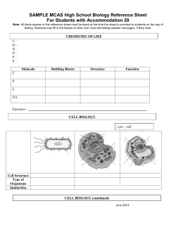


© Copyright 2026