
Master Thesis - University of Twente Student Theses
March 27, 2015
MASTER THESIS
Specifying the WaveCore
in CλaSH
Ruud Harmsen
Faculty of Electrical Engineering, Mathematics and Computer Science (EEMCS)
Computer Architecture for Embedded Systems (CAES)
Exam committee:
Dr. Ir. J. Kuper
Ing. M.J.W. Verstraelen
Ir. J. Scholten
Ir. E. Molenkamp
ABSTRACT
New techniques are being developed to keep Moore’s Law alive, that
is, a doubling in computing power roughly every 2 years. These techniques are mostly focused on parallel programs, this can be the parallelization of existing programs or programs written using a parallel
programming language. A literature study is done to get an overview
of the available methods to make parallel programs. The WaveCore
is an example of a parallel system, which is currently in development. The WaveCore is a multi-core processor, especially designed
for modeling and analyzing acoustic signals and musical instruments
or to add effects to their sound. The WaveCore is programmed with
a graph like language based on data-flow principles. The layout of
WaveCore is not a standard multi-core system where there is a fixed
number of cores connected together via memory and caches. The
WaveCore has a ring like network structure and a shared memory,
also the number of cores is configurable. More specific details about
the WaveCore can be found in the thesis.
A functional approach to hardware description is being developed
at the CAES group at the University of Twente, this is CλaSH. FPGAs are getting more and more advanced and are really suitable for
making parallel programs. The problem with FPGAs however is that
the available programming languages are not really suitable for the
growing sizes and growing complexity of today’s circuits. The idea
is to make a hardware description language which is more abstract
and more efficient in programming than the current industry languages VHDL and Verilog. This abstraction is required to keep big
complex circuit designs manageable and testing can be more efficient
on a higher level of abstraction (using existing model checking tools).
CλaSH is a compiler which converts Haskell code to VHDL or Verilog, the benefits of this are that the Haskell interpreter can be used
as simulation and debug tool.
The focus of this thesis is to specify the WaveCore in CλaSH. Specifying a VLIW processor with CλaSH has been done before, however
because the WaveCore is a non-trivial architecture, it is an interesting
case study to see if such a design is possible in CλaSH. First an implementation is made of a single core of the WaveCore in Haskell. This
is then simulated to prove correctness compared with the existing implementation of the WaveCore. Then the step towards CλaSH is made,
this requires some modifications and adding a pipelined structure (as
this is required in a processor to efficiently execute instructions).
iii
ACKNOWLEDGMENT
This is the final project of my Master "Embedded Systems". The project
had some ups and downs but overall it was a very interesting challenge, during this project I had great help and here I want to thank
people for that. I want to thank my first supervisor Jan Kuper all of
his guidance. This guidance includes reviewing this thesis, discussing
about specific parts of the implementation, providing me with an
interesting project but also for the interesting conversations about
CλaSH and FPGA’s which where not direct part of my research. I
also want to thank my second supervisor, Math Verstraelen, which is
the creator of the WaveCore platform, for his help in answering all
the questions I had about the WaveCore system.
For questions about CλaSH, I would like to thank Christiaan Baaij,
the main creator of CλaSH. My thesis was not the first research in
creating a processor in CλaSH. There was another project where a
processor is designed in CλaSH in the CAES group, this was done by
Jaco Bos and we had some interesting discussions about implementing specific parts, thanks Jaco.
Besides the direct help regarding my thesis by my supervisors and
direct colleagues, I would also like to thank my girlfriend Mara, for
her support during my research. Mara helped me with creating a
good planning, kept me motivated during times things didn’t work
or when I got distracted.
Last but not least I would like to thank my family for supporting and believing in me during my whole educational career, even
though it took some more time than originally planned.
v
CONTENTS
1
2
3
4
5
6
introduction
1
1.1 Background
1
1.2 Parallel Programming models
2
1.3 CλaSH
2
1.4 WaveCore Background
2
1.5 Research Questions
3
1.6 Thesis Outline
3
literature:parallel programming models
5
2.1 Introduction
5
2.2 Programming models
7
2.3 Parallel Systems
9
2.4 FPGAs: Programmable Logic
13
2.5 Conclusion
16
background: the wavecore
17
3.1 Introduction
17
3.2 WaveCore programming language and compiler, simulator
21
3.3 Next Step: Simplified Pipeline (for use with CλaSH)
23
implementation
29
4.1 Introduction
29
4.2 Haskell: A single Processing Unit (PU)
30
4.3 Simulation
37
4.4 Output
39
4.5 Moving to CλaSH
43
results/evaluation
53
5.1 Haskell Simulator vs C Simulator
53
5.2 Problems with developing the Haskell Simulator
54
5.3 CλaSH
54
5.4 Guidelines for Development
56
conclusion
59
6.1 Is CλaSH suitable for creating a multi-core processor
(as example the WaveCore).
59
6.2 What are the advantages and disadvantages using CλaSH
6.3 How does the CλaSH design compare with the existing
design of the WaveCore
60
6.4 Future Work
61
i appendix
63
a haskell/cλash data types
59
65
vii
LIST OF FIGURES
Figure 1
Figure 2
Figure 3
Figure 4
Figure 5
Figure 6
Figure 7
Figure 8
Figure 9
Figure 10
Figure 11
Figure 12
Figure 13
Figure 14
Figure 15
Figure 16
Figure 17
Figure 18
Figure 19
Figure 20
Figure 21
Figure 22
Figure 23
Figure 24
Figure 25
Figure 26
Figure 27
Figure 28
Figure 29
Figure 30
Figure 31
viii
Moore’s Law over time
5
Amdahl’s Law graphical representation
6
Overview of parallel systems
8
OpenMP
9
Multi-core CPU vs GPU
10
CUDA
11
Xilinx Toolflow: From design to FPGA
15
WaveCore Data flow Graph
18
WaveCore Global Architecture
18
WaveCore Processing Unit
20
WaveCore Graph Iteration Unit (GIU) Pipeline
21
WaveCore Load/Store Unit (LSU) Pipeline
21
WaveCore Program Example
22
WaveCore implementation on an Field-Programmable
Gate Array (FPGA)
22
WaveCore Default Instruction
23
WaveCore Initialize Pointers Instruction
23
WaveCore Alternative Route Instruction
24
Simplified Pipeline
25
Impulse response of an Infinite Impulse Response (IIR) filter with a Dirac Pulse as input.
27
WaveCore Processing Unit
30
A mealy machine.
34
Example browser output Haskell-Simulator
40
WaveCore Usage Workflow
40
Preferred Workflow
41
CλaSH RAM usage with generating VHDL
44
FPGA area usage of a single PU with no Block
Ram (Block-RAM) and no pipelining.
45
Registers marked in the Pipeline
48
Values pass through multiple stages
49
Linear increase of memory usage
54
Memory usage fixed
55
Preferred Work-flow
61
LISTINGS
Listing 1
Listing 2
Listing 3
Listing 4
Listing 5
Listing 6
Listing 7
Listing 8
Listing 9
Listing 10
Listing 11
Listing 12
Listing 13
Listing 14
Listing 15
Listing 16
Listing 17
Listing 18
Listing 19
Listing 20
Listing 21
Listing 22
Listing 23
Listing 24
Listing 25
Listing 26
Dirac Pulse in the WaveCore language
26
IIR filter in the WaveCore language
27
Haskell GIU Instructions
31
GIU opcode in Haskell
31
Haskell implementation of the Address Computation Unit (ACU)
32
Haskell implementation of the Arithmetic Logic
Unit (ALU)
33
Alternative Haskell implementation of the ALU
using pattern matching
33
Haskell implementation of the Program Control Unit (PCU)
34
Haskell state definition
35
Haskell implementation of part of the Processing Unit (PU)
37
The simulate function in Haskell for simulation of the HaskellPU
38
Part of the instructions generated from the CSimulator object file
39
Haskell-Simulator output generation
42
Haskell-Simulator output
42
VHDL v1
43
Time to generate VHDL using CλaSH
44
Declaration of the Block-RAM for the GIU Instruction Memory and the X Memory
46
Example code for the execution of Pipeline Stage
2
47
CλaSH code for pipeline stage 2 and 3
48
Multiple stage pass through CλaSH data types
50
Passing through memory addresses over multiple stages
50
Connecting the pipeline stage 2 and 3 together
51
Instruction type definitions
65
Haskell and CλaSH Numeric types
66
CλaSH Datatypes for the Stages(Inputs)
66
CλaSH Datatypes for the Stages(Outputs)
67
ix
ACRONYMS
ACU
Address Computation Unit
ADT
Algebraic Data Type
ALU
Arithmetic Logic Unit
API
Application Programming Interface
ASIC
Application Specific Integrated Circuit
Block-RAM
Block Ram
C++ AMP
C++ Accelerated Massive Parallelism
CAES
Computer Architecture for Embedded Systems
C-Mem
Coefficient Memory
CPU
Central Processing Unit
CSDF
Cyclo-Static Data-flow
CUDA
Compute Unified Device Architecture
DLS
Domain Specific Language
DMA
Memory Controller
DSP
Digital Signal Processor
EDA
Electronic Design Automation
FDN
Feedback Delay Network
FPGA
Field-Programmable Gate Array
GIU
Graph Iteration Unit
GIU Mem
GIU
Instruction Memory
GIU PC
GIU
Program Counter
GPGPU
General Purpose Graphics Processing Unit (GPU)
GPN
Graph Partition Network
GPU
Graphics Processing Unit
HDL
Hardware Description Language
HPC
High Performance Computing
x
acronyms
HPI
Host Processor Interface
ibFiFo
Inbound FiFo
IIR
Infinite Impulse Response
ILP
Instruction-Level Parallelism
IP
Intellectual Property
LE
Logic Element
LSU Load PC
LSU
LSU
Load/Store Unit
LSU Mem
LSU
MIMD
Multiple Instruction Multiple Data
MPI
Message Passing Interface
obFiFo
Outbound FiFo
OpenMP
Open Multi-Processing
PA
Primitive Actor
PCU
Program Control Unit
Pmem
Program Memory
PSL
Property Specification Language
PTE
Primitive Token Element
Pthreads
POSIX Threads
PU
Processing Unit
SFG
Signal Flow Graph
SIMD
Single Instruction Multiple Data
SoC
System on Chip
LSU Store PC
LSU
TLDS
Thread-level Data Speculation
VLIW
Very Large Instruction Word
WBB
WriteBack Buffer
WP
WaveCore Process
WPG
WaveCore Process Graph
Load Program Counter
Instruction Memory
Store Program Counter
xi
xii
acronyms
WPP
WaveCore Process Partition
X-Mem
X Memory
Y-Mem
Y Memory
1
INTRODUCTION
1.1
background
In our everyday live we can not live without computers. Computers and/or Embedded Systems control our lives. But our increasing
need of computing power is stressing all the limits. Around 1970 Gordon Moore[23] noticed that the number of transistors per area die
increased exponentially. This growth is approximated as a doubling
in the number of transistors per chip every two years and therefore an
doubling of computing power as well. This growth later was called
"Moore’s Law". To keep the computational growth of Moore’s Law,
another solution has to be found. A very promising solution to this
problem is the use of multi-core systems. Tasks can be divided over
multiple processors and thus gain the increase in computation power
which conforms with Moore’s Law. But dividing tasks across multiple processors is not an easy task. When a task is divided into as
small as possible subtasks, the execution time then depends on the
tasks which is the slowest (assuming all tasks available are executed
in parallel). As a simple example there are 3 tasks (with a total time
of 9 seconds):
• Task 1 takes 3 seconds to complete
• Task 2 takes 1 second to complete
• Task 3 takes 5 seconds to complete
The total execution time is not the average time of those 3 tasks ( 39 = 3
seconds), but it is 5 seconds because of Task 3. This maximum improvement on a system is called "Amdahl’s Law"[15]. A solution to
this might be to improve the performance of Task 3. This can be done
by making custom hardware for this specific case in stead of using
a generic CPU. Programming languages to create such hardware are
VHDL and Verilog. These are very low level and don’t use a lot of
abstraction. For big designs this is a very time consuming process
and very error prone (Faulty chip design causes financial damage of
$475,000,000 to Intel in 1995[31]). A less error prone and more abstract language is required to reduce the amount of errors and keep
the design of large circuits a bit more simple. This is where CλaSH
comes in. This research will dive in the use of CλaSH as a language
to create a multi-core processor.
1
2
introduction
1.2
parallel programming models
A solution to keep Moore’s Law alive is to go parallel. Creating parallel applications or changing sequential applications to be more parallel is not perfected yet. Research in parallel systems and parallel
programming models are a hot topic. The Graphics Processing Unit,
an Field-Programmable Gate Array and a Multi-core processor are
examples of parallel systems. Each with their advantages and disadvantages. What can be done with them and how to program them is
discussed in Chapter 2.
1.3
cλash
Within the chair CAES the compiler CλaSH is developed which can
translate a hardware specification written in the functional programming language Haskell into the traditional hardware specification language VHDL (and Verilog). It is expected that a specification written
in Haskell is more concise and better understandable than an equivalent specification written in VHDL, and that CλaSH may contribute
to the quality and the correctness of designs. However, until now
only few large scale architectures have been designed using CλaSH,
so experiments are needed to test its suitability for designing complex
architectures.
1.4
wavecore background
The WaveCore is a multi-core processor, especially designed for modeling and analyzing acoustic signals and musical instruments, and to
add effects to their sound. Besides that, the WaveCore is programmed
with a graph like language based on data-flow principles. The layout
of the processor is also not a standard multi-core system where there
is a fixed number of cores connected together via memory and caches.
The WaveCore has a ring like network structure and a shared memory,
also the number of cores is configurable. Because the WaveCore has
a non-trivial architecture it is an interesting target to be modeled in
Haskell/CλaSH. This is not the first processor being developed using
CλaSH. A Very Large Instruction Word (VLIW) processor is developed
using CλaSH in [6]. This research was also done in the CAES group
at the University of Twente. Collaboration and discussions have been
carried out almost every week. More details of the WaveCore can be
found in Chapter 3.
1.5 research questions
1.5
research questions
The idea of this research is to see if CλaSH is usable for specifying the
WaveCore processor. While doing this, the following research questions will be answered.
1. Is CλaSH suitable for creating a non-trivial multi-core processor
(e.g. the WaveCore)?
2. What are the advantages and disadvantages using CλaSH as a
hardware description language?
3. How does the CλaSH design compare with the existing design
of the WaveCore (C Simulator and VHDL hardware description)?
These questions will be answered in Chapter 6.
1.6
thesis outline
This thesis starts with a small literature study (Chapter 2) in the field
of parallel programming models. As can be read in this introduction
is that the future is heading towards more parallel systems (or multicore systems). This parallelization requires a different approach than
the traditional sequential programming languages. After this a chapter is devoted to the many-core architecture of the WaveCore (Chapter
3). This will go in depth to the WaveCore architecture and will make
a start on how this will be implemented in Haskell. The chapter following the WaveCore is the implementation in Haskell and CλaSH
(Chapter 4). After that there will be an explanation of the do’s and
don’t of developing a processor in CλaSH (Chapter 5). This thesis is
finalized by a conclusion in Chapter 6.
3
L I T E R AT U R E : PA R A L L E L P R O G R A M M I N G M O D E L S
2.1
introduction
Computers are becoming more powerful every year, the growth of
this computing power is described by Gordon E. Moore’s[23]. This
growth is approximated as a doubling in the number of transistors
per chip every two years and therefore an doubling of computing
power as well. Figure 1 shows this trend. Most of the time this growth
Figure 1: Moore’s Law over time
is due to reducing the feature size of a single transistor, but during
some periods, there were major design changes[34, 21]. The growth
in computing power can not continue with current techniques. The
transistor feature size is still decreasing, however the associated doubling of computation power is not easy to meet, this is the result of
"hitting" several walls:
• Memory Wall - Access to memory is not growing as fast as the
Central Processing Unit (CPU) speed
• Instruction-Level Parallelism (ILP) Wall - The increasing difficulty of finding enough parallelism in a single instruction stream
to keep a high-performance single-core processor busy
5
2
6
literature:parallel programming models
• Power Wall - A side effect of decreasing the feature size of a
transistor is an increase in the leakage current, this results in
a raise in power usage and thus in an increase of temperature
which is countered by a decrease in clock speed (which slows
down the processor)
A solution to keep this growth in computing power is the parallel approach. Parallel computing on the instruction level is done already in VLIW processors, but these get too complicated due to the
ILP wall[22]. So a more generic parallel approach is required. Creating parallel programs is not trivial (e.g. due to data dependencies)
and converting sequential programs to parallel programs is also not
an easy task. The gain in speedup of converting a sequential program
to a parallel program is also known as Amdahl’s Law [15]. It states
that the maximum speedup of a program is only as fast as it’s slowest
sub part of the program. As an example: when a program takes up
10 hours of computing time on a single core and most of the program
can be parallelized except for one part which takes up 1 hour of computing time (which means 90% parallelization). The resulting parallel
program will still take at least 1 hour to complete, even with infinite
amount of parallelization. This is an effective speedup of (only) 10
times (at a core count of 1000+ see Figure 2), it does not help to add
more cores after a 1000. It shows that the speedup of a program is limited to the parallel portion of the program. With 50% parallelization
only a speedup of 2 times can be achieved.
Figure 2: Amdahl’s Law graphical representation
automatic parallelization Efforts are put into the automatic
parallelization of sequential programs, if this would work correctly, it
2.2 programming models
would be an easy option to make existing sequential programs parallel. One of the techniques to make this possible is Thread-level Data
Speculation (TLDS)[24, 32], this technique speculates that there are no
data dependencies and continue execution until a dependency does
occur and then restart execution. TLDS can accelerate performance
even when restarting is required, as long as it doesn’t have too much
data dependency conflicts.
parallel programming To make better use of the parallel systems, a programming language is required to make this possible. Several programming languages and models exist, these are explained
during this literature study.
current trends Digital Signal Processors (DSPs) gained more
importance in this growing era of multi-core systems[17]. The main
reason is that computational cores are getting smaller so more of
them fit on the same chip, more room for on-chip memory and I/O
operations became more reasonable. Programming these multi-core
systems is still very challenging, therefore research is done to make
this easier. This is done by creating new programming languages (e.g.
[5, 26]) or adding annotations to existing languages.
2.1.1
Literature outline
An introduction to the problem of Moore’s Law is given already. Section 2.2 will give an overview of the currently available parallel programming models. Systems which could benefit from these programming models can be found in Section 2.3, this can range from a single
chip, to a distributed network of systems connected via the Internet.
A further research is done in programming models which are designed to run on programmable hardware like an FPGA in Section 2.4.
This connects with the rest of the Thesis because this is focused on
implementing a multi-core processor on an FPGA using the functional
language Haskell.
2.2
programming models
A detailed summary about all programming models is given in [10,
18]. Figure 3 is a graphical representation of the available models.
This includes the following programming models:
• POSIX Threads (Pthreads) - Shared memory approach
• OpenMP - Also a shared memory approach, but more abstract
than the Pthreads
• MPI - Distributed memory approach
7
8
literature:parallel programming models
Shared Memory
POSIX Threads
OpenMP
CUDA (language)
Distributed Memory
MPI
UPC (language)
Fortress (language)
Cluster
SMP/
MPP
SMP/
MPP
SMP/
MPP
SMP/
MPP
SMP/MPP = These are systems with multiple processors which
share the same Memory-bus
Figure 3: Overview of parallel systems
2.2.1
POSIX Threads
The Pthreads, or Portable Operating System Interface(POSIX) Threads,
is a set of C programming language types and procedure calls[7].
It uses a shared memory approach, all memory is available for all
threads, this requires concurrency control to prevent race conditions.
These types and procedures are combined in a library. The library
contains procedures to do the thread management, control the mutualexclusion(mutex) locks (which control concurrent data access on
shared variables) and the synchronization between threads. The downside of this approach is it is not really scalable, when more threads
are used, accessing shared variables gets more and more complicated.
Another limitation is that it is only available as a C library, no other
languages are supported.
2.2.2
OpenMP
Open Multi-Processing (OpenMP) is an API that supports multi-platform
shared memory multiprocessing programming in C, C++ and
Fortran[9]. Compared to the Pthreads, OpenMP has a higher level of abstraction and support for multiple languages. OpenMP provides the
programmer a simple and flexible interface for creating parallel programs, these programs can range from simple desktop programs, to
programs that could run on a super computer. The parallel programming is achieved by adding annotations to the compiler, thus requiring compiler modification. Can be combined to work with MPI (next
subsection). It uses a shared memory approach just as the Pthreads. An
graphical representation of the multi-threading of OpenMP is showed
in Figure 4, where the Master thread can fork multiple threads to
perform the parallel tasks.
2.3 parallel systems
Figure 4: OpenMP
2.2.3
MPI
Message Passing Interface (MPI) is a distributed memory approach.
This means that communication between threads can not be done by
using shared variables, but by sending "messages" to each other[28].
Compared to OpenMP and Pthreads is more of a standard than a real implantation as a library or compiler construction. The standard consists
of a definition of semantics and syntax for writing portable messagepassing programs, which is available for at least C, C++, Fortran and
Java. Parallel tasks still have to be defined by the programmer (just
as the OpenMP and Pthreads). It is the current standard in High Performance Computing (HPC).
2.3
parallel systems
Now that we have explained some Parallel Models, we dive into systems specifically designed for parallel programming. A parallel system can have multiple definitions. Examples of parallel systems are:
• Multi-Core CPU - Single chip which houses 2 or more functional
units, all communication between cores is done on the same
chip (shown on the left side in Figure 5).
• GPU - A processor designed for graphics which has many cores,
but these cores are more simple then a MultiCore CPU shown
on the right in Figure 5.
• FPGA - An FPGA is a chip that contains programmable logic
which is much more flexible then a GPU or CPU, but the clock
speed is much lower than that of a GPU or CPU.
• Computer Clusters (Grids) - Multiple computers can be connected together to perform calculations, synchronization is not
easy and most of the time the bottleneck of these systems
(SETI@Home is an example currently used for scanning the
galaxy for Extraterrestrial Life[1]).
9
10
literature:parallel programming models
Control
ALU
ALU
ALU
ALU
Cache
DRAM
DRAM
GPU
CPU
Figure 5: Multi-core CPU vs GPU
2.3.1
GPU
are massively parallel processors. They are optimized for Single Instruction Multiple Data (SIMD) parallelism, this means that a
single instruction will be executed on multiple streams of data. All
the processors inside a GPU will perform the same task on different
data. This approach of using the processors inside a GPU is called
General Purpose GPU (GPGPU) [12, 19, 29, 30, 33]. The GPU has a parallel computation model and runs at a lower clock rate than a CPU.
This means that only programs which perform matrix or vector calculations can benefit from a GPUs. In video processing this is the case
because calculations are done on a lot of pixels at the same time.
Programming languages to make applications for the GPU are:
GPUs
1. CUDA - Developed by NVIDEA[27] and only works on NVIDEA
graphic cards.
2. OpenCL - Developed by Apple[14] and is more generic than
CUDA and is not limited to only graphic cards.
3. Directcompute and C++ AMP - Developed by Microsoft and
are libraries part of DirectX 11, only works under the windows
operating system.
4. Array Building Blocks - Intel’s approach to parallel programming (not specific to GPU).
Compute Unified Device Architecture (CUDA)
is developed by NVIDEA in 2007[27]. An overview of CUDA is
given in Figure 6. It gives developers direct access to virtual instruction set and the memory inside a GPU (only NVIDEA GPUs). CUDA
is a set of libraries available for multiple programming languages, including C, C++ and Fortran. Because CUDA is not a very high level
language, it is not easy to develop programs in it. Developers would
like to see high level languages to create applications (which makes
CUDA
2.3 parallel systems
Figure 6: CUDA
development faster and easier). Therefore research is done in generating CUDA out of languages with more abstraction. Examples are:
• Accelerate[8] - Haskell to CUDA compiler
• PyCUDA[20] - Python to CUDA compiler
accelerate Research has been done to generate CUDA code out
of an embedded language in Haskell named Accelerate[8]. They state
that it increases the simplicity of a parallel program and the resulting code can compete with moderately optimized native CUDA code.
Accelerate is a high level language that is compiled to low-level GPU
code (CUDA). This generation is done via code-skeletons which generate the CUDA code. It is focused on Array and Vector calculations,
Vectors and Arrays are needed because the GPU requires a fixed
length to operate (it has a fixed number of cores), thus making Lists in
Haskell unusable. Higher order functions like map and fold are rewritten to have the same behavior as in Haskell. This has still the abstractions of Haskell, but can be recompiled to be CUDA compatible. A
comparison is made with an vector dot product algorithm, what was
observed is that the time to get the data to the GPU was by far the
limiting factor. (20 ms to get the data to the GPU and 3,5ms execution
time with a sample set of 18 million floats). The calculation itself was
much faster on the GPU than on the CPU (about 3,5 times faster, this
includes the transfer time for the data).
11
12
literature:parallel programming models
fcuda Although CUDA programs are supposed to be run on a
GPU, research is being done to compile it to FPGA’s. This is called
FCUDA [29]. Their solution to keep Moore’s Law alive is to make it
easier to write parallel programs for the FPGA using CUDA. FCUDA
compiles CUDA code to parallel C which then can be used to program an FPGA. CUDA for the FPGA is not enough according to
them for more application specific algorithms which cannot exploit
the massive parallelism in the GPU and therefore require the more reconfigurable fabric of an FPGA. Their example programs show good
result especially when using smaller bit-width numbers than 32-bit,
this is because the GPU is optimized for using 32-bit numbers. Programs which use more application specific algorithms should perform much better on the FPGA than on the GPU, this was not tested
thoroughly yet.
OpenCL
OpenCL is a framework for writing programs that run on heterogeneous systems, these systems consist of one or more of the following:
• Central Processing Units (CPUs)
• Graphics Processing Units (GPUs)
• Digital Signal Processors (DSPs)
• Field-Programmable Gate Arrays (FPGAs)
OpenCL is based on on the programming language C and includes
an Application Programming Interface (API). Because OpenCL is not
only a framework for an GPU, it also provides a task based framework
which can be for example run on an FPGA or CPU. OpenCL is an
open standard and supported by many manufacturers. Research is
done in compiling OpenCL to FPGA’s to generate application specific
processors[16].
DirectCompute
DirectCompute is Microsoft’s approach to GPU programming. It is
a library written for DirectX and only works on the newer windows
operating systems.
Array Building Blocks
Intel’s approach to make parallel program easier is done in [25]. Their
aim is a retargetable and dynamic platform which is not limited to
run on a single system configuration. It is mostly beneficial in data
intensive mathematical computation and should be deadlock free by
design.
2.4 fpgas: programmable logic
Heterogeneous systems
2.3.2
The methods mentioned until now mostly use 1 kind of system. In
heterogeneous systems there could be multiple types of parallel systems working together. CUDA is a heterogeneous system because it
uses the GPU in combination with the CPU. A whole other kind of heterogeneous system is a grid computing system. Multiple computers
connected via a network working together is also a heterogeneous
system. An upcoming heterogeneous system is the use of FPGA together with a CPU. The FPGA can offload the CPU by doing complex
parallel operations. Another possibility of the FPGA is that it can be
reconfigured to do other tasks. More about the FPGA is in the next
section.
2.4
fpgas: programmable logic
once were seen as slow, less powerful Application Specific Integrated Circuit (ASIC) replacements. Nowadays they get more and
more powerful due to Moore’s Law[4]. Due to the high availability
of Logic Elements (LEs) and Block-RAMs and how the Block-RAM is distributed over the whole FPGA, it can deliver a lot of bandwidth (a
lot can be done in parallel, depending on the algorithm run on the
FPGA). Although the clock-speed of an FPGA is typically an order of
magnitude lower than a CPU, the performance of an FPGA could be a
lot higher in some applications. This higher performance in an FPGA
is because the CPU is more generic and has a lot of overhead per instruction, where the FPGA can be configured to do a lot in parallel.
The GPU however is slightly better in calculation with Floating Point
numbers, compared with the FPGA. The power efficiency however is
much lower on an FPGA compared with a CPU or GPU, research on
this power efficiency of an FPGA has been done in several fields and
algorithms (e.g. Image Processing [30], Sliding Window applications
[12] and Random Number generation [33]). The difference in performance between the CPU and FPGA lies in the architecture that is used.
A CPU uses an architecture where instructions have to be fetched from
memory, based on that instruction a certain calculation has to be done
and data which is used in this calculation also has to come from memory somewhere. This requires a lot of memory reading and writing
which takes up a lot of time. The design of the ALU also has to be
generic enough to support multiple instructions, which means that
during execution of a certain instruction, only a part of the ALU is active, which could be seen as a waste of resources. An FPGA algorithm
doesn’t have to use an instruction memory, the program is rolled out
entirely over the FPGA as a combinatorial path. This means that most
of the time, the entire program can be executed in just 1 clock cycle.
Therefore an algorithm on the FPGA could be a lot faster when it
FPGAs
13
14
literature:parallel programming models
fit’s on an FPGA and takes up a lot of clock cycles on the CPU. This
is not the only reason an FPGA could be faster, the distributed style
of the memory on an FPGA can outperform the memory usage on
an CPU easily. Because the memory on an FPGA is available locally
on the same chip near the ALU logic, there is almost no delay and
because there are multiple Block-RAM available on an FPGA, the data
could be delivered in parallel to the algorithm. The big downside of
using FPGAs is the programmability, this is not easily mastered. The
current industry standards for programming an FPGA are VHDL and
Verilog. These are very low level and the tools available are not easily used as well Figure 7 shows the tool-flow when using the Xilinx
tools. Fist a design in VHDL or Verilog has to be made, this design
is then simulated using the Xilinx tools. When simulation is successful, the design can be synthesized. This synthesization can take up
to a few seconds for small designs but bigger design synthesization
could take up to a couple of days. Then optimization steps will be
done by the tool followed by mapping, placement and routing on the
FPGA. This results in a net list file which then can be used to program
the FPGA. The steps from synthesis to programming the FPGA could
not be improved much, what can be improved is the programming
language. Another downside of using VHDL or Verilog is that FPGA
vendors have specific Intellectual Property (IP) cores which are not
hardly interchangeable between FPGAs of the same vendor and even
worse compatibility between vendors. That is the subject for the final
part of this literature study.
2.4.1
High level programming of the FPGA
As mentioned before, the current standards for programming the
FPGA are VHDL and Verilog, these are low level languages and higher
level languages are preferred for easier development and better scalability. Doing simulation with VHDL and Verilog requires Waveform
simulation which is doable for small designs, but get exponentially
complicated with bigger designs, this makes verification hard. Research is being done to compile different high level languages to
VHDL or Verilog. The goal of these languages is to leave out the
step of WaveForm simulation. Another benefit of using high level languages is the support for existing verification tools. VHDL has some
tools for verification but are not easy to use (e.g. Property Specification Language (PSL)). A couple of methods to generate VHDL are:
• System Verilog - A more object oriented version of Verilog, but
this is not very well supported by current Electronic Design
Automation (EDA) tools
2.4 fpgas: programmable logic
Figure 7: Xilinx Toolflow: From design to FPGA
• C-Based frameworks - A couple of frameworks are available for
compiling a small subset of C to VHDL but are very limited (e.g.
no dynamic memory allocation)
• CUDA/OpenCL - These are already parallel languages and
should be more compatible with the parallel nature of an FPGA
but the languages used are still low level (C, C++, Fortran)
• High Level Languages - These are more abstract and could use
existing tools for verification, some examples will be given in
the next section
• Model Based - There are compilers available which can convert
Matlab or Labview to VHDL or Verilog, or the use of data-flow
graphs as in [26] can be used to program DSP like algorithms on
the FPGA
15
16
literature:parallel programming models
2.4.2
High Level Languages
As mentioned as one of the solutions for better programmability of
the FPGA is the use of high level programming languages. A few languages will be mentioned here.
cλash One of these languages is CλaSH [3], this is a language
based on Haskell in which a subset of Haskell can be compiled to
VHDL and Verilog. This language is being developed at the Computer Architecture for Embedded Systems (CAES) group on the University of Twente. Haskell’s abstraction and polymorphism can be
used by CλaSH. Usage of lists and recursion however is not supported in CλaSH, this is because hardware requires fixed length values. A functional programming language (Haskell) is used because
this matches hardware circuits a lot better than traditional sequential
code. This is because a functional language is already a parallel language. Once a circuit is designed and simulated in CλaSH, the code
can be generated for the FPGA. Currently both VHDL and Verilog
are supported. Another language which uses Haskell as a base for
designing digital circuit is Lava [13].
liquidmetal Another language to program FPGAs or more general, heterogeneous systems, is Lime[2]. Lime is compiled by the LiquidMetal compiler. It has support for polymorphism and generic type
classes. Support for Object oriented programming is also included,
this complies with modern standards of programming and is common knowledge of developers. Another approach using LiquidMetal
is the use of task based data-flow diagrams as input to the compiler.
LiquidMetal is not specifically targeted for FPGAs, it can be used on
the GPU as well. When using the FPGA, the LiquidMetal compiler will
generate Verilog.
2.5
conclusion
technology is getting much more interesting due to the increase
of transistor count and features available on the FPGA. Programming
the FPGA however using the current standards, VHDL and Verilog, is
getting to complex. Waveform simulation of big designs is not feasible anymore therefore more abstraction is required. Using high level
languages seems to be the direction to go in the FPGA world. Simulation can be done using the high level languages in stead of using
Waveform simulation, this can be much faster and existing verification tools can be used. CλaSH is a good example of using a functional
languages as a Hardware Description Language (HDL). The EDA tools
currently available can use an update as well, support for more languages is preferred, but that is out of the scope of this research.
FPGA
3
B A C K G R O U N D : T H E WAV E C O R E
3.1
introduction
The WaveCore is a coarse-grained reconfigurable Multiple Instruction
Multiple Data (MIMD) architecture ([35], [36]). The main focus is on
modeling and analyzing acoustic signals (generating the sound of e.g.
a guitar string or create filters on an incoming signal.) The WaveCore
has a guaranteed throughput, minimal (constant) latency and zero
jitter. Because of the constant minimal latency, there is no jitter. This
is important in audio signal generation because the human ear is very
sensitive to hiccups in audio. This chapter will explain the software
and hardware architecture of the WaveCore and some pointers to the
CλaSH implementation are made at the end.
3.1.1
Software Architecture
The software architecture is based on data-flow principles. Figure 8
shows a schematic representation of the data-flow model. The toplevel consists of one or more actors called WaveCore Processes (WPs),
a graph can consist of multiple WPs interconnected via edges. These
edges are the communication channels between WPs. Each WP consist
of one or partitions. Every partition is broken down to multiple Primitive Actors (PAs). These PAs are interconnected via edges, at most 2
incoming edges and 1 outgoing edge. The tokens on these edges are
called Primitive Token Elements (PTEs). Each PA is fired according to a
compile-time derived static schedule. On each firing, a PA consumes
2 tokens and produces 1 token. The output token can delayed using the delay-line parameter. A delay-line is an elementary function
which is necessary to describe Feedback Delay Networks (FDNs), or
Digital Waveguide models. This delay can be used for e.g. adding
reverberation to an input signal or adding an echo.
3.1.2
Hardware Architecture
The introduction showed the programming model of the WaveCore
processor. This section will show how this is mapped to hardware.
The global architecture of the WaveCore is show in Figure 9. This
consist of a cluster of:
• Multiple Processing Units (PUs) (explained in the next section)
17
18
background: the wavecore
o input data available, resulting
ptimization mechanism. Each
n-cached local memory which
that many common DSP tasks
ent. A streaming application is
r a number of dataflow driven
methodology is based on C,
osed to the programmer. Our
me of the aspects of the menFigure
flowgraph
Graph
Fig. 8:
1. WaveCore
WaveCoreData
dataflow
C processor core, scalability of
edge data-flow). However, we
piler,
elay-line length modulation edge
mming
methodology instead of
is illustrated in fig. 1 by edge E1, which tokens are split and
length
us on very strict predictability
dge
forwarded to WP-partitions WP1.a and WP1.b. The concept
h is dominantly driven by the
dge
of WP-partitions is driven by the MIMD architecture, where a
acoustical
modeling.
Incmp,
section
function (add,
mul, div,
etc.) WP might be decomposed and mapped on multiple processing
ore
programming
methodology
(applicable
when required
by f , e.g.
entities as we will show in the next section of this paper.
n p.x
section
=
1 [n]) IV. we position the
Ultimately a WP-partition breaks down into one or more
technology in section V. and
erent delay-line support within the ’primitive actors’ (PA). Hence, a WP, or WP-partition consists
inspired by physical modeling of of an arbitrary number of arbitrarily connected PAs. Likewise,
Figure partition)
9: WaveCorebreaks
Global Architecture
down into one or more
. TheARCHITECTURE
delay-line as a basic modeling a token (or token
MD
Fig. 3. WaveCore MIMD cluster
tal role within this domain. Adding atomic ’primitive token elements’ (PTE). Each PA in a WP
the WaveCore
prohoduction
to this concept
efficiently extends
is• unconditionally
fired
to a compile-time
derived
External memory,
the according
WaveCore drives
a high-performance
inked
to the
MIMD
architecture
s with
a wide
range
of dynamic static
schedule
when
the
WP
itself
is
fired.
Upon
firing,
a
PA
terface
could and
be linked
to one
for example
controller
each
PU which
can produce
consume
graph-cuta PTE
each for
ion domain.
Themulti-path
programming
Doppler
shifting,
delay in consumes
DRAM
or
a
controller
connected
to
a
PCIe
device.
at
most
two
PTEs
and
produces
one
PTE.
A PA
clock cycle. Tokens which are produced by PAs remain inside
representation
of a cyclo-static
ms,
etc.). The supported
arithmetic
is the
a 6-tuple
in fig.is mapped,
2. Uponunless
firingthese
the PA
PU ontowhich
which is
thedepicted
WP(partition)
The Host Processor Interface (HPI) which handles the initializaed
withwill
the show
’f ’ tuple-element)
s we
this conceptare •tokens
are associated to delay-lines, graph-cuts or WP-edge
tion of the cluster (writing the instruction memories of the PUs)
asic
arithmetic
logical model
functions
pping
of the and
data-flow
tokens. The memory hierarchy is derived from the locality of
cation,
division,
and provides runtime-control to the cluster.
well as multiply-addition,
a natural programming
reference properties of a WaveCore CSDF graph. Within the
haves
combinatorial
when
Λ
equals
es. The MIMD architecture is
hierarchy we distinguish three levels, without caches. Level1
n Λ is unequal to zero. As a result, • The Cyclo-Static Data-flow (CSDF) scheduler periodically fires
isevery
associated
to inlocal
memory references
which(WPG
are )due
to
ed
to the programming model.
process
the WaveCore
Process Graph
according
s an abstract RTL (Register Transfer
the
of PAs
within
a WP-partition.
The required
te on the dataflow model, folto aexecution
compile-time
derived
static
schedule.
a WP is a network of interconnected
storage
capacity
for
this
execution
is
located
inside
each PU as
associated
MIMD architecture.
ntial
basic elements.
The RTL nature
tightly coupled data memory. The ’mem’ tile within the cluster
for the WaveCore MIMD processor This cluster is scalable, the number of PUs is configurable (as long as
thethe
level2
memory
dominantly
associated to
thereembodies
is room on
target
device,and
this is
could
be an Field-Programmable
tioning of the technology as we will
token buffering and Application
delay-line
data
storage.
Apart from
that,
Specific
Integrated
Circuit
(ASIC)).
2. Primitive
Actor
(PA)
of a WaveCore dataflow graph Gate Array (FPGA) or anFig.
the level-2 memory tile is used to support PA execution (e.g.
el, the graph consists of actors,
transcendental
functions
likeRISC
hyperbolic,
where the
unitlook-up
Eachon
PUits
is afunction
small
consumes (depending
f ) processor.
at most two PTEs
Dcesses
cluster(WP), and edges. WPs processing
associated
physical
look-up
table
is
shared
by
all
PUs
in
Every
WaveCore
Process
Partition
(WPP
) is
mapped
to
a order
single an
PU.
(carried
by
inbound
edges
x
[n]
and
x
[n])
and
produces
1
2
er
via
tokens
which
are
transto
avoid
replication
of
relatively
expensive
look-up
memory
model can be mapped on a reconfigThis
mapping
done automatically
by the
compiler.
The PUs are
conoutput
PTEinisthrough
thePUoutbound
edge
withlevel2
optional
delayis
periodically
according
resources
each
PU).
to the
shared
memory
cluster,
which isfired,
depicted
in fig. 3.
nected
via a ring
network
andaccess
have access
to a shared
memory.
line
λ], according
to equation
1. arbitration scheme. The
tiley[n
isof+
arbitrated
by
means
of
a
fixed
sistsdoes
of anot
matrix
of interconnected
WP
autonomously
fire structure
a single PU is showed in Figure 10. The different blocks
Conflicting level2 memory access is self-scheduled through
and input
a localedge(s)
shared memory
ns, its
but in tile.
an A
of the PU are explained in section 3.3. Every PU consist of a Graph
λ] = f (x
x [n],top)be resolved by (1)
and+therefore
not1 [n],
required
rocessor,
which is The
optimized
for WP HW arbitration y[n
ntral scheduler.
rationale
Iteration Unit (GIU) and a Load/Store
Unit 2(LSU). The GIU is the main
d in yields
more detail
in the
next section. the mapping tools. All remaining level3 memory traffic is
this
a strict,
predictable
calculation unit, has it own memories and control logic. The LSU takes
mapped
the externallength
memorycan
interface.
This level3with
memory
nfigured through the Host Processor Where
theondelay-line
be modulated
the inbehavior. A WP might have
is used
to
store
token
data
as
well
as
large
delay-line
buffer
purpose, a host-CPU (which could be bound
edge τ [n] at run-time, according to equation 2.
edges, where each edge carries
sor) loads a configuration image into space. The difference with level2 memory is that level3 is
edge has
producer,
a large
memory,
programs
theone
CSDF
scheduler.but
This supposed to be λ[n
+ 1]bulk
= bΛ.(τ
[n] −like
1)c DDR3. Level3 (2)
which
enablesperiodically
broadcast-token
timer which
generates memory is also used to exchange tokens between WaveCore
deviation
thewhich
purethe
CSDF
HPI to the from
PUs on
WP, or processes and possibly other processes, like control actors
The PTEs (being floating-point numbers) which are carried by
nd
hence closed-loop
d. Therefore,
each PU hasprocess
to iterate which might be executed as SW process on the host CPU.
inboundthe
edge
τ [n]memory
determine
actualtodelay-line
length λ.
level3
can the
be used
exchange tokens
on
within
the available
time, before
fully
deterministic
because
of theLikewise,
According to equation 2, the actual delay-line length λ varies
3.1 introduction
care of moving external data to/from the executed WaveCoreWPP (token data and/or delay-line data). The LSU has 2 threads which control the communication between the external memory and the GIU,
one thread to store data from the GIU in the external memory (Store
Thread) and one to read data from the external memory to the GIU.
This is done via buffers between the LSU and the GIU. Because of
this of this "decoupling", this hides the memory latency from the GIU
which makes the iteration process more efficient. Components inside
the GIU are:
• Arithmetic Logic Unit (ALU) - The arithmetic computation unit
• X and Y memories - The local memories used by the ALU
• Cmem - The Coefficient Memory, which is required by some
instructions as a third parameter
• Address Computation Unit (ACU) - This unit calculates all the
memory address required to read and write to the X and Y
memory
• Router - Handles the WriteBack of the output of the ALU, this
could be to one of the internal memories, the external memory
or the Graph Partition Network (GPN)
• GPN port - Handles the communication with other PUs.
• WriteBack Buffer (WBB) - Acts as a buffer between for the Coefficient Memory (C-Mem), when the buffer is filled and no other
components are writing to the C-Mem, the WBB will be written
to the C-Mem.
• HPI port - Handles the communication with the host processor
• Program Control Unit (PCU) - Parses the ALU function from the
instruction coming from the Program Memory (Pmem)
• Inbound FiFo (ibFiFo) and Outbound FiFo (obFiFo) - FiFo buffers
for communication between the GIU and LSU
graph iteration unit The pipeline structure of the GIU is
showed in Figure 11. The pipeline in the current configuration consists of 13 stages where most of the stages are required for the execution of the floating point unit (this currently depends on the Xilinx
floating point technology). Below is a summary of the pipeline inner
workings (a more detailed explanation is given in section 3.3). The
instruction set of the GIU is optimized to execute (i.e. fire) a PA within
a single clock-cycle.
• FET - Fetch instructions from the instruction memory
19
20
background: the wavecore
HPI
GIU
GPN
GPN
GPN
port
port
LSU
HPI
HPI
port
port
Xmem
Xmem
Ymem
Ymem
ACU
ACU
PCU
PCU
Pmem
Pmem
DMAC
DMAC
X1
P
ALU
ALU
Cmem
Cmem
X2
f
y[n]
Router
Router
Ext.
Mem
WBB
WBB
ibFIFO
ibFIFO
obFIFO
obFIFO
GIU: Graph Iteration Unit
LSU: Load/Store Unit
Figure 10:
GPN: Graph Partition Network
LSU: Load/Store Unit
PCU: Program Control Unit
ACU: Address Computation Unit
WBB: WriteBack Buffer
WaveCore Processing Unit
• DEC - Decode the instruction and setup reads for the internal
GPN port writeback into X/Y memories:
memories
- Main requirement: predictability => conflicting ports
- Writeback to X/Y memories is in most cases not replicated (either X or Y)
- Use both A and B ports of the memories? => does not make much sense because
• OP
- Read
FiFo=>ifin many
required
Operand
fetch is inoperands
many cases on from
both memories
cases no free timeslots
- Shallow buffer in GPN unit?
- WBB for GIU writeback?
• EXE1
(x4) - inExecute
Floating Point Adder
- Solve completely
compiler:
=> possible?
=> exact known determinism
=> what about predictability in GPN network?
=> forget it........
- Most probable solution:
=> Compiler “soft-schedule”
=> Evenly distributed X/Y memory allocation
=> GPN moves schedule balance: not too early, not very late
=> Shallow buffer in GPN unit
• EXE2 (x6) - Execute Floating Point Multiplier
• WB1 - Write-back of the calculation results
• WB2 - Communicate with the GPN network
load/store unit The LSU executes two linked-lists of DMAdescriptors (one for the load, the other for the store-thread). A DMA
descriptor is composed of a small number of instructions. The LSU
also makes use of a pipeline, this is showed in figure 12.
It consists of 3 simple stages:
• Stage 1 - Fetch the instructions from the Instruction Memory
and update internal registers used for communication with the
external memory
• Stage 2 - Decode instructions
• Stage 3 - Pointer updates are written back to cMem, and external memory transactions are initiated
vs.programming
GIU pipeline language and compiler, simulator
3.2Resources
wavecore
Imem
(A port)
CoefMem
(A port)
CoefMem
WBB
A-port/Dmem
Inbound
FIFO
B-type PA
Writeback
or GPN address read
B-port/Dmem**
Outbound
FIFO
= FET pipeline stage
= DEC pipeline stage
= OP pipeline stage
= EXE1 pipeline stage
= EXE1 pipeline stage
= EXE1 pipeline stage
= EXE1 pipeline stage
= EXE2 pipeline stage
= EXE2 pipeline stage
= EXE2 pipeline stage
= EXE2 pipeline stage
= EXE2 pipeline stage
= EXE2 pipeline stage
= WB1 pipeline stage
= WB2 pipeline stage
GPN initiator
port
Figure 11: WaveCore GIU Pipeline
load PC, store PC
FET
Imem
DEC
Registers
MOV
WBB
Dmem
**) Writeback and GPN address fetch is mutually exclusive (GPN destination has no
local X/Y memory writeback as side effect)
Figure 12: WaveCore LSU Pipeline
3.2
wavecore programming language and compiler, simulator
As mentioned in section 3.1.1, the programming model is based on
the data-flow principle. A program consists of one or more Signal
Flow Graphs (SFGs). Each SFG consist of a list of statements (the instructions). Each statement has the following structure:
< f >< x1 >< x2 >< y >< p >< dl >
where:
• f - The ALU-function
• x1 - Source location of x1
• x2 - Source location of x2
• y - Write-back destination
• p - Location of the 3rd ALU variable
• dl - Delay length
21
22
background: the wavecore
AnCoding
exampleaprogram
with Process
block diagram
WaveCore
(WP)is showed in Figure 13.
Programs
for thethe
WaveCore
can be run/tested with the C-Simulator.
3) Instantiate
PAs
x[n]
b0
+
PA1
y[n]
a
-1
Z
PA5
+
b1
+
c
d
-1
Z
PA3
b2
SFG
Q x[n]
Q x[n]
Q y[n]
M x[n]
Q y[n]
GFS
b
-a1
PA2
a
b
c
void
d
y[n]
a
b
d
c
< b0>
< b1>
<-a1>
< b2>
<-a2>
0
1
0
0
1
PA4
-a2
+
04/30/14
38
Figure 13: WaveCore Program Example
This simulator is written in C. The C-Simulator takes the byte-code
generated by the WaveCore compiler. The WaveCore compiler takes
care of the mapping to the different PUs of efficient execution. An
example implementation which uses 5 PUs is showed in figure 14.
This is implemented on an Spartan 6 LX45 FPGA1 .
platform
Digilent Atlys board
Spartan6 LX45
FPGA
USB2.0
USB/
USB/
RS232
RS232
HPI
HPI
HPI
HPI
Bridge
Bridge
PU
PU
PU
PU
PU
PU
Mem
Mem
PU
PU
PU
PU
DDRController
Controller
DDR
up to 8960 PAs @48 kHz
WaveCore cluster
Ext.Mem
Mem
Ext.
e on Xilinx Spartan®-6 LX45:
128
128MByte
MByte
DDR2
DDR2
hip L1 memory
hip L2 memory
Analog
I/O
DR2 L3 memory
odec
hnology evaluation
AC97
AC97
Audio
Audio
Codec
Codec
Control
Control
Stream
Stream
Actor
Actor
Digital Audio Interface
Figure 14: WaveCore implementation on an FPGA
3.2.1
WaveCore GIU Instructions
processor application demo
TODO: - Opcodes mappen naar WC language?
sical modeling with ultra-low
The WaveCore GIU instructions can be divided into 3 groups:
1 http://www.xilinx.com/products/silicon-devices/fpga/spartan-6/lx.html
03/06/14
12
3.3 next step: simplified pipeline (for use with cλash)
• Default Instructions - These instructions execute most of the
instructions see Figure 15.
• Pointer Initialization Instructions - These instructions initialize the memory pointers which are update by the ACU and used
to address the x and y memories. The structure of this instruction is showed in Figure 16.
• Alternative Route Instruction - These are instructions where
the result of the ALU does not take the normal route, but are
routed trough the GPN or the external memory, see Figure 17.
As can be seen in Figures 15, 16 and 17 is that the length of the
instructions is only 28 bits (0 - 27). The WaveCore however uses 32
bit instructions, the 4 missing bits are reserved for the opcode for the
ALU. The ALU can execute during every instruction mentioned above.
The possible OpCodes are listed in Table 1. The bit representations
of the OpCode are not important for now but can be found in the
WaveCore
documentation.
Default
Default
pointer
mode
27 26
26 25
25 24
24 23
23
27
17 16
16 15
15 14
17
dest a/s
dl dest
a/s
dl
pd(7b)
pd(7b)
oa a/s
oa
a/s
acuX(8b)
acuW(8b)
acuW(8b)
00=X-mem
00=X-mem
01=Y-mem
01=Y-mem
10=XY-mem (repl.)
(repl.)
10=XY-mem
11=Alt-mode
11=Alt-mode
0=no delayline
delayline
0=no
1=delayline
1=delayline
8 7 6
pd(7b)
0
pd(7b)
acuY(8b)
a/s:
0=Add
1=Sub
Operand Memory
Memory Assign:
Operand
X1 →
→ Xmem, X2 → Ymem
00 == X1
X2 →
→ Xmem, X1 → Ymem
11 == X2
pd(7b) == pointer
pointer displacement:
displacement:
bits WaveCore
unsigned number,
number,
to be added
pd(7b)
bits
unsigned
to
to / subtracted from referenced pointer
Figure7715:
Default
Instruction
Alt pointer
pointer mode, pointer init
Alt
27 26
26 25
25 24
24
27
00
11 11
19 18
18
19
12 11
sel
sel
0
not used
used
not
imm
imm(12b)
sel(5)=X-wb
sel(5)=X-wb
sel(4)=Y-wb
sel(4)=Y-wb
sel(3)=PntrGPNx
sel(3)=PntrGPNx
sel(2)=PntrGPNy
sel(2)=PntrGPNy
sel(1)=X-op
sel(1)=X-op
sel(0)=Y-op
sel(0)=Y-op
Alt pointer
pointerFigure
Alt
mode,
alternative
route
(token
and/or GPN)
16: WaveCore
Initialize
Pointers
Instruction
27 26
26 25
25 24
24
27
11
3.3
11 11
22 19
19
22
16 15
15
16
opRC
-opRC
wbRC
wbRC
3b
3b
4b
4b
87
acuX*/acuWa
0
acuY*/acuWb
8b
8b cλash)
8b
8b
next step: simplified pipeline
(for use with
opRC
opRC
X1
X1
X2
X2
WbRC(3:0)
WbRC(3:0)
WB-dest
WB-dest
101
101
110
110
111
111
Y
Y
---
X
X
---
0101
0101
0110
0110
0111
0111
1--1---
Y(b)
Y(b)
XY(b)
XY(b)
IGC(y)
IGC(y)
LSP
LSP
000
X
LSP
0000
X(a)
Now that 000
we have discussed
the
existing WaveCore,0000
a start is made
to
X
LSP
X(a)
001
Y
LSP
0001
Y(a)
001
Y
0001
Y(a)
implement
this in CλaSH.
TheLSP
pipeline is simplified,
namely the
float010
LSP
X
0010
XY(a)
010
LSP
X
0010
XY(a)
ing point 011
arithmeticLSP
is replaced
011
LSP
Y by fixed point. This
0011simplifications
IGC(x)
Y
0011
IGC(x)
100 to implement
X
0100(and in X(b)
X(b)
make it easier
theYY WaveCore in CλaSH
general
100
X
0100
*) acuX/acuY
acuX/acuY format
format is
is identical
identical to
to acuW
acuW or
or acuX/acuY
acuX/acuY format
format (depending
(depending on
on context)
context)
*)
*) Conflicting
Conflicting permutations
permutations between
between opRC
opRC and
and wbRC
wbRC are
are not
not checked
checked by
by HW
HW
*)
*)Assignment
Assignment definition
definition in
in acuX/Y/W
acuX/Y/W fields
fields are
are ignored
ignored in
in 'Alt'-mode
'Alt'-mode
*)
*) WbRC(3)
WbRC(3) == LSU
LSU destination
destination writeback
writeback enable
enable ('1'
('1' ==
== push
push outbound
outbound FIFO)
FIFO)
*)
NOTE: LSU
LSU is
is the
the only
only destination
destination in
in that
that case
case (no
(no parallel
parallel writeback)!!
writeback)!!
NOTE:
*) Delay-lines
Delay-lines are
are not
not supported
supported within
within Alt-pointer
Alt-pointer mode
mode
*)
23
sel(5)=X-wb
sel(4)=Y-wb
sel(3)=PntrGPNx
sel(2)=PntrGPNy
sel(1)=X-op
sel(0)=Y-op the
background:
24
wavecore
Alt pointer mode, alternative route (token and/or GPN)
27
1
26 25 24
1 1
opRC
000
001
010
011
100
101
110
111
22 19
16 15
87
0
opRC
wbRC
acuX*/acuWa
acuY*/acuWb
3b
4b
8b
8b
X1
X
Y
LSP
LSP
X
Y
-
X2
LSP
LSP
X
Y
Y
X
-
WbRC(3:0)
0000
0001
0010
0011
0100
0101
0110
0111
1---
WB-dest
X(a)
Y(a)
XY(a)
IGC(x)
X(b)
Y(b)
XY(b)
IGC(y)
LSP
*) acuX/acuY
format is17:
identical
to acuW or
acuX/acuY format
(depending
on context)
Figure
WaveCore
Alternative
Route
Instruction
*) Conflicting permutations between opRC and wbRC are not checked by HW
*) Assignment definition in acuX/Y/W fields are ignored in 'Alt'-mode
*) WbRC(3) = LSU destination writeback enable ('1' == push outbound FIFO)
OpCode
Function
NOTE:
LSU is the only destination in that case (no parallel writeback)!!
*) Delay-lines are not supported within Alt-pointer mode
ADD
y[n + λ] = x1 [n] + x2 [n]
*) Replicated X/Y writeback uses X-WB pointer solely
*) LSU WB simultaneous
CMP
y[n + λ] with
==Wbrc
(x1modi
[n] NOT
> xpossible
2 [n]) (NOTE: handle in compiler)
*) Writeback is disabled when NOP instructions are executed. However, pointer updates are possible in combination
with NOP instructions.
DIV
y[n + λ] = x [n]/x [n]
1
2
LGF
y[n + λ] = LogicFunct(x1 [n], x2 [n], p
LUT
y[n + λ] = Lookup[x1 [n]]
MUL
y[n + λ] = x1 [n] · x2 [n]
MAD
AMP
RND
y[n + λ] = p · x1 [n] · x2 [n]
y[n + λ] = p · x1 [n]
y[n] = random(0, 1)
Table 1: Functions of the ALU
for VHDL as well), because implementing the Floating point is difficult and time consuming and is not required to show that CλaSH
is suitable for implementing the WaveCore. The resulting pipeline
is sufficient as a proof of concept. Figure 18 shows the more simplified pipeline used as base for the CλaSH implementation. Apart
from the floating point unit, the pipeline has the same functionality
as in Figure 11, only now all the relations between the internal blocks
are more clearly drawn, this is used later to create the CλaSH code.
Explanation of the stages in the simplified GIU pipeline :
1. Instruction Fetch - Instruct the GIU Instruction Memory (GIU Mem)
to fetch an instruction with the GIU Program Counter (GIU PC)
as the memory address (and increase the GIU PC)
2. Instruction Decode - Decode the instruction coming from the
GIU Mem.
ACU function:
• Determine the x1 location
3.3 next step: simplified pipeline (for use with cλash)
Stage 1
Instruction
Fetch
LSU Pipeline
GIU
Mem
GIU PC
+1
y fifo
x
xMem
x
yMem
y
cMem
c
y fifo
ibFIFO
LSU
Decode
LSU
Registers
muxx2
fifo
TAU
instruction
MOV
c
Stage3
WBB
p
x1
Stage 4
Alu Execution
Stage 3
Operand Fetch
muxx1
Store PC
Stage2
x
Load PC
LSU
Scheduler
ACU
pointers
ACU
Stage 2
Instruction
Decode
PCU
LSU
Mem
Stage1
GIU Pipeline
f
x2
cMem
ALU
DMA
controller
obFIFO
Stage 5
Writeback 1
Router
xMem
yMem
Stage 6
Writeback 2
GPN Port
Writeback
FiFo
xMem
External
DRAM
Memory
yMem
Other PU
Figure 18: Simplified Pipeline
• Determine the x2 location
• Determine where the result of the ALU is written to.
• Control memories (x,y and c) for reading the correct ALU
input values.
• Update memory address pointers which are stored in a
register (ACU pointers).
PCU
function:
• Extract ALU function (operation code)
3. Operand Fetch - The values from the memories (x,y and c) are
now available and using the result from the ACU the values for
x1 and x2 can be determined. There is also a check if the instruction is a TAU instruction, if this is the case, the ALU does not
have to perform a calculation but a simple write of x1 to the
C-Mem
4. ALU Execution - Execute the ALU
25
26
background: the wavecore
5. WriteBack Stage - Write the result of the ALU to the appropriate
memory, GPN network or the outbound FiFo
6. GPN Communication - Read and write to the GPN network, and
write to x and y memory if required
And there is also the LSU pipeline (on the right in Figure 18).
• Stage 1 - Read the correct instruction from the LSU Instruction Memory (LSU Mem), where the memory address is determined by the LSU scheduler. This scheduling depends on the
FiFo buffers, the store thread is executed if there is data available in the obFiFo and the load thread is executed when there is
space available in the ibFiFo]
• Stage 2 - The LSU instruction is decoded and accordingly the
LSU registers are updated.
• Stage 3 - Pointer updates are written back to cMem, and external memory transactions are initiated
3.3.1
WaveCore examples
• Efficient modeling of complex audio/acoustical algorithms
• Guitar effect-gear box
• Modeling of physical systems (parallel calculations can be done,
just as the real physical object/system)
3.3.2
WaveCore example used in Haskell and CλaSH
impulse response As an example for the WaveCore implementation in CλaSH, an impulse response is simulated. An impulse response shows the behavior of a system when it is presented with a
short input signal (impulse). This can be easily simulated with the
WaveCore. First a Dirac Pulse is generated using the WaveCore code
in Listing 1.
1
2
3
4
5
6
7
8
9
.. Dirac pulse generator:
.. .y[n]=1 , n=0
.. .y[n]=0 , n/=0
..
SFG
C void
void
.one
M .one
void
.-one[n-1] -1 1
1 0
A .one
.-one[n-1] .y[n]
0 0
GFS
Listing 1: Dirac Pulse in the WaveCore language
3.3 next step: simplified pipeline (for use with cλash)
The Dirac Pulse is then fed in an Infinite Impulse Response (IIR)
filter, the WaveCore compiler has build-in IIR filters. Listing 2 shows
a 4th order Chebyshev2 Lowpass filter with a -3dB frequency of 2000
Hz.
1
2
3
4
5
6
7
8
9
SFG
.. 4th order Chebyshev Lowpass filter with a -3dB frequency of 2000 Hz
CHE_3db LPF 4 2000 0.1 LPF_Instance
IIR
.. We connect the primary input to the input of the filter with a unity
amplifier:
M .x[n] void LPF_Instance.x[n] 1 0
.. We connect the output of the filter to the primary output .y[n]:
M LPF_Instance.y[n] void .y[n] 1 0
..
GFS
Listing 2: IIR filter in the WaveCore language
The resulting output behavior of the IIR filter is showed in Figure
19. As can be seen in this figure, at first there is a peak and it will
flatten out in time.
Figure 19: Impulse response of an IIR filter with a Dirac Pulse as input.
2 http://en.wikipedia.org/wiki/Chebyshev_filter
27
4
I M P L E M E N TAT I O N
4.1
introduction
The previous chapter shows the architecture of the WaveCore. As a
start for the implementation in CλaSH, the WaveCore PU is first implemented in Haskell. This implementation is not yet a simulator of
the WaveCore PU but more of an emulator. This is because not all
internal workings are implemented, only the output behavior is mimicked. The difference between a Simulator and Emulator is explained
below.
4.1.1
Simulator vs Emulator
An emulator mimics the output of the original device, a simulator is
a model of the device which mimics the internal behavior as well. In
the case of the hardware design of a processor, there is a Simulator
(written in C) and a hardware description (VHDL or Verilog). This
so called Simulator is more an emulator then a simulator. There are
different reasons this choice.
• Easier Programming - For complicated ALU operations and
pipelining are written in a more behavioral style.
• Faster execution - A simulator is used as testing before creating
the actual hardware, faster execution is then a plus.
• Memory management - No simulation of the
Block Rams (Block-RAMs), this could be a simple array, therefore
save the hassle of controlling the Block-RAM
The downside is that only the output is replicated and not the actual internal process.
4.1.2
Outline
This chapter will first show how 1 PU is implemented in Haskell. This
is done in Section 4.2. It will give the details on how a WaveCore
instruction will be written in a list of Algebraic Data Types (ADTs)
(Haskell). After the implementation of the single PU in Haskell, the
simulation of this (Haskell) PU is explained and demonstrated in Section 4.3. There are 2 simulators mentioned in this chapter:
29
30
implementation
• C-Simulator - This is the simulator written in C which is included in the existing WaveCore compiler.
• Haskell-Simulator - This is the simulator written in Haskell to
simulate the WaveCore implementation written in Haskell.
The output of the Haskell-Simulator is then explained and compared
with the existing C-Simulator.
4.2
haskell: a single processing unit (pu)
This section will show the implementation a single PU in Haskell,
this will be referenced to as the HaskellPU in the rest of this section.
As a starting reference for implementing the HaskellPU is the block
diagram in Figure 20.
HPI
GIU
GPN
GPN
GPN
port
port
LSU
HPI
HPI
port
port
Xmem
Xmem
Ymem
Ymem
ACU
ACU
PCU
PCU
Pmem
Pmem
DMAC
DMAC
X1
P
ALU
ALU
y[n]
Router
Router
Cmem
Cmem
X2
f
Ext.
Mem
WBB
WBB
ibFIFO
ibFIFO
obFIFO
obFIFO
GIU: Graph Iteration Unit
LSU: Load/Store Unit
Figure 20:
GPN: Graph Partition Network
LSU: Load/Store Unit
PCU: Program Control Unit
ACU: Address Computation Unit
WBB: WriteBack Buffer
WaveCore Processing Unit
The figure is a standard way of illustrating the workings of a processor.GPN
It consists
of several blocks which have different functionality.
port writeback into X/Y memories:
Main
requirement:
predictability =>
conflicting
portseasily be defined and in the end
In Haskell,
each different
block
can
- Writeback to X/Y memories is in most cases not replicated (either X or Y)
- Use both
A and B ports(in
of thehardware:
memories? => does
not makeall
much
sense because
connected
together
attach
wires).
The next section
Operand fetch is in many cases on both memories => in many cases no free timeslots
Shallow
buffer
in
GPN
unit?
show the
translation to Haskell for the bigger blocks in the diagram.
- WBB for GIU writeback?
- Solve completely
in compiler:
All functions
which
represent a block in the diagram are prefixed
=> possible?
=>
exact
known
determinism
with exe (from
execute).
=> what about predictability in GPN network?
4.2.1
=> forget it........
- Most probable solution:
=> Compiler “soft-schedule”
=> Evenly distributed X/Y memory allocation
=> GPN moves schedule balance: not too early, not very late
=> Shallow buffer in GPN unit
Instructions
Instructions for the WaveCore processor can be defined as ADTs in
Haskell. The current instructions require direct mapping to bits and
are mentioned in Section 3.2.1 in Figures 15, 16 and 17. Rewriting
4.2 haskell: a single processing unit (pu)
31
these to Haskell is showed in Listing 3. The opcodes used in the instruction are listed in Listing 4. More type definitions related to the
instructions can be found in Appendix A in Listing 23.
1 data GIU_Instruction
2
= Default
3
GiuOpcode
4
Delay
5
Destination
6
MemoryAddressOffset
7
OpMemAssign
8
MemoryAddressOffset
9
MemoryAddressOffset
10
| PointerInit
11
GiuOpcode
12
SelectPointer
13
Immediate
14
| WritebackRoute
15
GiuOpcode
16
OpLocation
17
OpLocation
18
WbRC
19
MemoryAddressOffset
20
MemoryAddressOffset
Listing 3: Haskell GIU Instructions
1 data GiuOpcode
= NOP | RND | AMP | MAC | MUL | DIV | CMP | HYS | EOG | DOU | LUT
Listing 4: GIU opcode in Haskell
In stead of defining every bit of the instruction, the definition can
be much more simplified using the abstraction of ADTs. These instructions can be seen as an embedded language in Haskell. The CλaSH
compiler will automatically generate the bit representation which will
be required on the hardware to represent the instructions. Parsing
these instructions will be simplified by using pattern matching. This
improves readability and programmability. This data-type then can
also be easily reused to create a compiler for the WaveCore Programming Language. An example which makes use of this pattern matching is showed in Listing 7 (which is the execution of the ALU).
4.2.2
ACU
The ACU performs all calculations on the memory pointers. These
memory pointers are memory addresses which can be updated by
an instruction. These memory addresses are saved in registers in the
processor. The ACU takes the "old" memory pointers as input and
generates the new pointers depending on the instruction. The function description mentioned above is shown in Listing 5 as Haskell
code.
32
implementation
1 exeACU :: GIU_Instruction -> ACU_Pointer -> (MachCode,ACU_Pointer)
2 exeACU giuInstr acuP = case giuInstr of
3
-- NoOp instruction (Nothing has to be executed)
4
Default NOP _ _ _ _ _ _ _ -> (nullCode,acuP)
5
-- Default Instruction
6
Default op delay dest wbDispl opAssign opXDispl opYDispl ->
7
(machCode,newPointers)
8
where
9
acuXWBpntr’ = case dest of
10
Xmem -> acuXWBpntr + wbDispl
11
XYmem -> acuXWBpntr + wbDispl
_
12
-> acuXWBpntr
13
14
acuYWBpntr’ = case dest of
15
Ymem -> acuYWBpntr + wbDispl
16
XYmem -> acuYWBpntr + wbDispl
_
17
-> acuYWBpntr
18
19
(x1Op’,x2Op’)
20
| opAssign == X1_x_X2_y = (OpLocX,OpLocY)
21
| otherwise
= (OpLocY,OpLocX)
22
23
-- Pointer Initialization
24
PointerInit op selectPointer value
->
25
case selectPointer of
26
Xwb
-> (machcode, acuP {acuXWBpntr = value})
27
Ywb
-> (machcode, acuP {acuYWBpntr = value})
28
PntrGPNx -> (machcode, acuP {acuIGCXpntr = value})
29
PntrGPNy -> (machcode, acuP {acuIGCYpntr = value})
30
Xop
-> (machcode, acuP {acuXOPpntr = value})
31
Yop
-> (machcode, acuP {acuYOPpntr = value})
32
where machcode = nullCode
33
34
-- Calculate writeback routes
35
WritebackRoute op opa opb wbrc a b
->
36
(machCode, newPointers)
37
where
38
machCode = MachCode opa opb wbDest’
39
wbDest’ = writebackDestination wbrc
40
41
acuXWBpntr’ = case wbrc of
42
Xa -> acuXWBpntr + a
43
XYa -> acuXWBpntr + a
44
Xb -> acuXWBpntr + b
45
XYb -> acuXWBpntr + b
_
46
-> acuXWBpntr
47
48
acuYWBpntr’ = {-(same as acuXWBpntr’)-}
49
50
acuXOPpntr’
51
| opa == OpLocX = acuXOPpntr + a
52
| opb == OpLocX = acuXOPpntr + a
53
| otherwise
= acuXOPpntr
54
55
acuYOPpntr’ = {-(same as acuXOPpntr’)-}
Listing 5: Haskell implementation of the ACU
The incoming instruction is pattern matched against the available in-
4.2 haskell: a single processing unit (pu)
33
structions. A good example of the power of pattern matching is the
first case (Default NOP ...), when the NoOp instruction is matched, it
doesn’t care about the other variables and they don’t have to be read/handled, when other instructions are matched, it will use the next
case (Default op ...).
ALU
4.2.3
The ALU performs the main task of calculating the result value of a
computation performed by the processor. The ALU has 4 inputs and 1
output. The opcodes can be found in Table 1 which can be found in
Section 3.2.1. The resulting code in Haskell is listed in Listing 6.
1 exeALU op p x1 x2 = y
2
where
3
y = case op of
4
AMP -> x1 * p
5
MAC -> p * x1 + x2
6
MUL -> x1 * x2
7
DIV -> divide x1 x2
8
CMP -> comparator x1 x2
9
HYS -> hysteresis p x1 x2
_
10
-> error "Unknown GIU OpCode"
Listing 6: Haskell implementation of the ALU
An alternative implementation which makes use of the pattern
matching in Haskell is showed in Listing 7.
1
2
3
4
5
6
7
exeALU AMP
p x1 _
exeALU CMP
-> x1 * p
p x1 x2 -> p * x1 + x2
_ x1 x2 -> x1 * x2
_ x1 x2 -> divide x1 x2
_ x1 x2 -> comparator x1 x2
exeALU HYS
exeALU _
p x1 x2 -> hysteresis p x1 x2
_ _ _ -> error "Unknown GIU OpCode"
exeALU MAC
exeALU MUL
exeALU DIV
Listing 7: Alternative Haskell implementation of the ALU using pattern matching
Both ALU implementations (Listing 6 and 7) have the same behavior.
It is the choice of the programmer which he finds the most easy to
use. The first approach is a lot less work in typing, but in the second
approach the inputs that are used are better visible. The function
exeALU has 4 inputs:
•
op
•
p
•
x1
- Input 1
•
x2
- Input 2
- The opcode decoded from the instruction
- Optional calculation value
And 1 output:
34
implementation
•
y
- The result of the calculation done by the ALU.
Depending on the function (opcode) of the ALU, the correct case is
handled (line 3 in Listing 6).
4.2.4
PCU
The PCU is a very trivial component, it only extracts the opcode of the
instruction. All instructions mentioned in Section 4.2.1 can contain an
opcode, only the opcode is required so the rest of the instruction can
be discarded (as can be seen in Listing 8). This might not be the most
efficient implementation at this point, but because the other data is
not used, CλaSH will only connect the "wires" (in VHDL) which are
used by the op part of each instruction.
1 exePCU :: GIU_Instruction -> GiuOpcode
2 exePCU giuInstr = case giuInstr of
3
Default op _ _ _ _ _ _
-> op
4
PointerInit op _ _
-> op
5
WritebackRoute op _ _ _ _ _ -> op
Listing 8: Haskell implementation of the PCU
4.2.5
Connecting it all together
The main component in the PU implementation is connecting all the
blocks together. The current model of the PU can be seen as 1 big
Mealy machine1 . A Mealy machine is shown in Figure 21.
Input
f
Output
State
Figure 21: A mealy machine.
The Mealy machine consist of an input, a state and an output. The
output is depending on its input and the current state. In the case
of the WaveCore, the state consists of memories, program counters,
registers etc. A more precise list is shown as Haskell data type in
Listing 9.
1 http://en.wikipedia.org/wiki/Mealy_machine
4.2 haskell: a single processing unit (pu)
1 -- Processing Unit Record (State)
2 data PUState = PUState
3
{ core_id
:: Int32
4
, reg
:: RegisterSet
5
, acuP
:: ACU_Pointer
6
, ibfifo
:: FiFo
7
, obfifo
:: FiFo
8
-- Program Counters
9
, giuPC
:: Int32
10
, lsuLoadPC
:: Int32
11
, lsuStorePC
:: Int32
12
, dcuOut
:: MemoryValue
13
-- Memories
14
, cMem
:: Memory
15
, xMem
:: Memory
16
, yMem
:: Memory
17
, extmem
:: ExternalMemory
18
-- Memories and free-base pointers:
19
, lsuThreadToken :: LSU_ThreadToken
20
}
Listing 9: Haskell state definition
• core_id - Identification number of the current PU core
• reg - Registers containing information about communication
with the external memory
• acuP - Set of memory pointers used to index the memories
• ibfifo - The inbound fifo, used for communication from the LSU
to the GIU
• obfifo - The outbound fifo, used for communication from the
GIU to the LSU
• giuPC - The program counter for the GIU instructions
• lsuLoadPC - The program counter for the LSU load instructions
• lsuStorePC - The program counter for the LSU store instructions
• dcuOut - Output value of the ALU
• cMem - The C-Mem
• xMem - The X memory
• yMem - The Y memory
• extmem - The external memory
• lsuThreadToken - This token is passed round-robin to the LSU
store and load thread, only 1 thread can be active (the one "holding" this token).
35
36
implementation
All items mentioned above are found in the WaveCore PU overview
(Figure 20). In Listing 10 a subset of this "wiring-it-together" is showed.
The inputs of the exePU function are:
• program - A list of instructions which together form the program to be executed on the WaveCore
• state - The current state of the Mealy machine
• _ - A don’t-care value which acts as a clock cycle
Outputs:
• state’ - The new state, this is used as input state for the next
clock cycle
• dcuOut - The output value of the ALU calculation
This is not the complete implementation of the exePU function, we
only show the important parts of the Haskell implementation. Important to see is that the output of one function (e.g. exeACU) is used as
input to the next function (e.g. exeALU). There are some "–Code Hidden–
" statements in the code, these are parts of the code left-out because
they don’t contribute in explaing the workings of the exePU function.
4.3 simulation
1 exePU program state _ = (state’, dcuOut)
2
where
3
-- ’Extract’ the current state
4
PUState{..}
= state
5
-- Retrieve the instruction from the program memory:
6
giuInstruction = program!!giuPC
7
-- Retrieve the opcode from the instruction using the PCU
8
opcode
= exePCU giuInstruction
9
-- Execute the ACU which returns:
10
-- the new ACU pointers
11
-- read and write locations
12
(machCode, acuP’) = exeACU giuInstruction acuPointers
13
-- ’Extract’ acu result:
14
-- x1 location
15
-- x2 location
16
-- writeback location
17
MachCode{..} = machCode
18
19
-- Execute the ALU using the opcode retrieved from the giuInstruction
20
y = exeALU f p x1 x2
21
where
22
-- Read p from the c-memory
23
p
= cMem !! giuPC
24
x1 = -Code Hidden25
x2 = -Code Hidden26
-- result of the exePCU
27
f
= opcode
28
-- Update the program counter
29
giuPC’ = giuPC + 1
30
-- Update the new state
31
state’ = state
32
{ giuPC
= giuPC’
33
, dcuOut = y
34
, xMem
= xMem’
35
, acuP
= acuP’
36
-Code Hidden37
}
Listing 10: Haskell implementation of part of the PU
4.3
simulation
The HaskellPU only has 1 PU, this means that only programs that are
mapped to a single PU by the WaveCore compiler can be used with the
Haskell-Simulator. This simulator consists of the following functions
4.3.1
simulate
This is the simulation function to start simulation, it will parse the
Haskell objectcode and feeds it to the execute function. It will initiate the state with default values. Part of Haskell Object code of the
example program is listed in Listing 12.
37
38
implementation
4.3.2
execute
Run the exePU function recursively until no more inputs in the input
list. It will detect when a program is ended execution and will restart
the program counters to restart the program.
4.3.3
genOutput
Create the debug output (See Listing 13). This function can be edited
to create any debug output required.
1 simulate objcode settings inputValues = execute program inputs state settings clock
2
where
3
parsedObjCode
= parseObjCode objcode
4
ParseRes{..}
= parsedObjCode
5
-- Parse instructions from the HaskellObjectcode
6
program
= (map parseGIU a, map parseLSU b)
7
(a,b)
= splitAt lsuLoadBase iMem
8
inputs
= tail inputValues
9
initState
= initiateState parsedObjCode
10
-- Restarting the state means resetting the program counters
11
state
= restartState initState (head inputValues)
12 -- Execute the program until no inputs are available
13 execute program input state settings (tick:ticks)
14
-- End of execution (No more inputs)
15
| input == []
= []
16
-- Otherwise show output of the current tick en execute the rest
17
| otherwise
= dispOutput : executeRest
18
where
19
-- Pop current input from the list and return the tail as input’
20
input’ = tail input
21
22
-- Calculate the new state and the output
23
(state’,output)
| endPU
= (restartState state (head input),0)
24
| otherwise = exePU program state tick
25
26
PUState{..}
= state
27
SimSettings{..}
= settings
28
29
-- Recursive call of the execute function with the rest of the inputs
30
executeRest
= execute program input’ state’ settings ticks
31
-- Generate debug output for de the debugger using the state and program
32
dispOutput
= genOutput program state
33
-- Functions to determine if it is the end of the program
34
-- by checking if all instructions the GIU memory and LSU memory are executed
35
endPU
= endGIU && endLSUStore && endLSULoad
36
endGIU
= (guiMem!!giuPC)== EndGiu
37
endLSUStore
= ((lsuMem!!lsuStorePC) == LSU_EOT_Store) ||
38
((lsuMem!!lsuStorePC) == LSU_EOT_ALL)
39
endLSULoad
= ((lsuMem!!lsuLoadPC) == LSU_EOT_Load) ||
40
((lsuMem!!lsuLoadPC) == LSU_EOT_ALL)
Listing 11: The simulate function in Haskell for simulation of the HaskellPU
4.4 output
1 instructionList =
2
[ PointerInit NOP Yop 0
3
, PointerInit NOP Xop 0
4
, PointerInit NOP PntrGPNy
5
, PointerInit NOP PntrGPNx
6
, PointerInit NOP Ywb 0
7
, PointerInit NOP Xwb 0
8
, Default MAC NoDelay Xmem
9
, Default AMP NoDelay Ymem
10
, Default NOP NoDelay Xmem
11
, Default NOP NoDelay Xmem
12
-Code Hidden13
, Default AMP NoDelay Xmem
14
-Code Hidden15
, Default NOP NoDelay Xmem
16
, Default AMP NoDelay Xmem
17
-Code Hidden18
, Default NOP NoDelay Xmem
39
8
8
0 X1_x_X2_y 1 0
0 X1_x_X2_y 0 0
1 X2_x_X1_y 0 0
0 X2_x_X1_y 0 0
1 X1_x_X2_y (-1) 0
0 X2_x_X1_y 0 0
(-2) X1_x_X2_y 2 0
0 X2_x_X1_y 0 0]
Listing 12: Part of the instructions generated from the C-Simulator object file
4.4
output
The output of the Haskell-Simulator can be plotted in the browser(see
Figure 22) or an output file can be generated. The output file is just
a list of the output values of the processor. This output file is used
for verifiying the correctnes of the Haskell-Simulator by comparing
its output with he output of the C-Simulator. The program that is being simulated is the same as mentioned in Section 3.3.2 (the Impulse
Response of an IIR filter).
result In this example program the output file of the HaskellSimulator is exactly the same as the output of the C-Simulator.
4.4.1
Workflow
The workflow of using the current C-Simulator is shown in Figure 23.
Using the C-Simulator:
1. Create WaveCore program in the WaveCore Programming Language.
2. Use the compiler to create an output file and a graph.
3. As a side product, the WaveCore compiler also generates an
object file (which can be used as a source program to the actual
hardware implementation on the FPGA).
40
implementation
Figure 22: Example browser output Haskell-Simulator
WaveCore
Program Code
WaveCore
Object Code
WaveCore
Compiler/
Simulator
WaveCore
Input File
(optional)
WaveCore
ObjectCode
Parser
Haskell
Simulator
Haskell
“Assembly”
Same Output
WaveCore
Output File
WaveCore
Output File
Figure 23: WaveCore Usage Workflow
Haskell
WaveCore
Compiler
Haskell
Program Code
WaveCore
Input File
FPGA
CLaSH
Compiler
WaveCore
Optional
WaveCore Hardware
4.4 output
Using the Haskell-Simulator:
1. Create WaveCore program in the WaveCore Programming Language.
2. Use the WaveCore compiler to generate object code.
3. Use the generated object code to generate the list of Haskell
GIU_Instructions (see Listing 3).
WaveCore
Compiler
4. Use the generated list
as input for the Haskell Simulator to creWaveCore
WaveCore
Input File
WaveCore
Program Code
ate
the chart in Figure 22.
Simulator
WaveCore
Output File
Same Output
This is not the most preferred work-flow but for testing if it is posWaveCore
Haskell
WaveCore
ObjectCode
sible to create
Simulator this is a good start. The preObject a
Codeprocessor using CλaSH,
Parser
ferred solution does not use Haskell
the WaveCore compiler at all, but doing
Datatype
all the necessary steps using Haskell (or CλaSH). (See Figure 24). This
is mentioned in the Future Work section (6.4)
WaveCore
Output File
Haskell
WaveCore
Compiler
Haskell
Program Code
WaveCore
Input File
FPGA
CLaSH
Compiler
WaveCore
Hardware Description
Optional
WaveCore Hardware
Description (VHDL)
Figure 24: Preferred Workflow
running the haskell-simulator
3 different operating modes:
The Haskell-Simulator has
1. Output to browser as a chart
2. Output to a file as a list of values
3. Debug mode
Chart output
Figure 22 shows the output in the browser.
File output
The output is generated in a file which has the same
format as the output of the C-Simulator, therefore the results of both
the simulators can be easily compared.
Debug Mode
It is possible to use the Haskell-Simulator in debug
mode, this debug mode can show information about the state every
cycle. The information that is displayed can be chosen like this. If you
want to show e.g. the Program counter(giuPC), the current memory
pointers (acuP), the output of the ALU(dcuOut) and the internal memories (xMem and yMem). When displaying the memory, only the values
41
42
implementation
that are non-zero are displayed, this is much more efficient when debugging.
1 [show giuPC, showACUPointers acuP, show dcuOut, showMemory xMem,
showMemory yMem]
The function used for generating the debug information is shown
in Listing 13.
1 -- Generate output every "fire" of the PU
2 genOutput program state
3
-- During the program execution executed
4
| not endPU = showValues
5
[ show giuPC
6
, show acuP
7
, show dcuOut
8
, show xMem
9
, show yMem]
10
11
-- When the program is done execution display the output
12
| otherwise = show dcuOut
13
where
14
PUState{..} = state
15
showValues = intercalate ", "
Listing 13: Haskell-Simulator output generation
Running some cycles in the Haskell-Simulator then results in the
output shown in Listing 14.
1
2
3
4
5
6
7
8
9
10
11
12
13
14
15
16
17
18
19
20
21
22
23
24
25
26
27
28
29
30
31
32
33
34
35
36
37
38
39
40
41
42
43
*Main> debug
0, acuP {0,0,0,0,0,0},
1, acuP {0,0,0,0,0,0},
2, acuP {0,0,0,0,0,0},
3, acuP {0,0,0,0,0,8},
0.0,
0.0,
0.0,
0.0,
["1
["1
["1
["1
=
=
=
=
1.0"],
1.0"],
1.0"],
1.0"],
[]
[]
[]
[]
4, acuP {0,0,0,0,8,8}, 0.0, ["1 = 1.0"], []
5, acuP {0,0,0,0,8,8}, 0.0, ["1 = 1.0"], []
6, acuP {0,0,0,0,8,8}, 0.0, ["1 = 1.0"], []
7, acuP {1,0,0,0,8,8}, 1.0, ["0 = 1.0","1 = 1.0"], []
8, acuP {1,0,0,0,8,8}, -1.0, ["0 = 1.0","1 = 1.0"], ["0 = -1.0"]
9, acuP {1,0,1,0,8,8}, -1.0, ["0 = 1.0","1 = 1.0"], ["0 = -1.0"]
10, acuP {1,0,1,0,8,8}, -1.0, ["0 = 1.0","1 = 1.0"], ["0 = -1.0"]
11, acuP {1,0,1,0,8,8}, -1.0, ["0 = 1.0","1 = 1.0"], ["0 = -1.0"]
12, acuP {1,0,1,0,8,8}, -1.0, ["0 = 1.0","1 = 1.0"], ["0 = -1.0"]
13, acuP {1,0,1,0,8,8}, -1.0, ["0 = 1.0","1 = 1.0"], ["0 = -1.0"]
14, acuP {1,0,1,0,8,8}, -1.0, ["0 = 1.0","1 = 1.0"], ["0 = -1.0"]
15, acuP {1,0,1,0,8,8}, -1.0, ["0 = 1.0","1 = 1.0"], ["0 = -1.0"]
16,
17,
18,
19,
20,
21,
22,
23,
acuP
acuP
acuP
acuP
acuP
acuP
acuP
acuP
{1,0,1,0,8,8},
{1,0,1,0,8,8},
{1,0,1,0,8,8},
{1,0,1,0,8,8},
{0,0,2,0,8,8},
{0,0,2,0,8,8},
{0,0,2,0,8,8},
{0,0,2,0,8,8},
-1.0, ["0 = 1.0","1 = 1.0"],
-1.0, ["0 = 1.0","1 = 1.0"],
-1.0, ["0 = 1.0","1 = 1.0"],
-1.0, ["0 = 1.0","1 = 1.0"],
1.0, ["0 = 1.0","1 = 1.0","2
1.0, ["0 = 1.0","1 = 1.0","2
1.0, ["0 = 1.0","1 = 1.0","2
1.0, ["0 = 1.0","1 = 1.0","2
["0 = -1.0"]
["0 = -1.0"]
["0 = -1.0"]
["0 = -1.0"]
= 1.0"], ["0
= 1.0"], ["0
= 1.0"], ["0
= 1.0"], ["0
=
=
=
=
-1.0"]
-1.0"]
-1.0"]
-1.0"]
24, acuP {0,0,2,0,8,8}, 1.0, ["0 = 1.0","1 = 1.0","2 = 1.0"], ["0 = -1.0"]
25, acuP {0,0,2,0,8,8}, 1.0, ["0 = 1.0","1 = 1.0","2 = 1.0"], ["0 = -1.0"]
26,
27,
28,
29,
30,
31,
32,
33,
acuP
acuP
acuP
acuP
acuP
acuP
acuP
acuP
{0,0,2,0,8,8},
{0,0,2,0,8,8},
{0,0,2,0,8,8},
{0,0,2,0,8,8},
{0,0,2,0,8,8},
{0,0,2,0,8,8},
{0,0,2,0,8,8},
{2,0,0,0,8,8},
1.0,
1.0,
1.0,
1.0,
1.0,
1.0,
1.0,
1.0,
["0
["0
["0
["0
["0
["0
["0
["0
=
=
=
=
=
=
=
=
1.0","1
1.0","1
1.0","1
1.0","1
1.0","1
1.0","1
1.0","1
1.0","1
=
=
=
=
=
=
=
=
1.0","2
1.0","2
1.0","2
1.0","2
1.0","2
1.0","2
1.0","2
1.0","2
=
=
=
=
=
=
=
=
1.0"],
1.0"],
1.0"],
1.0"],
1.0"],
1.0"],
1.0"],
1.0"],
["0
["0
["0
["0
["0
["0
["0
["0
=
=
=
=
=
=
=
=
-1.0"]
-1.0"]
-1.0"]
-1.0"]
-1.0"]
-1.0"]
-1.0"]
-1.0"]
34, acuP {2,0,0,0,8,8}, 1.0, ["0 = 1.0","1 = 1.0","2 = 1.0"], ["0 = -1.0"]
35, acuP {2,0,0,0,8,8}, 1.0, ["0 = 1.0","1 = 1.0","2 = 1.0"], ["0 = -1.0"]
36,
37,
38,
39,
40,
41,
acuP
acuP
acuP
acuP
acuP
acuP
{2,0,0,0,8,8},
{2,0,0,0,8,8},
{2,0,0,0,8,8},
{2,0,0,0,8,8},
{2,0,0,0,8,8},
{2,0,0,0,8,8},
1.0,
1.0,
1.0,
1.0,
1.0,
1.0,
["0
["0
["0
["0
["0
["0
=
=
=
=
=
=
1.0","1
1.0","1
1.0","1
1.0","1
1.0","1
1.0","1
=
=
=
=
=
=
1.0","2
1.0","2
1.0","2
1.0","2
1.0","2
1.0","2
=
=
=
=
=
=
1.0"],
1.0"],
1.0"],
1.0"],
1.0"],
1.0"],
["0
["0
["0
["0
["0
["0
=
=
=
=
=
=
-1.0"]
-1.0"]
-1.0"]
-1.0"]
-1.0"]
-1.0"]
4.5 moving to cλash
44
45
46
47
42, acuP {2,0,0,0,8,8}, 1.0, ["0 = 1.0","1 = 1.0","2 = 1.0"], ["0 = -1.0"]
43, acuP {2,0,0,0,8,8}, 1.0, ["0 = 1.0","1 = 1.0","2 = 1.0"], ["0 = -1.0"]
44, acuP {2,0,0,0,8,8}, 1.0, ["0 = 1.0","1 = 1.0","2 = 1.0"], ["0 = -1.0"]
45, acuP {2,0,0,0,8,8}, 1.0, ["0 = 1.0","1 = 1.0","2 = 1.0"], ["0 = -1.0"]
Listing 14: Haskell-Simulator output
4.5
moving to cλash
In order to make the code CλaSH compatible, the following steps
have to be taken.
• Declare a topEntity.
• Replace lists by vectors.
• Rewrite functions that previously used lists.
• Choose appropriate data types for the used numerical types in
the Haskell implementation
• Add Block-RAM
• Pipeline the processor
These steps will be explained in the following subsections.
4.5.1
First CλaSH version
After removing lists, rewriting functions and choosing the right datatypes. A first VHDL version is generated.
1
2
3
4
5
6
7
8
exePUmealy :: Signal Tick -> Signal (Maybe WaveFloat)
exePUmealy = (exePU program) <^> initState
where
initState = {-Setup initial State-}
program
= {-List of instructions-}
-- Declare the topentity for VHDL generation
topEntity = exePUmealy
Listing 15: VHDL v1
How to declare the topEntity is shown in Listing 15. The time it took
to generate this version is shown in Listing 16, it shows that total
generation took just under 6 minutes (352 seconds). And uses a lot
of RAM, about 8 gigabytes (see Figure 25), this however is a known
issue in CλaSH and improvements are promised. This version uses a
lot of registers because the memories (e.g. the xMem and yMem) are
stored in registers. In later versions, this will be a lot smaller with the
use of BlockRAM’s. This difference is shown in chapter 5.3(Table 2).
43
44
implementation
Figure 25: CλaSH RAM usage with generating VHDL
1
2
3
4
5
6
7
8
*VHDLGen> :vhdl
Loading dependencies took 5.1902969s
Applied 10078 transformations
Normalisation took 295.5219029s
Netlist generation took 40.1652973s
Testbench generation took 0.0050003s
Total compilation took 352.3031506s
*VHDLGen>
Listing 16: Time to generate VHDL using CλaSH
Time to synthesize using the Quartus2 (by Altera) tooling:
• Analysis & Synthesis - 16 min
• Fitter (Place & Route) - 13 min
• TimeQuest Timing analysis - 2 min
The resulting RTL schematic is way too large thus not usable. This
is because the initial state is the input of the mealy machine, and in
this case that is huge. Every memory value is an input. So if we take
a memory size of 200 for the x and y memory, it will need 200 inputs
of 32 bits wide. The resulting speed is also not usable (only 12 MHz).
The area usage of this single PU is shown in Figure 26.
4.5.2
Using Block-RAM
To really reduce area usage, we have to reduce the register usage.
Most of the registers that are used, are used by the memories. Because
these are memories and do not have to be accessed all at the same
time (e.g. only 1 value is required per cycle), why not use available
Block-RAM on the FPGA for this. One downside to this approach, is that
the data will not be available in the same clock cycle, but 1 cycle later
and only 1 value can be retrieved at the time, this means no parallel
2 http://dl.altera.com/?edition=web
4.5 moving to cλash
Figure 26: FPGA area usage of a single PU with no Block-RAM and no pipelining.
reading from the Block-RAM. This automatically requires some sort of
pipeline for the processor and the introduction of the Signal type. The
Signal type is a signal which can be of any type (e.g. Number, Bit or even
a GIU_Instruction), which is synchronized to a central clock signal. This
is different to the combinatorial circuit which is stateless.
where do we use Block-RAM The following memories (as can be
seen in Figure 20 or Figure 18) are suitable to be stored in Block-RAM:
• X Memory
• Y Memory
• GIU Instruction Memory
• LSU Instruction Memory
• Coefficient Memory
Because we use custom data types, for example the WaveFloat which
corresponds with a Fixed Point number (in which the representation
is easily changed if we want to increase accuracy, or reduce width).
Now we can create a memory using this data-type, so no hassle with
the bit-width, this is done by the CλaSH compiler. The same goes
for the instructions for the WaveCore. As shown in Listing 3, we can
use GIU_Instruction as constructor for the Block-RAM, this is shown in
Listing 17.
45
46
implementation
1
2
3
4
5
6
7
8
9
10
11
12
13
14
15
bramXmem :: Signal (MemoryAddress, MemoryAddress, Bool, MemoryValue)
-> Signal MemoryValue
bramXmem input = (blockRam initialValue) wAddr rAddr wEnable wValue
where
initialValue
= obj_xMemory
(wAddr,rAddr,wEnable,wValue)
= unbundle’ input
bromGIUmem :: Signal (MemoryAddress)
-> Signal GIU_Instruction
bromGIUmem rAddr = (blockRam initialValue) wAddr rAddr wEnable wValue
where
wAddr
= signal 0
wEnable
= signal False
wValue
= signal GiuNop
= obj_giuInstructionMemory
initialValue
Listing 17: Declaration of the Block-RAM for the GIU Instruction Memory and the X
Memory
4.5.3
CλaSH PU
The CλaSHPU will be the CλaSH implementation of a single PU. Creating the CλaSHPU requires some changes to the HaskellPU. These
changes are summarized here:
• Insert a pipeline (4.5.4)
• Create a state for every stage in the pipeline (4.5.5)
• Connect all the pipeline stages together (4.5.6)
4.5.4
Pipeline
A pipelined structure is required for it to run efficiently and fast
enough (also the use of Block-RAM automatically requires some sort
of pipeline due to the delay of reading from the Block-RAM). As mentioned in Section 3.3, the pipeline is simplified for a CλaSH implementation. The functions which where created for the internal functions
inside the HaskellPU from Section 4.2 (e.g. ALU, ACU, etc), are reused
in the CλaSH implementation. In stead of using one function, exePU
from the HaskellPU, all the functions will be divided over a pipeline.
Pipelining is a critical step for processors, it cuts down the time to
execute the whole combinatorial path of the processor. It does this by
adding registers between pipeline stages.
Example Pipeline Stage Execution
Implementing the pipeline in CλaSH is done by creating a function
for every pipeline stage. The execution of a single stage (Stage 2) is
showed in Listing 18. Every stage is a Mealy machine on itself, this is
4.5 moving to cλash
visible in the type definition of the function exePUStage2. To keep a bit
more simple, the output of the stage, is also the state, only delayed by
1 clock cycle. Some explanation about the code:
• Lines 4-6 - Helper functions to extract the values from the input,
output and the state
• Line 9 - Assign the current state to the output
• Line 10 - Build up the new state
• Line 13 - Usage of the exePCU function from the HaskellPU
• Line 15/16 - Usage of the exeACU function from the HaskellPU
1 exePUStage2 :: Stage2 -> Stage2Input -> (Stage2,Stage2Output)
2 exePUStage2 state input = (state’,output)
3
where
4
Stage2Output{..} = state
5
Stage2Input{..}
= input
6
Stage1Output{..} = stage1_output
7
-- The output is the current state (so 1 cycle delayed of the inputs)
8
output
= state
9
-- The new state of this pipeline stage
10
state’ = Stage2Output opCode x1Op x2Op wbDest acu_pointers’
11
where
12
-- Extract the opcode using the exePCU function
13
opCode
= exePCU stage2_GIU_Instruction
14
-- Calculate new memory pointers using the old pointers
15
(machCode,acu_pointers’) =
16
exeACU stage2_GIU_Instruction acu_pointers
Listing 18: Example code for the execution of Pipeline Stage 2
4.5.5
State for each pipeline stage
For execution of each stage, a data type is required for every in and
output of every stage. Figure 27 displays the output of stage 2 and the
input of stage 3 (the red circles), which corresponds with the CλaSH
code in Listing 19. The definition of all the stages can be found in
Appendix A, Listing 25 and Listing 26.
47
Stage 1
Instruction
Fetch
GIU
Mem
GIU PC
LSU
Mem
implementation
ACU
pointers
ACU
Stage 2
Instruction
Decode
PCU
x
y fifo
x
xMem
x
yMem
y
cMem
c
y fifo
ibFIFO
fifo
c
Figure 27: Registers marked in the Pipeline
x1
p
WBB
x2
Stage 5
Writeback 1
1 data Stage2Output = Stage2Output
cMem
f
ALU
2
{ output2_Opcode
:: GiuOpcode
3
, output2_X1Source
:: OpLocation
4
, output2_X2Source
:: OpLocation
5
, output2_WriteBackDest :: WbDestination
obFIFO
6
, output2_MemAddresses :: (MemoryAddress,MemoryAddress,MemoryAddress)
Router
7
}
xMem
8
yMem
9 data Stage3Input = Stage3Input
10
{ stage2_output
:: Stage2Output
11
, stage3_MemoryValues
:: (MemoryValue,MemoryValue,MemoryValue)
12
, stage3_IbFifoTop
:: FiFoValue
Writeback
GPN Port
xMem
FiFo
13
}
Listing 19: CλaSH code for pipeline stage 2 and 3yMem
The output of Stage 2 has these values:
Other PU
•
R
muxx2
TAU
instruction
Stage 4
Alu Execution
Stage 3
Operand Fetch
muxx1
Stage 6
Writeback 2
48
+1
output2_Opcode
= The OpCode for the ALU parsed by the PCU in
stage 2
•
output2_X1Source
= The source for the x1 value in the ALU
•
output2_X2Source
= The source for the x2 value in the ALU
•
output2_WriteBackDest
•
output2_MemAddresses
= The destination of the ALU value
= The memory addresses for writing back
of the result
The input of Stage 3 has these values:
•
stage2_output
•
stage3_MemoryValues
•
stage3_IbFifoTop
= The output of Stage 2 (So the values listed above).
= The values read from Block-RAM.
= The first value of the ibFiFo (if there is one).
c
4.5 moving to cλash
49
Every value between a pipeline stage, as circled in Figure 27, will be
converted to a register. This adds a cycle delay between every pipeline
stage.
Multi Stage pass through
GIU Pipeline
When for example the destination address, decoded from the instruction, which is specified in Stage 2, but is not needed until Stage 5
(because +1
then the
calculation result is available from the ALU, all GIU
the
GIU PC
Mem
intermediate stages will have to pass through these values. This is visualized in by the red circles in Figure 28. So stages 2,3 and 4 have as
LSU Pipeline
Stage 1
Instruction
Fetch
LSU
Mem
ACU
x
y fifo
x
xMem
x
yMem
y
cMem
c
y fifo
ibFIFO
Stage 4
Alu Execution
Stage 3
Operand Fetch
muxx1
LSU
Decode
LSU
Registers
muxx2
fifo
TAU
instruction
MOV
c
WBB
p
x1
f
x2
cMem
ALU
DMA
controller
obFIFO
Stage 5
Writeback 1
Router
xMem
yMem
Writeback
Stage 6
Writeback 2
Store PC
LSU
Scheduler
ACU
pointers
Stage 2
Instruction
Decode
PCU
Load PC
GPN Portpass through multiple stages
Figure 28: Values
FiFo
xMem
yMem
output these memory values (see Listing 20 for the type definitions
of these states). Listing 21 shows the CλaSH code to simply pass on
the Memory Addresses. (The ... is there to hide CλaSH code which
Other PU
is not relevant to this section, complete definitions can be found in
Appendix A in Listing 25 and Listing 26).
External
DRAM
Memory
50
implementation
1 data Stage2Output = Stage2Output
2
{ ...
3
, output2_MemAddresses :: (MemoryAddress,MemoryAddress,MemoryAddress)
4
}
5
6 data Stage3Output = Stage3Output
7
{ ...
8
, output3_MemAddresses :: (MemoryAddress,MemoryAddress,MemoryAddress)
9
}
10
11 data Stage4Output = Stage4Output
12
{ ...
13
, output4_MemAddresses :: (MemoryAddress,MemoryAddress,MemoryAddress)
14
}
Listing 20: Multiple stage pass through CλaSH data types
1
2
3
4
5
6
7
8
9
10
11
exePUStage3 :: Stage3 -> Stage3Input -> (Stage3,Stage3Output)
exePUStage3 state input = (state’,output)
...
state’
= Stage3Output ... output2_MemAddresses
...
exePUStage4 :: Stage4 -> Stage4Input -> (Stage4,Stage4Output)
exePUStage4 state input = (state’,output)
...
state’
= Stage4Output ... output3_MemAddresses
...
Listing 21: Passing through memory addresses over multiple stages
4.5.6
Connecting pipeline stages together
Listing 22 shows how the stage 2 and 3 are connected together.
• Line 1 - This is the call to execute pipeline-stage 2 as a mealy
machine, initialized with an initState and has i2 as input
• Line 3-9 - Initial value of the state of stage 2
• Line 10 - Setup the input for stage 2 consisting:
- The output of stage 1
–
o1
–
giuInstr
- The instruction coming from the GIU Block-RAM
• Line 13 - Initialize stage 3 and execute it
• Line 15-19 - Initial value of the stage of stage 3
• Line 20 - Setup the input for stage 3 consisting of:
- Output of stage 2
–
o2
–
memValues
- Output values of the x,y,c memories
4.5 moving to cλash
–
ibfifoval
- Inbound FiFo value
• Line 21 - Combining 3 signals(values from Block-RAM) to 1 signal
using the bundle function.
1 o2 = (exePUStage2 <^> initState) i2
2
where
3
initState
= Stage2Output
4
{ output2_Opcode
= NOP
5
, output2_X1Source
= OpLocX
6
, output2_X2Source
= OpLocY
7
, output2_WriteBackDest = WbNone
8
, output2_MemAddresses = (0,0,0)
9
}
10
i2
= Stage2Input <$> o1 <*> giuInstr
11
12
13 o3 = (exePUStage3 <^> initState) i3
14
where
15
initState
= Stage3Output
16
{ stage2_output
:: Stage2Output
17
, stage3_MemoryValues
:: (MemoryValue,MemoryValue,MemoryValue)
18
, stage3_IbFifoTop
:: FiFoValue
19
}
20
i3
= Stage3Input <$> o2 <*> memValues <*> ibfifoval
21
memValues
= bundle (xMemValue,yMemValue,cMemValue)
Listing 22: Connecting the pipeline stage 2 and 3 together
51
5
R E S U LT S / E VA L U AT I O N
This chapter is dedicated to discuss the results from the different
implementations.
• Comparing Simulators (5.1)
• Problems During creation of simulator (5.2)
• CλaSH Problems (5.3)
• Explain the guidelines (5.4)
5.1
haskell simulator vs c simulator
There is a simulator available for the existing WaveCore implementation. This simulator is written in C. As mentioned in Section 4.1.1,
this is more of an emulator than a simulator. For creating output
that is similar to the output of the physical WaveCore this is a good
idea, but for verification of the design, this might not be the best idea.
Two separate design paths are required to create such a simulator.
The benefits of this simulator is that it is much faster then using a
real simulator which mimics the internal behavior of the hardware
design. The simulator created with CλaSH is a "real" simulator. All
internal components are also modeled. The big advantage of this is
that the hardware design corresponds one-to-one with the simulator
design. The advantages and disadvantages of both approaches are
listed below.
WaveCore C simulator
+ Faster execution
- Emulator not simulator
- Requires an extra design phase
Haskell simulator
- Slower simulation
+ Create hardware using CλaSH
+ Real simulator
53
54
results/evaluation
5.2
problems with developing the haskell simulator
In the early stages of the development of the Haskell simulator, a
memory usage problem was encountered. The memory usage would
increase linearly with the simulation time. While this is not expected
because a state is used to save immediate values, this memory usage
should not grow linearly in time, values will be rewritten in this state.
This increase in memory is shown in Figure 29. As can be seen in
this Figure is that the usage after 5 seconds is 800MB. This is not scalable for simulations which take minutes. The problem causing this
is the lazy evaluation nature of Haskell. Functions are only evaluated
when required, this causes traces to calculations are stored in memory
which will be calculated when needed. In this case the output values
are required and are needed at the end when displaying the result.
Solving this problem was done by using strict types, this means that
no lazy evaluation is done on these types and thus no memory explosion occurs. This is sown in Figure 30, the total memory usage stays
constant at about 0.3 MB with the same test program as in Figure 29.
As a side benefit, the speed is also increased a bit (about 25% faster).
819,165,105 bytes x seconds
Fri Jun 20 15:32 2014
bytes
Simulator.exe 3200 +RTS -p -hc -s
(209)exePU/execute.(...)/e...
(210)exePU.state’/exePU/ex...
300M
(219)exeACU/exePU.(...)/ex...
(435)exePU.acuP’/exePU/exe...
250M
(259)exePU.(...)/exePU/exe...
(392)mConcat/insertInMemor...
200M
(309)exePU.(...)/exePU/exe...
(211)exePU.giuPC’/exePU/ex...
150M
(490)mConcat/insertInMemor...
(383)restartState/execute....
100M
(539)mConcat/insertInMemor...
50M
(279)exeLsu/exePU.(...).ls...
(420)exeALU.y/exeALU/exePU...
0M
0.0
0.5
1.0
1.5
2.0
2.5
3.0
3.5
seconds
Figure 29: Linear increase of memory usage
5.3
cλash
Starting with the hardware version (CλaSH) also generated some
problems, these problems are not specific to CλaSH but to hardware
in general. Table 2 shows the difference of using Block-RAM in stead of
logic cells as memory. About 85% of the Logic Elements (LEs) used in
5.3 cλash
328,796 bytes x seconds
Fri Jun 20 15:27 2014
bytes
Simulator.exe 3200 +RTS -p -hc -s
(90)GHC.Float.CAF
(57)PINNED
100k
(203)parseGIU/simulate.pro...
(157)parseObjCodeRec.cMem’...
(195)simulate.program/simu...
80k
(594)mSplit.(...)/mSplit/i...
(592)mConcat/insertInMemor...
(629)readS/Main.CAF
(87)Text.Read.Lex.CAF
60k
(111)main
(118)memVals/ObjectFiles.T...
(399)fTboxBitcastUInt2Floa...
(166)initiateState/Main.CAF
40k
(282)parseLSU/simulate.pro...
(109)GHC.Integer.Logarithm...
(396)exeALU.y/exeALU/exePU...
(143)execute/simulate/main
20k
(432)mConcat/insertInMemor...
(420)mConcat/insertInMemor...
OTHER
0k
0.0
0.5
1.0
1.5
2.0
2.5
seconds
Figure 30: Memory usage fixed
Version
LE’s
Registers
Memory
Compile Time
No Blockram
42 k
22 k
-
29:39
6k
2k
13 k
4:29
With Blockram
Table 2: Difference with using Blockram
the Block-RAM free version are used for the memory. Synthesizing the
hardware using Block-RAM is also much faster (about 5 times faster).
5.3.1
Testbench generation
Generating a testbench with a bigger list of inputs (100+), will take
a lot of time or will not complete at all. This was not a good solution to compare results of the existing WaveCore simulator and the
CλaSH version. This was solved by creating output files which where
the same format as the WaveCore simulator and these output files
are then compared. This comparison is plotted in (TODO: Plot with
C-Sim vs Haskell/CλaSH Sim). A solution to this is to create a custom testbench in VHDL and create a separate file as input for this
testbench in which the input values are stored.
5.3.2
Implementing Block-RAM and pipelining
Implementing Block-RAM required the use of "Signals" other than just
using the the Mealy machine. The output of the Block-RAM is 1 cycle delay and the communication between the Block-RAM is done via
signals. Because of the output delay of the Block-RAM, some sort of
55
56
results/evaluation
pipelining had to be implemented. This caused for more use of signals. In the end all pipeline stages are connected via signals and each
pipeline stage itself is a Mealy machine. Every cycle the output of a
pipeline stage, is the state of the previous cycle. The pipeline design
itself is explained in Section 3.3.
5.4
guidelines for development
To develop a processor in CλaSH, one needs some guidelines. Firstly,
some knowledge about hardware is required. Using a pure mathematical approach will work for small algorithms, but when designing bigger circuits, some hardware knowledge is required (for example the
use of Block-RAM, pipelining and usage of the synthesis tools). When
using Haskell as a start for your processor implementation (which is
recommended because it will be faster with simulation), some guidelines are needed. These guidelines are explained below.
preparation Keep CλaSH in mind, this means take the following
steps before starting with a (processor or other pipelined) design:
1. Create custom types in your designs (e.g. do not use Int or
Float), declarations of these types should be kept in a separate
file (in the WaveCore case, these types are stored in the T ypes.hs
file).
2. Functions that do conversions between types, or do some debug
stuff with types should also be stored in a separate file. This
makes the transition from Haskell to CλaSH easier, ideally only
these files have to be changed, so switching between Haskell
and CλaSH is as easy as switching out these files.
3. Recursion must be avoided, the CλaSH compiler cannot cope
with recursion (yet1 ).
4. Because recursion is not allowed, this means that infinite lists
are also out of the question. List can be used, but should have
a finite length. (In CλaSH these will be converted to Vectors
which in hardware require a constant length).
recommendations These points are not required to make a design in CλaSH but are highly recommended.
• Use a mealy machine (because processor is a basically a mealy
machine)
• Choose appropriate data type for calculation (Fixed point) Floating point calculation is very precise, but in hardware this is a
1 Research is being done to add recursion to CλaSH
5.4 guidelines for development
very "expensive" operation. It requires a lot of space on an FPGA
and requires multiple clock cycles. If possible, try to use a Fixed
Point representation, this is a lot cheaper to use in hardware.
• Use a pipeline, this is required if you use Block-RAMs because the
reading is 1 cycle delay. Pipelining can be done as explained in
Section 4.5.3.
57
6
CONCLUSION
In this chapter the research questions mentioned in the introduction
will be answered.
6.1
is cλash suitable for creating a multi-core processor (as example the wavecore).
CλaSH is suitable for creating multi-core processors. Although the
complete design of the WaveCore is not finished in CλaSH, it is possible to create such a design. As mentioned in the previous chapter
(Section 5.4), some guidelines are required to implement the design.
The implementation of the pipeline was more difficult than expected,
this might not be a problem with CλaSH but more a general problem
in hardware design. A big improvement in dealing with pipelines
would be the introduction of time dependent types[11] , this is ongoing research and should be available in future releases of CλaSH.
Using these time dependent types would simplify the creation of the
pipeline, the types itself will handle the delay cycles. The advantages
and disadvantages are mentioned in the next research question.
6.2
what are the advantages and disadvantages using
cλash
Using CλaSH has some advantages and disadvantages, these are
listed below.
6.2.1
Advantages
• Easily scalable
• Can make use of higher order functions in Haskell
• Save design time (creating the hardware description gives the
bonus of a simulator where normally one would write a simulator written in an other language (e.g C) next to the VHDL or
Verilog hardware description)
• Simulator and hardware design are the same thing, so less errors can occur during development, fixing an error in the simulator, immediately fixes the same error in the hardware design
(and visa versa).
59
60
conclusion
• Can make use of pattern matching (an embedded language in
Haskell), which improves readability and simplifies the construction of parsers and compilers.
• During development the code can easily be tested using the
existing GHC interpreter.
6.2.2
Disadvantages
• From a hardware designer point of view: Knowledge about
Functional programming is required (and the extras needed for
CλaSH)
• From a Haskell programmer point of view: Knowing Haskell
and CλaSH is not enough for creating a fully working processor,
knowledge about hardware is still required.
• Simulation using a CλaSH simulator is much slower than creating a custom C simulator (could be partly solved by creating a
Haskell emulator as well).
6.3
how does the cλash design compare with the existing design of the wavecore
A hardware comparison between the existing WaveCore design and
the generated design by CλaSH can not be done because:
• WaveCore uses Floating-point arithmetic and CλaSH uses Fixedpoint arithmetic.
• Only 1 PU is implemented, networking with multiple PUs is not
implemented and tested.
• No realization on FPGA has been done.
6.3.1
Simulator comparison
There are some differences between both simulators. The existing CSimulator is much faster because it is implemented as an emulator.
Creating and maintaining the C-Simulator however is an extra design step compared to the CλaSH version. The hardware code (VHDL
or Verilog), is generated out of the simulator code (in the case of
CλaSH). This takes away the step of creating a standalone simulator.
This simulator is a real simulator of how the hardware works internally, this means that all internal states are modeled in this design,
in the C-Simulator only the output behavior is mimicked. When fast
simulation (or emulation) is required then a separate emulator has to
be created (this could be based on the existing Haskell code to save
design time).
6.4 future work
6.4
future work
The current implementation of the WaveCore in CλaSH is not finished. Things that still have to be done are:
• Finish the pipeline
• Connect multiple PU’s together
• Compare FPGA area usage of the existing WaveCore implementation and the Haskell version
6.4.1
WaveCore compiler in Haskell
WaveCore
Compiler
WaveCore
WaveCore
The current
WaveCore compiler
is WaveCore
made in C. In the ideal case this
Input File
Program Code
Simulator
is all done in the same language (e.g.
Haskell). The benefits of this
approach would require knowledge of only Haskell (and of course
WaveCore
Haskell
WaveCore
ObjectCode
CλaSH). A graphical
representationSimulator
of how then the Work-flow of
Object Code
Parser
the usage of the tools is showed
in
31.
A start has been made for this
Haskell
Datatype
approach in the current research (Compiler can generate WaveCore
ObjectCode with a list of Haskell data-types).
WaveCore
Output File
WaveCore
Output File
Haskell
WaveCore
Compiler
Haskell
Program Code
WaveCore
Input File
FPGA
CLaSH
Compiler
WaveCore
Hardware Description
Optional
WaveCore Hardware
Description (VHDL)
Figure 31: Preferred Work-flow
Same Output
61
Part I
APPENDIX
A
H A S K E L L / C λ A S H D ATA T Y P E S
This appendix has a subset of all type definitions used in the HaskellPU
and CλaSHPU. These include:
• Instructions - Instructions and types related to the instructions
are listed in Listing 23.
• Numberic Types - All the numeric types used in the CλaSH
implementation (next to the Haskell numeric types) are listed
in Listing 24.
• Pipeline Stage Input Types - All the pipeline inputs are defined
in Listing 25.
• Pipeline Stage Output Types - All the pipeline outputs are defined in Listing 26.
1
2
3
4
5
6
7
8
9
10
11
12
13
14
15
16
17
18
19
20
21
22
23
24
25
26
27
28
29
data GiuOpcode
= NOP | RND | AMP | MAC | MUL | DIV | CMP | HYS
| EOG | DOU | LUT
data Delay
= NoDelay | Delay
data Destination
= Xmem | Ymem | XYmem | Alt_mode
= X1_x_X2_y | X2_x_X1_y
data OpMemAssign
data SelectPointer
= Xwb | Ywb | PntrGPNx | PntrGPNy | Xop | Yop
data OpLocation
= OpLocX | OpLocLSP | OpLocY
data WbRC
= Xa | Ya | XYa | IGCx | Xb
| Yb | XYb | IGCy | LSP
data GIU_Instruction
= Default
GiuOpcode
Delay
Destination
MemoryAddressOffset
OpMemAssign
MemoryAddressOffset
MemoryAddressOffset
| PointerInit
GiuOpcode
SelectPointer
Immediate
| WritebackRoute
GiuOpcode
OpLocation
OpLocation
WbRC
MemoryAddressOffset
MemoryAddressOffset
Listing 23: Instruction type definitions
65
66
haskell/cλash data types
1
2
3
4
5
6
7
8
9
10
11
12
13
14
-- Type definitions
--
CLaSH
Haskell
type WaveFloat
= SFixed 8 24
Float
type DmemAddr
= Unsigned 20
Int
type Int32
= Unsigned 32
Int
type Immediate
= Unsigned 12
Int
type MemoryAddressOffset
= Signed 8
Int
type RegAddr
= Unsigned 8
Int
type OperandType
type LSU_Immediate
= WaveFloat
WaveFloat
= DmemAddr
DmemAddr
type MemoryValue
= OperandType
OperandType
type FiFoValue
= OperandType
OperandType
type RegisterValue
= Int32
Int32
type MemoryAddress
= Int32
Int32
Listing 24: Haskell and CλaSH Numeric types
1
2
3
4
5
6
7
8
9
10
11
12
13
14
15
16
17
18
19
20
21
22
23
24
-- Pipeline Inputs
data Stage1Input = Stage1Input
{ resetPC
:: Bool}
data Stage2Input = Stage2Input
{ stage1_output
:: Stage1Output
, stage2_GIU_Instr
:: GIU_Instruction
, stage2_ACU_Pointers
:: ACU_Pointer}
data Stage3Input = Stage3Input
{ stage2_output
:: Stage2Output
, stage3_MemoryValues
:: (MemoryValue,MemoryValue,MemoryValue)
, stage3_IbFifoTop
:: FiFoValue}
data Stage4Input = Stage4Input
{ stage3_output
:: Stage3Output}
data Stage5Input = Stage5Input
{ stage4_output
:: Stage4Output
}
data Stage6Input = Stage6Input
{ stage5_output
:: Stage5Output
, stage6_GPN_Outside
:: GPN_Data}
Listing 25: CλaSH Datatypes for the Stages(Inputs)
haskell/cλash data types
1
2
3
4
5
6
7
8
9
10
11
12
13
14
15
16
17
18
19
20
21
22
23
24
25
26
27
28
29
30
31
32
33
34
35
36
37
38
39
40
41
42
43
44
-- Pipeline Outputs
data Stage1Output = Stage1Output
{ output1_GIU_PC
:: Int32}
data Stage2Output = Stage2Output
{ output2_Opcode
:: GiuOpcode
, output2_X1Source
:: OpLocation
, output2_X2Source
:: OpLocation
, output2_WriteBackDest :: WbDestination
, output2_MemAddresses :: (MemoryAddress,MemoryAddress,MemoryAddress)}
data Stage3Output = Stage3Output
{ output3_x1
:: OperandType
, output3_x2
:: OperandType
, output3_p
, output3_f
:: OperandType
:: GiuOpcode
, output3_WriteBackDest :: WbDestination
, outout3_CMemVal
:: Maybe MemoryValue
, output3_CMemWriteAddr :: MemoryAddress
, output3_ibFiFoRead
, output3_MemAddresses
:: Bool
:: (MemoryAddress,MemoryAddress,MemoryAddress)}
data Stage4Output = Stage4Output
{ output4_ALU_output
:: OperandType
, output4_WriteBackDest :: WbDestination
, output4_MemAddresses :: (MemoryAddress,MemoryAddress,MemoryAddress)}
data Stage5Output = Stage5Output
{ output5_xMemValue
:: (MemoryAddress,MemoryValue, Bool)
, output5_yMemValue
:: (MemoryAddress,MemoryValue, Bool)
, output5_obFiFoValue
, output5_GPN_Data
:: Maybe FiFoValue
:: GPN_Data}
data Stage6Output = Stage6Output
{ output6_GPN_Outside
:: GPN_Data
, output6_xMemData
, output6_yMemData
:: (MemoryAddress,MemoryValue, Bool)
:: (MemoryAddress,MemoryValue, Bool)}
-- Pipeline States
type Stage1 = Stage1Output
type Stage2 = Stage2Output
type Stage3 = Stage3Output
type Stage4 = Stage4Output
type Stage5 = Stage5Output
Listing 26: CλaSH Datatypes for the Stages(Outputs)
67
BIBLIOGRAPHY
[1] David P. Anderson, Jeff Cobb, Eric Korpela, Matt Lebofsky, and
Dan Werthimer. SETI@home: an experiment in public-resource
computing. Communications of the ACM, 45(11):56–61, 2002.
[2] Joshua Auerbach, David F. Bacon, Ioana Burcea, Perry Cheng,
Stephen J. Fink, Rodric Rabbah, and Sunil Shukla. A compiler
and runtime for heterogeneous computing. Proceedings of the 49th
Annual Design Automation Conference on - DAC ’12, (1):271, 2012.
[3] Christiaan P.R. Baaij. Digital Circuits in CλaSH– Functional Specifications and Type-Directed Synthesis. PhD thesis, Universiteit
Twente, PO Box 217, 7500AE Enschede, The Netherlands, jan
2015.
[4] David F Bacon, Rodric Rabbah, and Sunil Shukla. FPGA Programming for the Masses. Queue, 11:1–13, 2013.
[5] David Black-Schaffer. Block Parallel Programming for Real-time
Applications on Multi-core Processors. (April):1–185, 2008.
[6] Jaco Bos. Synthesizable Specification of a VLIW Processor in the
Functional Hardware Description Language CLaSH. 2014.
[7] David R Butenhof. Programming with POSIX threads. AddisonWesley Professional, 1997.
[8] M M T Chakravarty, G Keller, S Lee, T L McDonell, and V Grover.
Accelerating Haskell array codes with multicore GPUs. Proceedings of the sixth workshop on Declarative aspects of multicore programming, pages 3–14, 2011.
[9] L. Dagum and R. Menon. OpenMP: an industry standard API
for shared-memory programming. IEEE Computational Science
and Engineering, 5, 1998.
[10] Javier Diaz, Camelia Muñoz Caro, and Alfonso Niño. A survey of parallel programming models and tools in the multi and
many-core era. IEEE Transactions on Parallel and Distributed Systems, 23(8):1369–1386, 2012.
[11] Sybren Van Elderen. Beating Logic: Dependent types with time
for synchronous circuits. 2014.
[12] Jeremy Fowers, Greg Brown, Patrick Cooke, and Greg Stitt.
A performance and energy comparison of FPGAs, GPUs, and
multicores for sliding-window applications. Proceedings of the
69
70
Bibliography
ACM/SIGDA international symposium on Field Programmable Gate
Arrays - FPGA ’12, page 47, 2012.
[13] Andy Gill. Declarative fpga circuit synthesis using kansas lava.
In The International Conference on Engineering of Reconfigurable Systems and Algorithms, 2011.
[14] Khronos OpenCL Working Group et al. The opencl specification.
version, 1(29):8, 2008.
[15] Mark D Hill and Michael R Marty. Amdahl’s Law in the Multicore Era. (April), 2009.
[16] PO Jaaskelainen, C Sanchez de La Lama, Pablo Huerta, and
Jarmo H Takala. OpenCL based design methodology for application specific processors. Embedded Computer Systems (SAMOS),
pages 220–230, 2010.
[17] L.J. Karam, I. AlKamal, a. Gatherer, G.a. Frantz, D.V. Anderson,
and B.L. Evans. Trends in multicore DSP platforms. IEEE Signal
Processing Magazine, 26(November):38–49, 2009.
[18] Henry Kasim, Verdi March, Rita Zhang, and Simon See. Survey on Parallel Programming Model. International Federation For
Information Processing, 5245:266–275, 2008.
[19] Stephen W. Keckler, William J. Dally, Brucek Khailany, Michael
Garland, and David Glasco. GPUs and the future of parallel
computing. IEEE Micro, 31:7–17, 2011.
[20] Andreas Klöckner, Nicolas Pinto, Yunsup Lee, Bryan Catanzaro,
Paul Ivanov, Ahmed Fasih, AD Sarma, D Nanongkai, G Pandurangan, P Tetali, et al. Pycuda: Gpu run-time code generation
for high-performance computing. Arxiv preprint arXiv, 911, 2009.
[21] Lidia Łukasiak and Andrzej Jakubowski. History of semiconductors. Journal of Telecommunications and information technology,
pages 3–9, 2010.
[22] John L. Manferdelli, Naga K. Govindaraju, and Chris Crall. Challenges and opportunities in many-core computing. Proceedings
of the IEEE, 96(5):808–815, 2008.
[23] G.E. Moore. Progress in digital integrated electronics. 1975 International Electron Devices Meeting, 21:11–13, 1975.
[24] Tc Mowry. Architectural Support for Thread-Level Data Speculation. 1997.
[25] Chris J. Newburn, Byoungro So, Zhenying Liu, Michael McCool,
Anwar Ghuloum, Stefanus Du Toit, Zhi Gang Wang, Zhao Hui
Du, Yongjian Chen, Gansha Wu, Peng Guo, Zhanglin Liu, and
Bibliography
Dan Zhang. Intel’s Array Building Blocks: A retargetable, dynamic compiler and embedded language. Proceedings - International Symposium on Code Generation and Optimization, CGO 2011,
pages 224–235, 2011.
[26] Anja Niedermeier. A Fine-Grained Parallel Dataflow-Inspired Architecture for Streaming Applications. PhD thesis, 2014.
[27] CUDA Nvidia. Compute unified device architecture programming guide. 2007.
[28] Peter S Pacheco. Parallel programming with MPI. Morgan Kaufmann, 1997.
[29] Alexandros Papakonstantinou, Karthik Gururaj, John a. Stratton,
Deming Chen, Jason Cong, and Wen Mei W Hwu. FCUDA: Enabling efficient compilation of CUDA kernels onto FPGAs. 2009
IEEE 7th Symposium on Application Specific Processors, SASP 2009,
pages 35–42, 2009.
[30] Karl Pauwels, Matteo Tomasi, Javier Díaz Alonso, Eduardo Ros,
and Marc M. Van Hulle. A Comparison of FPGA and GPU for
real-time phase-based optical flow, stereo, and local image features. IEEE Transactions on Computers, 61(7):999–1012, 2012.
[31] Vaughan Pratt. Anatomy of the Pentium bug. TAPSOFT’95: Theory and Practice of Software Development, 915(December 1994):97–
107, 1995.
[32] J.G. Steffan and T.C. Mowry. The potential for using threadlevel data speculation to facilitate automatic parallelization. Proceedings 1998 Fourth International Symposium on High-Performance
Computer Architecture, 1998.
[33] David Barrie Thomas, Lee Howes, and Wayne Luk. A comparison of CPUs, GPUs, FPGAs, and massively parallel processor arrays for random number generation. Proceeding of the
ACM/SIGDA international symposium on Field programmable gate
arrays - FPGA ’09, page 63, 2009.
[34] Scott E. Thompson and Srivatsan Parthasarathy. Moore’s law:
the future of Si microelectronics. Materials Today, 9(6):20–25,
2006.
[35] M J Verstraelen. WaveCore : a reconfigurable MIMD architecture.
2014.
[36] M J Verstraelen, G J M Smit, and J Kuper. Declaratively Programmable Ultra Low-latency Audio Effects Processing On Fpga.
pages 1–8, 2014.
71


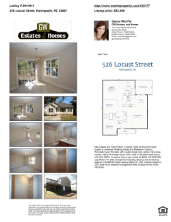
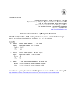


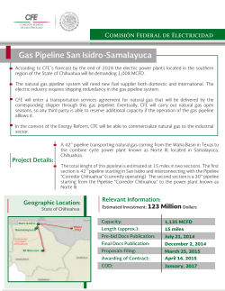
© Copyright 2026