1. No category

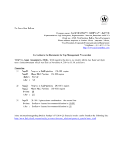
Use Cases for Linked Data Visualization Model
Jakub Klímek
Jiˇrí Helmich
Martin Neˇcaský
Czech Technical University in
Prague
Faculty of Information
Technology
Charles University in Prague
Faculty of Mathematics and
Physics
Charles University in Prague
Faculty of Mathematics and
Physics
[email protected]
[email protected]
[email protected]
ABSTRACT
There is a vast amount of Linked Data on the web spread
across a large number of datasets. One of the visions behind Linked Data is that the published data is conveniently
reusable by others. This, however, depends on many details
such as conformance of the data with commonly used vocabularies and adherence to best practices for data modeling.
Therefore, when an expert wants to reuse existing datasets,
he still needs to analyze them to discover how the data is
modeled and what it actually contains. This may include
analysis of what entities are there, how are they linked to
other entities, which properties from which vocabularies are
used, etc. What is missing is a convenient and fast way of
seeing what could be usable in the chosen unknown dataset
without reading through its RDF serialization. In this paper
we describe use cases based on this problem and their realization using our Linked Data Visualization Model (LDVM)
and its new implementation. LDVM is a formal base that
exploits the Linked Data principles to ensure interoperability
and compatibility of compliant analytic and visualization
components. We demonstrate the use cases on examples
from the Czech Linked Open Data cloud.
Categories and Subject Descriptors
H.5.2 [User interfaces]: GUIs, Interaction styles; H.3.5
[Online Information Services]: Data sharing; H.3.5 [Online
Information Services]: Web-based services
Keywords
Linked Data, RDF, visualization, discovery
1.
INTRODUCTION
A vast amount of data represented in a form of Linked
Open Data (LOD) is now available on the Web. Therefore,
the focus of Linked Data experts now starts to shift from
the creation of LOD datasets to their consumption and several new problems arise. Consider a Linked Data expert
working for a modern company who has a task of finding
suitable datasets in the LOD Cloud1 that would enhance
the company’s internal data. As of today, he can search
for the datasets in http://datahub.io, which is a CKAN2
1
2
http://lod-cloud.net/
http://ckan.org/
Copyright is held by the author/owner(s).
WWW2015 Workshop: Linked Data on the Web (LDOW2015).
catalog instance, which provides full–text search and keyword and faceted browsing of the textual metadata of the
datasets. To be able to decide whether a given dataset is
Elections
results
Budgets
Demogra
phy
LAU
regions
Exchange
rates
NUTS
codes
Czech
Ministry of
Finance
data
Contracts,
Invoices,
Payments
TED
Public
Contracts
Geocoordi
nates
COI.CZ
Governmental
Business-entities
Geographical
Statistical
RUIAN
ARES
Business
Entities
Research
projects
Czech
Business
Entity IDs
Czech
Public
Contracts
Institution
s of public
power
(OVM)
Czech
Social
Security
Administr
ation
CPV 2008
Consolida
ted Law
OVM
Agendas
Court
decisions
Figure 1: The 2015 Czech Linked Open Data Cloud
valuable for his use case or not, the expert needs to find out
whether it contains the expected entities and their properties. In addition, the entities and properties can be present
in the dataset, but they may be described using a different vocabulary than expected. A good documentation of
datasets is rare, therefore, the expert needs to go through
the dataset manually, either by loading it to his triplestore
and examining it using SPARQL queries or by looking at the
RDF serialization in a text editor. Only recently some other
technical approaches started to emerge such as LODeX [2]
that shows some statistics about the number of RDF triples,
classes, etc. and tries to extract the data schema from a
SPARQL endpoint. However, what the expert would really
need is a simple process where he would provide the data
and see whether the entities he expects, and maybe even
some others he does not expect, can be found in the given
dataset, and see them immediately. In this paper, we will
focus on this part of dataset consumption. Now let us assume
that the expert found a suitable dataset such as a list of all
cities and their geocoordinates and saw its map visualization.
This data could enhance his closed enterprise linked data
containing a list of the company’s offices. It would then be
useful for the expert if he could just include the appropriate
links from his dataset to the discovered one and see his offices
on a map in a generic visualization. It would be even better
if he could then refine this visualization instead of creating
another one from scratch.
In this paper we define the use cases which have the potential to help Linked Data experts in their work. Then
we briefly describe our Linked Data Visualization Model
(LDVM) [4] and show its new implementation, using which
we demonstrate that the use cases can be executed, which is
the main contribution of this paper. We will demonstrate our
approach using the datasets we prepare in our OpenData.cz
initiative, which can be seen in Figure 1, namely Institutions
of Public Power (OVM3 ) and registry of land identification,
addresses and properties of the Czech Republic (RUIAN4 ).
This paper is structured as follows. In Section 2 we define
the use cases we want to support by our approach. In Section 3 we briefly describe the principles and basic concepts of
LDVM. In Section 4 we introduce our new proof–of–concept
LDVM implementation and describe its components and relation to LDVM. In Section 5 we show a sample visualization
pipeline. In Section 6 we show how we use our implementation to support the defined use cases. In Section 7 we survey
related work and in Section 8 we conclude.
2.
MOTIVATING USE CASES
In this section we motivate our work using a series of use
cases with which we aim at helping Linked Data experts in
various stages of their work.
2.1
What Can I See in the Given Data
The first use case is to show possible visualizations of data
in a given dataset. The dataset must be given in an easy
way - using either a link to an RDF dump or using direct
RDF file upload, or using a link to a SPARQL endpoint that
contains the data. The result should be a list of possible
visualizations that could be meaningful for the dataset. When
the user clicks on a possible visualization, he should see his
data visualized by the selected technique, e.g. on a map,
using a hierarchy visualizer, etc. This use case has several
motivations. Firstly, one should be able to quickly sample a
previously unknown dataset that may be potentially useful
based on its textual description such as the one on http:
//datahub.io. Another motivation for this use case is the
need to be able to quickly and easily show someone what can
be done with his data in RDF. In addition, this use case can
help Linked Data experts even during the process of Linked
Data creation which usually happens in iterations. In the first
iteration of creating Linked Data an expert usually writes
a transformation of some basic information about entities
in the source data such as their names and types. Then he
reviews the created RDF data, selects another portion of
the source data, amends his transformation, executes it and
again observes the resulting, more detailed RDF data. He
repeats this process until all of the source data, or at least the
desired parts, is transformed to RDF. The iterations can be
3
4
http://datahub.io/dataset/cz-ovm
http://datahub.io/dataset/cz-ruian
fast, when the expert knows the source data and the desired
RDF form well, or they can be slow, when for example the
expert shows the result of each iteration to a customer and
discusses what part of the source data is he going to transform
next. Either way, it would be better to have a visualization
accompanying the data in each iteration, which would show
how the data gets better and more detailed. Also, trying
to visualize the resulting data provides additional means of
validation of the transformation, e.g. when it is entities on
a map, it is always better to see the result on a map than
just an RDF text file. On the other hand, the visualization
method needs to be quick and easy and not custom made
for the data, because the data between iterations is only
temporary as it lasts only until it gets improved in the next
iteration. However, this is made possible by the Linked
Data vocabulary reuse principle, all we need is a library of
components supporting standard vocabularies and usage of
the vocabularies in the data, which is a well known best
practice. Finally, when developing advanced visualizations,
the designer can start with the automatically offered one and
refine it instead of starting from scratch.
An example of this use case is that when a dataset containing a hierarchy is provided, then a visualization using a
hierarchy visualizer should be offered and it should display
some meaningful data from the source dataset. To be specific, we will show this use case on a dataset that contains a
hierarchy or regional units ranging from individual address
points to the whole country.
2.2
What Can I Combine My Data With To
See More
The second use case is to show which additional visualizations of the input data can be used when the data is simply
linked to another dataset. One motivation of this use case is
to visually prove the value of linking by showing the additional visualization options gained by it. Another motivation
is the expert in a modern company that has its internal
linked data and wants to see the improvement gained by
linking it to the public LOD cloud. For this use case the user
should be able to provide his data easily as in the previous
use case. This time he is interested in seeing which additional
visualizations of his data he can use when he linked his data
to another dataset. The result should again be a list of possible visualizations which, however, use not only the input
dataset, but also some other to achieve a better visualization.
For example, a dataset with addresses of public institutions,
linked to a geocoded dataset of all addresses yields a map
visualization with no additional effort.
2.3
What Data Can I Visualize Like This
The third use case is a reverse one compared to the previous two. It is to show datasets or their combinations which
can be visualized using a selected visualizer. The motivation
for this use case is that the user sees a visualization that he
likes and he wants to prepare his data so that it is compatible with the visualization. For that he wants to see which
other datasets possibly combined with some transformations
use this visualization. For this use case the user selects a
visualization and he should get a list of data sets possibly
with transformations which can be visualized by the selected
visualizer. For example, the user selects a map visualizer
and he should see that a dataset with a list of cities can be
visualized this way.
3.
LINKED DATA VISUALIZATION MODEL
To realize the use cases defined in the previous section
we will use a new implementation of our Linked Data Visualization Model (LDVM), which we defined and refined in
our previous work [4, 6, 8]. It is an abstract visualization
process customized for the specifics of Linked Data. In short,
LDVM allows users to create data visualization pipelines that
consist of four stages: Source Data, Analytical Abstraction,
Visualization Abstraction and View. The aim of LDVM is
to provide means of creating reusable components at each
stage that can be put together to create a pipeline even
by non-expert users who do not know RDF. The idea is to
let expert users to create the components by configuring
generic ones with proper SPARQL queries and vocabulary
transformations. In addition, the components are configured
in a way that allows the LDVM implementation to automatically check whether two components are compatible or not.
If two components are compatible, then the output of one
can be connected to the input of the other in a meaningful
way. With these components and the compatibility checking
mechanism in place, the visualization pipelines can then be
created by non-expert users.
3.1
Model Components
There are four stages of the visualization model populated
by LDVM components. Source Data stage allows a user
to define a custom transformation to prepare an arbitrary
dataset for further stages, which require their input to be
RDF. In this paper we only consider RDF data sources such
as RDF files or SPARQL endpoints, e.g. DBPedia. The
LDVM components at this stage are called data sources.
The Analytical Abstraction stage enables the user to specify
analytical operators that extract data to be processed from
one or more data sources and then transform it to create
the desired analysis. The transformation can also compute
additional characteristics like aggregations. For example, we
can query for resources of type dbpedia-owl:City and then
compute the number of cities in individual countries. The
LDVM components at this stage are called analyzers. In the
Visualization Abstraction stage of LDVM we need to prepare
the data to be compatible with the desired visualization
technique. We could have prepared the analytical abstraction
in a way that is directly compatible with a visualizer. In
that case, this step can be skipped. However, the typical
use case for Visualization Abstraction is to facilitate reuse
of existing analyzers and existing visualizers that work with
similar data, only in different formats. For that we need to
use a LDVM transformer. In View stage, data is passed to
a visualizer, which creates a user-friendly visualization. The
components, when connected together, create a analytic and
visualization pipeline which, when executed, takes data from
a source and transforms it to produce a visualization at the
end. Not every component can produce meaningful results
from any input. Typically, each component is designed for
a specific purpose, e.g. visualizing map data, and therefore
it does not work with other data. To create a meaningful
pipeline, we need compatible components.
3.2
Component Compatibility
Now that we described the four basic types of LDVM
components, let us take a look at the notion of their compatibility, which is the key feature of LDVM. We want to use the
checking of component compatibility in design time to rule
out component combinations that do not make any sense
and to help the users to use the right components before
they actually run the pipeline. Therefore, we need a way to
check the compatibility without the actual data.
Each LDVM component has a set of features, where each
feature represents a part of the expected component functionality. A component feature can be either mandatory or
optional. For example, a visualizer that displays points and
their descriptions on a map can have 2 features. One feature
represents the ability to display the points on a map. This
one will be mandatory, because without the points, the whole
visualization lacks purpose. The second feature will represent
the ability to display a description for each point on the map.
It will be optional, because when there is no data for the
description, the visualization still makes sense - there are
still points on a map. Whether a component feature can be
used or not depends on whether there is the data needed for
it on the input. Therefore, each feature is described by a set
of input descriptors. An input descriptor describes what is
expected on the inputs of the component. In this paper we
use a set of SPARQL queries for the descriptor. We could
also consider other forms of descriptors, but that is not in
the scope of this paper. A descriptor is applied to certain
inputs of its component.
In order to evaluate the descriptors in design time, we
require that each LDVM component that produces data (data
source, analyzer, transformer) also provides a sample of the
resulting data, which is called an output data sample. For the
data sample to be useful, it should be as small as possible,
so that the input descriptors of other components execute as
fast as possible on this sample. Also, it should contain the
maximum amount of classes and properties whose instances
can be produced by the component, making it as descriptive
as possible. For example, when an analyzer transforms data
about cities and their population, its output data sample will
contain a representation of one city with all the properties
that the component can possibly produce. Note that, e.g.
for data sources, it is possible to implement the evaluation
of descriptors over the output data sample as evaluation
directly on the represented SPARQL endpoint. For other
components, fast evaluation can be achieved by using a static
data sample.
We say that a feature of a component in a pipeline is
usable when all queries in all descriptors are evaluated true
on their respective inputs. A component is compatible with
the mapping of outputs of other components to its inputs
when all its mandatory features are usable. The usability of
optional features can be further used to evaluate the expected
quality of the output of the component. For simplicity, we
do not elaborate on the output quality in this paper. The
described mechanism of component compatibility can be used
in design time for checking of validity of the visualization
pipeline. It can also be used for suggestions of components
that can be connected to a given component output. In
addition, it can be used in run time for verification of the
compatibility using the actual data that is passed through
the pipeline. Finally, this concept can be also used for
periodic checking of data source content, e.g. whether the
data has changed its structure and therefore became unusable
or requires pipeline change. For a detailed description and
thorough examples of compatibility checking on real world
data see our previous paper [8].
Figure 2: LDVM Vocabulary
4.
ARCHITECTURE OF THE NEW LDVM
IMPLEMENTATION
In our previous LDVM implementation version Payola [7]
we had the following workflow. First, the pipeline designer
registered the data sources he was planning to use, if they
were not already registered. Then he started to create an
analysis by selecting data sources and then added analyzers
and transformers to the analytic pipeline. Then the pipeline
was executed and when done, the pipeline designer selected
an appropriate visualizer. There were no hints of which
visualizer is compatible with the result of the analysis and this
workflow contained unnecessary steps. The pipeline and its
components existed only inside Payola with no means of their
creation and management from the outside. Nevertheless it
demonstrated some advantages of our approach. It showed
that pipelines created by expert users can be reused by lay
users and the technical details can be hidden from them.
It also showed that results of one analysis can be used by
various visualizers and also it showed that one analysis can
run on various data sources.
In our new implementation of LDVM we aim for having
individual components running as independent web services
that accept configuration and exchange information needed
to get the input data and to store the output data. Also
we aim for easy configuration of components as well as easy
configuration of the whole pipeline. In accordance with the
Linked Data principles, we now use RDF as the format for
storage and exchange of configuration so that any code that
works with RDF can create, maintain and use LDVM components both individually and in a pipeline. For this purpose
we have devised a vocabulary for LDVM. In Figure 2 there is
a UML class diagram depicting the structure of the LDVM
vocabulary. Boxes represent classes, edges represent object
properties (links) and properties listed inside of the class
boxes represent data properties. The architecture of our new
implementation corresponds to the vocabulary. The data
entities correspond to software components and their configuration. We chose the ldvm5 prefix for the vocabulary. The
vocabulary and examples are developed on GitHub6 . Let us
now briefly go through the individual parts of the vocabulary,
which correspond to parts of the LDVM implementation
architecture.
4.1
Templates and Instances
In Figure 2 there are blue and green (dashed) classes.
The blue classes belong to template level of the vocabulary
and green classes belong to the instance level. These two
levels directly correspond to two main parts of the LDVM
implementation. At the template level we register LDVM
components as abstract entities described by their inputs,
outputs and default configuration. At the instance level we
have a pipeline consisting of interconnected specific instances
of components and their configurations. The easiest way to
imagine the division is to imagine a pipeline editor with a
toolbox. In the toolbox, there are LDVM component templates and when a designer wants to use a LDVM component
in a pipeline, he drags it onto the editor canvas, creating an
instance. There can be multiple instances of the same LDVM
5
6
http://linked.opendata.cz/ontology/ldvm/
https://github.com/payola/ldvm
component template in a single pipeline, each with a different
configuration that overrides the default one. The template
holds the input descriptors and output data samples which
are used for the compatibility checking together with the
instance input and output mappings. Each instance is connected to its corresponding template using the instanceOf
property.
4.2
Component Types
There are four basic component types as described in
Section 3.1 - data sources, analyzers, transformers and visualizers. They have their representation on both the template
level - descendants of the ComponentTemplate class - and instance levels - descendants of the ComponentInstance class.
From the implementation point of view, transformers are just
analyzers with one input and one output, so the difference
is purely semantic. This is why transformers are subclass of
analyzers.
4.3
Data Ports
Components have input and output data ports. On the
template level we distinguish the inputs and outputs of a
component. To InputDataPortTemplate the input descriptors of features can be applied. OutputDataPortTemplate
has the outputDataSample links to the output data samples.
Both are subclasses of DataPortTemplate. The data ports
are mapped to each other - output of one component to
input of another - as instances of DataPortInstance using
the boundTo property. This data port instance mapping
forms the actual visualization pipeline which can be then executed. Because data ports are not LDVM components, their
instances are connected to their templates using a separate
property dataPortInstanceOf.
4.4
Features and Descriptors
On the template level, features and descriptors (see Section 3.2) of components are represented. Each component
template can have multiple features connected using the
feature property. The features themselves - instances of
either the MandatoryFeature class or the OptionalFeature
class - can be described using standard Linked Data techniques and vocabularies such as dcterms and skos. Each
feature can have descriptors, instances of Descriptor connected using the descriptor property. The descriptors have
their actual SPARQL queries as literals connected using the
query property. In addition, the input data port templates
to which the particular descriptor is applied are denoted
using the appliesTo property.
4.5
Configuration
Now that we have the LDVM components, we need to
represent their configuration. On the template level, components have their default configuration connected using
the componentConfigurationTemplate property. On the
instance level, components point to their configuration using
the componentConfigurationInstance property when it is
different from the default one. The configuration itself is the
same whether it is on the template level or the instance level
and therefore we do not distinguish the levels here and we
only have one class ComponentConfiguration.
The structure of the configuration of a LDVM component
is completely dependent on what the component needs to
function. It is also RDF data and it can use various vocabu-
laries. It can be even linked to other datasets according to
the Linked Data principles. Therefore it is not a trivial task
to determine the boundaries of the configuration data in the
RDF data graph in general. On the other hand, each component knows precisely what is expected in its configuration
and in what format. This is why we need each component
to provide a SPARQL query that can be used to obtain
its configuration data so that the LDVM implementation
can extract it. That SPARQL query is connected to every
configuration using the mandatory configurationSPARQL
property.
4.6
Pipeline
Finally, the pipeline itself is represented by the Pipeline
class instance. It links to all the instances of LDVM components used in the pipeline. Another feature supporting collaboration of expert and non-expert users is pipeline nesting.
An expert can create a pipeline that is potentially complex in
number of components, their configuration and binding, but
could be reused in other pipelines as a black box data source,
analyzer or transformer. As this feature is not important in
this paper, we do not further describe it. It is sufficient to say
that the nestedPipeline and nestedBoundTo properties of
LDVM serve this purpose.
4.7
Component Compatibility Checking
The component compatibility checks (see Section 3.2) are
exploited in various places. The checks can happen during
run time when the actual data passed between components
is verified as it is passed along the pipeline. They can also
happen in scheduled intervals when existing pipelines are
re-checked to determine possible changes in data sources that
can cause pipelines to stop being executable. This can be
easily used for verification of datasets that change frequently.
Another usage of the checks is during design of a pipeline in a
future pipeline editor, which is not implemented yet, when a
user wants to connect two components in a pipeline. However,
the most valuable usage of component compatibility checking
is in the pipeline discovery algorithm.
4.8
Pipeline Discovery Algorithm
The pipeline discovery algorithm is used to generate all
possible pipelines based on a set of datasets and is therefore
the core functionality for this paper and the use cases it
demonstrates. It is inspired by the classical Breadth-first
search (BFS) algorithm where, simply put, an edge between
two nodes representing LDVM components in a pipeline exists if and only if the descriptor of the second one matches
the output data sample of the first one. The edge then represents the possibility to pass data from the output of the first
component to the input of the second component. The algorithm works in iterations and builds up pipeline fragments
in all compatible combinations. We will demonstrate it on
an example of two data sources (RUIAN, Institutions), a
RUIAN geocoder analyzer, which takes two inputs, a Towns
extractor, and a Google Maps visualizer.
It starts with the inputs of all available LDVM components
(analyzers, transformers, visualizers) checking selected data
sources, which form trivial, one member pipeline fragments.
In Figure 3 we can see the trivial fragments in the top
right part. In the first step every available component is
checked with each selected data source. When a component’s
input is compatible with the output of the last component
ented from leaves to root where leaves are data sources and
the root is the visualizer. Of course the complexity of this
algorithm raises with the number of components and data
sources to check. On the other hand the compatibility checks
greatly reduce the number of possibilities and leave only the
compatible ones. A more rigorous measurements of time
consumed are part of our future work.
4.9
Figure 3: Pipeline discovery iteration 1
of a pipeline fragment (output of a data source in the first
iteration), it is connected. A successful check is denoted by
a green arrow and a unsuccessful one with a red arrow.
When all of the components inputs are connected, the component is added to the pipeline fragment and this fragment
gets checked again by all LDVM component inputs in the
next iteration. This is visible in Figure 4 – a pipeline fragments from iteration 1 ending with the RUIAN geocoder are
not checked until both inputs of the geocoder are connected,
which happens in iteration 2 and 3. When the algorithm
reaches a visualizer and binds all of its inputs, the pipeline
fragment leading to this visualizer is saved as a possible
pipeline. This happens in Figure 3 with the 2 member
pipeline and in Figure 4 iterations 3 and 4. When there are
no new pipeline fragments to consider in the next algorithm
iteration, we have generated all possible pipelines and the
algorithm ends. In the example we generated 3 pipelines.
Note that the generated pipelines are in a form of trees ori-
Component implementations
Note that we have not talked about the actual LDVM
component implementations yet, only templates, which are
abstract descriptions and default configurations, and instance,
which are representations in a pipeline with inputs and outputs bound to other components. Our vision is to have
LDVM component implementations as standalone web services configurable by RDF, reusable among LDVM instances
and other applications. They would live separately from our
LDVM implementation instance, which would then serve
only as a pipeline editor, catalog and launcher (see Figure 6).
The components would register to the LDVM instance with
access data and a link to LDVM templates that can be
processed using this component implementation. The RDF
Figure 6: LDVM implementation and LDVM components
configuration sent to the component implementation would
contain the actual component instance configuration together
with access information for getting input data, storing output data and a callback URL for sending execution result
information. The execution result information would include
the status (success, failure) and optionally logs to be displayed to the pipeline user. However, the complete freedom
of the components is not a trivial development task, so it
still remains a part of our future work. Now, the actual
component implementations we use run on the same machine
as the LDVM implementation and we have a hard coded list
of which components can process which LDVM component
templates. Nevertheless, this implementation limitation does
not affect the use cases we show in this paper.
5.
Figure 4: Pipeline discovery - more iterations
LDVM PIPELINE EXAMPLE
Let us now briefly demonstrate how a simple LDVM
pipeline looks like from the data point of view. See Figure 5. Again, we will have blue for template level and green
Figure 5: Sample LDVM Pipeline
(dashed) for instance level. The instance level is simpler,
let us start with it. On the bottom we have a pipeline,
which points to LDVM component instances that belong to
the pipeline via the ldvm:member property. It is a simple
pipeline consisting of one data source, one analyzer and a
visualizer. The data source instance is configured to access
our RUIAN SPARQL endpoint and it is an instance of a
generic SPARQL endpoint data source template. The analyzer instance extracts information about Czech towns from
the data source, which contains far more information. The
descriptor of the analyzer’s feature Input contains Towns is
a SPARQL ASK query which checks for presence of a data
source with towns information and is applied to the input
data port template of the analyzer. The output data port
template of the analyzer has a link to an output data sample,
which is a Turtle file containing data about one Czech town
as a sample. This brings us to the Google Maps visualizer,
which only has input data port template with one feature
and a descriptor checking for presence of geocoordinates in
its input data. Note that the data port binding is done on
the instance level, which is what will be seen and edited in a
pipeline editor. On the other hand, features, descriptors and
output data samples are all on the template level. Because
RUIAN includes geocoordinates for each entity, the resulting
visualization shows towns in the Czech Republic on a map.
6.
REALIZATION OF USE CASES
In our new proof–of–concept implementation of LDVM
(LDVMi) we aim at a more straight forward workflow utilizing the compatibility checking feature of LDVM. The goal
is to provide the user with some kind of a meaningful visual representation of his data as easily as possible. This
means that the user specifies the location of his data and
that should be all that is needed to show some initial visualizations. This is achieved by our compatibility checking
mechanism (see Section 3.2) using which we generate all possible pipelines that can be created using the data sources and
LDVM components registered in the used LDVM instance.
We are still in early stages of the new implementation, it
runs at http://ldvm.opendata.cz and all the mentioned
LDVM components should be loaded there. The use cases
from this section should be executable there and anyone can
experiment with any SPARQL endpoint or RDF data that
is compatible with the loaded components.
Figure 7: Endpoint selection
6.1
What Can I See in the Given Data
In this use case we are in the role of a Linked Data expert
that has a link to a dataset and wants to quickly see what
can be seen in it. The actual offered visualizations depend
solely on the set of analyzers, transformers and visualizers
present in the LDVM instance. We assume that the expert
has his LDVM instance populated with components that he
plans to use and he checks a potentially useful dataset he
has a link to. For the realization of this use case we will use
the RUIAN dataset. It contains a lot of data among which
is a hierarchy of regional units ranging from address points
to the whole country modeled using SKOS. We have a link
to the dataset in a SPARQL endpoint, so we point to it (see
Figure 7). Next, we see the list of possible pipelines based
on the evaluation of compatibility with the endpoint, see
Figure 8. We can see that there are 3 pipelines. We can
also see their data sources, their visualizer, and in between
Figure 10: File upload
Figure 8: Possible pipelines list
the number of analyzers the pipeline contains. The first two
end with a Google Map visualizer – the dataset contains
geocodes for all objects – and the third one with a TreeMap
hierarchy visualization, which means that a hierarchy was
found in our dataset and it can be visualized. We select
the third pipeline and we see the hierarchy as in Figure 9.
This proves that using a LDVM instance populated with
of Public Power from DataHub.io. This could also be an
internal dataset of a company. Note that we will also add
the schema of the data for better filtering in the visualizer,
which would, however, typically be in the second iteration
after we found out that without it, we cannot filter properly
in the visualizer, but we would still see the towns on the map.
The dump and schema are in TriG serialization, which is not
yet supported, however it is easy to convert it to Turtle. We
upload the schema7 , the links8 to the RUIAN dataset and
the data in Turtle9 as in Figure 10. After the file upload is
finished, we see the possible pipelines as in Figure 11. Note
Figure 11: Possible pipelines for dataset combination
Figure 9: Treemap visualization of a simple hierarchy
a set of LDVM components, we can easily check whether
a given dataset contains usable data and see some initial
results quickly. This is thanks to the static data samples
and SPARQL ASK based descriptors. As part of our future
work we will do rigorous measurements to see the response
times according to number of components and number and
complexity of descriptors.
6.2
What Can I Combine My Data With To
See More
We assume that we have the RUIAN data source and Maps
visualizer registered in our LDVM instance. In addition, we
will have a RUIAN Towns geocoder analyzer registered, which
takes a list of towns from RUIAN (reference dataset) on one
input and the dataset linked to RUIAN (linked dataset) on
the other input. It outputs the linked dataset enhanced with
GPS geocoordinates of the entities from the reference dataset.
For this use case, we will use our dataset of Institutions
that this pipeline discovery is the same as in the example in
4.8 with one difference. There, the algorithm searched for all
pipelines that could be created from the two datasets, which
included a direct visualization of RUIAN on a map. Here,
the discovery algorithm does not return this pipeline because
it searches for pipelines that visualize the linked dataset in
combination with other data sources. Therefore, we have two
possibilities of how to see our newly linked dataset on a map.
One is applying the RUIAN Towns geocoder to the linked
dataset and takes the whole RUIAN data source as the other
input. This one, while theoretically possible, is not usable in
our current implementation because the whole RUIAN data
source is large (600M triples) and contains tens of thousands
of entities of various types. This is why we will choose the
other possible pipeline, which, in addition, runs the RUIAN
data through RUIAN Towns extractor analyzer, which filters
out data about other RUIAN entities. The chosen pipeline
can be seen in Figure 12. All that is left is to evaluate the
pipeline (press the Run button) and display the resulting
visualization that can be seen in Figure 13. The filtering of
7
8
http://opendata.cz/ldvm/ovm-vocab.ttl
https://raw.githubusercontent.com/payola/ldvm/master/rdf/
examples/ovm-obce-links.ttl
9
http://opendata.cz/ldvm/ovm.ttl
our LDVM instance. In this list, we will choose the desired
visualizer such as the Google Map visualizer. There we click
Figure 14: All pipelines using this visualizer
Figure 12: The chosen pipeline combining datasets
displayed institution of public power is possible thanks to
the schema that we included in the beginning. Note that the
compatibility checks so far have a form of a query that checks
for a presence of certain class and property instances in a
dataset. E.g. in this use case, we determine the presence of
links to RUIAN by presence of properties which we created
for linking to RUIAN objects in the RUIAN vocabulary and
we rely on creators of other datasets that they will use these
properties when linking their data to RUIAN. What we do
not check for at this time is whether the links in one dataset
lead to existing or valid objects in the second dataset, because
that would require non–trivial querying.
Figure 13: Maps visualization of linked dataset with
filtering
This means that if someone connected a dataset of German towns represented using our RUIAN vocabulary to the
RUIAN geocoder analyzer together with the Czech Institutions of Public Power, he would get a compatible pipeline.
However, this pipeline would not produce any usable data
on evaluation as the two input datasets simply do not have
matching contents. We will look into possibilities of checking
for these situations in our future work.
6.3
the list pipelines using this visualizer button (see Figure 14)
and we see the list of pipelines that contain it. This tells
us the data sources and their possible transformations using
analyzers and transformers that result in data that can be
visualized by the chosen visualizer.
7.
RELATED WORK
More and more projects are focused on analyzing, exploring and visualizing Linked Data. For a more complete survey
of various Linked Data visualization tools see our previous
paper [8]. Here, we will focus on the most recent approaches.
With the LDVM vocabulary and our new implementation
we aim at an open web-services like environment that is
independent of the specific implementation of the LDVM
components. This of course requires proper definition of
interfaces and the LDVM vocabulary is the base for that.
However, the other approaches so far usually aim at a closed
browser environment. Those are similar to our Payola [7]
in their ability to analyze and visualize parts of the Linked
Data cloud. They do not provide configuration and description using a reusable vocabulary and they do not aim at
a more open environment with their implementation that
would allow other applications to reuse their parts. Recent
approaches include Hide the stack [5], where the authors
describe a browser meant for end-users which is based on
templates based on SPARQL queries. Also recent is LDVizWiz [1], which is a very LDVM-like approach to detecting
categories of data in SPARQL endpoints and extracting basic
information about entities in those categories. An lightweight
application of LDVM in enterprise is described in LinDa [10].
Yet another similar approach that analyzes SPARQL endpoints to generate faceted browsers is rdf:SynopsViz [3]. In
[2] the authors use their LODeX tool to summarize LOD
datasets according to the vocabularies used.
The most relevant related work to the specific topic of a
vocabulary supporting Linked Data visualization is Fresnel
- Display Vocabulary for RDF [9]. Fresnel specifies how a
resource should be visually represented by Fresnel-compliant
tools like LENA 10 and Longwell 11 . Therefore, Fresnel vocabulary could be perceived as a vocabulary for describing
LDVM visualization abstraction. This is partly because the
vocabulary was created before the Linked Data era and therefore focuses on visualizing RDF data without considering
vocabularies and multiple sources.
What Data Can I Visualize Like This
In this use case we will find datasets that are visualizable
by a specific visualizer. It is in fact a simple filter of all
known possible pipelines that contain this visualizer. For
this use case we go to the list of available components in
8.
10
11
CONCLUSIONS AND FUTURE WORK
https://code.google.com/p/lena/
http://simile.mit.edu/issues/browse/LONGWELL
In this paper we defined use cases that aid Linked Data
experts in various stages of their work and showed how we
can realize them using our implementation of the Linked
Data Visualization Model (LDVM). The first use case was
to easily show contents of a given dataset using LDVM
components and mainly visualizers. The second use case was
to show for a given dataset with which other known datasets
it can be combined to achieve a visualization. The third use
case was to show which known datasets can be visualized
using a selected visualizer so that the expert can adjust his
data accordingly. Then we briefly described LDVM and its
vocabulary and implementation and our vision of LDVM
components as independent web services. Finally, we showed
that using the LDVM implementation populated by LDVM
components we are able to execute the defined use cases.
During our work we have identified multiple directions
we should investigate further. When we evolve our LDVM
implementation into a distributed system with components
as individual web services, many new opportunities will
arise. We could be able to do load balancing, where we will
have multiple implementations running on multiple machines
able to process the same LDVM template and its instances.
Also, the SPARQL implementations, while identical in principle, can be differentiated using various properties. One of
those properties can be the actual SPARQL implementation
used as, from our experience, every implementation supports
SPARQL in a slightly different way or supports a slightly
different subset of it. Also, the same SPARQL query can run
substantially faster on one implementation and substantially
slower on another one, etc. Another direction to investigate
further is towards Linked Data Exploration – a process of
searching the Linked Data Cloud for datasets that contain
data that we can reuse. Our approach so far requires selecting
the dataset to investigate. However, that alone can be a non–
trivial effort and using Linked Data Exploration we could
identify the datasets for LDVM processing based on some
form of user requirements. Our closest goal of course is to
make our new LDVM implementation more user friendly and
to develop a more presentable library of visualizers, analyzers
and transformers.
9.
ACKNOWLEDGMENTS
This work was partially supported by a grant from the European Union’s 7th Framework Programme number 611358
provided for the project COMSODE.
10.
REFERENCES
[1] G. A. Atemezing and R. Troncy. Towards a
Linked-Data based Visualization Wizard. In O. Hartig,
A. Hogan, and J. Sequeda, editors, Proceedings of the
5th International Workshop on Consuming Linked Data
(COLD 2014) co-located with the 13th International
Semantic Web Conference (ISWC 2014), Riva del
Garda, Italy, October 20, 2014., volume 1264 of CEUR
Workshop Proceedings. CEUR-WS.org, 2014.
[2] F. Benedetti, S. Bergamaschi, and L. Po. Online Index
Extraction from Linked Open Data Sources. In A. L.
Gentile, Z. Zhang, C. d’Amato, and H. Paulheim,
editors, Proceedings of the 2nd International Workshop
on Linked Data for Information Extraction (LD4IE),
number 1267 in CEUR Workshop Proceedings, pages
9–20, Aachen, 2014.
[3] N. Bikakis, M. Skourla, and G. Papastefanatos.
rdf:SynopsViz – A Framework for Hierarchical Linked
Data Visual Exploration and Analysis. In V. Presutti,
E. Blomqvist, R. Troncy, H. Sack, I. Papadakis, and
A. Tordai, editors, The Semantic Web: ESWC 2014
Satellite Events, Lecture Notes in Computer Science,
pages 292–297. Springer International Publishing, 2014.
[4] J. M. Brunetti, S. Auer, R. Garc´ıa, J. Kl´ımek, and
M. Neˇcask´
y. Formal Linked Data Visualization Model.
In Proceedings of the 15th International Conference on
Information Integration and Web-based Applications &
Services (IIWAS’13), pages 309–318, 2013.
[5] A.-S. Dadzie, M. Rowe, and D. Petrelli. Hide the Stack:
Toward Usable Linked Data. In G. Antoniou,
M. Grobelnik, E. Simperl, B. Parsia, D. Plexousakis,
P. De Leenheer, and J. Pan, editors, The Semantic
Web: Research and Applications, volume 6643 of
Lecture Notes in Computer Science, pages 93–107.
Springer Berlin Heidelberg, 2011.
[6] J. Helmich, J. Kl´ımek, and M. Neˇcask´
y. Visualizing
RDF data cubes using the linked data visualization
model. In V. Presutti, E. Blomqvist, R. Troncy,
H. Sack, I. Papadakis, and A. Tordai, editors, The
Semantic Web: ESWC 2014 Satellite Events - ESWC
2014 Satellite Events, Anissaras, Crete, Greece, May
25-29, 2014, Revised Selected Papers, volume 8798 of
Lecture Notes in Computer Science, pages 368–373.
Springer, 2014.
[7] J. Kl´ımek, J. Helmich, and M. Neˇcask´
y. Payola:
Collaborative Linked Data Analysis and Visualization
Framework. In 10th Extended Semantic Web
Conference (ESWC 2013), pages 147–151. Springer,
2013.
y. Application of
[8] J. Kl´ımek, J. Helmich, and M. Neˇcask´
the Linked Data Visualization Model on Real World
Data from the Czech LOD Cloud. In C. Bizer,
T. Heath, S. Auer, and T. Berners-Lee, editors,
Proceedings of the Workshop on Linked Data on the
Web co-located with the 23rd International World Wide
Web Conference (WWW 2014), Seoul, Korea, April 8,
2014., volume 1184 of CEUR Workshop Proceedings.
CEUR-WS.org, 2014.
[9] E. Pietriga, C. Bizer, D. R. Karger, and R. Lee.
Fresnel: A Browser-Independent Presentation
Vocabulary for RDF. In I. F. Cruz, S. Decker,
D. Allemang, C. Preist, D. Schwabe, P. Mika,
M. Uschold, and L. Aroyo, editors, The Semantic Web ISWC 2006, 5th International Semantic Web
Conference, ISWC 2006, Athens, GA, USA, November
5-9, 2006, Proceedings, volume 4273 of Lecture Notes in
Computer Science, pages 158–171. Springer, 2006.
[10] K. Thellmann, F. Orlandi, and S. Auer. LinDA Visualising and Exploring Linked Data. In Proceedings
of the Posters and Demos Track of 10th International
Conference on Semantic Systems - SEMANTiCS2014,
Leipzig, Germany, 9 2014.