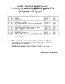
INSTITUTE OF PHYSICS PUBLISHING
JOURNAL OF OPTICS A: PURE AND APPLIED OPTICS
J. Opt. A: Pure Appl. Opt. 8 (2006) S518–S523
doi:10.1088/1464-4258/8/7/S33
Interference techniques in digital
holography
Myung K Kim, Lingfeng Yu and Christopher J Mann
Department of Physics, University of South Florida, Tampa, FL 33620, USA
E-mail: [email protected]
Received 17 November 2005, accepted for publication 23 February 2006
Published 8 June 2006
Online at stacks.iop.org/JOptA/8/S518
Abstract
Interference techniques in digital holography are discussed and experimental
results from each technique are presented. Numerical reconstruction
algorithms for digital holography are reviewed. The angular spectrum
method is seen to be particularly advantageous, with the ability to remove
noise and unwanted holographic terms. The dual wavelength optical
unwrapping technique offers an unambiguous method of removing 2π phase
discontinuity. Application of wavelength-scanning digital interference
holography is used to obtain tomographic images with synthesized short
coherence length.
Keywords: digital holography, interference imaging, phase contrast
microscopy, optical tomography
(Some figures in this article are in colour only in the electronic version)
1. Introduction
Digital holography has been experiencing rapid development
in recent years because of many technical advantages,
including a number of interference techniques that are
unavailable or difficult and cumbersome in conventional
holography. The principle of holography was first suggested
by Gabor in 1948, as a method of recording complete threedimensional information of an object wave [1]. With the
later invention of the laser and the introduction of the off-axis
technique in 1962 [2], holography quickly gained scientific
recognition. The advances in digital imaging and computation
technologies have now made it feasible and advantageous
to replace the photochemical processing of conventional
holography with CCD arrays and numerical computation.
A digital hologram is created by the interference between
a coherent object and reference beam, which is digitally
recorded by a CCD camera and processed by computational
methods to obtain the holographic images [3–5]. The digital
hologram contains not only amplitude information of the
object, but also phase [6, 7]. Moreover, the ability of the
CCD camera to quantify the recorded light gives rise to a
number of post-processing methods that can for instance be
used to calculate optical thickness or refractive index variations
of an object provided knowledge of one or the other is
available. Digital holography has been applied in diverse
1464-4258/06/070518+06$30.00
fields including metrology [8], deformation measurement [9],
vibrational analysis [10] and more recently biological
microscopy [11–14].
The applications to microscopy
are particularly advantageous.
Conventional bright-field
microscopes have difficulty in observing transparent samples
which exhibit little intensity contrast. The phase contrast
microscopy technique of Zernike and differential interference
contrast (DIC) microscopy of Nomarksi do not offer direct
quantitative evaluation of the phase information.
The
unavailability of this information in these techniques presents a
difficulty in observing and interpreting morphological changes
and properties of a sample.
Digital holography not only offers quantitative phase
information but high fidelity and high resolution images
with precision of optical thickness on the order of tens of
nanometres [15]. Another appealing aspect of the technique
is numerical focusing, emulating the focusing control of
conventional microscopes. In particular, the use of the angular
spectrum reconstruction algorithm provides a significant
advantage in focusing and reconstruction [16]. It has no
minimum distance requirement from the object to the hologram
plane and allows for flexible and effective filtering and control
of the zero order and spurious noise components from sources
such as stray reflections. A common presumption is that
coherent imaging suffers from the image degrading effect of
coherent noise; however, through careful control of the laser
© 2006 IOP Publishing Ltd Printed in the UK
S518
Interference techniques in digital holography
kx
k
kz
z
E0(x0,y0)
E(x,y)
Figure 2. Coordinate system for reconstruction of the hologram in
the angular spectrum method.
Figure 1. Digital holography experiments using transmission (a) and
reflective (b) geometries.
beam and other optical quality, remarkably clean images can
be obtained. This is especially true with phase imaging digital
holography because of its relative immunity to amplitude or
phase noise of the laser profile.
2. Numerical diffraction: theory
The digital holography experiments are performed in both
transmission and reflective geometries as depicted in figure 1.
The output from the laser, spatially filtered and collimated, is
split into an object and reference beam in an interferometer
based on the Mach–Zehnder configuration. The object
specimen, mounted on an x yz -translation stage, is placed at
a distance z from the hologram plane H , which is imaged
and magnified by the lens L1 and projected onto the CCD
array. The reference beam is similarly magnified by lens L2
and the interference between the object and reference beams
is recorded and stored onto a computer. Once the hologram
has been recorded, it remains to reconstruct the optical field by
computationally simulating diffraction using one of a number
of numerical methods.
2.1. Huygens convolution method
The convolution approach represents a computationally
heaviest form of holographic reconstruction with modest
degree of accuracy [17]. The reconstructed complex wavefield
E(x, y) is found by
ik
E(x, y; z) = −
E 0 (x0 , y0 )
2π
(1)
× exp ik (x − x0 )2 + (y − y0 )2 + z 2 dx0 d y0 .
This is a convolution:
E(x, y; z) = E 0 (x, y) ∗ SH (x, y, z)
= F−1 [F(E 0 ) · F(SH )]
(2)
where SH is the Huygens PSF
ik
SH (x, y, z) = −
exp ik x 2 + y 2 + z 2 .
2π z
of the images reconstructed by the convolution approach are
equal to that of the hologram. In order to achieve as high a
lateral resolution as possible, one keeps the object–hologram
distance as short as possible, but the discrete Fourier transform
necessitates a minimum distance such that
z min =
The whole process requires three Fourier transforms, which
are carried out using the FFT algorithm. The pixel sizes
(4)
where ax = n x x is the size of the hologram and n x
and x are the number and size of pixels. At too close a
distance, the spatial frequency of the hologram is too low and
aliasing occurs. Normally the object is placed just outside this
minimum distance.
2.2. Fresnel transform method
The Fresnel transformation [3] is the most commonly
used method in holographic reconstruction, because of the
computational efficiency. The approximation of a spherical
Huygens wavelet by a parabolic surface allows the calculation
of the diffraction integral using a single Fourier transform. The
PSF can be simplified by the Fresnel approximation as
S(x, y; z) = −
ik
k
exp ikz + i (x 2 + y 2 )
2π z
2z
and the reconstructed wavefield is
ik
ik 2
2
E(x, y; z) = −
exp ikz + (x + y )
2π z
2z
ik 2
×
E 0 (x0 , y0 ) exp
(x0 + y02 )
2z
ik
× exp − (x x0 + yy0 ) dx0 d y0
z
ik 2
2
= exp
(x + y ) F[E 0 · S].
2z
(5)
(6)
The resolution x of the reconstructed images determined
directly from the Fresnel diffraction formula will vary as a
function of the reconstruction distance z as
α =
(3)
ax2
,
nx λ
λz
N x0
(7)
where N is the number of pixels and x0 is the pixel width
of the CCD camera. As with the Huygens convolution method
there is a minimum z distance requirement set by equation (4).
S519
M K Kim et al
Figure 3. Numerical focusing in digital holography of an element of a USAF 1951 resolution target from a single hologram. Images are of a
30 × 30 µm2 area (360 × 360 pixels) with z scanned from 1 to 15 µm in steps of 2 µm.
Figure 4. Holography of a SKOV ovarian cancer cell. The image area is 60 × 60 (424 × 424 pixels) and the image is at z = 1.0 µm from the
hologram: (a) hologram; (b) angular spectrum; (c) amplitude and (d) phase images by the angular spectrum method; (e) unwrapped phase
image of (d); (f) amplitude and (g) phase images by the Huygens convolution method. (h) 3D perspective rendering of (e).
2.3. Angular spectrum method
The angular spectrum method [16] is seen to be fairly efficient
computationally but with the highest degree of accuracy.
Refering to figure 2, if E 0 (x0 , y0 ; 0) is the wavefield at plane
z = 0, the angular spectrum A(k x , k y ; 0) at this plane is
obtained by taking the Fourier transform:
A(k x , k y ; 0) =
E 0 (x0 , y0 ; 0)
× exp[−i(k x x0 + k y y0 )] dx0 d y0
(8)
where k x and k y are corresponding spatial frequencies of x and
y . Fourier-domain filtering can be applied to the spectrum to
block unwanted spectral terms in the hologram and select a
region of interest corresponding only to the object spectrum. A
modified wavefield E¯ 0 (x0 , y0 ; 0) can be written as the inverse
¯ x , k y ; 0),
Fourier transform of the filtered angular spectrum A(k
E¯ 0 (x0 , y0 ; 0) =
¯ x , k y ; 0) exp[i(k x x0 +k y y0 )] dk x dk y .
A(k
(9)
S520
The angular spectrum at plane
z, A(k x , k y ; z) is calculated
¯
from A(k x , k y ; 0), with k z = k 2 − k x2 − k 2y
¯ x , k y ; 0) exp[ik z z].
A(k x , k y ; z) = A(k
(10)
The reconstructed complex wavefield of any plane perpendicular to the propagating z axis is found by
E(x, y; z) =
A(k x , k y ; z) exp[i (k x x + k y y)] dk x dk y
= F−1 {filter[F{E 0 }] exp[ik z z]}.
(11)
Here ‘filter’ represents filtering in the spectral domain.
Two Fourier transforms are needed for the calculation in
comparison to the one needed by the Fresnel transform.
However, once the field is known at any one plane, only one
additional Fourier transform is needed to calculate the field at
different values of z . This method allows frequency-domain
spectrum filtering to be applied, which for example can be
used to block or remove the disturbance of the zero order and
twin image component. A significant advantage of the angular
spectrum is that there is no minimum z distance requirement.
Interference techniques in digital holography
Figure 5. Holography of an onion nucleus. The image area is
30 × 30 µm2 (436 × 436 pixels) and the image is at z = 22 µm from
the hologram: (a) hologram; (b) holographic amplitude and (c) phase
images; (d) unwrapped phase image; (e) 3D pseudo-colour rendering
of (d).
Figure 6. Holography of a living SKOV ovarian cancer cell. The
image area is 70 × 70 µm2 (448 × 448 pixels) and the image is at
z = 12 µm from the hologram: (a) hologram; (b) amplitude and
(c) phase images; (d) unwrapped phase image; (e) 3D perspective
rendering of (d).
2.4. Numerical focusing
The optical field can be calculated at any number of image
planes from a single hologram, emulating the mechanical
focusing control of a conventional microscope. To illustrate
this focusing ability we show a sequence of eight images in
figure 3 calculated in the range of z = 1–15 µm in steps of
2 µm. Each image is a 30 × 30 µm2 area of a resolution target.
As the focus is scanned, one observes the bars move into focus
as it passes through the various image planes.
3. Quantitative phase imaging
Figure 4 illustrates the implementation of the numerical
algorithms in the reconstruction of a SKOV3 ovarian cancer
cell. The area is 60 × 60 µm2 with 424 × 424 pixels. Figure 4(a)
is the holographic interference pattern recorded by the CCD
camera, and its Fourier transform in figure 4(b) is the angular
spectrum. It contains both the zero order and twin images,
as well as artifact due to stray interference components. The
virtual image component, the highlighted circular area, is
selected. A propagation phase factor (z = 1.0 µm) is
multiplied, and finally inverse-Fourier transformed to obtain
the amplitude image in figure 4(c) and the phase image in
figure 4(d). The physical thickness of the cell can be calculated
from
d = λ(ϕ/2π)/(n − n 0 )
(12)
where λ is the wavelength, ϕ is the phase step and (n − n 0 ) is
the index difference between the film and air. For example, the
layer of lamellipodia around the edge of the cell is found to be
about 110 nm, assuming n = 1.375 for the cell. The phase map
is rendered in pseudo-coloured 3D perspective in figure 4(h).
Especially notable in the phase map is the lack of the coherent
noise conspicuous in the amplitude image and prevalent in
most other holographic imaging methods. The amplitude and
phase images obtained from the Huygens convolution method
are shown in figures 4(f) and (g), while those obtained from
the Fresnel method are omitted because they are completely
scrambled. The main reason for the obvious degradation of
these images is the insufficient off-axis angle at such short z
distance to separate out the zero-order component.
Figure 5 shows digital holography of an onion nucleus.
The panels display the (a) hologram, (b) amplitude image, (c)
phase image, and (d) phase image unwrapped by a software
algorithm. Pseudo-colour 3D rendering of (d) is shown in (e).
The image size is 30 × 30 µm2 with 436 × 436 pixels. The
phase image is a clear view of the optical thickness variation of
the nucleus in the middle of the body of the cell. In figure 6 we
show digital holography of a living SKOV ovarian cancer cell.
The image demonstrates the high quality that can be obtained,
displaying the nuclear membrane. The lamellipodia of the cell
are seen to extend out in order to occupy a large area as it
attempts to migrate.
4. Dual-wavelength imaging
A difficulty in both interferometry and phase imaging is the
2π ambiguity. A number of phase unwrapping algorithms
have been developed to remove these and improve the quality
and interpretation of the image. However, these often require
both substantial user intervention and the level of phase noise
and phase discontinuity to lie within strict limits. It has been
demonstrated that the wavelength can be extended to that of a
synthetic or beat wavelength 12 = λ1 λ2 /|λ1 − λ2 |, by the
use of two wavelengths at λ1 and λ2 [18]. By generation and
combination of two phase maps using two or more separate
wavelengths, the phase ambiguities and discontinuities which
exist in the image can be removed. The procedure involves
subtraction of two phase maps φ1 and φ2 derived from λ1 and
λ2 , such that φ12 = φ1 − φ2 . Adding 2π wherever φ12 < 0
yields a new ‘coarse’ phase map with a longer range free of
S521
M K Kim et al
For N different wavelengths, the reconstructed fields are
all superposed. The resultant wavefield at r is
A(rP ) exp(ik|r − rP |) d3 rP
E(r) ∼
∼
k
A(rP )δ(r − rP ) d3 rP
∼ A(r)
Figure 7. (a) The wrapped phase map reconstructed from the
hologram at the green wavelength λ1 = 0.532 µm and (b) the red
wavelength at λ2 = 0.633 µm; (c) the fine map obtained by the
phase maps shown in (a) and (b); (d) is the unwrapped phase map by
a software program.
discontinuities and extended axial range. By proper choice of
two wavelengths it can be seen that the axial range 12 can be
adjusted to any value that would fit the axial size of the object
being imaged. However, a drawback is that any phase noise
in each single-wavelength phase map is amplified by a factor
equal to the magnification of the wavelengths. The final step
in the procedure is to reduce the noise back to that of the level
of the single-wavelength phase maps. This is performed by
dividing the coarse map by integer multiples of λ1 and pasting
on the single-wavelength phase map to obtain the fine map.
An example of dual-wavelength phase imaging digital
holography is illustrated in figure 7. The combination of
the phase maps by the green wavelength λ1 = 0.532 µm
figure 7(a), and the red wavelength λ2 = 0.633 µm,
figure 7(b), produces a fine map with a new larger beat
wavelength 12 = 3.33 µm, figure 7(c). Some discontinuities
still remain in the image as the bars contain a large fluctuation
of phase due to the small amount of signal that is obtained from
these areas. The software implemented phase unwrapping
algorithm in figure 7(d) has a defect that propagates beyond
the noisy regions.
5. Wavelength-scanning digital interference
holography (WSDIH)
In wavelength-scanning digital interference holography, a
number of holograms are recorded using a range of sequential
intervals of wavelength [19]. The holograms are subsequently
reconstructed and the numerical superposition of reconstructed
holographic images results in a tomographic image with
a synthesized short coherence length and corresponding
axial resolution of around 10 nm.
In contrast to
the application of other commonly used three-dimensional
imaging techniques such as confocal microscopy and optical
coherence tomography, WSDIH does not involve mechanical
scanning of the three-dimensional volume and still achieves a
comparable resolution.
S522
(13)
where rp represents the position of a point P which scatters
the illuminating beam and A(r ) is the wavefield at the
object position. For N number of wavelengths at regular
intervals (1/λ), the object field A(r) repeats itself with beat
wavelength = [(1/λ)]−1 and axial resolution δ = /N .
By choosing appropriate values of (1/λ) and N , the beat
wavelength can be matched to the axial extent of the object,
and δ to the desired level of axial resolution.
Figure 8 illustrates the increase in axial resolution by
numerical superposition of the reconstructed holographic
images using a sequential number of wavelengths in the range
of 575.0–605.0 nm in 20 steps. The five frames in the figure
are with one, two, four, eight, and 20 wavelengths superposed.
As the synthesized coherence length decreases to δ = 12 µm
the contour widths become narrower. Figure 9 is the result
of a DIH imaging experiment on a 2.62 × 2.62 mm2 area
of a piece of beef tissue. Here we have used wavelengths
in the range of 585.0–599.0 nm at 31 steps so that the axial
range is = 750 µm and the axial resolution δ = 25 µm.
The specimen is a thin layer of beef tissue pressed to about
1.5 mm thickness on a slide glass and otherwise exposed to
air. The images in figure 9(a) show tissue layers at several
depths up to about 500 µm below the surface. Much of the
reflection signal is apparently from the tissue–air and tissue–
glass interface. One can discern the striation of muscle fibre
bundles. Figure 9(b) shows variations of the tissue layers in a
few x –z cross-sectional images.
6. Conclusion
Interference techniques in digital holography are discussed
and experimental results from each technique are presented.
Numerical reconstruction algorithms commonly used in digital
holography are reviewed and their application to a test object
is investigated. The angular spectrum algorithm is seen
to be a particularly advantageous method of holographic
reconstruction. Frequency-domain spectrum filtering can be
applied, which can for example be used to remove noise
and background terms. Also, there is no requirement for
a minimum z distance, as in the commonly used Huygens
convolution and Fresnel transform reconstruction methods.
Furthermore, we demonstrate the application of the angular
spectrum in obtaining high quality images of biological objects
with quantitative phase analysis. On the other hand, a
common problem in phase imaging digital holography is
the 2π ambiguity. The dual-wavelength technique offers
a convenient and attractive alternative to using a software
based phase unwrapping algorithm. The advantage of the
multi-wavelength technique is clearly demonstrated when
unwrapping an object that does not fulfil the strict requirements
of the unwrapping algorithm. Finally, we show the application
of wavelength-scanning digital interference holography in
Interference techniques in digital holography
Figure 8. Build-up of axial resolution by superposition of holographic images of a penny using a range of wavelengths with N = 1, 2, 4, 8,
and 20.
Figure 9. WSDIH tomography of beef tissue. The image volume is 2.62 mm × 2.62 mm × 750 µm, λ = 585.0–599.0 nm and N = 31, so
that = 750 µm and δ = 25 µm. (a) x – y transverse images at several depths. (b) x –z cross-sectional images displaying variations of tissue
layers across the field.
obtaining tomographic images with a synthesized short
coherence length and axial resolution of around 10 µm.
The techniques presented in this paper demonstrate the
effectiveness of digital holography for biomedical microscopy
applications.
In particular, the phase imaging digital
holography has great potential to provide quantitative phase
images of transparent biological specimens with nanometre
resolution of optical thickness variations. The wavelengthscanning digital interference holography is being developed for
tomographic imaging of epithelial tissues.
Acknowledgment
This work is supported in part by the National Science
Foundation.
References
[1] Gabor D 1948 A new microscopic principle Nature 161 777–8
[2] Leith E N and Upatnieks J 1962 Reconstructed wavefronts and
communication theory J. Opt. Soc. Am. 52 1123–30
[3] Schnars U and Jueptner W P 1994 Direct recording of
holograms by a CCD target and numerical reconstruction
Appl. Opt. 33 179–81
[4] Schnars U and Jueptner W P 2002 Digital recording and
numerical reconstruction of holograms Meas. Sci. Technol.
13 R85–101
[5] Grilli S, Ferraro P, De Nicola S, Finizio A, Pierattini G and
Meucci R 2001 Whole optical wave fields reconstruction by
digital holography Opt. Express 9 294–302
[6] Cuche E, Bevilacqua F and Depeursinge C 1999 Digital
holography for quantitative phase-contrast imaging Opt.
Lett. 24 291–3
[7] Cuche E, Marquet P and Depeursinge C 1999 Simultaneous
amplitude-contrast and quantitative phase-contrast
microscopy by numerical reconstruction of Fresnel off-axis
holograms Appl. Opt. 38 6994–7001
[8] Xu M L, Peng X, Miao J and Asundi A 2001 Studies of digital
microscopic holography with applications to microstructure
testing Appl. Opt. 40 5046–51
[9] Pedrini G and Tiziani H J 1997 Quantitative evaluation of
two-dimensional dynamic deformations using digital
holography Opt. Laser Technol. 29 249–56
[10] Picart P, Leval J, Mounier D and Gougeon S 2005 Some
opportunities for vibration analysis with time averaging in
digital Fresnel holography Appl. Opt. 44 337–43
[11] Xu W, Jericho M H, Meinertzhagen I A and Kreuzer H J 2001
Digital in-line holography for biological applications Proc.
Natl Acad. Sci. USA 98 11301–5
[12] Popescu G, Delflores L P, Vaughan J C, Badizadegan K,
Iwai H, Dasari R and Feld M S 2004 Fourier phase
microscopy for investigation of biological structures and
dynamics Opt. Lett. 29 2503–5
[13] Marquet P, Rappaz B, Magistretti P J, Cuche E, Emery Y,
Colomb T and Depeursinge C 2005 Digital holographic
microscopy: a noninvasive contrast imaging technique
allowing quantitative visualization of living cells with
subwevelength axial accuracy Opt. Lett. 30 468–70
[14] Carl D, Kemper B, Wernicke G and Von Bally G 2004
Parameter-optimized digital holographic microscope for
high-resolution living-cell analysis Appl. Opt. 43 6536–44
[15] Mann C J, Yu L, Lo C M and Kim M K 2005 High-resolution
quantitative phase-contrast microscopy by digital
holography Opt. Express 13 8693–8
[16] Yu L and Kim M K 2005 Wavelength-scanning digital
interference holography for tomographic 3D imaging using
the angular spectrum method Opt. Lett. 30 2092
[17] Demetrakopoulos T H and Mittra R 1974 Digital and optical
reconstruction of images from suboptical diffraction patterns
Appl. Opt. 13 665–70
[18] Gass J, Dakoff A and Kim M K 2003 Phase imaging without
2π ambiguity by multiple wavelength digital holography
Opt. Lett. 28 1141–3
[19] Kim M K 2000 Tomographic three-dimensional imaging of a
biological specimen using wavelength-scanning digital
interference holography Opt. Express 7 305–10
S523