1. No category

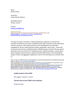
528
JOURNAL OF ATMOSPHERIC AND OCEANIC TECHNOLOGY
VOLUME 32
Variational Estimation of Wave-Affected Parameters in a Two-Equation
Turbulence Model
XUEFENG ZHANG, GUIJUN HAN, DONG LI, XINRONG WU, AND WEI LI
Key Laboratory of Marine Environmental Information Technology, National Marine Data and Information
Service, State Oceanic Administration, Tianjin, China
PETER C. CHU
Naval Ocean Analysis and Prediction Laboratory, Department of Oceanography, Naval Postgraduate
School, Monterey, California
(Manuscript received 22 April 2014, in final form 19 November 2014)
ABSTRACT
A variational method is used to estimate wave-affected parameters in a two-equation turbulence model
with assimilation of temperature data into an ocean boundary layer model. Enhancement of turbulent kinetic
energy dissipation due to breaking waves is considered. The Mellor–Yamada level 2.5 turbulence closure
scheme (MY2.5) with the two uncertain wave-affected parameters (wave energy factor a and Charnock
coefficient b) is selected as the two-equation turbulence model for this study. Two types of experiments are
conducted. First, within an identical synthetic experiment framework, the upper-layer temperature ‘‘observations’’
in summer generated by a ‘‘truth’’ model are assimilated into a biased simulation model to investigate if (a, b) can
be successfully estimated using the variational method. Second, real temperature profiles from Ocean Weather
Station Papa are assimilated into the biased simulation model to obtain the optimal wave-affected parameters. With the optimally estimated parameters, the upper-layer temperature can be well predicted. Furthermore, the horizontal distribution of the wave-affected parameters employed in a high-order turbulence
closure scheme can be estimated optimally by using the four-dimensional variational method that assimilates
the upper-layer available temperature data into an ocean general circulation model.
1. Introduction
Observations (Kitaigorodskii and Lumley 1983; Thorpe
1984; Anis and Moum 1992; Terray et al. 1996; Drennan
et al. 1996; Babanin 2006; Kantha et al. 2010) show that
the dissipation of turbulent kinetic energy (TKE) is
enhanced greatly near the sea surface by surface gravity
waves under nonbreaking (including nonbreaking wave
turbulence and Langmuir turbulence) and breaking
waves. The breaking-wave-induced mixing has been
broadly implemented into ocean circulation and mixing
models (e.g., Mellor and Blumberg 2004). On the basis
of the observational evidence of the surface wave
breaking (Osborn et al. 1992; Agrawal et al. 1992),
Corresponding author address: Dr. Xuefeng Zhang, Key Laboratory
of Marine Environmental Information Technology, National Marine Data and Information Service, State Oceanic Administration,
93 Liuwei Rd., Hedong District, Tianjin 300171, China.
E-mail: [email protected]
DOI: 10.1175/JTECH-D-14-00087.1
Ó 2015 American Meteorological Society
Terray et al. (1996) suggested a three-layer structure:
The first layer (from the surface) is a wave-enhanced
layer with the depth on the same order as the significant
wave height, and the energy dissipation rate proportional to z23 (z denotes the vertical distance from the
sea surface), which is twice faster than the classical walllayer dissipation. The second layer is the transition layer
below the breaking zone (depth about 6z0; z0 is the
surface roughness length) (Craig and Banner 1994), with
the energy dissipation rate proportional to z22. The
third layer is the classic wall layer with the energy dissipation rate proportional to depth z21.
To model the wave-breaking-enhanced turbulence
near the sea surface layer, Craig and Banner (1994) and
Craig (1996) imposed a surface diffusion boundary condition on the turbulent kinetic energy equation (CB
boundary condition) in the Mellor–Yamada (MY) turbulence closure model (1982). Burchard (2001b) simulated a wave-enhanced layer under breaking surface
waves with a two-equation turbulence model including
MARCH 2015
529
ZHANG ET AL.
the CB boundary condition. Mellor and Blumberg
(2004) developed a wave-enhanced parameterization
scheme with the CB boundary condition to overcome
a weakness of the MY turbulence closure model that
produces a shallower surface boundary layer and higher
surface temperature during summertime warming in
comparison to the observations (Martin 1985). Zhang
et al. (2011a,b) identified the effect of breaking surface
waves on upper-ocean boundary layer deepening in the
Yellow Sea in summer utilizing the Princeton Ocean
Model generalized coordinate system (POMgcs; Ezer
and Mellor 2004). A well-mixed temperature surface
layer in the Yellow Sea can be reconstructed successfully when the breaking-wave-enhanced turbulent mixing is considered.
In addition to the wave breaking, other wave-related
processes are also important in modulating the upper
mixed layer, such as the nonbreaking wave (Babanin
and Haus 2009) and the Langmuir turbulence (Belcher
et al. 2012). Some studies indicate that the effect of wave
breaking on the upper-level turbulence is significant
within the depth comparable to the wave height (Terray
et al. 1996). However, for a deeper mixed layer, the
impact of wave breaking would be small and the effect of
Langmuir circulation and nonbreaking wave becomes
important (Babanin 2006).
Uncertain wave-affected parameters exist in modeling wave-induced turbulence (nonbreaking or breaking
waves), such as the critical value of the wave Reynolds
number Recr in nonbreaking waves and the wave energy
factor a and the Charnock coefficient b in breaking
waves. These parameters are usually determined empirically or adjusted artificially. Studies have shown
successful parameter estimation with a dynamical model
using variational optimal control techniques (Derber
1987; Le Dimet and Talagrand 1986). For example, Yu
and O’Brien (1991, 1992) used the variational method to
assimilate meteorological and oceanographic observations into a one-dimensional oceanic Ekman layer
model, to estimate the drag coefficient and the oceanic
eddy viscosity profile and to investigate the effect of
initial condition on the variational parameter estimation. Zhang et al. (2003) showed the capability of fourdimensional variational data assimilation (4D-VAR) in
estimating uncertain parameters in numerical models.
Peng and Xie (2006) developed a tangent linear model
and an adjoint model of three-dimensional POM to
construct a 4D-VAR algorithm for coastal ocean prediction. Effective error correction was found in initial
conditions and wind stress in the storm surge simulation
(Peng et al. 2007), and the drag coefficient was estimated
in the storm surge prediction using the adjoint model of
the three-dimensional POM (Peng et al. 2013). Peng and
Xie (2006) also pointed out that it is still an open issue as
to whether it is meaningful to linearize the turbulence
closure scheme in an atmospheric or oceanic model due
to the high nonlinearity and discontinuity of the vertical
turbulence. The nonphysical noise might be produced,
and thus lead to numerical instability during the process
of linearizing the turbulence closure scheme. They applied a simple but efficient way of avoiding the noise
problem through neglecting the variation of the vertical
diffusion coefficients in the linearization of the vertical
turbulence scheme.
Despite earlier studies on the parameter estimation
and model verification (e.g., Chu et al. 2001), the adjoint
model of the turbulence closure scheme has not yet been
thoroughly investigated with either nonwave breaking
or wave breaking. Determination of wave-affected parameters in the turbulent mixing due to breaking waves
using the variation method is selected as the major objective of this study. First, the upper-layer temperature
‘‘observations’’ are produced by a ‘‘perfect’’ model.
Second, a biased assimilation is conducted to identify
the capability of the variational method to optimally
estimate the wave-affected parameters in the MY2.5
turbulence closure scheme. Third, the real temperature
profiles at Ocean Weather Station Papa (OWS Papa)
are assimilated into the ocean model to obtain the optimal wave-affected parameters.
2. Ocean boundary layer model
a. Mean equations and second-moment closure
Let (x, y) be the horizontal coordinates, z the vertical
coordinate, and t the time. Following D’Alessio et al.
(1998), equations governing the mean flow, temperature, and salinity in a horizontally homogeneous ocean
boundary layer are given by
›u
›
›u
2fy 5
KM
,
›t
›z
›z
›y
›
›y
1 fu 5
KM
,
›t
›z
›z
›T ›
›T
›R
5
KH
2 ,
›t ›z
›z
›z
›S ›
›S
5
KH
,
›t ›z
›z
(1)
where u, y are the velocity components in the x, y directions, respectively; T is the potential temperature; S is
the salinity; f is the Coriolis parameter; and KM and KH
are the vertical mixing coefficients for momentum and
tracers, respectively.
530
JOURNAL OF ATMOSPHERIC AND OCEANIC TECHNOLOGY
The MY2.5 turbulence closure scheme, widely used in
ocean models such as POM and the Regional Ocean
Modeling System (ROMS), is a two-equation turbulence model,
(
" )
2 #
›q2
›u 2
›y
g
›r q3
5 2 KM
1
1 KH 2
›z
›z
r0
›z B1 l
›t
›
›q2
Kq
, and
1
›z
›z
(2)
( " )
2#
›q2 l
›u 2
›y
g
›r q3 W
5 lE1 KM
1 KH 2
1
›t
›z
›z
r0
›z B1 l E1
›
›q2 l
Kq
,
1
›z
›z
(3)
where q2 is the turbulent kinetic energy times 2; l is the
turbulent macroscale; Kq is the vertical mixing coefficient for turbulence; and r and r0 are the density and
reference density, respectively,
L21 5 (h 2 z)21 1 (H 1 z)21 ,
W 5 1 1 E2 (l/kL)2 ,
where k (50.41) is the von Kármán constant, H is
the water depth, h is the free-surface elevation, and
E1, E2, and B1 are empirical constants. The turbulent
energy and macroscale equations are closed by
KM 5 lqSM ,
KH 5 lqSH ,
Kq 5 lqSq ,
(4)
where SM and SH are the stability functions.
b. Wave-affected parameters
Wave-affected parameters are included in the surface
boundary conditions of the two-equation turbulence
model. The first one is the CB boundary condition for q2
(Craig and Banner 1994),
Kq
›q2
›z
5 2au3t ,
z 5 0,
(5)
where ut is the water-side friction velocity and a is
‘‘wave energy factor.’’ The second one is for the turbulent macroscale l (Terray et al. 1996, 1999),
l 5 max(kzw , lz ) ,
(6)
where lz is the ‘‘conventional’’ empirical length scale,
which is calculated prognostically by the MY2.5 turbulence closure scheme; and zw is the wave-related surface
VOLUME 32
roughness length, which denotes the relevant scale of
turbulence.
In the absence of surface waves, both a and zw at the
surface are set as zero in the MY2.5 turbulent closure
scheme (Blumberg and Mellor 1987). However, when
the effect of surface waves is considered, both a and zw
appear as constants or vary with the states of surface
waves. Craig and Banner (1994) set a as 100 for wave
ages embracing very young wind seas to fully developed situations. Terray et al. (1996) indicates that
a 5 150 is an adapted value under breaking waves.
Kraus and Turner (1967), Denman and Miyake (1973),
and Gaspar (1988) also choose different values of a in
their studies.
Terray et al. (1996), Burchard (2001a), and Umlauf
and Burchard (2003) suggest that zw is the same order
as the significant wave height (Hs). Further, Mellor and
Blumberg (2004) summarized the work of Donelan
(1990), Smith et al. (1992), and Janssen (2001), and
obtained
zw 5 ( b 3 105 )
u2t
,
g
(7)
where g is the gravitational acceleration, and b is the
Charnock parameter (Chu and Cheng 2007), which
varies from b 5 2 (Stacey 1999) and b 5 0.32 (Jones
and Monismith 2008) to b 5 0.56 (Carniel et al. 2009)
to obtain the best performance in each numerical
simulation. Mellor and Blumberg (2004) suggested
that b ; O(1) is deemed correct under breaking waves.
Stacey (1999) also indicated that b ; O(10) is too big
a value to describe the surface boundary condition for
the turbulent kinetic energy. It should be noted that b
does not have to be so large if the other wave-induced
mixing process is included in the models (Zhang et al.
2012).
c. Boundary conditions
The surface boundary conditions for q2 and l are given
by Eqs. (5) and (6). The bottom boundary conditions of
q2 and l are given by
q2 5 B12/3 u2tb ,
l 5 kz0 ,
and
(8)
(9)
respectively, where B1 5 16.6 (Blumberg and Mellor
1987) and utb is the friction velocity associated with the
bottom frictional stress. The surface and bottom
boundary conditions of the mean flow and tracers are
represented by
MARCH 2015
531
ZHANG ET AL.
›T
Q
5
›z r0 Cp
9
>
>
>
>
>
>
>
>
>
=
S 5 Sobs
at z 5 0
>
t wx t wy
›u ›y
>
>
KM
,
,
5
, (twx , t wy ) 5 Cw u10 (ux , uy ) >
>
>
›z ›z
r0 r 0
>
>
>
;
23
Cw 5 (0:75 1 0:067ju10 j) 3 10
(10)
and
9
›T
>
>
50
>
>
›z
>
>
>
>
>
›S
>
>
>
50
>
>
›z
=
at z 5 2H(x) ,
t
t
›u ›y
by
,
5 bx ,
, (t bx , t by ) 5 Cd ub (ubx , uby ) >
KM
>
>
>
›z ›z
r0 r0
>
>
>
"
#
>
>
>
2
>
k
>
>
, 0:0025
Cd 5 max
>
;
2
ln(z/z0 )
where Q is the surface net heat flux; Cp is the specific heat;
Sobs is the observation of the sea surface salinity; t wx and
t wy are the x and y components of the wind stress, respectively; u10 is the wind velocity at 10 m; ux and uy are x
and y components of u10 , respectively; t bx and t by are the x
and y components of the bottom frictional stress, respectively; ub is the bottom velocity; ubx and uby are the x
and y components of ub, respectively; Cw and Cd are drag
coefficients of the wind stress and the bottom stress, respectively; and z0 is the bottom roughness parameter, taken
as 0.01 m.
3. Variational approach
a. The variational theory within the least squares
framework
(11)
and F is the differential operator. The symbol h i represents the inner product in the Euclidean space. Term
W is the weight matrix. Term Xobs is the observation,
and C is the projection operator from the model space to
the observational space. Let
J( popt ) 5 min( p) .
The optimal control variable popt is obtained from
$J( popt ) 5 0
with respect to all control variables. Here, $ is the gradient operator. The process for the variational analysis
can be outlined as follows:
where p is the vector of the control variables, X is the
solution of the dynamical model
(i) Define a concrete cost function that reflects the
misfit between the control variables and the available observations.
(ii) Calculate the value of the cost function J( p)
through integrating the dynamical model with
a fixed time step.
(iii) Calculate the gradients of the cost function with
respect to all control variables, $J( p).
(iv) Minimize the cost function through a minimization
algorithm according to the value of J( p) and $J( p).
(v) Estimate the optimal control variables popt according to the convergence criterion of the process of
the minimization.
dX
5 F(X) ,
dt
For executing the above-described process of the variational analysis (i)–(v), $J( p) should be obtained in
The purpose of the variational analysis is to seek the
optimal control variables by minimizing a well-defined
cost function, in which a dynamical model including all
the control variables is regarded as the strong constraints
of the cost function. Within the least squares framework,
a general form of the cost function can be defined as
1
J( p) 5
2
ðT
0
hW(CX 2 Xobs ), (CX 2 Xobs )i , (12)
532
JOURNAL OF ATMOSPHERIC AND OCEANIC TECHNOLOGY
advance, and in general, it is calculated by the adjoint
model of the linearized dynamical model. To the first
order the Taylor expansion of J( p) is given by
J( p) 5 J( p0 ) 1 dJ( p) ,
(13)
where dJ( p) is the variation of J( p).On the one hand,
dJ( p) is given by the definition of the variation:
dJ( p) 5
ðT
0
h$X J( p0 ), dXi .
(14)
On the other hand, dJ( p) can also be written according
to Eq. (12),
ðT ›C
W
dX, CX 2 Xobs
›X
0
ð 1 T
›C
dX .
W(CX 2 Xobs ),
1
2 0
›X
1
dJ( p) 5
2
(15)
With the symmetry of the inner product as well as
a constant W matrix, Eq. (15) can be rewritten as
dJ( p) 5
ðT ›C
dX .
W(CX 2 Xobs ),
›X
0
(16)
Let ›C/›X 5 A(X), thus Eq. (16) can be given as
dJ( p) 5
ðT
0
hW(CX 2 Xobs ), A(X)dXi ,
(17)
where A(X) is the tangent linear operator. Equation
(17) can be transposed according to the definition of the
adjoint operator,
dJ( p) 5
ðT
0
hWA*(X)(CX 2 Xobs ), dXi ,
(18)
where A*(X) is the adjoint operator of A(X). Compared
with Eq. (14), $X J( p0 ) can be described by
$X J( p0 ) 5 WA*(X)(CX 2 Xobs ) .
(19)
VOLUME 32
calculated using the adjoint model. The difference
CX 2 Xobs is regarded as an external forcing of the
adjoint model.
The general form of the adjoint model can be found in
appendix A. The discretized adjoint model that computes the gradient of the cost function can be developed
directly from the discretized dynamical model including
Eqs. (1)–(11). In practical application, the source code
of the adjoint model is constructed by combining the
Tangent and Adjoint Model Compiler (TAMC) developed by Giering and Kaminski (1998) and a handcoding correction. First, the adjoint code is generated by
TAMC to avoid human errors and negligence, which are
extremely easy to happen during the direct coding.
Second, hand-coding correction is conducted to correct
the AMC-generated code and to control the adjoint
code structure. The errors in the adjoint code, which are
induced from some irregular expressions of the forward
numerical model, such as the partial array assignment
and iterative use of intermediate arrays, are corrected
through the hand coding. Finally, through the handcoding correction, values of many intermediate results
in the adjoint model are recorded into memory instead
of recomputed to shorten the run time of the adjoint
model, and some local variables and arrays are transferred to global attribute to improve the run efficiency of
the adjoint model.
Once the cost function and its gradient are obtained
from the dynamical model and its associated adjoint
model, the minimization process is implemented to
minimize the cost function through iterating the values
of the control variables (T n, T n21, a, and b) with the
limited-memory Broyden–Fletcher–Glodfarb–Shanno
(BFGS) quasi-Newton minimization algorithm (Liu
and Nocedal 1989). During the minimization process,
the maximum of a is set to 1000, and the maximum of b
is set to 10 according to Mellor and Blumberg (2004)
and Stacey (1999). The minima of the two waveaffected parameters are set to zero to keep realistic
physical conditions. The minimization process is repeated until the convergence criterion of the gradient is
reached. At that time, the optimal values of the control
variables are obtained.
b. The adjoint model
According to Eq. (19), the gradient of the cost function with respect to the control variables can be
c. Cost function
In this study, the cost function is defined by
1
1 n21
n
n
n21
J(T n , T n21 , a, b) 5 (T n 2 Tbn )T B21
2 Tbn21 )T B21
2 Tbn21 )
1 (T 2 Tb ) 1 (T
2 (T
2
2
1 M N
1 å å [Tj,i (a, b) 2 Tobs ]T R21 [Tj,i (a, b) 2 Tobs ] ,
2 j51 i51
(20)
MARCH 2015
533
ZHANG ET AL.
TABLE 1. All assimilation experiments and simulations within the identical synthetic experiment framework.
Name
Description
Truth model simulation
a 5 200
b 52
a 5 100
b 51
Parameter estimation
Parameter estimation
Parameter estimation with the perfect
initial fields derived from the truth
model simulation
Parameter estimation with the biased
initial fields derived from the biased
simulation
Biased simulation
PE
PE_SST
PE_b_TI
PE_b_BI
where the first two terms on the right side represent the
background error terms that measure the misfit between
the model’s initial field and the background field. Terms
T n and T n21 are the initial temperature values at the nth
and (n 2 1)th time steps, respectively, which will be
estimated optimally via the variational method. Terms
Tbn and Tbn21 are the background temperature values at
the nth and (n 2 1)th time steps, respectively, which can
be derived from the model run. Both temperatures at
the two consecutive time steps are considered as the
control variables due to the utilization of the leapfrog
time differencing scheme with the Asselin–Robert time
filter (Robert 1966). Otherwise, initial shocks of the
model states are likely to be produced during the variational estimation because of the inconsistence of the
initial values at the two time steps. Terms B1 and B2 are
the error covariance for T n and T n21 , respectively; for
simplicity, both B1 and B2 use diagonal matrices, whose
Control
variables
Assimilation
windows
Assimilation
period
Assimilation
depth
—
—
—
—
—
—
—
—
T n, T n21, a, b
T n, T n21, a, b
b
1 day
1 day
1 day
1 day
1 day
1 day
30 m
Sea surface
30 m
b
1 day
1 day
30 m
values of the diagonal components are set to 1024 in this
study. The third term denotes the observation of the
temperature at certain time intervals within the assimilation window, where Tj,i and Tobs are the simulated and
observed temperature at location i and time level j, respectively. Terms N and M are the number of grid points
over the ocean and the number of time levels of observations, respectively. Term R is the error covariance for
the observations, which also uses the same diagonal
matrix as that of B1.
Wave-affected parameters a and b are expressed
implicitly in Eq. (20), which are regarded as the independent variables of Tj,i . Therefore, the value of the
cost function can be obtained when the model integrates
for n time steps with the known initial values of T n , T n21 ,
a, and b. The cost function has the following form if the
wave-affected parameters a and b have background
values (ab, bb, respectively):
1
1 n21
n
n
n21
2 Tbn21 )T B21
2 Tbn21 )
J(T n , T n21 , a, b) 5 (T n 2 Tbn )T B21
1 (T 2 Tb ) 1 (T
2 (T
2
2
1 M n
1
1
1 å å [Tj,i (a, b) 2 Tobs ]T R21 [Tj,i (a, b) 2 Tobs ] 1 Ka (a 2 ab )2 1 Kb (b 2 bb )2 ,
2 j i
2
2
where Ka and Kb are coefficients controlling the best fits
for data. In this study, we use the first form of the cost
function [Eq. (20)] for avoiding the complexity of the
cost function.
4. Synthetic experiments
a. Truth model simulation
Table 1 lists all the assimilation experiments and
model simulations within an identical synthetic experiment framework. The truth model consists of Eqs. (1)–
(3) with a 5 200 and b 5 2. All six equations from Eqs.
(21)
(1)–(3) are discretized using the same implicit method as
POM. The maximum depth is set to 250 m, with 60 vertical levels. The first 20 vertical levels are 0.0, 0.5, 1.0, 1.5,
2.0, 4.0, 6.0, 8.0, 10.0, 12.0, 14.0, 16.0, 18.0, 20.0, 22.0, 24.0,
26.0, 28.0, 30.0, and 35.0 m. The time step is 1 h. The
model initial state is from 1 January 1961, including
temperature and salinity, derived from the real observation at OWS Papa. The model is forced by the observational 10-min momentum and heat fluxes acquired online
from (http://www.pmel.noaa.gov/OCS/Papa).
Starting from the initial conditions (1 January 1961),
the truth model is run for 6 yr to generate a time series of
534
JOURNAL OF ATMOSPHERIC AND OCEANIC TECHNOLOGY
VOLUME 32
FIG. 1. Daily temperature in 1966 at (a) 0, (b) 10, (c) 20, and (d) 30 m at OWS Papa with the truth model simulation
(solid curve) and the biased simulation (dashed curve).
the truth with the first 5 yr as the spinup period. The time
of the observations of T is from 1 to 30 August 1966. The
observations of T are produced through sampling the
truth states at 1-h observational frequencies. The observation locations of T are consistent with those of the
model vertical grids.
b. Biased simulation
The biased simulation uses the same truth model, but
with different parameter settings. Therefore, the difference between the biased simulation and the truth
model leads to the effect of the incorrect parameter
settings. Figure 1 shows the simulated daily temperature
at OWS Papa in 1966. The sea surface temperature
(SST) from the biased simulation with (a, b) 5 (100, 1) is
higher than that by the truth model simulation with
(a, b) 5 (200, 2), and the maximum difference of the
SST between the two simulations occurs in summer,
namely, from the 200th day to the 240th day (solid line vs
dashed line in Fig. 1a). An obvious difference of the
temperature at 10-m depth in the two simulations also
remains (Fig. 1b). The wave-affected parameters are
half smaller in the biased simulation than in the truth
model simulation, which suggests that the turbulent kinetic energy is too weak to mix the surface and subsurface water well in the biased simulation. After the
240th day (fall and winter), the temperature decreases
gradually due to the convective mixing induced by the
surface cooling. The temperatures at the surface and 10-m
depth in the biased simulation remain higher than the
counterpart in the truth model simulation due to the
insufficient wave-enhanced mixing in the biased simulation. Below 20 m, the effect of the wave-affected parameters on the temperature is not evident in summer
(solid line vs dashed line in Figs. 1c and 1d), which indicates that the turbulent kinetic energy generated by the
breaking surface gravity waves is dissipated only near the
sea surface and does not penetrate into the deeper waters.
The maximum difference in temperature at 30 m from the
two simulations occurs in the fall (after the 250th day)
with the temperature higher in the biased simulation than
in the truth model simulation. Although the waveaffected parameters do not directly affect the temperature in the deeper layers in summer, it can affect the
temperature indirectly by the SST due to the subsequent
convective cooling in autumn and winter. Thus, the waveaffected parameters directly impact the temperature near
the sea surface in summer, and indirectly impact the
temperature in the deeper layers in autumn and winter.
We intend to investigate if the wave-affected parameters in a two-equation turbulence model can be estimated effectively through assimilating the temperature
data into an ocean boundary layer model with the variational method. In addition, we want to understand how
well the model state estimation/forecast can be improved
through the estimated wave-affected parameters. In the
next subsection, a series of synthetic experiments are
carried out to address the issues.
c. Correctness test of the gradient
The code of the adjoint model is produced directly
through the TAMC (of course, a hand-coding correction
MARCH 2015
ZHANG ET AL.
535
FIG. 2. The correctness test of the gradient with respect to (a) a and (b) b.
is necessary after that). According to the Taylor expression, one has
lim u(«) 5 lim
«/0
«/0
J[x0 2 «$J(x0 )] 2 J(x0 )
’ 1, (22)
2«h$J(x0 ), $J(x0 )i
where x0 is any control variable and the symbol h i represents the inner product. Figure 2 shows the correctness
test of the gradient of the cost function with respect to
a and b using Eq. (22). With respect to a, u(«) converges
to 1 as « decreases from 1023 to 1028, and decreases from
1 to 0.38 as « decreases from 1028 to 10210, which indicates the dominance of the computational errors in
u(«). With respect to b, u(«) converges to 1 as « decreases
from 1026. Therefore, the adjoint coding is valid.
five iterations, and it keeps the low value (0.8) steadily
after the fifth iteration (Fig. 4a). However, the norm of
the gradient oscillates dramatically to search the optimal
declining direction of the gradients. The norm of the gradient becomes stable after the 130th iteration (Fig. 4b).
The minimization process stops after 180 iterations, indicating the local minima of the wave-affected parameters
for that day.
Figure 5 depicts the temporal variations of the natural logarithm of the cost function at OWS Papa from
d. Parameter estimation
Figure 3 shows the time series of a and b during the
parameter estimation (PE) described in Table 1, where
both the assimilation window and assimilation period
are set to 24 h and the assimilation depth is set to 30 m.
Therefore, the processes (ii)–(vii) described by appendix C are executed 30 times to obtain time series of a and
b from 1 to 30 August 1966. Figure 3b shows that b
converges to its truth value (dashed line) after 9 days,
while a converges to its truth value (dashed line in
Fig. 3a) after about 15 days. Results show the waveaffected parameters in the high-order turbulent model
can be estimated successfully using the upper-layer
temperature observations through the variational control technique. For each cycle of the parameter estimation in the 30 days, the process of the minimization is
iterated until the convergence criterion of the gradient is
satisfied. Figure 4 shows the dependence of the cost
function and the norm of the gradient on the number of
iterations on 2 August 1966. The value of the cost
function decreases rapidly from 4.3 to 0.8 within the first
FIG. 3. Time series of the estimated wave-effected parameters
(a) a and (b) b for PE from 1 to 30 Aug 1966 (solid curve), where
both the assimilation window and the assimilation period are 1 day
and the depth of the assimilation is 30 m. Here, the dashes curves
show the truth (a, b) values.
536
JOURNAL OF ATMOSPHERIC AND OCEANIC TECHNOLOGY
VOLUME 32
FIG. 5. Temporal variations of the natural logarithm of the cost
function at OWS Papa from 1 to 30 Aug 1966. Here, the red, blue,
and black curves are the total, background, and observation terms
of the cost function.
FIG. 4. Dependence of (a) the cost function and (b) the norm of the
gradient on the number of iterations on 2 Aug 1966.
1 to 30 August 1966. The cost function (red line) decreases dramatically in the first 5 days and then decreases
gently in the following 25 days. Both the background
term (blue line in Fig. 5) and the observation term (black
line in Fig. 5) of the cost function have a similar pattern
with the total cost function. The two terms almost
converge to the same value after the 10th day, indicating the estimated initial temperature fields reach
a balance between the background temperature and
the observation.
The temporally varying wave-effected parameters
(a, b) estimated from their different initial values on 1
August 1966 (Fig. 6) converge to their truth values
within one month through the parameter optimization
with the variational approach. It clearly shows that the
variational assimilation approach is feasible for the
wave-affected parameter optimization with different
initial parameter values.
To evaluate the effect of the noise in the temperature
observation on the wave-affected parameter estimation,
FIG. 6. Time series of the estimated wave-effected parameters (a) a and (b) b for different initial parameter
values from 1 to 30 Aug 1966, where both the assimilation window and the assimilation period are 1 day and the
depth of the assimilation is 30 m. Black, blue, green, yellow, red, pink, purple, orange, and gray solid lines in (a) and
the corresponding dashed lines in (b) show values of (a, b) 5 (0, 0), (100, 2), (100, 3), (200, 1), (200, 3), (300, 1),
(300, 2), (300, 3), and (400, 4) respectively.
MARCH 2015
537
ZHANG ET AL.
TABLE 2. Dependence of the optimally estimated (a, b) on the standard deviation of temperature observation.
Std dev of temperature
observation
Estimated
value of a
Estimated
value of b
Relative error
of a (%)
Relative error
of b (%)
1023
1022
0.05
0.1
0.5
206.125
167.343
120.033
100.096
100.068
1.982
2.098
2.114
1.889
0.866
96.9
83.6
60.0
50.0
50.0
99.1
95.1
94.3
94.5
43.3
based on the PE experiment, the white noises with different standard deviation are added to the temperature
observation. Table 2 shows the dependence of the optimally estimated (a, b) on the error standard deviation
of the temperature observation. The relative error of
optimally estimated a decreases from 96.9% to 60%,
and the relative error of the optimally estimated b decreases from 99.1% to 94.3% as the error standard deviation in the temperature observation increases from
0.001 to 0.05 K. It implies that the effect of observational
noise on the estimation is more severe on a than on b,
which means that it is more difficult to pick up the
positive signal when the noise dominates the cost function and the corresponding gradients during the parameter estimation of a. When the standard deviation of
the temperature observation increases to 0.5 K, both
relative errors of the optimally estimated a and b are
below 50%, which indicates that the level of the noise is
not acceptable for assimilation purposes.
To determine if the wave-affected parameters can be
estimated correctly using only the SST data, the second
assimilation experiment, PE_SST, is conducted, in
which only the SST observations are assimilated into the
biased simulation model. Neither a (Fig. 7a) nor b
(Fig. 7b) reaches their truth values (dashed curve) due to
the poor constraint of the observation. When only the
SST observations are assimilated, the subsurface temperature cannot be estimated accurately. Under this
condition, the two parameters will be adjusted to the
optimal values to fit the inaccurate temperature values
to the greatest extent within a fixed time window, rather
than converge to truth values. Therefore, the subsurface
temperature observations are essential for estimating a
and b reasonably well.
The dependence of the optimally estimated a (Fig. 8a)
and b (Fig. 8b) on the assimilation window and assimilation period is investigated using different values from
1 to 30 August 1966 (Fig. 8). When the assimilation
window and the assimilation period are 48 and 72 h,
respectively, both parameters converge to their respective truth values (see black and blue lines in Figs. 8a
and 8b). However, when the assimilation window and
the assimilation period reach 96 and 120 h, respectively,
neither a nor b converges to their truth values within
one month, which can be seen from the red and pink
lines in Figs. 8a and 8b. It clearly shows that the parameter updating with the observation can improve the
state estimation of the next cycle, and that the improved
state estimation further enhances the quality of parameter estimation for the next cycle of parameter correction. When the assimilation window and the assimilation
period are set to 120 h, the state-parameter optimization
is performed only in six cycles within one month. Although the cost function decreases gradually, which can
be seen from the dashed curve in Fig. 9, the control
variables (the initial temperature T and the two parameters a, b) are not estimated reasonably well. In
contrast, when the assimilation window and the assimilation period are set to 24 h, just as in the PE experiment,
the state-parameter optimization can be performed in 30
cycles within one month, and the cost function can reach
quasi equilibrium after 10 days (solid curve in Fig. 9).
FIG. 7. As in Fig. 3, but for PE_SST, where only the SST observations
are assimilated.
538
JOURNAL OF ATMOSPHERIC AND OCEANIC TECHNOLOGY
VOLUME 32
FIG. 8. Time series of the estimated wave-effected parameters (a) a and (b) b for a different assimilation window
and assimilation period from 1 to 30 Aug 1966, where the depth of the assimilation is 30 m. Black, blue, red, and pink
solid lines in (a) and (b) show the assimilation period and are 48, 72, 96, and 120 h.
It should be noted that the initial temperature values
are regarded as not only the control variables being estimated but also the background temperature values of
the cost function [see Eq. (20)] in the current minimization cycle. The incorrect convergence of (a, b) suggests
that the initial temperature field (the background temperature values) in the current cycle is not adjusted well
enough, which is regarded as the source of noise during
parameter estimation using the variational method.
Therefore, it is hard to obtain the accurate values of
(a, b) before the state variables (T n and T n21) attain the
adequate accuracy. To better understand the issue, two
other experiments are carried out, in which b is regarded
as the only control variable. The experiment PE_b_TI
described in Table 1 uses the ‘‘perfect’’ initial field that is
generated by the truth model with the truth values of a
and b; the other experiment, PE_b_BI, uses the ‘‘biased’’
initial field that is generated by the biased simulation
with the biased values of a and b. Table 3 shows the
evolution of the cost function, the norm of the projected
gradient, and the value of b with respect to the number of
iterations in PE_b_TI. The parameter b reaches its truth
value at the third iteration. The convergence criterion of
the gradient is satisfied at the fourth iteration. However,
b estimated from PE_b_BI cannot converge to its truth
value (Table 4). After the convergence criterion of the
gradient is satisfied at the sixth iteration, b reaches
3.3023 35, which is different from the truth value of 2.0.
Although b from PE_b_BI cannot converge to its truth
value, it reaches its optimal value to compensate for
the error derived from the biased initial field during
minimizing the model-observation misfit.
In fact, in a 3D ocean circulation model, model biases
arise from the imperfect dynamical core and empirical
physical schemes even if the initial field is perfect. With
a biased initial field alone, one expects that the parameter
optimization can compensate for both the numerical and
physical deficiencies of the numerical model and enhance
the performance of the model simulation to a certain
degree. In this situation, parameters can only converge to
their optimal value, instead of the truth values. In the next
section, real temperature profiles from OWS Papa will be
assimilated into the assimilation model to obtain the
optimal wave-affected parameters (a, b).
5. Real experiment
OWS Papa is located in the North Pacific at 508N,
1458W, where the currents are relatively weak and the
FIG. 9. Temporal variations of the natural logarithm of the cost
function at OWS Papa from 1 to 30 Aug 1966. The solid and dashed
curves represent PE and PE_5d, respectively, with black dots denoting the time that observations are assimilated.
MARCH 2015
539
ZHANG ET AL.
TABLE 3. Evolution of the cost function, the norm of the projected gradient, and the value of b with respect to the number of
iterations for the direct perturbed method with the perfect initial
field.
Iteration
step
Cost
function
Norm of the
projected gradient
Value
of b
0
1
2
3
4
5.881
1.354 3 1025
2.631 3 1029
7.441 3 10217
5.056 3 10217
2.097
7.406 3 1022
1.032 3 1023
3.042 3 1027
5.693 3 1029
1.0
2.000 365
2.000 005
2.000 000
1.999 999
local mixing modulates mainly the dynamical process in
the upper ocean in summer. The observed temperature
profiles from 1 to 31 August 1966 at the site have a 3-h
interval and a coarser vertical resolution (5 m) than the
model grid points. There are seven observational layers
totally in the upper 30 m, namely, 0, 5, 10, 15, 20, 25, and
30 m. Linear interpolation is used to fill the spatial gap
between the modeled data and the observational data.
Table 5 lists all the assimilation experiments and
model simulations within the real experiment framework. First, a control run without assimilating any observational data is called control (CTRL) to serve as the
reference for the evaluation of assimilation experiments. The initial temperature and salinity are taken
from those at 0000 UTC 1 January 1961 and linearly
interpolated to model grids. The high-resolution (10
min) surface-observed data (momentum and net heat
fluxes) at the site are used to force the model. Figure 10a
shows the daily observed (red curve) and simulated sea
surface temperature from CTRL (black dashed curve)
at OWS Papa on August 1966. The simulated SST is
higher than the observed SST by about 38C (black
dashed curve vs red curve). At the same time, the simulated mixed layer depth from CTRL is shallower than
the observation by more than 10 m (black dashed curve
vs red curve in Fig. 10b). The optimal values of (a, b) are
estimated with the variational method to mitigate the
bias between the model and the observation using the
real summer temperature data.
TABLE 4. As in Table 3, but with the biased initial field.
Iteration
step
Cost
function
Norm of the
projected gradient
Value
of b
0
1
2
3
4
5
6
2.319 3 1022
1.072 3 1022
1.071 3 1022
1.071 3 1022
1.071 3 1022
1.071 3 1022
1.071 3 1022
4.819
3.351
1.234
9.003 3 1023
1.982 3 1023
6.043 3 1026
3.627 3 1026
1.0
3.350 811
3.317 216
3.301 275
3.302 359
3.302 335
3.302 335
The real parameter estimation (RPE) is described in
the second row of Table 5. The initial field is generated
from the results on 1 August 1966 simulated by the truth
model in the above-mentioned synthetic experiments.
The initial values of (a, b) are also consistent with those
in the truth model simulation. The length of both the
assimilation window and the assimilation period are set
to 3 days (8 real observational temperature profiles in
each day, for a total of 24 profiles for 3 days) and the
assimilation depth is 30 m. The process of PE is similar to
the process described in section 3, but with the real
temperature observations at OWS Papa in August 1966.
Table 6 shows the evolution of the cost function, a, and b
with respect to the number of iterations for RPE. After
the eighth iteration, the normalized cost function decreases to 5% of its initial value. The optimal values of a
and b reach 107.48 and 3.98, respectively. The SST from
RPE has a significant improvement compared to the
simulated SST from CTRL (black solid curve vs black
dashed curve in Fig. 10a), whose values are basically
consistent with those of the observations (black solid
curve vs red curve in Fig. 10a). The mixed layer depth is
also more accurate from RPE than from CTRL
(Fig. 10b). However, some discrepancy in the mixed
layer depth still exists between RPE and the observation. This is because too many factors modulate the
complicated thermodynamic processes of the upper
mixed layer besides the surface gravity waves, such as
horizontal advection, internal waves, upwelling, and
entrainment. Many physical processes are not enclosed
TABLE 5. All the assimilation experiments and model simulations within the real experiment framework.
Name
Description
CTRL
Simulation with a 5 200 b 52
RPE
RSE_Po
Real parameter estimation
Simulation using the parameters
estimated by RPE
Simulation using the same
parameters as in CTRL
RSE_Pd
Control
variables
Assimilation
windows
Assimilation
period
Assimilation
depth
—
—
—
—
T n , T n21 , a, b
—
3 days
—
3 days
—
30 m
—
—
—
—
—
Initial fields
1 Aug 1966 from the truth
model simulation
Same as CTRL
31 Aug 1966, derived from
RPE
Same as RSE_Po
540
JOURNAL OF ATMOSPHERIC AND OCEANIC TECHNOLOGY
VOLUME 32
TABLE 6. Evolution of the cost function (a, b) with respect to the
number of iterations for the real assimilation.
Iteration
step
Normalized
cost function
Value
of a
Value
of b
1
2
3
4
5
6
7
8
1.0
0.52
0.26
0.29
0.26
0.14
0.17
0.05
107.12
107.45
107.61
107.97
107.39
107.48
107.52
107.54
4.40
4.44
4.37
4.23
3.79
3.86
3.96
3.98
vertically homogeneous. It indicates that the model performance can be effectively improved using the optimal
parameters. However, more accurate model simulations
are needed using the optimal values of parameters via the
variational methods repeated at certain time intervals
with more available observations.
FIG. 10. (a) SST and (b) mixed layer depth from CTRL (black
dashed curve) and RPE (black solid curve), and observations (red
solid curve) at OWS Papa from 1 to 30 Aug 1966. Horizontal axis
represents the day relative to 1 Aug 1966.
in the simple ocean boundary layer model. The optimal
values of the parameters can only compensate for some
model bias but not all. However, the result from RPE
indicates that the variational estimation of waveaffected parameters can indeed reduce model biases
and improve the model capability in the upper ocean.
To explore the impact of parameter estimation on
model simulation, two validation experiments, RSE_Po
and RSE_Pd, are conducted. The optimal parameters
estimated from RPE are used in RSE_Po, and the default values of the parameters from CTRL are used in
RSE_Pd. In addition, both experiments use the same
initial fields on 31 August 1966, which are derived from
RPE. Figure 11 shows the observed (red curve) and
simulated SST from RSE_Po (black solid curve) and
RSE_Pd (black dashed curve) at OWS Papa from 1 to 30
September 1966. The simulated SST is more consistent
with the observations from RSE_Po than from RSE_Pd.
The simulated twice-monthly averaged turbulent kinetic
energy q2 (Fig. 12a) and the vertical mixing coefficient
for temperature KH (Fig. 12b) at OWS Papa in September
1966 are much larger for all the depths in RSE_Po
(solid curve) than in RSE_Pd (dashed curve). The enhanced KH in the upper-30-m depth in RSE_Po, due to
the improvement of the turbulent kinetic energy calculation, mixes the momentum from the winds downward through the water column and makes it more
6. Discussion and conclusions
Wave-affected parameters in high-order turbulence
closure schemes can modulate distinctly the vertical
structure in the upper ocean. For improving the performance of the model in simulating the upper-ocean
mixed layer, it is essential to estimate the optimal values
of the wave-affected parameters using available observations deployed in the upper ocean through some robust data assimilation methods. It is known that one of
the advantages of the variational method is that it can
seek a posterior maximum likelihood solution of the
model parameters in terms of the best fitting of the
modeling trajectory to the observations by minimizing
a cost function that measures the distance between observations and model states within an appropriate minimization time window. Therefore, in this study, the
FIG. 11. SST from observations (red solid curve), RSE_Po (black
solid curve), and RSE_Pd (black dashed curve) at OWS Papa from
31 Aug to 30 Sep 1966. Horizontal axis represents the day relative
to 1 Aug 1966.
MARCH 2015
ZHANG ET AL.
541
FIG. 12. Vertical profiles of the simulated monthly averaged (a) 2 times q2 (m2 s22) and
(b) the vertical mixing coefficient for temperature KH (1023 m2 s21) from RSE_Po (solid curve)
and RSE_Pd (dashed curve) at OWS Papa in September 1966.
upper-layer temperature data are assimilated into an
ocean surface boundary layer model to tentatively estimate the wave-affected parameters (a, b) employed in
the MY2.5 two-equation turbulence model using the
variational method. Within an identical synthetic experiment framework, the ‘‘truth’’ values of the waveaffected parameters in the high-order turbulence model
can be retrieved successfully when the assimilation
window, the assimilation period, and the assimilation
depth are set appropriately. The observational temperature profiles at OWS Papa are also assimilated to correct the model bias arisen from multiple sources. By
fitting the model results to the observations using the
variational method, the optimal temperature field can
be obtained in the upper 30 m through adjusting the
wave-affected parameters to their optimal values.
Wave-affected parameter estimation using the variational method can compensate in part for the numerical
and physical deficiencies of the model in the upper
ocean. However, because of the existence of the deficiencies, the optimal values of the wave-affected parameters from the variational estimation might be not
close to so-called truth values, even far away from the
truth ones, which may induce that the upper-ocean
turbulent mixing is overestimated or underestimated.
The optimal values of the wave-affected parameters in
real applications are only applicable to the specific time
period, location, and model. Further, the optimal values
should vary temporally and spatially rather than being
constants, which can be obtained by using the variational methods repeatedly at certain time intervals and
the available observations (Peng et al. 2013). Although
the optimal values of the wave-affected parameters are
both model dependent (initial fields, time window of
assimilation, model configuration, etc.) and observation
dependent (sampling frequency, sampling errors, etc),
as is indicated by this study, they can indeed mitigate the
model biases from multiple sources, and obviously improve the performance of the model simulation.
Besides the wave-breaking parameters, other parameters in the wave-related processes can also be introduced into the model (which is compatible with those
pertinent to the wave breaking) to estimate their optimal values. For instance, it is well known that Langmuir
turbulence plays a key role in modulating the upperlayer mixing in the open sea. Recently, Harcourt (2013)
introduces two more parameters into a second-moment
closure turbulent model to describe the effect of the
542
JOURNAL OF ATMOSPHERIC AND OCEANIC TECHNOLOGY
Langmuir turbulence. One expects that the parameters
associated with the Langmuir turbulence can be estimated together with the wave-breaking parameters
using the variational method. Further, satellite remotesensed SST data and in situ temperature data (such
as the Argo floats) can provide a mass of temperature
observations in upper oceans. Therefore, the optimal
geographic-dependent distribution of the wave-affected
parameters in a high-order turbulence closure scheme
can be obtained using the 4DVar that assimilates the
upper-layer available temperature data into ocean circulation models.
Acknowledgments. This research was jointly supported
by grants from the National Basic Research Program of
China (2013CB430304), and the National Natural Science Foundation of China (under Grants 41030854,
41106005, 41176003, and 41206178). Peter C. Chu was
supported by the Naval Oceanographic Office.
APPENDIX A
The dynamical model composed of Eqs. (1)–(11) can
be summarized in a general form as
›x
5 F(x),
›t
xjt 5 x0 ,
0
(A1)
where x is the vector of model state variables, including
u, y, T, S, q2 and q2 l; x0 is the model states at initial time
t0 , and y(t) is the boundary condition on G.
The tangent linear model of Eq. (A1) can be written as
›x0 ›F(x) 0
x,
5
›x
›t
x0 jt 5 x00 ,
0
0
x (t)jG 5 y0 (t) ,
›~
x
›F(x) T
52
x~,
›t
›x
x~jt 5 0,
E
x~(t)jG 5 0,
(A3)
where x~ represents the adjoint variables and tE is the end
time in the temporal integration of Eq. (A1). The negative sign on the right side of the first equation in (A3)
indicates that the adjoint model integrates backward in
time. When the adjoint model integrates backward to
the initial time t0 , the corresponding x~jt5t0 is the gradient
of the cost function with respect to the state variables
(note that the difference in the state variables and observations should be regarded as the external forcing of
the adjoint model in the practical applications).
APPENDIX B
Sensitivity of Simulated Temperature to Parameters
General Form of the Adjoint Model
x(t)jG 5 y(t) ,
VOLUME 32
(A2)
where the prime is the perturbations of the state variables.
For the two vectors w and z in the Euclidean space, the
adjoint operator L* of the linear operator L can be
defined as
hz, Lwi 5 hL*z, wi .
In the Euclidean space, L* is the transpose of L, namely,
L* 5 LT. The adjoint model corresponding to (A1) is
given by
It is essential to investigate model sensitivities with
respect to parameters being estimated before parameter
estimation. Figure B1 shows the dependence of the cost
function on a and b. It increases with increasing a and b
in general. However, the local minimum of the cost
function can be found near the region in which both a and
b reach their default values (see Fig. B1b). The existence
of the local minimum indicates that it is likely to estimate
the optimal values of a and b if the values of the gradient
with respect to the parameters can be calculated correctly
in all the numerical iterations by the adjoint model.
The ensemble spread of T is used to evaluate the relevant sensitivities quantitatively. For a and b, 100
Gaussian random numbers are generated with the standard deviation being 5% of the default value and superimposed into the parameter being perturbed, while the
other parameter remains unperturbed. All 100 ensemble
members are started from the same initial conditions (1
January 1961). The biased simulation model is integrated
up to 6 years. Sensitivities are calculated with the model
output from 1 to 31 August 1966. This process is looped
for the two wave-affected parameters. Fig. B2 shows the
ensemble spread of T with respect to a and b at different
depths. The ensemble spread of T near the sea surface is
more than 0.09 with respect to b and less than 0.02 with
respect to a. The sensitivity of T is obviously larger to b
than to a for the whole depth, especially in the upper
30 m. Small sensitivity in the lower layer indicates that the
noise may be stronger than the signal during the parameter estimation when the lower-layer temperature observations are assimilated into the bias simulation model.
MARCH 2015
543
ZHANG ET AL.
FIG. B1. Dependence of the cost function on a and b for (a) 10 $ b $ 0 and (b) 3 $ b $ 0.
The sensitivities with respect to the wave-affected
parameters are also investigated through calculating the
gradients of the cost function with the parameters,
namely, ›J/›a and ›J/›b. Table B1 shows the dependence of the sensitivity on the initial values of the
parameters a and b. When the initial parameter values
(a, b) are set exactly to the truth values (200, 2), both
sensitivities are very close to zero. In general, the sensitivity is several orders of magnitude greater on b than
on a. It indicates that the parameter a is more vulnerable to being disturbed by the noises arisen from the
observational errors and the biased initial state fields
during the parameter estimation.
APPENDIX C
Process of the Wave-Affected Parameter Estimation
Figure C1 shows a flowchart of the wave-affected
parameter estimation with the variational method. The
process for the wave-affected parameter estimation is
outlined as follows:
(i) Begin with the initial field on 1 August 1966 and
use the different values of wave-affected parameters from the truth for the biased simulation.
(ii) Integrate the model Eqs. (1)–(3) forward to a fixed
time windowDTw and calculate the value of the
cost function J(T n , T n21 , a, b) using Eq. (20).
(iii) Integrate the adjoint model backward in time and
calculate the values of the gradient of the cost
function with respect to the control variables $J.
(iv) With the values of the cost function J(T n , T n21 , a, b)
and the gradient $J, use the BFGS algorithm to obtain
the new values of the control variables, namely, the
two wave-affected parameters a, b and the initial
upper-layer temperature fields T n , T n21 .
(v) With the updated control variables from process (iv),
repeat processes (ii)–(iv) until the convergence
criterion for the minimization is satisfied. The convergence criterion is defined as
TABLE B1. Dependence of the sensitivity on the initial values of the
parameters a and b.
Initial values
of (a, b)
FIG. B2. Ensemble spread of temperature with respect to the
wave-effected parameters a (dashed curve) and b (solid curve) at
different depths.
(0, 0)
(100, 1)
(100, 2)
(100, 3)
(200, 1)
(200, 2)
(200, 3)
(300, 1)
(300, 2)
(300, 3)
(400, 4)
Sensitivity of a
25
27.5 3 10
24.69
242.63
158.70
27.41
4.0 3 10211
172.36
223.82
7.76
429.53
471.18
Sensitivity of b
2.6 3 104
2574.96
25325.69
1.79 3 104
24427.36
23.3 3 10210
2.73 3 104
21.61 3 104
2.50 3 103
1.57 3 105
1.80 3 105
544
JOURNAL OF ATMOSPHERIC AND OCEANIC TECHNOLOGY
VOLUME 32
FIG. C1. Flowchart of the wave-affected parameter estimation with the variational method.
j$Jj/j$J0 j , 0:01 .
The solution of the control variables that satisfies
the convergence criterion is regarded as the optimal solution.
(vi) Integrate the model Eqs. (1)–(3) to DTw using the
optimal solution derived from process (v), and
the results are regarded as the new initial fields for
the next integration.
(vii) Use the new initial fields derived from the process
(vi) and the optimal wave-affected parameters
derived from process (v), iterate the processes
(ii) to (vi) to obtain the time series of waveaffected parameters a and b [note that the background fields will also be updated by the new initial
fields in process (ii)].
REFERENCES
Agrawal, Y. C., E. A. Terray, M. A. Donelan, P. A. Hwang, A. J.
Williams, W. Drennan, K. Kahm, and S. Kitaigorodskii, 1992:
Enhanced dissipation of kinetic energy beneath breaking
waves. Nature, 359, 219–220, doi:10.1038/359219a0.
Anis, A., and J. N. Moum, 1992: The superadiabatic surface layer of
the ocean during convection. J. Phys. Oceanogr., 22, 1221–1227,
doi:10.1175/1520-0485(1992)022,1221:TSSLOT.2.0.CO;2.
Babanin, A. V., 2006: On a wave-induced turbulence and a wavemixed upper ocean layer. Geophys. Res. Lett., 33, L20605,
doi:10.1029/2006GL027308.
——, and B. K. Haus, 2009: On the existence of water turbulence
induced by nonbreaking surface waves. J. Phys. Oceanogr., 39,
2675–2679, doi:10.1175/2009JPO4202.1.
Belcher, S. E., and Coauthors, 2012: A global perspective on
Langmuir turbulence in the ocean surface boundary
layer. Geophys. Res. Lett., 39, L18605, doi:10.1029/
2012GL052932.
MARCH 2015
ZHANG ET AL.
Blumberg, A. F., and G. L. Mellor, 1987: A description of a threedimensional coastal ocean circulation model. Three-Dimensional
Coastal Ocean Models, N. S. Heaps, Ed., Coastal and Estuarine
Sciences, Vol. 4, Amer. Geophys. Union, 1–16.
Burchard, H., 2001a: On the q 2 l equation by Mellor and
Yamada. J. Phys. Oceanogr., 31, 1377–1387, doi:10.1175/
1520-0485(2001)031,1377:OTQLEB.2.0.CO;2.
——, 2001b: Simulating the wave-enhanced layer under breaking
surface waves with two-equation turbulence models. J. Phys.
Oceanogr., 31, 3133–3145, doi:10.1175/1520-0485(2001)031,3133:
STWELU.2.0.CO;2.
Carniel, S., J. C. Warner, J. Chiggiato, and M. Sclavo, 2009: Investigating the impact of surface wave breaking on modeling
the trajectories of drifters in the northern Adriatic Sea during
a windstorm event. Ocean Modell., 30, 225–239, doi:10.1016/
j.ocemod.2009.07.001.
Chu, P. C., and K. F. Cheng, 2007: Effect of wave boundary layer
on the sea-to-air dimethylsulfide transfer velocity during
typhoon passage. J. Mar. Syst., 66, 122–129, doi:10.1016/
j.jmarsys.2006.01.013.
——, S. H. Lu, and Y. C. Chen, 2001: Evaluation of the Princeton
Ocean Model using the South China Sea Monsoon Experiment
(SCSMEX) data. J. Atmos. Oceanic Technol., 18, 1521–1539,
doi:10.1175/1520-0426(2001)018,1521:EOTPOM.2.0.CO;2.
Craig, P. D., 1996: Velocity profiles and surface roughness under
wave breaking. J. Geophys. Res., 101, 1265–1277, doi:10.1029/
95JC03220.
——, and M. L. Banner, 1994: Modeling wave-enhanced turbulence
in the ocean surface layer. J. Phys. Oceanogr., 24, 2546–2559,
doi:10.1175/1520-0485(1994)024,2546:MWETIT.2.0.CO;2.
D’Alessio, S. J. D., K. Abdella, and N. A. Mcfarlane, 1998: A new
second-order turbulence closure scheme for modeling the oceanic mixed layer. J. Phys. Oceanogr., 28, 1624–1641, doi:10.1175/
1520-0485(1998)028,1624:ANSOTC.2.0.CO;2.
Denman, K. L., and M. Miyake, 1973: Upper layer modification at
ocean station Papa: Observations and simulation. J. Phys.
Oceanogr., 3, 185–196, doi:10.1175/1520-0485(1973)003,0185:
ULMAOS.2.0.CO;2.
Derber, J. C., 1987: Variational four-dimensional analysis using
quasi-geostrophic constraints. Mon. Wea. Rev., 115, 998–1008,
doi:10.1175/1520-0493(1987)115,0998:VFDAUQ.2.0.CO;2.
Donelan, M. A., 1990: Air-sea interaction. Ocean Engineering
Science, Parts A and B, B. LeNehaute and D. M. Hanes, Eds.,
The Sea—Ideas and Observations on Progress in the Study of
the Seas, Vol. 9, John Wiley and Sons, 239–292.
Drennan, W. M., M. A. Donelan, E. A. Terray, and K. B.
Katsaros, 1996: Oceanic turbulence dissipation measurements
in SWADE. J. Phys. Oceanogr., 26, 808–815, doi:10.1175/
1520-0485(1996)026,0808:OTDMIS.2.0.CO;2.
Ezer, T., and G. L. Mellor, 2004: A generalized coordinate ocean
model and a comparison of the bottom boundary layer dynamics in terrain-following and in z-level grids. Ocean Modell., 6, 379–403, doi:10.1016/S1463-5003(03)00026-X.
Gaspar, P., 1988: Modelling the seasonal cycle of the upper
ocean. J. Phys. Oceanogr., 18, 161–180, doi:10.1175/
1520-0485(1988)018,0161:MTSCOT.2.0.CO;2.
Giering, R., and T. Kaminski, 1998: Recipes for adjoint code construction. ACM Trans. Math. Software, 24, 437–474, doi:10.1145/
293686.293695.
Harcourt, R. R., 2013: A second-moment closure model of Langmuir turbulence. J. Phys. Oceanogr., 43, 673–697, doi:10.1175/
JPO-D-12-0105.1.
545
Janssen, P. A. E. M., 2001: Reply. J. Phys. Oceanogr., 31, 2537–
2544, doi:10.1175/1520-0485(2001)031,2537:R.2.0.CO;2.
Jones, N. L., and S. G. Monismith, 2008: Modeling the influence of
wave-enhanced turbulence in a shallow tide- and wind-driven
water column. J. Geophys. Res., 113, C03009, doi:10.1029/
2007JC004246.
Kantha, L. H., U. Lass, and H. Prandke, 2010: A note on Stokes
production of turbulence kinetic energy in the oceanic mixed
layer: Observations in the Baltic Sea. Ocean Dyn., 60, 171–180,
doi:10.1007/s10236-009-0257-7.
Kitaigorodskii, S. A., and J. L. Lumley, 1983: Wave turbulence
interactions in the upper ocean. Part I: The energy balance
of the interacting fields of surface wind waves and
wind-induced three-dimensional turbulence. J. Phys. Oceanogr., 13, 1977–1987, doi:10.1175/1520-0485(1983)013,1977:
WTIITU.2.0.CO;2.
Kraus, E. B., and J. S. Turner, 1967: A one-dimensional model of the
seasonal thermocline II. The general theory and its consequences.
Tellus, 19A, 98–105, doi:10.1111/j.2153-3490.1967.tb01462.x.
Le Dimet, F.-X., and O. Talagrand, 1986: Variational algorithms
for analysis and assimilation of meteorological observations: Theoretical aspects. Tellus, 38A, 97–110, doi:10.1111/
j.1600-0870.1986.tb00459.x.
Liu, D. C., and J. Nocedal, 1989: On the limited memory BFGS
method for large scale optimization. Math. Program., 45, 503–
528, doi:10.1007/BF01589116.
Martin, P. J., 1985: Simulation of the mixed layer at OWS November and Papa with several models. J. Geophys. Res., 90,
903–916, doi:10.1029/JC090iC01p00903.
Mellor, G. L., and T. Yamada, 1982: Development of a turbulence
closure models for geophysical fluid problems. Rev. Geophys.,
20, 851–875, doi:10.1029/RG020i004p00851.
——, and A. F. Blumberg, 2004: Wave breaking and ocean surface layer
thermal response. J. Phys. Oceanogr., 34, 693–698, doi:10.1175/
2517.1.
Osborn, T., D. M. Farmer, S. Vagle, S. A. Thorpe, and M. Cure,
1992: Measurements of bubble plums and turbulence from
a submarine. Atmos.–Ocean, 30, 419–440, doi:10.1080/
07055900.1992.9649447.
Peng, S.-Q., and L. Xie, 2006: Effect of determining initial conditions by four-dimensional variational data assimilation on
storm surge forecasting. Ocean Modell., 14, 1–18, doi:10.1016/
j.ocemod.2006.03.005.
——, ——, and L. J. Pietrafesa, 2007: Correcting the errors in the
initial conditions and wind stress in storm surge simulation
using an adjoint optimal technique. Ocean Modell., 18, 175–
193, doi:10.1016/j.ocemod.2007.04.002.
——, Y. Li, and L. Xie, 2013: Adjusting the wind stress drag coefficient
in storm surge forecasting using an adjoint technique. J. Atmos.
Oceanic Technol., 30, 590–608, doi:10.1175/JTECH-D-12-00034.1.
Robert, A. J., 1966: The integration of a low-order spectral form of
the primitive meteorological equations. J. Meteor. Soc. Japan,
44, 237–245.
Smith, S. D., and Coauthors, 1992: Sea surface wind stress and drag
coefficients: The HEXOS results. Bound.-Layer Meteor., 60,
109–142, doi:10.1007/BF00122064.
Stacey, M. W., 1999: Simulations of the wind-forced near-surface
circulation in Knight Inlet: A parameterization of the roughness length. J. Phys. Oceanogr., 29, 1363–1367, doi:10.1175/
1520-0485(1999)029,1363:SOTWFN.2.0.CO;2.
Terray, E. A., M. A. Donelan, Y. Agarwal, W. M. Drennan, K. Kahma,
A. J. Williams III, P. Hwang, and S. A. Kitaigorodskii, 1996: Estimates of kinetic energy dissipation under breaking waves. J. Phys.
546
JOURNAL OF ATMOSPHERIC AND OCEANIC TECHNOLOGY
Oceanogr., 26, 792–807, doi:10.1175/1520-0485(1996)026,0792:
EOKEDU.2.0.CO;2.
——, W. M. Drennan, and M. A. Donelan, 1999: The vertical
structure of shear and dissipation in the ocean surface layer.
The Wind-Driven Air-Sea Interface: Electromagnetic and
Acoustic Sensing, Wave Dynamics and Turbulent Fluxes, M. L.
Banner, Ed., University of New South Wales, 239–245.
Thorpe, S. A., 1984: The effect of Langmuir circulation on
the distribution of submerged bubbles caused by breaking
wind waves. J. Fluid Mech., 142, 151–170, doi:10.1017/
S0022112084001038.
Umlauf, L., and H. Burchard, 2003: A generic length-scale equation for geophysical turbulence models. J. Mar. Res., 61, 235–
265, doi:10.1357/002224003322005087.
Yu, L., and J. J. O’Brien, 1991: Variational estimation of the wind
stress drag coefficient and the oceanic eddy viscosity profile. J. Phys.
Oceanogr., 21, 709–719, doi:10.1175/1520-0485(1991)021,0709:
VEOTWS.2.0.CO;2.
VOLUME 32
——, and ——, 1992: On the initial condition in parameter estimation. J. Phys. Oceanogr., 22, 1361–1364, doi:10.1175/
1520-0485(1992)022,1361:OTICIP.2.0.CO;2.
Zhang, A., E. Wei, and B. B. Parker, 2003: Optimal estimation of
tidal open boundary conditions using predicted tides and adjoint data assimilation technique. Cont. Shelf Res., 23, 1055–
1070, doi:10.1016/S0278-4343(03)00105-5.
Zhang, X., G. Han, D. Wang, W. Li, and Z. He, 2011a: Effect of
surface wave breaking on the surface boundary layer of temperature in the Yellow Sea in summer. Ocean Modell., 38, 267–
279, doi:10.1016/j.ocemod.2011.04.006.
——, ——, X. Wu, W. Li, and D. Wang, 2011b: Effect of surface
wave breaking on upper-ocean structure revealed by assimilating sea temperature data. J. Trop. Oceanogr., 30 (5), 48–54.
——, ——, D. Wang, Z. Deng, and W. Li, 2012: Summer surface layer
thermal response to surface gravity waves in the Yellow Sea.
Ocean Dyn., 62, 983–1000, doi:10.1007/s10236-012-0547-3.