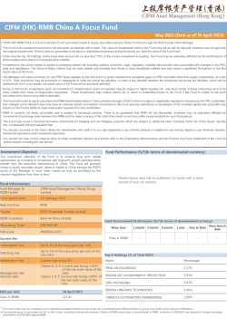
Marriage Market Matching and
Conspicuous Consumption in China
Kevin B. Grier
Daniel L. Hicks
Weici Yuan
University of Oklahoma
University of Oklahoma
University of Oklahoma
May 2015
Abstract:
Visible expenditures which convey higher socioeconomic status may help individuals
differentiate themselves in the marriage market when there is competition for
partners and imperfect information. We examine a unique dataset of automobile
purchasers in China to investigate the extent to which skewed sex ratios influence
expenditure decisions for this highly visible commodity. Using a triple difference
approach, we show that unmarried male consumers who face an unfavorable sex
ratio purchase more expensive, luxury vehicles than their married peers. Lower
income borrowers and those residing in regions with the worst sex ratios exhibit the
largest relative degree of conspicuous consumption. In addition to the direct cost of
consumption signaling, we demonstrate this behavior generates negative externalities
in the form of lower average fuel economy and higher average vehicle weight. As it
has worsened sex ratios, status competition and the associated negative repercussions
we identify represent unintended consequences of China’s one child policy.
JEL Codes: O12, E21, J12
Acknowledgements: We would like to thank Robin Grier, Joan Hicks, and Beatriz Maldonado for
helpful comments and discussions. Any errors are our own.
1. Introduction
A preference for sons, coupled with the one child-policy, has combined to generate a relative
shortage of females in China. Estimates from China’s Population Census suggests that for cohorts
born over the period 1970-2000, males have grown in share from 51% to 57% of the total
population (Qian, 2008, p1251). Estimates of the share of “missing women” in the country now
exceed 40 million women (Bulte et al., 2011). Existing research has shown that these skewed sex
ratios are producing widespread social and economic upheaval, including higher saving rates,
ballooning housing prices (Wei and Zhang, 2011; Wei et al., 2012), higher rates of bachelorhood
(Guilmoto, 2011), and reduced overall welfare (Bhaskar, 2011). Recent research also suggests that
spending on status goods appears to be growing in magnitude, even in poorer parts of rural China
(Brown et al., 2011; Chen et al., 2012).
In this paper, we investigate the extent to which skewed sex ratios influence expenditure
decisions in a broad sample of roughly 24,000 automobile transactions across China over the period
2009-2011. Using a differences in differences in differences approach, we show that unmarried male
consumers who reside in an area with an unfavorable sex ratio purchase more expensive vehicles
than their married peers. We also identify specific luxury vehicle models and confirm that the cars
purchased by these consumers are more likely to be classified as higher end models.
The pressure generated by skewed sex-ratios on individuals to consume conspicuously may
vary along a number of dimensions. We are able to explore two sources of heterogeneity in our
sample. First, we show that the estimated relationship is both larger in magnitude and more precisely
estimated among the quartile of individuals living in areas with the most highly skewed sex ratios.
Second, we find that the poorest quartile of unmarried males in our sample exhibit the largest
changes in expenditure.1 This result is consistent with a situation in which individuals of varying
income (and potentially of varying reference groups) use different sets of commodities to signal
wealth, as documented by Chai and Kaus (2012) for South African consumers. Finally, we
investigate whether this behavior generates negative externalities in the form of lower average fuel
economy and higher average vehicle weight, a factor that can significantly increase mortality in
traffic accidents (Anderson and Auffhammer, 2014). Our results suggest that consumption signaling
skews the pool of purchased automobiles to slightly lower gas mileage vehicles, but has little impact
on overall vehicle weight.
1
Our sample of car buyers is more affluent than the population at large. We explore the sample at length in Section 2.
1
The use of consumption expenditure to signal social status has attracted a great deal of
attention in the economics literature. Recent work has focused on empirically identifying
consumption visibility and exploring the determinants and motivations for signaling (Charles et al.,
2009; Heffitz, 2011). These efforts routinely classify automobiles as among the most conspicuous of
purchases and a number of papers focus specifically on vehicle purchases. For instance, Grinblatt et
al. (2008) show that Finnish consumers are directly influenced by the automobile purchases of their
nearest neighbors, particularly for recent purchases.
Positional spending has also been studied in developing countries, with research highlighting
the fact that the allocation of expenditure for this purpose has the potential to act as a poverty trap
in this setting (Banerjee and Duflo, 2007; Brown et al., 2011; Moav and Neeman, 2010, 2012; Case et
al., 2013; Kaus, 2013). These effects appear to be amplified by marriage market conditions. For
instance, Chen et al., (2012) show that relative to families with daughters, poor Chinese households
with sons undertake higher levels of social gift-giving associated with maintaining guanxi, networks
of influence in Chinese society.
Our analysis sample confers several unique advantages in this context. First, we examine
expenditure on automobiles, a ubiquitous and highly visible commodity, with a range of purchase
options, and for which signaling is often considered a major consumption motivation. Second, our
study spans consumers across all of China, both rural and urban. Finally, because the data comes
from a financial lender, our data contains information about the products purchased as well as
detailed records on the consumers themselves.
At the same time, a feature of our sample is that, because we are working with a very specific
set of consumers and consumption decisions, this may limit the generalizability of the results we
obtain. In particular, we are identifying a relationship between positional spending and marriage
market competition within a subsample of Chinese car consumers, who are affluent enough to buy a
car but both need to borrow to make their purchase and engage with this specific lender. Rates of
private car ownership in China are low but are increasing rapidly. While in 1985 the rate of
ownership was only 0.27 for every 1000 people, this rate has risen to 55 per 1000 in 2011 (Feng and
Li, 2013). Rising affluence combined with growing automobile ownership suggests that the scope
for status competition through vehicles and the effects that we observe may intensify in the future.
The extent to which our findings apply more broadly depends on the extent to which this group is
selected and to which motivations for consumption signaling could vary across other commodities,
over time, or by income level.
2
Our paper is organized as follows. Section II describes the construction of our dataset and
presents summary statistics on the sample investigated. Section III undertakes the differences in
differences analysis and discusses the implications of marriage market competition for consumption
behavior in this setting. Section IV explores the potential for heterogeneity in the estimated
relationship and examines several potential implications of consumption signaling behavior specific
to the automobile industry. Section V concludes.
2. Data
The data is constructed from three principal sources. Information on automobile
transactions and car purchasers themselves is provided by a large Chinese financial institution from
2009 through 2011. The source provides records on 24,134 individual loans, and includes borrowers
from all provinces of mainland China except Tibet. A key advantage of this data is the level of detail
contained on the vehicles purchased and on individual borrowers including information on marital
status, age, gender, education, and earnings as well as on the geographic location of purchase. We
also derive information on prefecture-level outcomes, which are obtained from both provincial
statistical yearbooks or from the National Bureau of Statistics (CEInet, 2015).
Panel A of Table 1 presents summary statistics on car buyer characteristics. One noticeable
feature is that borrowers are comparatively rich, with average annual earnings of nearly 100,000
RMB, which is over $16,000. In contrast, average income per capita is roughly 35,100 RMB
according to the National Bureau of Statistics of China, which highlights that the sample of car
purchasers is highly selected. Most purchasers are male, middle-aged, married and have received at
least a college education. Panel B provides detail on the cars purchased in the sample.2 As can be
seen from the table, over half of the cars are foreign brands and approximately one-fourth are luxury
vehicles. The average miles-per-gallon (MPG) is city/highway combined and is slightly below 30.
Panel C reports prefecture-level characteristics. The dataset contains transactions occurring
in some 292 of the 334 total prefectures in China, while we have prefecture-level economic statistics
for roughly 254 regions. Across regions with data, average income is 45,324 RMB. The mean GDP
per capita across prefectures in our sample is higher than China’s GDP per capita in 2011 (35,100
RMB), a difference which reflects the fact that more automobile purchases are undertaken by
Expenditures have been deflated to real prices using a base month of September 2010 and the official consumer price
index.
2
3
inhabitants of wealthier regions and that this value is not population weighted. 3 The overall sex ratio
is roughly 1.05 males per female across all prefectures, although this value is more skewed for
younger cohorts. Furthermore, this value masks substantial geographic heterogeneity; Figure 1
depicts the sex ratio by prefecture (measured as the ratio of males per 100 females). Although some
of the most severely imbalanced gender ratios exist in rural areas, the issue is not limited to such
areas. Overall, the sex ratio ranges from a low of 90 to a high of over 132 men per 100 women.
3. Analysis
Estimating the relationship between the level of competition in the marriage market (here
measured by the sex ratio) and positional spending (captured by the purchases of more luxurious
automobiles) is complicated by a number of factors. For example, a primary concern is that the
presence of a more skewed sex ratio may be correlated with other omitted factors such as variation
in terms of average incomes, education levels, or even male/female gender roles in a region.
We attempt to mitigate this and related sources of endogeneity through the use of a triple
differences approach. Specifically, we compare male and female car purchasers, who are and are not
married, across low and high sex ratio regions. Our identification of the effects of high sex ratio on
Chinese men’s car-purchasing preference thus relies on the interaction between gender and marital
status. In Chinese culture, the family of a groom is traditionally responsible for purchasing a house
at the time of marriage, suggesting that males may also have a stronger incentive than females at this
stage of their life to signal wealth through a range of visible expenditures (Wei et al., 2012). This
pressure has intensified with increasing competition for brides and the incentive should act on the
unmarried rather than on married men (Wei and Zhang, 2011).
For illustrative purposes, we begin our analysis with a simple triple difference mean estimate
presented in Table 2. We set the regions in the top quartile of sex ratio imbalance as the Unbalanced
group and regions in the bottom quartile as the Balanced group. 4 In the Unbalanced group,
unmarried men, on average, purchase cars that are 7025 RMB (column (5)) more expensive than
those unmarried women purchase. By contrast, for married individuals, men’s automobiles are only
811 RMB (column (6)) more expensive than married women’s purchases. The difference in
difference is 6214 RMB as is shown in the top of column (7).
The financial institution may also be more likely to make loans to individuals in richer prefectures. In order to maintain
a representative sample of Chinese consumers, we exclude those with annual incomes in excess of 250,000 RMB.
4 The sex ratios in these two groups are 107.7 and 102.5 respectively.
3
4
Next we carry out the same analysis for the Balanced sex ratio group. We find that the
difference-in-difference here is small but actually negative (-996 RMB as shown in the middle of
column 7), implying that there is no obvious car-related conspicuous consumption in this group.
Finally, our triple difference estimate is simply the difference between the two double differences:
7210 RMB, (or around $1200) which is an economically important effect.
In what follows, we run regressions that implement a regression version of this basic tripledifference approach. Equation (1) presents this triple difference estimation strategy, with all
component interactions included:
Carprice  α  β1male  β2 unmarried  β3sexratio
 β4 male * unmarried  β5 male * sexratio  β6sexratio * unmarried
(1)
 β7 male * unmarried * sexratio  θX  Z    ε
where X is a vector of borrower characteristics and Z is a vector of prefecture and province level
controls. In theory, the coefficient on the triple interaction, β7, should isolate the specific portion of
consumption expenditure undertaken by the group with the highest motivation to signal status,
unmarried males facing high levels of competition. In some specifications, we also include a set of
province fixed effects, denoted by η.
The results of estimating equation (1) are presented in Table 3 with each column (1)-(5)
adding additional controls. Column (1) estimates the triple difference with no controls. Column (2)
includes controls for borrower characteristics including age, age squared, earnings and educational
attainment, while column (3) additionally includes the prefecture characteristics listed in Table 1.
Finally, column (4) includes province fixed effects, while column (5) incorporates a control for
housing prices (for regions of the China with available data) because houses have also been
specifically shown to be a positional good in the Chinese case (Wei and Zhang, 2012). We include
controls for local housing prices only in some specifications because they dramatically limit the
sample.
In all specifications, the coefficient estimate of interest on the triple interaction term is
positive and statistically significant at the .10 level or better. The estimated impacts are economically
meaningful as well. To put the magnitude of the coefficients in perspective, the estimated coefficient
on the triple interaction in Column (5) implies that if one were to go from a prefecture in which
there is parity in the sex ratio to a prefecture with a sex ratio that is 1 standard deviation above the
mean in favor of males, then the typical car purchased by an unmarried male would be 4,285 RMB
5
more expensive. This change represents a 3.3% increase in the mean purchase price paid by this
group of consumers.
An additional concern is that several large Chinese cities such as Beijing, Guangzhou, and
Shanghai have also enacted vehicle ownership restrictions such as auctions and lotteries in an effort
to curb congestion and pollution (Feng and Li, 2013). Restrictions may alter the pool of individuals
eligible to purchase cars and may limit the scope for status competition through consumption
signaling in these regions. As a check, Appendix Table 1 demonstrates that the results we obtain are
robust to the exclusion of these areas.
Higher purchase prices could reflect numerous car characteristics, not all of which may
equally convey status. An advantage of studying automobiles is that vehicles are already classified as
standard or as luxury models both across and within producers. As an alternative approach, we
consider the likelihood an individual purchases a car which is classified as luxury. To do this we
estimate an equation as in (1), using a probit specification, with an outcome variable which is an
indicator taking the value of one for luxury automobiles. The results of this exercise are presented in
Column (6) of Table 3 and are reported as the marginal effect. Using the same comparison as in
Column (5), the estimates suggest that unmarried male consumers in prefectures one standard
deviation above the mean would be 4.8 percentage points more likely to purchase a luxury car than
those in a balanced prefecture.
While the OLS results are instructive, the use of income as a regressor in the model makes it
possible that we may have issues with heteroskedasticity.5 In fact both a general test (the White test)
and a specific test focusing on income (the Goldfeld-Quandt test) decisively reject the null of
homoscedasticity at the 0.01 level (results not shown). As a result, we re-estimate our model in Table
4 using Feasible Generalized Least Squares (FGLS) where the error variance is proportional to
income raised to an unknown exponent that we estimate in a first stage regression using the OLS
residuals. As can be seen, our coefficient of interest, the interaction of unmarried, male, and the sex
ratio is fairly constant in size across the two approaches, but estimated much more precisely using
FGLS. The estimates now exhibit significance at the .05 level or better in all five specifications. We
thus use the FGLS model approach for our subsequent analyses.
Heteroskedasticity related to scale is a classic case in the literature, and if the scale variable is also included as a
regressor in the model, the efficiency gains from using GLS can be substantial. See Baum (2006, pp. 144-147).
5
6
4. Extensions
4.1 Heterogeneous Effects
Results presented in Tables 3 and 4 suggest a highly significant conspicuous consumption
effect, where every one point increase in the sex ratio raises car spending by roughly 450 RMB for
unmarried males relative to all other types of individuals. In this subsection we consider two possible
types of heterogeneity in this relationship. The first is heterogeneity across income levels. This is
especially important in the context of conspicuous consumption where the positional goods used for
signaling may vary for different reference groups and income levels (Chai and Kaus, 2012). For
example, in our context, it is quite possible that, at very high levels of income, unmarried males use
ownership of houses or land to signal their worthiness to potential partners (as demonstrated by Wei
and Zhang, 2011) while those with lower income levels compete by signaling with relatively lower
cost commodities such as automobiles.
To investigate, we split our data in quartiles of income and estimate a separate triple
difference FGLS regression within each subgroup. These results are reported in Table 5 and strongly
suggest that the use of cars as a signaling mechanism is concentrated primarily in the lower income
quartile in our sample. Specifically, we document a highly significant average effect which is roughly
50% to 100% larger than our average effect estimated for the full sample. Estimates for the second
income quartile are small, negative and not significantly different from zero. Those for the third and
fourth income quartiles also show effects larger than our full sample estimates, but they are generally
not precisely estimated, only occasionally reaching significance at the 0.10 level.
A second possibility we investigate is that pressure for consumption signaling may vary in a
non-linear manner across regions as a function of the relative shortage of women. For example, it
may be that a one unit change in the sex ratio in highly skewed regions may not have the same effect
on the consumption pattern of unmarried males in only weakly skewed regions. It could be the case
that at relatively balanced sex ratios, the incentive to compete by conspicuous consumption may be
attenuated relative to the incentive at higher ratios. We investigate this case in Table 6 which parcels
the sample in quartiles of the sex ratio distribution. It is apparent that robust and precise estimates
only appear for the most skewed sex ratio regions.
Our sample is not large enough to split the data by both sex ratio and income quartiles at
once and still precisely estimate the model, but the results above are suggestive of the notion that is
the relatively poorest males in the regions with the most imbalanced sex ratios that heavily use car
purchases as conspicuous consumption to signal to potential marriage partners.
7
4.2 Externalities Associated with Conspicuous Consumption
A number of studies have established negative impacts of consumption signaling. This
includes diversion of expenditures away from commodities thought to have positive externalities
such as education, with particularly detrimental consequences for lower income households
(Banerjee and Duflo, 2007; Brown et al., 2011; Charles et al., 2009; Moav and Neeman, 2010, 2012;
Case et al., 2013; Kaus, 2013). Other authors have argued that collective action may make
conspicuous consumption an unproductive necessity. In other words, to the extent that everyone
within a reference group undertakes some expenditure specifically to signal status, the ultimate result
can be that individuals engage in a rat race with no net change in local distribution of status
(Hopkins & Kornienko, 2004).6 We explore a further potential impact of this behavior – that the
expenditure changes may directly generate negative externalities.
Automobiles are a commonly studied commodity thought to generate negative externalities
due to their impact on air pollution, congestion, and use of natural resources. Some of these can be
quantified and measured in a standardized form. For our sample, we compile data on average
mileage (in MPG) and weight (in lbs) of all vehicles in our data. MPG should be informative of the
impact cars have on both resource use and on pollution, as well as the vehicle’s lifetime usage cost.
Weight can generate negative externalities, both through its impact on average MPG and through its
impact on the severity of car crashes (Anderson and Auffhammer, 2014).
To get a sense for how large the impact of these externalities could be, we focus on
prefectures in the highest quartile of skewed sex ratio and estimate the FGLS regression as in Table
6.7 As can be seen from the Table 7, cars purchased by unmarried males in the most skewed regions
exhibit both lower fuel economy and higher weight. The MPG effect is rather sizeable, with a one
unit increase in the sex ratio among the most skewed sex ratio regions being associated with a
reduction in fuel efficiency in the range of 0.30 to 0.47 MPG. This suggests that consumption
signaling in this setting may indeed be exacerbating this class of existing negative externalities
associated with automobiles. Interestingly, the impact of vehicle weight is not economically
meaningful in size with these vehicles being only a few pounds heavier per unit change in the sex
In such a world, there exists a pareto-improvement in which one could reallocate everyone’s expenditure away from
positional commodities in favor of others which may be desirable on other grounds, but doing so unilaterally is not
individually rational, as failing to signal alone would net a relative fall in status.
7 Estimates obtained from regressions utilizing the full sample are roughly one fourth to one half of those for this group
in magnitude and are generally less precisely estimated.
6
8
ratio.8 As can be seen in Panel B of Table 1, the standard deviation of weight is pretty low as well,
suggesting that cars purchased in China are relatively homogenous in size.
5. Conclusion
Using a novel dataset on borrowers in China, we have shown that the increasingly skewed
sex ratios in many parts of the country are creating incentives for unmarried men to significantly
alter their automobile consumption habits in ways that appear competitive in nature. The effects that
we observe are strongest in the quartile of regions with the most unbalanced sex ratios, suggesting
that positional spending may yet worsen if the sex ratio continues to deteriorate.
We further demonstrate that the largest expenditure reallocations occur among the poorest
quartile of borrowers in our sample. This evidence supports the hypothesis that the range of
commodities used to jockey for social status varies across individuals in different portions of the
income distribution (or among those facing different peer groups). Beyond the direct social
inefficiency that status competition represents, we demonstrate that this behavior also leads to
consumption of vehicles with lower vehicle fuel efficiency. Thus, to the extent that China’s one child
policy has generated incentives which further skewed sex ratios, it may also have exacerbated social
status competition. In many areas of the country, unmarried men now appear to compete in a zerosum game of consumption signaling, one which is capable of generating large negative externalities.
Given that there is little reason to suspect that growth in the rate of car ownership in China will
slow, conspicuous consumption may become even more important and generate greater aggregate
distortions as time passes.
8
This suggests that it is possible to signal status through vehicle quality without requiring larger cars to do so.
9
References
Anderson, Michael L., and Maximilian Auffhammer. (2014). "Pounds that kill: the external costs of
vehicle weight." The Review of Economic Studies Vol. 81(2): 535-571.
Banerjee, Abhijit V., and Esther Duflo. (2007). "The Economic Lives of the Poor." Journal of
Economic Perspectives, 21(1): 141-168.
Baum, Christopher F. (2006). An Introduction to Modern Econometrics Using Stata. Stata Press,
College Station, Texas.
Bhaskar, V. (2011). "Sex selection and gender balance." American Economic Journal: Microeconomics: Vol.
3(1), 214-244.
Brown, Philip H., Erwin Bulte, and Xiaobo Zhang. (2011). "Positional spending and status seeking
in rural China." Journal of Development Economics 96.1: 139-149.
Bulte, Erwin, Nico Heerink, and Xiaobo Zhang. (2011). "China's One‐Child Policy and ‘the Mystery
of Missing Women’: Ethnic Minorities and Male‐Biased Sex Ratios." Oxford Bulletin of Economics
and Statistics 73.1: 21-39.
Case, Anne, Anu Garrib, Alicia Menendez, and Analia Olgiati. (2013). "Paying the piper: The high
cost of funerals in South Africa." Economic Development and Cultural Change Vol. 62(1): 1-20.
Chai, Andreas and Wolfhard Kaus. (2012). “Signalling to whom? Conspicuous spending and the
local density of the social group income distribution.” Working Paper No. 1218. Papers on
Economics and Evolution.
Charles, Kerwin Kofi, Erik Hurst, and Nikolai Roussanov. (2009). "Conspicuous Consumption and
Race." The Quarterly Journal of Economics Vol. 124(2): 425-467.
Chen, Xi, Ravi Kanbur, and Xiaobo Zhang. (2012). "Peer effects, risk pooling, and status seeking:
What explains gift spending escalation in rural China?." Working Paper
Feng, Suwei, and Qiang Li. (2013) "Car Ownership Control in Chinese Mega Cities: Shanghai,
Beijing and Guangzhou." Journeys, September: 40-49
Grinblatt, Mark, Matti Keloharju, and Seppo Ikäheimo. (2008). "Social influence and consumption:
Evidence from the automobile purchases of neighbors." The Review of Economics and Statistics, Vol.
90(4): 735-753.
Guilmoto, Christophe Z. (2012). "Skewed sex ratios at birth and future marriage squeeze in China
and India, 2005–2100." Demography 49.1: 77-100.
10
Heffetz, Ori. (2011). “A test of conspicuous consumption: Visibility and income elasticities.” Review
of Economics and Statistics, 93(4): 1101-1117.
Hopkins, Ed, and Tatiana Kornienko. (2004). "Running to keep in the same place: consumer choice
as a game of status." American Economic Review Vol. 94(4): 1085-1107.
Kaus, Wolfhard. (2013). “Conspicuous consumption and “race”: Evidence from South Africa.”
Journal of Development Economics, Vol. 100(1): 63-73.
Moav, Omer, and Zvika Neeman. (2010). "Status and poverty." Journal of the European Economic
Association Vol. 8(2‐3): 413-420.
Moav, Omer and Zvika Neeman. (2012). "Saving Rates and Poverty: The Role of Conspicuous
Consumption and Human Capital." The Economic Journal , Vol. 122(563): 933-956.
Qian, Nancy. (2008) "Missing Women and the Price of Tea in China: The Effect of Sex-Specific
Earnings on Sex Imbalance." The Quarterly Journal of Economics, Vol. 123(3): 1251-1285.
Wei, Shang-Jin, and Xiaobo Zhang. (2011). "The Competitive Saving Motive: Evidence from Rising
Sex Ratios and Savings Rates in China." Journal of Political Economy Vol. 119(3): 511-564.
Wei, Shang-Jin, Xiaobo Zhang, and Yin Liu. (2012) “Status competition and housing prices. National
Bureau of Economic Research Working Paper No. w18000.
11
Figure 1: Sex Ratios by Prefecture
Table 1: Summary Statistics
Panel A: Borrower Characteristics
Age
Male
Earnings
Married
Educational Attainment
Illiterate
Elementary
High School
College
Graduate
Panel B: Car Characteristics
Purchase Price
Foreign
Luxury Make
Fuel Efficiency (Combined mpg)
Vehicle Weight (lbs)
Panel C: Prefecture Characteristics
Sex Ratio (Male/Female*100)
Income (GDP per capita)
Population (10,000)
Mean House Price in Jan 2010 (per square meters)
Paved Road Area (per capita)
Buses (Per 10,000 people)
Taxis (Per 10,000 people)
Obs
24,133
24,133
24,133
24,133
Mean
35.62
0.75
98,027
0.84
Std. Dev.
7.91
0.43
51,608
0.37
24,133
24,133
24,133
24,133
24,133
0.00
0.10
0.30
0.59
0.01
0.02
0.30
0.46
0.49
0.11
24,133
24,133
24,133
24,133
24,133
131,071
0.56
0.24
29.35
1,360
46,724
0.50
0.43
3.31
154
292
254
254
97
253
254
254
105.28
45,324
135.40
7,037
10.87
7.72
22.26
4.22
29,611
152.47
4,556
7.29
7.75
18.20
Notes: Pooled sample spanning 2009-2011. Expenditures are deflated to real 2010 RMB prices using the
CPI. Sample excludes individuals earning in excess of 250,000 RMB per year.
Source: Panel A and B: Author's calculations using vehicle loan data detailed in Section 4; MPG
information obtained from the Ministry of Industry and Information Technology of China (2014). Panel C:
Most variables are obtained from China Economic Information Network (CEInet) Statistics Database. Sex
ratios are derived from the provincial statistical yearbooks (2011) and mean house prices are obtained from
www.elivecity.cn.
Table 2: Mean Differences in Differences of Car Price
by Gender, Marital Status, and Sex Ratio
Unmarried
Married
Unmarried
Married
Unmarried
Married
Difference
in
Difference
Sex Ratio
(1)
(2)
(3)
(4)
(5)=(1)-(3)
(6)=(2)-(4)
(7)=(5)-(6)
Unbalanced
131,084
(47570)
119,417
(38078)
142,438
(50763)
130,114
(44786)
124,059
(41981)
115,302
(35841)
141,627
(53044)
125,003
(43586)
7,025
811
6,214
4,115
5,111
-996
Men
Balanced
Women
Diff-in-Diff-in-Diff
Notes: Sources and sample as described in Table 1. Standard deviation in parenthsis.
Difference
7,210
Table 3: The Impact of the Sex Ratio on the Automobile
Purchase Price of Unmarried Males in China
Male
Unmarried
Sex Ratio
Unmarried*Sexratio
Unmarried*Male
Sexratio*Male
Sexratio*Male*Unmarried
Borrower Characteristics
Prefecture Characteristics
Province Fixed Effects
Housing Price Controls
Mean of Dependant Variable
Number of Observations
R2
Dependent Variable: Automobile Sales Price
1
2
3
36,586.87**
22,608.06
23,510.13
(16,194.21)
(16,433.08)
(16,586.20)
34,481.83**
38,869.18***
37,044.48***
(15,212.31)
(14,662.75)
(14,334.04)
1,031.63***
849.15***
881.22***
(137.28)
(147.28)
(196.07)
-432.94***
-497.56***
-479.39***
(144.91)
(134.61)
(132.71)
-42,378.37**
-42,168.00**
-36,111.73*
(17,829.39)
(19,622.71)
(19,243.25)
-322.14**
-285.94*
-294.39*
(147.77)
(148.89)
(150.44)
401.46**
505.32***
443.55**
(172.08)
(183.77)
(180.79)
4
24,749.06*
(13,530.58)
36,511.51*
(20,165.34)
600.83***
(126.05)
-473.88**
(193.59)
-37,093.93
(26,863.08)
-304.69**
(129.99)
451.32*
(258.10)
5
29,546.31**
(14,436.89)
36,289.46*
(20,253.01)
369.38**
(149.31)
-469.93**
(194.83)
-40,759.97
(27,978.82)
-341.41**
(139.07)
480.80*
(269.67)
Probit: Luxury
6
0.291***
(0.088)
0.406**
(0.206)
0.004**
(0.001)
-0.004***
(0.001)
-0.247***
(0.051)
-0.004***
(0.001)
0.005***
(0.002)
N
N
N
N
Y
N
N
N
Y
Y
N
N
Y
Y
Y
N
Y
Y
Y
Y
Y
Y
Y
Y
130,771
24,133
0.017
130,771
24,133
0.143
130,806
23,520
0.144
130,806
23,520
0.150
128,869
14,929
0.156
0.239
14,929
0.105
Note: Sources and sample as described in Table 1. Borrower characteristics include age, age squared, earnings, and dummies for education level.
Prefecture characteristics include income per capita, population, paved road area, buses, and taxis per capita. Standard errors are clustered at the
province level in specifications (1)-(3) and reported in parenthesis, while columns (4) and (5) report Huber-White robust standard errors in
parenthesis. Column (6) reports marginal effects from a probit regression with a dependent variable of an indicator for luxury car status.
*** p<0.01, ** p<0.05, * p<0.1
Table 4: FGLS Estimates (Variance as a Function of Earnings)
Male
Unmarried
Sex Ratio
Unmarried*Sexratio
Unmarried*Male
Sexratio*Male
Sexratio*Male*Unmarried
Borrower Characteristics
Prefecture Characteristics
Province Fixed Effects
Housing Price Controls
Mean of Dependant Variable
Number of Observations
R2
Dependent Variable: Automobile Sales Price
1
2
3
34,107.68**
17,855.65
17,966.41
(15,620.13)
(14,978.61)
(14,971.25)
32,572.44**
34,448.65**
31,942.09**
(15,168.15)
(14,660.48)
(13,927.77)
997.76***
786.94***
811.81***
(134.73)
(146.99)
(186.80)
-413.07***
-453.02***
-428.42***
(144.78)
(135.53)
(129.54)
-42,692.22**
-41,587.42**
-37,304.11*
(17,202.17)
(18,340.38)
(18,947.05)
-301.05**
-241.49*
-242.67*
(142.83)
(136.35)
(136.29)
405.43**
497.73***
454.43**
(166.50)
(171.84)
(178.63)
4
19,163.70
(14,766.65)
31,007.41**
(13,433.41)
564.03**
(238.57)
-418.67***
(125.18)
-36,907.21*
(18,983.67)
-252.89*
(134.19)
448.63**
(180.23)
5
23,896.85*
(11,976.82)
30,952.79**
(13,353.83)
295.41*
(171.11)
-415.72***
(123.11)
-37,159.15**
(16,071.10)
-289.10**
(105.18)
444.43***
(145.43)
N
N
N
N
Y
N
N
N
Y
Y
N
N
Y
Y
Y
N
Y
Y
Y
Y
130,771
24,133
0.017
130,771
24,133
0.143
130,806
23,520
0.144
130,806
23,520
0.150
128,869
14,929
0.156
Note: Sources, sample, and controls as described in Table 3. Standard errors are clustered at the province level in specifications
(1)-(3) and reported in parenthesis, while columns (4) and (5) report Huber-White robust standard errors in parenthesis.
*** p<0.01, ** p<0.05, * p<0.1
Table 5: Exploring Earnings Heterogeneity
1st Quartile
2nd Quartile
3rd Quartile
4th Quartile (Highest Earners)
Borrower Characteristics
Prefecture Characteristics
Province Fixed Effects
Housing Price Controls
Dependent Variable: Automobile Sales Price
1
2
3
1,033***
920***
794***
(251)
(255)
(241)
-283
-239
-149
(322)
(326)
(268)
710
754*
658
(466)
(404)
(425)
499
550
511
(609)
(513)
(512)
N
N
N
N
Y
N
N
N
Y
Y
N
N
4
769***
(260)
-94
(266)
739*
(426)
479
(515)
5
717**
(277)
-71
(204)
487
(288)
954*
(538)
Y
Y
Y
N
Y
Y
Y
Y
Note: Sources, sample, and controls as described in Table 3. FGLS estimates of the triple interaction coefficient from Table 4.
Overall sample is 24,133 split into quartiles. Standard errors are clustered at the province level in specifications (1)-(3) and
reported in parenthesis, while columns (4) and (5) report Huber-White robust standard errors in parenthesis.
*** p<0.01, ** p<0.05, * p<0.1
Table 6: Exploring Regional Sex Ratio Heterogeneity
1st Quartile
2nd Quartile
3rd Quartile
4th Quartile (Most Skewed)
Borrower Characteristics
Prefecture Characteristics
Province Fixed Effects
Housing Price Controls
Dependent Variable: Automobile Sales Price
1
2
3
-368
305
330
(542)
(440)
(418)
2,098
5,442
6,481*
(3,640)
(3,526)
(3,487)
282
-2,536
-1,491
(4,661)
(2,556)
(2,504)
724***
403**
374**
(189)
(150)
(161)
N
N
N
N
Y
N
N
N
Y
Y
N
N
4
377
(364)
6,654*
(3,465)
-1,016
(2,852)
353**
(147)
5
651
(490)
5,015
(2,990)
-4,405
(2,950)
280
(210)
Y
Y
Y
N
Y
Y
Y
Y
Note: Sources, sample, and controls as described in Table 3. FGLS estimates of the triple interaction coefficient from Table 4.
Overall sample is 24,133 split into quartiles. Standard errors are clustered at the province level in specifications (1)-(3) and
reported in parenthesis, while columns (4) and (5) report Huber-White robust standard errors in parenthesis.
*** p<0.01, ** p<0.05, * p<0.1
Table 7: Externalities Associated with Luxury Purchases
Dependent Variable
Fuel Efficiency
Vehicle Weight
Borrower Characteristics
Prefecture Characteristics
Province Fixed Effects
Housing Price Controls
1
-0.047***
(0.014)
2.44***
(0.67)
2
-0.038***
(0.012)
1.67**
(0.60)
3
-0.030***
(0.010)
1.54**
(0.60)
4
-0.030***
(0.010)
1.55**
(0.61)
5
-0.032**
(0.013)
1.76***
(0.54)
N
N
N
N
Y
N
N
N
Y
Y
N
N
Y
Y
Y
N
Y
Y
Y
Y
Note: Sources, sample, and controls as described in Table 4. FGLS estimates of the triple interaction coefficient from Table 6
for the fourth quartile of sex ratio. Samples range from 5,973 to 5,703 observations except for column (6) which has 2,337
observations. Standard errors are clustered at the province level in specifications (1)-(3) and reported in parenthesis, while
columns (4) and (5) report Huber-White robust standard errors in parenthesis.
*** p<0.01, ** p<0.05, * p<0.1
Appendix Table 1: Excluding Cities with Ownership Restrictions
Male
Unmarried
Sex Ratio
Unmarried*Sexratio
Unmarried*Male
Sexratio*Male
Sexratio*Male*Unmarried
Borrower Characteristics
Prefecture Characteristics
Province Fixed Effects
Housing Price Controls
Mean of Dependant Variable
Number of Observations
R2
Dependent Variable: Automobile Sales Price
1
2
3
36,863.57**
19,449.57
19,755.79
(15,905.76)
(15,815.61)
(15,904.49)
35,602.73**
37,400.47**
34,887.62**
(14,375.00)
(15,525.67)
(14,767.52)
1,021.11***
795.33***
822.79***
(139.86)
(154.33)
(199.81)
-440.57***
-479.42***
-454.68***
(136.90)
(143.60)
(137.31)
-41,921.58**
-40,664.60**
-37,062.16*
(17,755.54)
(19,185.87)
(20,038.23)
-325.75**
-256.32*
-259.14*
(144.68)
(143.84)
(144.78)
398.55**
489.82**
452.68**
(171.29)
(179.28)
(188.39)
4
21,077.00
(15,675.42)
33,604.08**
(14,115.36)
579.98**
(242.01)
-442.06***
(131.49)
-36,903.49*
(19,975.29)
-270.43*
(142.46)
449.11**
(188.93)
5
26,956.20**
(12,839.15)
34,271.76**
(14,243.03)
319.05*
(171.96)
-445.03***
(131.59)
-37,800.37**
(17,537.81)
-316.61***
(113.28)
450.79***
(157.97)
N
N
N
N
Y
N
N
N
Y
Y
N
N
Y
Y
Y
N
Y
Y
Y
Y
130,946
23,339
0.017
130,946
23,339
0.135
130,987
22,726
0.137
130,987
22,726
0.143
129,052
14,135
0.149
Note: FGLS estimates. Sources, sample, and controls as described in Table 4. Standard errors are clustered at the province level in
specifications (1)-(3) and reported in parenthesis, while columns (4) and (5) report Huber-White robust standard errors in
parenthesis.
*** p<0.01, ** p<0.05, * p<0.1