1. No category

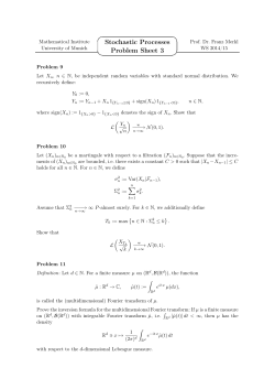
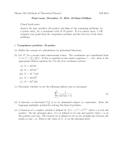
4.5 Fourier and Laplace Transforms
7.
267
(a) Consider the mapping w = z 3 . When we encircle the origin in the z
plane one time, how many times do we encircle the origin in the w
plane? Explain why this agrees with the Argument Principle.
(b) Suppose we consider w = z 3 + a2 z 2 + a1 z + a0 for three constants
a0 , a1 , a2 . If we encircle the origin in the z plane once on a very large
circle, how many times do we encircle the w plane?
(c) Suppose we have a mapping w = f (z) where f (z) is analytic inside
and on a simple closed contour C in the z plane. Let us define C˜ as the
(nonsimple) image in the w plane of the contour C in the z plane. If we
deduce that it encloses the origin (w = 0) N times, and encloses the
point (w = 1) M times, what is the change in arg w over the contour
˜ If we had a computer available, what algorithm should be designed
C?
(if it is at all possible) to determine the change in the argument?
∗
4.5 Fourier and Laplace Transforms
One of the most valuable tools in mathematics, physics, and engineering is
making use of the properties a function takes on in a so-called transform (or
dual) space. In suitable function spaces, defined below, the Fourier transform
pair is given by the following relations:
! ∞
1
ikx
ˆ
f (x) =
F(k)e
dk
(4.5.1)
2π −∞
! ∞
ˆF(k) =
f (x)e−ikx d x
(4.5.2)
−∞
ˆ
F(k)
is called the Fourier transform of f (x). The integral in Eq. (4.5.1) is
referred to as the inverse Fourier transform. In mathematics, the study
of Fourier transforms is central in fields like harmonic analysis. In physics
and engineering, applications of Fourier transforms are crucial, for example,
in the study of quantum mechanics, wave propagation, and signal processing.
In this section we introduce the basic notions and give a heuristic derivation
of Eqs. (4.5.1)–(4.5.2). In the next section we apply these concepts to solve
some of the classical partial differential equations.
In what follows we make some general remarks about the relevant function
ˆ
spaces for f (x) and F(k).
However, in our calculations we will apply complex
variable techniques and will not use any deep knowledge of function spaces.
ˆ
Relations (4.5.1)–(4.5.2) always hold if f (x) ∈ L 2 and F(k)
∈ L 2 , where
f ∈ L 2 refers to the function space of square integrable functions
"! ∞
#1/2
2
∥ f ∥2 =
| f | (x) d x
<∞
(4.5.3)
−∞
268
4 Residue Calculus and Applications of Contour Integration
In those cases where f (x) and f ′ (x) are continuous everywhere apart from
a finite number of points for which f (x) has integrable and bounded discontinuities (such a function f (x) is said to be piecewise smooth), it turns out
that at each point of discontinuity, call it x0 , the integral given by Eq. (4.5.1)
converges to the mean: limϵ→0+ 12 [ f (x0 + ϵ) + f (x0 − ϵ)]. At points where
f (x) is continuous, the integral (4.5.1) converges to f (x).
There are other function spaces for which Eqs. (4.5.1)–(4.5.2) hold. If
f (x)
∈ L 1 , the space of absolutely integrable functions (functions f satisfy!∞
ˆ
ing −∞ | f (x)| d x < ∞), then F(k)
tends to zero for |k| → ∞ and belongs to
a certain function space of functions decaying at infinity (sometimes referred to
as bounded mean oscillations (BMO)). Conversely, if we start with a suitably
ˆ
decaying function F(k)
(i.e., in BMO), then f (x) ∈ L 1 . In a sense, purely
from a symmetry point of view, such function spaces may seem less natural
ˆ
than when f (x), F(k)
are both in L 2 for Eqs. (4.5.1)–(4.5.2) to be valid. Nevertheless, in some applications f (x) ∈ L 1 and not L 2 . Applications sometimes
require the use of Fourier transforms in spaces for which no general theory
applies, but nevertheless, specific results can be attained. It is outside the scope
of this text to examine L p ( p = 1, 2, . . .) function spaces where the general
results pertaining to Eqs. (4.5.1)–(4.5.2) can be proven. Interested readers can
find such a discussion in various books on complex or Fourier analysis, such as
Rudin (1966). Unless otherwise specified, we shall assume that our function
f (x) ∈ L 1 ∩ L 2 , that is, f (x) is both absolutely and square integrable. It
follows that
" ∞
ˆ
| F(k)| ≤ ∥ f ∥1 =
| f (x)| d x
and
−∞
1
ˆ 2 = ∥ f ∥2
√ ∥ F∥
2π
The first relationship follows directly. The second is established later in this
section. In those cases for which f (x) is piecewise smooth, an elementary
though tedious proof of Eqs. (4.5.1)–(4.5.2) can be constructed by suitably
breaking up the interval (−∞, ∞) and using standard results of integration
(Titchmarsch, 1948).
Statements analogous to Eqs. (4.5.1)–(4.5.2) hold for functions on finite
intervals (−L , L), which may be extended as periodic functions of period 2L:
f (x) =
1
Fˆ n =
2L
∞
#
Fˆ n einπ x/L
(4.5.4)
f (x) e−inπ x/L d x
(4.5.5)
n=−∞
"
L
−L
4.5 Fourier and Laplace Transforms
269
The values Fˆ n are called the Fourier coefficients of the Fourier series representation of the function f (x) given by Eq. (4.5.4).
A simple example of how Fourier transforms may be calculated is afforded
by the following.
Example 4.5.1 Let a > 0, b > 0, and f (x) be given by
! −ax
e
x >0
f (x) =
bx
e
x <0
ˆ
Then, from Eq. (4.5.2), we may compute F(k)
to be
" ∞
" 0
−ax−ikx
ˆF(k) =
e
dx +
ebx−ikx d x
0
−∞
1
1
+
(4.5.6)
a + ik
b − ik
The inversion (i.e., reconstruction of f (x)) via Eq. (4.5.1) is ascertained by
calculating the appropriate contour integrals. In this case we use closed semicircles in the upper (x > 0) and lower (x < 0) half k-planes. The inversion
can be done either by combining the two terms in Eq. (4.5.6) or by noting that
⎧ −ax
" ∞ ikx
x >0
⎨e
1
e
dk = 1/2 x = 0
⎩
2π −∞ a + ik
0
x <0
=
and
1
2π
"
∞
−∞
⎧
⎨0
e
dk = 1/2
⎩ bx
b − ik
e
ikx
x >0
x =0
x <0
The values at x = 0 take into account
both the pole and the principal value
&
1
dk
contribution at infinity; that is, 2π C R a+ik = 1/2 where on C R : k = R eiθ ,
0 ≤ θ ≤ π . Thus Eq. (4.5.1) gives convergence to the mean value at x = 0:
1
+ 12 = 1 = (limx→0+ f (x) + limx→0− f (x))/2.
2
A function that will lead us to a useful result is the following:
⎧
⎨ 1 |x| < ϵ
#(x; ϵ) = 2ϵ
⎩
0
|x| > ϵ
(4.5.7)
Its Fourier transform is given by
1
ˆ
#(k;
ϵ) =
2ϵ
"
ϵ
−ϵ
e−ikx d x =
sin kϵ
kϵ
(4.5.8)
270
4 Residue Calculus and Applications of Contour Integration
Certainly, !(x; ϵ) is both absolutely and square integrable; so it is in L 1 ∩ L 2 ,
ˆ
and !(k;
ϵ) is in L 2 . It is natural to ask what happens as ϵ → 0. The function
defined by Eq. (4.5.7) tends, as ϵ → 0, to a novel “function” called the Dirac
delta function, denoted by δ(x) and having the following properties:
δ(x) = lim !(x; ϵ)
(4.5.9)
!
(4.5.10)
ϵ→0
!
∞
−∞
δ(x − x0 )d x = lim
ϵ→0
!
∞
−∞
x=x0 +ϵ
x=x0 −ϵ
δ(x − x0 )d x = 1
δ(x − x0 ) f (x) d x = f (x0 )
(4.5.11)
where f (x) is continuous. Equations (4.5.10)–(4.5.11) can be ascertained by
using the limit definitions (4.5.7) and (4.5.9). The function defined in Eq. (4.5.9)
is often called a unit impulse “function”; it has an arbitrarily large value concentrated at the origin, whose integral is unity. The delta function, δ(x), is not
a mathematical function in the conventional sense, as it has an arbitrarily large
value at the origin. Nevertheless, there is a rigorous mathematical framework in
which these new functions – called distributions – can be analyzed. Interested
readers can find such a discussion in, for example, Lighthill (1959). For our
purposes the device of the limit process ϵ → 0 is sufficient. We also note that
Eq. (4.5.7) is not the only valid representation of a delta function; for example,
others are given by
"
#
1 −x 2 /ϵ
δ(x) = lim √ e
(4.5.12a)
ϵ→0
πϵ
"
#
ϵ
δ(x) = lim
(4.5.12b)
ϵ→0 π(ϵ 2 + x 2 )
It should be noted that, formally speaking, the Fourier transform of a delta
function is given by
! ∞
ˆ
δ(k)
=
δ(x)e−ikx d x = 1
(4.5.13)
−∞
It does not vanish as |k| → ∞; indeed, it is a constant (unity; note that δ(x)
is not L 1 ). Similarly, it turns out from the theory of distributions (motivated
by the inverse Fourier transform), that the following alternative definition of a
delta function holds:
! ∞
1
ikx
ˆ
δ(x) =
dk
δ(k)e
2π −∞
! ∞
1
=
eikx dk
(4.5.14)
2π −∞
271
4.5 Fourier and Laplace Transforms
Formula (4.5.14) allows us a simple (but formal) way to verify Eqs. (4.5.1)–
(4.5.2). Namely, by using Eqs. (4.5.1)–(4.5.2) and assuming that interchanging
integrals is valid, we have
1
f (x) =
2π
!
∞
dk e
ikx
−∞
"!
∞
′
′
d x f (x ) e
−∞
−ikx ′
"
#
! ∞
1
ik(x−x ′ )
=
d x f (x )
dk e
2π −∞
−∞
!
=
∞
!
′
∞
−∞
#
′
d x ′ f (x ′ )δ(x − x ′ )
(4.5.15)
In what follows, the Fourier transform of derivatives will be needed. The
Fourier transform of a derivative is readily obtained via integration by parts.
Fˆ 1 (k) ≡
!
=
$
∞
f ′ (x) e−ikx d x
−∞
%∞
f (x) e−ikx −∞
+ ik
!
∞
f (x) e−ikx d x
−∞
ˆ
= ik F(k)
(4.5.16a)
and by repeated integration by parts
Fˆ n (k) =
!
∞
−∞
ˆ
f (n) (x)e−ikx d x = (ik)n F(k)
(4.5.16b)
Formulae (4.5.16a,b) will be useful when we examine solutions of differential
equations by transform methods.
It is natural to ask what is the Fourier transform of a product. The result is
called the convolution product; it is not the product of the Fourier transforms.
We can readily derive this formula. We use two transform pairs: one for a
function f (x) (Eqs. (4.5.1)–(4.5.2)) and another for a function g(x), replacing
ˆ
ˆ
f (x) and F(k)
in Eqs. (4.5.1)–(4.5.2) by g(x) and G(k),
respectively. We
define the convolution product,
! ∞
! ∞
′
′
′
( f ∗ g)(x) =
f (x − x )g(x ) d x =
f (x ′ )g(x − x ′ ) d x ′ .
−∞
−∞
(The latter equality follows by renaming variables.) We take the Fourier transform of ( f ∗ g)(x) and interchange integrals (allowed since both f and g are
272
4 Residue Calculus and Applications of Contour Integration
absolutely integrable) to find
!
∞
−∞
( f ∗ g)(x)e
−ikx
dx =
=
!
∞
dx
−∞
!
∞
"!
∞
−∞
′ ikx ′
dx e
′
′
f (x − x )g(x )d x
!
′
g(x )
−∞
∞
−∞
ˆ G(k).
ˆ
= F(k)
′
#
e−ikx
′
d xe−ik(x−x ) f (x − x ′ )
Hence, by taking the inverse transform of this result,
! ∞
! ∞
1
ikx ˆ
ˆ
e F(k)G(k) dk =
g(x ′ ) f (x − x ′ ) d x ′
2π −∞
−∞
! ∞
=
g(x − x ′ ) f (x ′ )d x ′ .
(4.5.17)
(4.5.18)
−∞
The latter equality is accomplished by renaming the integration variables. Note
ˆ
that if f (x) = δ(x − x ′ ), then F(k)
= 1, and
Eq. (4.5.18) reduces to the known
$∞
1
ikx
ˆ
transform pair for g(x), that is, g(x) = 2π −∞ G(k)e
dk.
A special case of Eq. (4.5.18) is the so-called Parseval formula, obtained
by taking g(x) = f (−x), where f (x) is the complex conjugate of f (x), and
evaluating Eq. (4.5.17) at x = 0:
!
∞
−∞
1
f (x) f (x) d x =
2π
!
∞
ˆ G(k)
ˆ
F(k)
dk.
−∞
ˆ
Function G(k)
is now the Fourier transform of f (−x):
ˆ
G(k)
=
=
!
∞
e
−ikx
−∞
"!
∞
−∞
f (−x) d x =
e−ikx
f (x) d x
#
!
∞
eikx f (x) d x
−∞
ˆ
= ( F(k))
Hence we have the Parseval formula:
!
! ∞
%
%
1
% F(k)
ˆ %2 dk
| f | (x) d x =
(4.5.19)
2π −∞
−∞
$∞
In some applications,$ −∞ | f |2 (x) d x refers to the energy of a signal. Fre∞
2
ˆ
dk which is really measured (it is somequently it is the term −∞ | F(k)|
times referred to as the power spectrum), which then gives the energy as per
Eq. (4.5.19).
∞
2
4.5 Fourier and Laplace Transforms
273
In those cases where we have f (x) being an even or odd function, then
the Fourier transform pair reduces to the so-called cosine transform or sine
ˆ
transform pair. Because f (x) being even/odd in x means that F(k)
will be
even or odd in k, the pair (4.5.1)–(4.5.2) reduces
about semiinfinite
! ∞ to statements
2
2
functions in the space
! ∞L on (0, ∞) (i.e., 0 | f (x)| d x < ∞) or in the space
1
L on (0, ∞) (i.e., 0 | f (x)| d x < ∞). For even functions, f (x) = f (−x),
the following definitions
√
1
ˆ
f (x) = √ f c (x),
F(k)
= 2 Fˆ c (k)
(4.5.20)
2
ˆ
(or more generally F(k)
= a Fˆ c (k), f (x) = b f c (x), a = 2b, b ̸= 0) yield the
Fourier cosine transform pair
"
2 ∞ ˆ
f c (x) =
Fc (k) cos kx dk
(4.5.21)
π 0
" ∞
Fˆ c (k) =
f c (x) cos kx d x
(4.5.22)
0
For odd functions, f (x) = − f (−x), the definitions
√
1
ˆ
f (x) = √ f s (x),
F(k)
= − 2i Fˆ s (k)
2
yield the Fourier sine transform pair
"
2 ∞ ˆ
f s (x) =
Fs (k) sin kx dk
π 0
" ∞
ˆFs (k) =
f s (x) sin kx d x
(4.5.23)
(4.5.24)
0
Obtaining the Fourier sine or cosine transform of a derivative employs integration by parts; for example
" ∞
ˆFc,1 (k) =
f ′ (x) cos kx dk
0
=[
f (x) cos kx]∞
0
and
Fˆ s,1 (k) =
"
=[
∞
+k
"
∞
f (x) sin kx dk = k Fˆ s (k) − f (0) (4.5.25)
0
f ′ (x) sin kx dk
0
f (x) sin kx]∞
0
−k
"
0
∞
f (x) cos kx dk = −k Fˆ c (k) (4.5.26)
are formulae for the first derivative. Similar results obtain for higher derivatives.
274
4 Residue Calculus and Applications of Contour Integration
It turns out to be useful to extend the notion of Fourier transforms. One way
to do this is to consider functions that have support only on a semi-interval.
We take f (x) = 0 on x < 0 and replace f (x) by e−cx f (x)(c > 0) for
ˆ
x > 0. Then Eqs. (4.5.1)–(4.5.2) satisfy, using F(k)
from Eq. (4.5.2) in
Eq. (4.5.1):
e
−cx
1
f (x) =
2π
!
∞
dk e
ikx
"!
∞
e
−ikx ′ −cx ′
e
−(c+ik)x ′
e
′
f (x ) d x
0
−∞
′
#
hence
1
f (x) =
2π
!
∞
dk e
(c+ik)x
"!
∞
′
f (x ) d x
0
−∞
′
#
Within the above integrals we define s = c + ik, where c is a fixed real
constant, and make the indicated redefinition of the limits of integration to
obtain
1
f (x) =
2πi
!
c+i∞
ds e
c−i∞
sx
$!
∞
e
−sx ′
′
f (x ) d x
0
′
%
or, in a form analogous to Eqs. (4.5.1)–(4.5.2):
! c+i∞
1
sx
ˆ
f (x) =
F(s)e
ds
2πi c−i∞
! ∞
ˆ
F(s)
=
f (x)e−sx d x
(4.5.27)
(4.5.28)
0
ˆ
Formulae (4.5.27)–(4.5.28) are referred to as the Laplace transform ( F(s))
and the inverse Laplace transform of a function ( f (x)), respectively. The usual
function space for f (x) in the Laplace transform (analogous to L 1 ∩ L 2 for
f (x) in Eq. (4.5.1)) are those functions satisfying:
!
0
∞
e−cx | f (x)| d x < ∞.
(4.5.29)
Note Re s = c in Eqs. (4.5.27)–(4.5.28). If Eq. (4.5.29) holds for some c > 0,
then f (x) is said to be of exponential order.
The integral (4.5.27) is generally carried out by contour integration. The
contour from c − i∞ to c + i∞ is referred to as the Bromwich contour, and
c is taken to the right of all singularities in order to insure (4.5.29). Closing the
contour to the right will yield f (x) = 0 for x < 0.
275
4.5 Fourier and Laplace Transforms
c+iR
iω
CR
2
-CR
1
-i ω
c-iR
Fig. 4.5.1. Bromwich contour, Example 4.5.2
We give two examples.
ˆ
Example 4.5.2 Evaluate the inverse Laplace transform of F(s)
=
ω > 0. See Figure 4.5.1.
1
f (x) =
2πi
!
c+i∞
c−i∞
1
,
s 2 +ω2
with
esx
ds
s 2 + w2
For x < 0 we close the contour to the right of the Bromwich contour. Because
no singularities are enclosed, we have, on C R2
s = c + Reiθ ,
thus f (x) = 0, x < 0 because
π
−π
<θ <
2
2
"
→ 0 as R → ∞. On the other hand, for
"
x > 0, closing to the left yields (we note that C R → 0 as R → ∞ where on
C R1 : s = c + Reiθ ,
f (x) =
π
2
2
#
j=1
≤θ ≤
Res
$
C R2
1
3π
)
2
%
esx
; sj ,
s 2 + w2
eiwx
e−iwx
sin wx
f (x) =
−
=
2iw
2iw
w
s1 = iw,
s2 = −iw
(x > 0)
Example 4.5.3 Evaluate the inverse Laplace transform of the function
ˆ
F(s)
= s −a ,
(0 < a < 1)
where we take the branch cut along the negative real axis (see Figure 4.5.2).
276
4 Residue Calculus and Applications of Contour Integration
c+iR
CR
A
Cε
s=re iπ
s=re -iπ
s=0
CR
B
c-iR
Fig. 4.5.2. Contour for Example 4.5.3
As is always the case, f (x) = 0 for x < 0 when we close to the right.
Closing to the left yields (schematically)
f (x) +
!"
CRA
+
"
C RB
+
"
s=r eiπ
+
"
s=r e−iπ
" #ˆ
F(s) sx
+
e ds = 0
2πi
Cϵ
The right-hand side vanishes
because
there
$
$
$ are no singularities enclosed by this
contour. The integrals C R , C R , and Cϵ vanish as R → ∞ (on C R A : s =
A
B
c + Reiθ , π2 < θ < π ; on C R B : s = c + Reiθ , −π < θ <
(on Cϵ : s = ϵeiθ , −π < θ < π). On Cϵ we have
%"
% " π
ϵx
%
F(s) sx %%
1−a e
%
≤
e
dθ −→ 0
ds
ϵ
%
%
ϵ→0
2π
−π
Cϵ 2πi
−π
),
2
and ϵ → 0
Hence
1
f (x) −
2πi
or
"
0
r
−a −iaπ −r x
e
e
r =∞
1
dr −
2πi
(eiaπ − e−iaπ )
f (x) =
2πi
"
∞
"
∞
r =0
r −a eiaπ e−r x dr = 0
r −a e−r x dr
(4.5.30)
0
The gamma function, or factorial function, is defined by
$(z) =
"
0
∞
u z−1 e−u du
(4.5.31)
4.5 Fourier and Laplace Transforms
277
This definition implies that !(n) = (n − 1)! when n is a positive integer:
n = 1, 2, . . . . Indeed, we have by integration by parts
! ∞
n −u ∞
!(n + 1) = [−u e ]0 + n
u n−1 e−u du
0
(4.5.32)
= n!(n)
and when z = 1, Eq. (4.5.31) directly yields !(1) = 1. Equation (4.5.32)
is a difference equation, which, when supplemented with the starting condition !(1) = 1, can be solved for all n. So when n = 1, Eq. (4.5.32) yields
!(2) = !(1) = 1; when n = 2, !(3) = 2!(2) = 2!, . . ., and by induction,
!(n) = (n − 1)! for positive integer n. We often use Eq. (4.5.31) for general
values of z, requiring only that Re z > 0 in order for there to be an integrable
singularity at u = 0. With the definition (4.5.31) and rescaling r x = u we have
f (x) =
"
sin aπ
π
#
x a−1 !(1 − a)
The Laplace transform of a derivative is readily calculated.
!
Fˆ 1 (s) =
∞
f ′ (x) e−sx d x
0
$
=
%∞
f (x)e−sx 0
+s
ˆ
= s F(s)
− f (0)
!
∞
f (x)e−sx d x
0
By integration by parts n times it is found that
Fˆ n (s) =
!
∞
f (n) (x)e−sx d x
0
ˆ
= s n F(s)
− f (n−1) (0) − s f (n−2) (0) − · · ·
− s n−2 f ′ (0) − s n−1 f (0)
(4.5.33)
The Laplace transform analog of the convolution result for Fourier transforms
(4.5.17) takes the following form. Define
h(x) =
!
0
x
g(x ′ ) f (x − x ′ ) d x ′
(4.5.34)
We show that the Laplace transform of h is the product of the Laplace transform
278
4 Residue Calculus and Applications of Contour Integration
of g and f .
ˆ (s) =
H
=
!
∞
h(x) e−sx d x
0
!
∞
dx e
−sx
0
!
x
g(x ′ ) f (x − x ′ ) d x ′
0
By interchanging integrals, we find that
ˆ (s) =
H
=
=
!
∞
′
′
d x g(x )
0
!
∞
′
′
!
d x g(x ) e
∞
x′
−sx ′
0
!
∞
d x ′ g(x ′ ) e−sx
0
′
d x e−sx f (x − x ′ )
!
!
∞
x′
∞
′
d x e−s(x−x ) f (x − x ′ )
du e−su f (u)
0
hence
ˆ (s) = G(s)
ˆ
ˆ
H
F(s)
(4.5.35)
The convolution formulae (4.5.34–4.5.35) can be used in a variety of ways. We
ˆ
note that if F(s)
= 1/s, then Eq. (4.5.27) implies f (x) = 1. We use this in the
following example.
Example 4.5.4 Evaluate h(x) where the Laplace transform of h(x) is given by
ˆ (s) =
H
We have two functions:
1
ˆ
F(s)
= ,
s
1
s(s 2 + 1)
ˆ
G(s)
=
s2
1
+1
Using the result of Example 4.5.2 shows that g(x) = sin x; hence Eq. (4.5.35)
implies that
! x
h(x) =
sin x ′ d x ′ = 1 − cos x
0
This may also be found by the partial fractions decomposition
ˆ
and noting that F(s)
=
ˆ (s) = 1 − s
H
s
s2 + 1
s
s 2 +w 2
has, as its Laplace transform, f (x) = cos wx.
279
4.5 Fourier and Laplace Transforms
Problems for Section 4.5
1. Obtain the Fourier transforms of the following functions:
(a) e−|x|
(c)
(x 2
1
,
+ a 2 )2
(b)
a2 > 0
1
, a2 > 0
+ a2
sin ax
(d)
, a, b, c > 0.
(x + b)2 + c2
x2
2. Obtain the inverse Fourier transform of the following functions:
(a)
k2
1
,
+ w2
w2 > 0
(b)
(k 2
1
,
+ w 2 )2
w2 > 0
Note the duality between direct and inverse Fourier transforms.
3. Show that the Fourier transform of the “Gaussian”
f (x) = exp(−(x − x0 )2 /a 2 ) x0 , a real, is also a Gaussian:
√
2
ˆ
F(k)
= a πe−(ka/2) e−ikx0
4. Obtain the Fourier transform of the following functions, and thereby show
that the Fourier transforms of hyperbolic secant functions are also related
to hyperbolic secant functions.
(a) sech [a(x − x0 )]eiωx ,
(b) sech2 [a(x − x0 )],
5.
a, x0 , ω real
a, x0 real
(a) Obtain the Fourier transform of f (x) = (sin ωx)/(x),
! ∞ ω > 0.
(b) Show that f (x) in part (a) is not L 1 , that is, −∞ | f (x)|d x does
not exist. Despite this fact, we can obtain the Fourier transform,
so f (x) ∈ L 1 is a sufficient condition, but is not necessary, for the
Fourier transform to exist.
6. Suppose we are given the differential equation
d 2u
− ω2 u = − f (x)
2
dx
with u(x = ±∞) = 0, ω > 0.
(a) Take the Fourier transform of this equation to find (using Eq. (4.5.16))
2
ˆ
Uˆ (k) = F(k)/(k
+ ω2 )
ˆ
where Uˆ (k) and F(k)
are the Fourier transform of u(x) and f (x),
respectively.
280
4 Residue Calculus and Applications of Contour Integration
(b) Use the convolution product (4.5.17) to deduce that
! ∞
1
u(x) =
e−ω|x−ζ | f (ζ ) dζ
2ω −∞
and thereby obtain the solution of the differential equation.
7. Obtain the Fourier sine transform of the following functions:
(a) eωx ,
ω>0
(b)
x
x2 + 1
(c)
sin ωx
,
x2 + 1
ω>0
8. Obtain the Fourier cosine transform of the following functions:
(a) e−ωx , ω > 0
9.
(b)
1
x2 + 1
(c)
cos ωx
, ω>0
x2 + 1
(a) Assume that u(∞) = 0 to establish that
! ∞ 2
d u
sin kx d x = k u(0) − k 2 Uˆ s (k)
2
dx
0
"∞
where Uˆ s (k) = 0 u(x) sin kx d x is the sine transform of u(x)
(Eq. (4.5.23)).
(b) Use this result to show that by taking the Fourier sine transform of
d 2u
− ω2 u = − f (x)
dx2
with u(0) = u 0 , u(∞) = 0, ω > 0, yields, for the Fourier sine
transform of u(x)
u 0 k + Fˆ s (k)
Uˆ s (k) =
k 2 + ω2
where Fˆ s (k) is the Fourier sine transform of f (x).
(c) Use the analog of the convolution product for the Fourier sine transform
!
1 ∞
[ f (|x − ζ |) − f (x + ζ )]g(ζ ) dζ
2 0
!
2 ∞
ˆ s (k) dk,
=
sin kx Fˆ c (k)G
π 0
281
4.5 Fourier and Laplace Transforms
ˆ s (k) is
where Fˆ c (k) is the Fourier cosine transform of f (x) and G
the Fourier sine transform of g(x), to show that the solution of the
differential equation is given by
! ∞
1
−ωx
u(x) = u 0 e
+
(e−ω|x−ζ | − e−ω(x+ζ ) ) f (ζ ) dζ
2ω 0
(The convolution product for the sine transform can be deduced from the
usual convolution product (4.5.17) by assuming in the latter formula that
f (x) is even and g(x) is an odd function of x.)
10.
(a) Assume that u(∞) = 0 to establish that
!
∞
0
d 2u
du
cos
kx
d
x
=
−
(0) − k 2 Uˆ c (k)
dx2
dx
"∞
where Uˆ c (k) = 0 u(x) cos kx d x is the cosine transform of u(x).
(b) Use this result to show that taking the Fourier cosine transform of
d 2u
− ω2 u = − f (x),
dx2
du
(0) = u 0 ′ ,
dx
with
u(∞) = 0,
ω>0
yields, for the Fourier cosine transform of u(x)
Fˆ c (k) − u 0 ′
ˆ
Uc (k) =
k 2 + ω2
where Fˆ c (k) is the Fourier cosine transform of f (x).
(c) Use the analog of the convolution product of the Fourier cosine
transform
1
2
!
0
∞
( f (|x − ζ |) + f (x + ζ ))g(ζ ) dζ
2
=
π
!
∞
0
ˆ c (k) dk
cos kx Fˆ c (k)G
to show that the solution of the differential equation is given by
u0′
1
u(x) = − e−ωx +
ω
2ω
!
0
∞
#
$
e−ω|x−ζ | + e−ω|x+ζ | f (ζ ) dζ
(The convolution product for the cosine transform can be deduced from
the usual convolution product (4.5.17) by assuming in the latter formula
that f (x) and g(x) are even functions of x.)
282
4 Residue Calculus and Applications of Contour Integration
11. Obtain the inverse Laplace transforms of the following functions, assuming ω, ω1 , ω2 > 0.
1
1
(c)
(s + ω)2
(s + ω)n
s
1
1
(d)
(e)
(f)
(s + ω)n
(s + ω1 )(s + ω2 )
s 2 (s 2 + ω2 )
1
1
(g)
(h)
(s + ω1 )2 + ω2 2
(s 2 − ω2 )2
s
s 2 + ω2
(a)
(b)
12. Show explicitly that the Laplace transform of the second derivative of a
function of x satisfies
! ∞
ˆ
f ′′ (x)e−sx d x = s 2 F(s)
− s f (0) − f ′ (0)
0
13. Establish the following relationships, where we use the notation L( f (x))
ˆ
≡ F(s):
(a)
ˆ − a)
L(eax f (x)) = F(s
(b)
ˆ
L( f (x − a)H (x − a)) = e−as F(s)
a>0
a > 0,
where
H (x) =
"
1
0
x ≥0
x <0
(c) Use the convolution product formula for Laplace transforms to show
ˆ (s) = 1/(s 2 (s 2 + ω2 )), ω > 0
that the inverse Laplace transform of H
satisfies
!
1 x ′
h(x) =
x sin ω(x − x ′ ) d x ′
ω 0
x
sin ωx
= 2−
ω
ω3
Verify this result by using partial fractions.
14.
1/2
ˆ
(a) Show that the inverse Laplace transform of F(s)
= e−as /s, a > 0,
is given by
!
1 ∞ sin(ar 1/2 ) −r x
f (x) = 1 −
e
dr
π 0
r
Note that the integral converges at r = 0.
4.5 Fourier and Laplace Transforms
283
(b) Use the definition of the error function integral
2
erfx = √
π
!
x
2
e−r dr
0
to show that an alternative form for f (x) is
"
a
f (x) = 1 − erf √
2 x
#
1/2
ˆ
(c) Show that the inverse Laplace transform of F(s)
= e−as /s 1/2 , a >
0, is given by
1
f (x) =
π
!
0
∞
cos(ar 1/2 ) −r x
e
dr
r 1/2
or the equivalent forms
f (x) =
2
√
π x
!
∞
0
au
1
2
2
e−a /4x
cos √ e−u du = √
x
πx
Verify this result by taking the derivative with respect to a in the
formula of part (a).
(d) Follow the procedure of part (c) and show that the inverse Laplace
1/2
ˆ
transform of F(s)
= e−as is given by
a
2
f (x) = √ 3/2 e−a /4x
2 πx
15. Show that the inverse Laplace transform of the function
1
ˆ
F(s)
=√
s 2 + ω2
ω > 0, is given by
1
f (x) =
π
!
ω
−ω
ei xr
2
√
dr =
π
ω2 − r 2
!
0
1
cos(ωxρ)
$
dρ
1 − ρ2
(The latter integral is a representation of J0 (ωx), the Bessel function of
order zero.) Hint: Deform the contour around the branch points s = ±iω,
then show that the large contour at infinity and small contours encircling
284
4 Residue Calculus and Applications of Contour Integration
±iω are vanishingly small. It is convenient to use the polar representations
iθ1
s+iω
= r eiθ2 , where −3π/2 < θi ≤ π/2, i = 1, 2,
! 12= r1 e2 "1/2and s−iω
√ 2 i(θ12+θ2 )/2
and s + ω
= r1 r2 e
. The contributions on both sides of
the cut add to give the result.
ˆ
16. Show that the inverse Laplace transform of the function F(s)
= (log s)/
2
2
(s + ω ), ω > 0 is given by
π
sin ωx
f (x) =
cos ωx + (log ω)
−
2ω
ω
#
0
∞
e−r x
dr
r 2 + ω2
for x > 0
Hint: Choose the branch s = r eiθ , −π ≤ θ < π . Show that the contour at
infinity and around the branch point s = 0 are vanishingly small. There
are two contributions along the branch cut that add to give the second
(integral) term; the first is due to the poles at s = ±iω.
17.
(a) Show that the inverse Laplace transform of Fˆ 1 (s) = log s is given by
f 1 (x) = −1/x.
(b) Do the same for Fˆ 2 (s) = log(s + 1) to obtain f 2 (x) = −e−x /x.
ˆ
(c) Find the inverse Laplace transform F(s)
= log((s + 1)/s) to obtain
−x
f (x) = (1 − e )/x, by subtracting the results of parts (a) and (b).
(d) Show that we can get this result directly, by encircling both the s = 0
and s = −1 branch points and using the polar representations s + 1 =
r1 eiθ1 , s = r2 eiθ2 , −π ≤ θi < π, i = 1, 2.
18. Establish the following results by formally inverting the Laplace transform.
1 1 − e−ℓs
ˆ
F(s)
=
, ℓ > 0,
s 1 + e−ℓs
$ % 4 &
nπ x
f (x) =
sin
nπ
ℓ
n=1,3,5,...
ˆ
Note that there are an infinite number of poles present in F(s);
consequently, a straightforward continuous limit as R → ∞ on a large semicircle will pass through one of these poles. Consider a large semicircle
C R N , where R N encloses N poles (e.g. R N = πiℓ (N + 12 )) and show that
as N → ∞, R N → ∞, and the integral along C R N will vanish. Choosing appropriate sequences such as in this example, the inverse Laplace
transform containing an infinite number of poles can be calculated.
285
4.6 Applications of Transforms to Differential Equations
19. Establish the following result by formally inverting the Laplace transform
1 sinh(sy)
ˆ
F(s)
=
s sinh(sℓ)
ℓ>0
∞
y ! 2(−1)n
f (x) = +
sin
ℓ n=1 nπ
"
nπ y
ℓ
#
cos
"
nπ x
ℓ
#
See the remark at the end of Problem 18, which explains how to show
how the inverse Laplace transform can be proven to be valid in a situation
such as this where there are an infinite number of poles.
∗
4.6 Applications of Transforms to Differential Equations
A particularly valuable technique available to solve differential equations in
infinite and semiinfinite domains is the use of Fourier and Laplace transforms.
In this section we describe some typical examples. The discussion is not intended to be complete. The aim of this section is to elucidate the transform
technique, not to detail theoretical aspects regarding differential equations. The
reader only needs basic training in the calculus of several variables to be able
to follow the analysis. We shall use various classical partial differential equations (PDEs) as vehicles to illustrate methodology. Herein we will consider
well-posed problems that will yield unique solutions. More general PDEs and
the notion of well-posedness are investigated in considerable detail in courses
on PDEs.
Example 4.6.1 Steady state heat flow in a semiinfinite domain obeys Laplace’s
equation. Solve for the bounded solution of Laplace’s equation
∂ 2 φ(x, y) ∂ 2 φ(x, y)
+
=0
∂x2
∂ y2
(4.6.1)
in the region −∞ < x < ∞, y$ > 0, where on y = 0 we
$ ∞are given2 φ(x, 0) =
∞
1
2
h(x) with h(x) ∈ L ∩ L (i.e., −∞ |h(x)| d x < ∞ and −∞ |h(x)| d x < ∞).
This example will allow us to solve Laplace’s Equation (4.6.1) by Fourier
ˆ
transforms. Denoting the Fourier transform in x of φ(x, y) as Φ(k,
y):
ˆ
Φ(k,
y) =
%
∞
e−ikx φ(x, y) d x
−∞
taking the Fourier transform of Eq. (4.6.1), and using the result from Section 4.5
for the Fourier transform of derivatives, Eqs. (4.5.16a,b) (assuming the validity