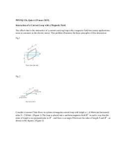
Earth and Planetary Science Letters 420 (2015) 55–65
Contents lists available at ScienceDirect
Earth and Planetary Science Letters
www.elsevier.com/locate/epsl
Resolving the era of river-forming climates on Mars using stratigraphic
logs of river-deposit dimensions
Edwin S. Kite a,b,c,∗,1 , Alan D. Howard d , Antoine Lucas e , Kevin W. Lewis f
a
Princeton University, Department of Geosciences, Princeton, NJ 08544, United States
Princeton University, Department of Astrophysical Sciences, Princeton, NJ 08544, United States
c
University of Chicago, Department of Geophysical Sciences, Hinds Building, 5734 S. Ellis Ave., Chicago, IL 60637, United States
d
University of Virginia, Department of Environmental Sciences, Charlottesville, VA 22904, United States
e
AIM CEA-Saclay, University Paris-Diderot, France
f
Johns Hopkins University, Department of Earth and Planetary Sciences, Baltimore, MD 21218, United States
b
a r t i c l e
i n f o
Article history:
Received 21 October 2014
Received in revised form 3 March 2015
Accepted 6 March 2015
Available online xxxx
Editor: C. Sotin
Keywords:
Mars
paleoclimate
astrobiology
stratigraphy
rivers
a b s t r a c t
River deposits are one of the main lines of evidence that tell us that Mars once had a climate different
from today, and so changes in river deposits with time tell us something about how Mars climate changed
with time. In this study, we focus in on one sedimentary basin – Aeolis Dorsa – which contains an
exceptionally high number of exceptionally well-preserved river deposits that appear to have formed
over an interval of >0.5 Myr. We use changes in the river deposits’ scale with stratigraphic elevation
as a proxy for changes in river paleodischarge. Meander wavelengths tighten upwards and channel
widths narrow upwards, and there is some evidence for a return to wide large-wavelength channels
higher in the stratigraphy. Meander wavelength and channel width covary with stratigraphic elevation.
The factor of 1.5–2 variations in paleochannel dimensions with stratigraphic elevation correspond to
∼2.6-fold variability in bank-forming discharge (using standard wavelength-discharge scalings and widthdischarge scalings). Taken together with evidence from a marker bed for discharge variability at ∼10 m
stratigraphic distances, the variation in the scale of river deposits indicates that bank-forming discharge
varied at both 10 m stratigraphic (102 –106 yr) and ∼100 m stratigraphic (103 –109 yr) scales. Because
these variations are correlated across the basin, they record a change in basin-scale forcing, rather than
smaller-scale internal feedbacks. Changing sediment input leading to a change in characteristic slopes
and/or drainage area could be responsible, and another possibility is changing climate (±50 W/m2 in
peak energy available for snow/ice melt).
© 2015 Elsevier B.V. All rights reserved.
1. Introduction
Many of the now-dry rivers on Mars were once fed by rain or
by snow/ice melt, but physical models for producing that runoff
vary widely (Malin et al., 2010; Mangold et al., 2004; Irwin et
al., 2005a). Possible environmental scenarios range from intermittent <102 yr-duration volcanic- or impact-triggered transients
to >106 yr duration humid greenhouse climates (Andrews-Hanna
and Lewis, 2011; Kite et al., 2013a, 2014; Mischna et al., 2013;
Segura et al., 2013; Urata and Toon, 2013; Tian et al., 2010;
*
Corresponding author at: University of Chicago, Department of Geophysical Sciences, Hinds Building, 5734 S. Ellis Ave., Chicago, IL 60637, United States.
E-mail address: [email protected] (E.S. Kite).
1
Tel.: +1 510 717 520; fax: +1 773 702 0207.
http://dx.doi.org/10.1016/j.epsl.2015.03.019
0012-821X/© 2015 Elsevier B.V. All rights reserved.
Halevy and Head, 2014; Wordsworth et al., 2013; Ramirez et
al., 2014). These diverse possibilities have very different implications for the duration, spatial patchiness, and intermittency of the
wettest (and presumably most habitable) past climates on Mars. As
a set, these models represent an embarrassment of riches for the
Mars research community, and paleo-environmental proxies (ideally, time series) are sorely needed to discriminate between the
models. In principle, discriminating between the models using the
ﬂuvial record should be possible, because runoff intensity, duration and especially intermittency control sediment transport (e.g.
Devauchelle et al., 2012; Morgan et al., 2014; Williams and Weitz,
2014; Erkeling et al., 2012; Kereszturi, 2014; Kleinhans et al., 2010;
Kleinhans, 2005; Lamb et al., 2008; Hauber et al., 2009; Jaumann
et al., 2005; Williams et al., 2011; Leeder et al., 1998; Barnhart et
al., 2009; Howard, 2007). For example, Barnhart et al. (2009) and
Hoke et al. (2011) both use geomorphic evidence for prolonged
56
E.S. Kite et al. / Earth and Planetary Science Letters 420 (2015) 55–65
Fig. 1. Graphical abstract of this study. We measure the width (w) and wavelength (λ) of Mars river-deposits eroding out of the rock, assign stratigraphic elevations zs to
each measurement, and convert these to estimates of paleo-discharge Q ( zs ). Depth of chute cutoff (in left panel) is 2 m.
sediment transport to argue forcefully that impact-generated hypotheses for Early Mars runoff cannot be sustained.
However, geomorphology usually provides time-integrated runoff constraints, whereas constraining climate change requires timeresolved constraints; few locations on Mars show evidence for
more than one river-forming episode; and correlation between
those locations has to rely on crater counting, which (for this application) suffers from small-number statistics, cryptic resurfacing,
target strength effects, confusion between primary and secondary
craters, and inter-analyst variability (e.g. Dundas et al., 2010;
Smith et al., 2008; Warner et al., 2014; Robbins et al., 2014). These
problems have limited the application of dry-river evidence to constrain climate change during the era of river-forming climates on
Mars.
Aeolis Dorsa (1◦ S–8◦ S, 149◦ E–156◦ E) – a wind-exhumed sedimentary basin 10◦ E of Gale crater that contains an exceptionally high number of exceptionally well-preserved river deposits
– gets around these problems. At Aeolis Dorsa, basin-scale mapping distinguishes 102 m-thick river-deposit-hosting units, which
collectively provide time-resolved climate constraints (river valleys provide time-integrated constraints) (Kite et al., 2015). We
can put these deposits in time order using crosscutting relationships, which lack the ambiguity of crater counts. Paleodischarge
can be estimated from meander wavelengths and channel widths
(Burr et al., 2010). Therefore, Aeolis Dorsa contains a stratigraphic
record of climate-driven surface runoff on Mars (Burr et al., 2010;
Fairén et al., 2013; Kite et al., 2015).
To constrain paleodischarge versus time, in this study we measure how river-deposit dimensions vary with stratigraphic elevation (Hajek and Wolinsky, 2012). The key results are set out in
Table 1. We review terrestrial background and geologic context in
Section 1.1. We introduce our method (Fig. 1) in Section 2; this
method is generally applicable to stratigraphic logging from stereopairs (not just logs of river-deposit dimensions). We report our
dataset, describe our paleodischarge interpretation, and discuss the
implications for ﬂuvial intermittency and abrupt climate change
in Section 3. We discuss implications for paleodischarge variability
in Section 4, assess the science merit of landing at Aeolis Dorsa in
Section 5, and conclude in Section 6.
1.1. Fluvial signatures of climate events on Mars: clearer than Earth
Fluvial sediments record climate events in Earth history through
changes in river-deposit dimensions, channel-deposit proportions,
and ﬂuvial styles (e.g. Foreman et al., 2012; Macklin et al., 2012;
Amundson et al., 2012; Schmitz and Pujalte, 2007).
Dry rivers are most useful in reconstructing climate change
when the record is preserved as deposits (as at Aeolis Dorsa) and
when it is uncontaminated by large-amplitude externally-driven
tectonic uplift (as at Aeolis Dorsa). Mars lacks plate tectonics and
Fig. 2. a) Locator map for our study area (red rectangle). Background is shaded relief Mars Orbiter Laser Altimeter (MOLA) topography, illuminated from top right.
Colored contours show output from a seasonal melting model (Kite et al., 2013a:
relative frequency of years with seasonal surface liquid water, average of 88 different orbitally-integrated thin-atmosphere simulations). The black line marks the
border of the area of recently-resurfaced terrain, and approximately corresponds
to the hemispheric dichotomy. This ﬁgure is modiﬁed from Fig. 16d in Kite et al.
(2013a). b) Zooming in to our study area, showing locations of transects (black
rectangles; detail shown in Supplementary Materials Section A2). Transect 1 consists of two nearby non-contiguous areas. Green line shows trace of R-1/R-2 contact
(z s = 0 m). R-2 is above the contact (orange/red tints), and R-1 is below the contact (purple/blue tints). Grey contours are MOLA topography, at 200 m intervals.
Background colors correspond to the elevation from MOLA (blue is low and red
is high). Cyan outlines correspond to large meander belts, which disappear beneath
and reappear from underneath smooth dome-shaped outcrops of R-2. Purple dashed
line outlines an old crater. (For interpretation of the references to color in this ﬁgure legend, the reader is referred to the web version of this article.)
has been tectonically quiescent for >3 Ga (Golombek and Phillips,
2012), making the ﬂuvial record of climate change clearer than
on Earth where the strong effects of base-level ﬂuctuations and
synﬂuvial tectonics complicate interpretation of the ﬂuvial record
in terms of climate change (e.g. Blum and Törnqvist, 2000). Reviewing Earth work, Whittaker (2012) states “If topography forms
a non-unique or diﬃcult-to-decode record of past climate [. . .], it
is likely that the sedimentary record, if and where complete, forms
the best archive of landscape response to past climate.”
The sedimentary record in Aeolis Dorsa is >3 km thick (Kite
et al., 2015), and this study focuses on ∼300 m of stratigraphy
bracketing the contact (green line in Fig. 2b) between two riverdeposit-containing units that show dramatically different erosional
E.S. Kite et al. / Earth and Planetary Science Letters 420 (2015) 55–65
57
expression. These units are termed R-1 (low-standing) and R-2
(high-standing). In both units, river deposits outcrop in plan view.
Preservation quality is better than for any on-land plan-view outcrop on Earth (Fig. 1), and resembles high-resolution 3D seismic
data (e.g. Reijenstein et al., 2011; Hubbard et al., 2011). Cratercounts and stratigraphic analyses (Zimbelman and Scheidt, 2012)
correlate the older rivers that are currently exposed in outcrop to
either the central Hesperian or to the Noachian–Hesperian transition (thought to have been a habitability optimum; e.g., Irwin et
al., 2005b).
2. Getting from stereopairs to stratigraphic logs
We seek constraints on river discharge Q as a function of stratigraphic elevation z s from deposits containing proxy data (such
as channel width w and meander wavelength λ) as a function
of 3D spatial position (latitude, longitude, and elevation). Therefore, we must (1) convert 3D spatial position to z s , and (2)
use a transfer function to convert proxy-data averages to Q ( z s )
(Hajek and Wolinsky, 2012; Irwin et al., 2015; Burr et al., 2010;
Williams et al., 2009). (The following is a brief discussion; for more
details, see the Supplementary Materials.)
The stratigraphic interval of interest is exposed over an area
( A b ) of ∼2 × 104 km2 . Assuming a drainage density of 1/km
(mapped channels), a stratigraphic separation between channels of
10 m, and an averaged preserved thickness of 300 m, the length
of preserved channel deposits in A b is comparable to that of all
channels previously mapped on Mars (∼8 × 105 km; Hynek et al.,
2010). In terrestrial ﬁeldwork we would tackle such data overload by deﬁning transects and measuring a stratigraphic section
along each transect. The analogous procedure to deﬁning a transect for Mars orbiter data is to select high-resolution stereopairs
(each stereopair covers an area of ∼100 km2 A b ), each chosen
to span a wide stratigraphic range. Each stereopair is converted to
a digital terrain model (DTM) and accompanying orthorectiﬁed images using BAE Systems SOCET SET software (Kite et al., 2014). We
use 5 stereo DTMs in total, deﬁning three transects that collectively span the area where R-2 is exposed (Fig. 1; Supplementary
Table 1; Figs. S1–S6). Three of the DTMs come from an area of exceptionally good preservation and dense High-Resolution Imaging
Science Experiment (HiRISE) coverage near 153.6◦ E–6◦ S, which we
term Transect 1.
For each transect, we map out z s by subtracting an interpolated R-1/R-2 contact surface from the topography, so that the
R-1/R-2 contact has z s = 0 m. First we deﬁne the contact surface
between R-1 and R-2 by ﬁtting a surface to points where the large
meander-belts characteristic of R-1 were drowned or blanketed by
smoothly-eroding R-2 deposits. (There is evidence for erosion between R-1 and R-2, so the contact is probably time-transgressive in
detail; Supplementary Materials.) Second-order polynomial ﬁtting
is used; similar results were obtained using other deterministic interpolation methods. The layers are nearly ﬂat (typically <1◦ ), so
the elevation difference is also the stratigraphic offset.
Next, we pick channel centerlines, channel banks, areas of channel deposits, and areas of evidence for lateral migration of channels during aggradation. Every vertex from these picks is tagged
with a stratigraphic elevation z s .
To get λ, each channel centerline is picked 3 times by hand.
We then convert into coordinates of along-centerline distance s
and direction θ and identify half-meanders using inﬂection points
(zero-crossings of ∂θ/∂ s) (Fig. 3) (Howard and Hemberger, 1991).
Sinuosity is deﬁned as along-centerline distance between inﬂection
points divided by straight-line distance between inﬂection points.
Half-meanders with sinuosity <1.1 are rejected. For half-meanders
with sinuosity ≥1.1, we take λ as twice the distance between inﬂection points.
Fig. 3. Wavelength (λ) extraction from repeated ArcGIS traces. Points are uniformly
interpolated along three independent centerline traces (colored dots). Dot color corresponds to the modern topographic range – standard deviation of 4 m in this case.
Lines link inﬂection points (asterisks) that are obtained from each centerline trace.
The low-sinuosity half-meander (arrowed) is excluded from the analysis. (For interpretation of the references to color in this ﬁgure legend, the reader is referred to
the web version of this article.)
To get w, we interpolate equally-spaced points along each bank,
and then ﬁnd the closest distance from each point to the opposing
bank. w is then deﬁned as the median bank-to-bank distance.
We need error bars to avoid overﬁtting models to data. There
are four principal contributors to error: z s error, measurement error, preservation bias, and sampling error. z s error is quantiﬁed
using the root-mean-square error on the interpolated contact surface. The stratigraphic RMS error is 20 m for Transect 1; 5 m for
Transect 2; and 67 m for Transect 3 (Supplementary Methods).
Measurement error is quantiﬁed (for λ) using the variance of λ
extracted from repeated, independent traces on the same channel
centerlines (Fig. 3) and (for w) by using the variance of bankto-bank widths measured at different locations along the channel
trace. Preservation bias refers to erosional narrowing (or widening) of w (Williams et al., 2009). In practice, we found preservation bias to be minor (Section 3.2–Section 3.3, Fig. S7). Sampling
error is quantiﬁed by bootstrapping. Bootstrapping accounts for
the fact that we can only measure the subset of river deposits
that outcrop in our DTM areas, which is a chance sampling from
river-deposits that are dispersed within a three-dimensional rock
volume. When applying the bootstrap, we must combine nonindependent measurements, otherwise the error bars from the
bootstrap will be too small. We therefore treat data points collected from the same channel thread as a single combined measurement. The bootstrap error bars shown in Fig. 4 and Fig. S2
take into account z s error and measurement error as well as sampling errors. We log-transform all data before calculating errors
and averages, because we are interested in relative changes in scale
parameters.
3. Paleohydrology
3.1. River-deposit scale varies systematically upsection
Wavelength λ tightens upwards across the contact (z s = 0 m
in Fig. 4a). In the best-exposed interval (−100 m < z s < 130 m),
small meanders are rare/absent below 0 m, and common above
0 m. Visual inspection of the data suggests that the most natural break in the data (i.e. the paleohydrologically-inferred contact)
is 20 m below the geologically inferred contact (the two-sample
Kolmogorov–Smirnov test statistic is minimized for a breakpoint
at z s = −16.5 m for λ). From 105 Monte Carlo bootstrap trials, in
58
E.S. Kite et al. / Earth and Planetary Science Letters 420 (2015) 55–65
Fig. 4. Width (w) and wavelength (λ) results. The black symbols show the measurements; crosses × for Transect 1, circles ◦ for Transect 2, and diamonds for
Transect 3. The error bars in w and λ differ for each measurement and are shown
individually. The error bars in zs shown in the top left of each plot correspond to
the median z s errors. The red error bars show the mean and standard deviation of
the data in 40 m-wide z s bins (40 m is approximately ∼2× the median zs error).
The blue line shows a running estimate of the average (for a 40 m zs window),
from a bootstrap. The gray lines correspond to the 2-σ errors on the running average from the same bootstrap, which are equivalent to the (2.1%–97.9%) bounds from
the bootstrap. Gaps in the gray and blue lines show range of zs with few or no data.
Fig. S2 shows the z s = −100 m to z s = +100 m interval in more detail. (For interpretation of the references to color in this ﬁgure legend, the reader is referred to
the web version of this article.)
˜ (zs > −20 m) exceed λ˜ (zs < −20 m) (where λ˜ is the
no cases did λ
sample median). The same result was obtained for a break-point at
z s = 0 m. The trends are consistent between Transect 1 and Transect 2 (Figs. S3, S5–S6).
w also narrows upwards across the contact (z s = 0 m in
Fig. 4b). In the best-exposed interval (−100 m < z s < 130 m), nar-
row channels are rare/absent below 0 m, and common above 0 m.
Similar to λ, visual inspection of the data suggests that the most
natural break in the data (i.e. the paleohydrologically-inferred contact) is z s ∼ −20 m below the geologically inferred contact. (The
two-sample K–S test statistic is minimized for a breakpoint at
z s = +16 m, which reﬂects the greater density of data points at
z s = +20 m to +50 m.) From 105 Monte Carlo bootstrap trials,
in only 1 case the median w above −20 m exceeded the median w below −20 m. For a break-point at z s = 0 m, the same
˜ (zs < −20 m) <
test showed that only 9 cases out of 105 with w
˜ (zs > −20 m). The trends are consistent between Transect 1 and
w
Transect 2 (Figs. S5–S6).
Width w and wavelength λ are poorly constrained for z s >
130 m. There is some evidence for a return to bigger rivers at
higher z s . While there are relatively few data points here (all from
Transect 3; diamonds), the trend to higher λ and w in Transect 3
is statistically signiﬁcant and visually obvious in the DTMs. However, assigning Transect 3 data points to z s > 130 m is only correct
if we assume that the topographic offset between the large rivers
in Transect 3 and the large rivers in Transect 1 (Fig. 2b) corresponds to a stratigraphic offset. This assumption could be wrong
if the river-deposits measured in Transect 3 are separated from
the river-deposits measured in Transects 1 and 2 by a drainage
divide (Kite et al., 2015). Drainage divides can separate nearby
rivers formed at the same time and with large topographic offsets (e.g., Eastern Continental Drainage Divide, Blue Ridge Scarp,
North Carolina, USA). The topographically-offset Transect 3 deposits could be stratigraphically equivalent to the big river-deposits
at z s ≈ −50 m in Fig. 4 if they are separated from them by a
drainage divide. The drainage divide possibility could be tested in
future by using meander-migration directions to test for paleoﬂow
direction.
Sinuosity decreases upsection (Fig. S4) but stays low for Transect 3.
Cross-checking of widths and wavelengths suggests that our
measurements of w have comparable reliability to our measurements of λ (Fig. 5a). This is surprising, because it is much easier
for erosion to narrow inverted channels (Williams et al., 2009) and
widen valleys than to signiﬁcantly modify λ. This consistency reﬂects good preservation of ﬂuvial form.2
To support our scale measurements, we record the channeldeposit outcrop proportion and the fractional exposure of lateral
accretion deposits versus z s (Fig. 5b). Channel-deposit proportion
is high where river-deposit dimensions are large. Evidence for lateral migration of channels during aggradation is frequent where
rivers are large, and very uncommon where rivers are small. Results are very similar in both Transect 1 and Transect 2 (not
shown).
All these metrics are self-consistent, as expected: larger width
rivers should make proportionally larger meander bends (with
w : λ ≈ 10, as observed), and should also migrate laterally at faster
rates.
2
In spite of our expectation that preserved w would be a poor paleodischarge
˜ : λ˜ is consistent with measurements of Earth rivers (Bridge,
proxy, we ﬁnd that: w
2003); inverted-channel w is not signiﬁcantly narrower than negative-relief w
(Fig. S6); the fractional standard deviations of w for a given zs are comparable to
those for λ (Fig. 4); for those λ for which w was also measured, most have a w : λ
ratio within range of terrestrial measurements (Fig. S7); and, again for {λ, w } pairs,
there is no evidence for w : λ ratio changing with zs . With hindsight, this consistency is likely aided by intentional selection of only the best-preserved stretches of
channel in each DTM. From that subset of measured channels, those that showed
signs of relatively more severe erosion were rejected as “candidates.” This left a
fairly restricted set of relatively high-quality measurements. An unrestricted sampling of all channel stretches without consideration of preservation quality would
provide less reliable width measurements.
E.S. Kite et al. / Earth and Planetary Science Letters 420 (2015) 55–65
59
Table 1
Paleodischarge Q versus stratigraphic elevation zs from transects in S. Aeolis Dorsa.
λ˜
(m)
˜
Bankfull Q from λ
(m3 s−1 )
˜
w
(m)
˜
Bankfull Q from w
(m3 s−1 )
Interpolated z s
100 m > z s > −20 m
z s < −20 m
(246 ± 15) m
(466 ± 35) m
(37 ± 3) m3 s−1
(99 ± 12) m3 s−1
(25 ± 1.5) m
(43 ± 3.7) m
(28 ± 3) m3 s−1
(76 ± 12) m3 s−1
Interpolated z s
100 m > z s > 0 m
zs < 0 m
(229 ± 14) m
(432 ± 31) m
(33 ± 3) m3 s−1
(89 ± 10) m3 s−1
(25 ± 1.5) m
(37 ± 3.2) m
(28 ± 3) m3 s−1
(58 ± 9) m3 s−1
(31 ± 3) m3 s−1
(80 ± 9) m3 s−1
(213 ± 35) m3 s−1
(22 ± 1.5) m
(37 ± 3.0) m
(61 ± 13) m
(22 ± 3) m3 s−1
(58 ± 9) m3 s−1
(147 ± 58) m3 s−1
Unit assigned from mapping (no interpolation)
R-2
(219 ± 14) m
R-1
(406 ± 29) m
Transect 3
(764 ± 82) m
3.2. Evidence for basin-wide paleo-discharge variability
˜ and w
˜ that is apparent in both TranThe decrease in both λ
sect 1 and Transect 2 (Fig. 4) is representative of a basin-wide
˜ and w
˜
change in channel-deposit dimensions. The reduction in λ
upsection is visually obvious in the transect DTMs (Fig. S1) and
also in ConTeXt Camera (CTX) mosaics spanning the full area of
the R-1/R-2 contact. Basinwide, R-1 erodes to form yardangs and
is very rough at km scales, not retaining recognizable craters; river
deposits in R-1 formed large meanders and broad meander belts.
Basinwide, R-2 is topographically high-standing, smoothly eroding, associated with numerous aeolian bedforms, and retains many
craters. River deposits in R-2 left narrow channel deposits and
formed tight meanders. The basin-wide spatial scale and ∼100 m
stratigraphic scale of the changes we report in this study probably
puts them beyond the grasp of shredding of environmental signals by nonlinear sediment transport (Jerolmack and Paola, 2010;
Sadler and Jerolmack, 2014).
Motivated by the coherence of our paleohydrologic proxies –
between metrics and between transects (Figs. S3–S6) – we conclude that R-2 records a distinct episode of runoff from R-1. We
now turn to quantifying the change in discharge across the contact
by using λ and w as proxies for Q .
For rivers on Earth, bank-full discharge Q scales approximately
as w 2 and as λ2 . The physical basis for this increase (Finnegan
et al., 2005) is that channel depth h tends to increase in proportion with w, whereas water velocity u increases only sluggishly
with w. Since Q = whu (by continuity), Q ∝ w ∼2 . Theory suggests that initially-straight rivers are most vulnerable to sinuous
instabilities with λ ∼ 10w (bar-bend theory) (Blondeaux and Seminara, 1985), and that as the meander amplitude grows, the wavelength of the initial instability is frozen-in to the growing meander
(Bridge, 2003). Therefore λ ∝ w (Bridge, 2003).
We adopt the Eaton (2013) scaling for w and the Burr et al.
(2010) scaling for λ. Rivers on Mars are expected to ﬂow slower
than rivers on Earth because Martian gravity is lower. Theoretically, w ∝ g −0.2335 (Parker et al., 2007), so we divide the widths
by (Mars gravity/Earth gravity)−0.2335 = 1.257. Therefore:
1.8656
Q = w /(1.257 × 3.35)
(1)
Q = 0.011(λ/1.267)1.54
(2)
3,4
We report ‘nominal’ bank-full discharges in Table 1.
Fig. 5. Summary of results, combining all transects. a) Comparison of width (w) and
wavelength (λ) results. Error bars show 1σ spread of measurements (averaged in
40 m z s bins). Numbers next to error bars correspond to the number of measurements. b) Areal fractions of channel deposits (thick line) and of deposits showing
evidence for lateral accretion (thin line). zs bin size = 10 m.
3
More sophisticated approaches to estimating paleo-discharge require slope
and/or grain-size information. Unfortunately, in southern Aeolis Dorsa, the presentday slopes of the river deposits are unlikely to be a safe guide to the slopes when
the rivers were ﬂowing (Lefort et al., 2012), and clasts are not seen in HiRISE images.
4
w–Q relationships in ice-ﬂoored channels are poorly constrained (e.g.
McNamara and Kane, 2009). Strong banks are needed for meandering; on Mars,
60
E.S. Kite et al. / Earth and Planetary Science Letters 420 (2015) 55–65
wind-blown: in Aeolis Dorsa, areas that were once wet (e.g.,
meander belts, channels) are preferentially preserved against
modern wind erosion.
Fig. 6. Evidence for intermittency at approximately 10 m stratigraphic scale from
DTM constructed from PSP_006683_1740 and PSP_010322_1740. Image is 4.2 km
across. The less-sinuous inverted channel is ∼10 m above the more-sinuous early
meander belt. The full range of topography in the DTM is ∼30 m (which may include postdepositional tilting; Lefort et al., 2012). Earlier channel generations which
were crosscut by the early meander belt are visible in top right (pooly-preserved
sinuous ridges).
Paleo-discharges inferred for unit R-1 are higher than those for
R-2 by ∼260%. This does not depend on how the breakpoint is
deﬁned (Table 1). Q λ is higher than Q w , but within the standard
error of the terrestrial regressions (41% standard error for λ, and
29% for w) (Burr et al., 2010; Eaton, 2013). This difference might
be caused by erosional narrowing of channel widths.
In addition to the large-scale changes shown in Table 1, our
DTMs record paleodischarge variability at z s scales too ﬁne to be
resolved in our stratigraphic logs. For example, Fig. 6 shows a lowsinuosity inverted channel without cutoffs that follows the trend
of a very sinuous meander-belt deposit with numerous cutoffs
(Burr et al., 2010; Jacobsen and Burr, 2013; Cardenas and Mohrig,
2014). The inverted channel is ∼10 m above the meander belt.
This sequence is widespread in southeast Aeolis Dorsa (e.g. HiRISE
images ESP_036378_1740 and PSP_008621_1750). We interpret
this pattern as a stratigraphic marker of a basinwide event (rather
than the result of uncorrelated avulsions), because the pattern is
never seen at more than 1 stratigraphic level locally, has a common erosional expression basinwide, joins at conﬂuences, and is
only found just below the R-1/R-2 contact. The following cut-andﬁll sequence may explain these observations:
• Rivers transported sediment for long enough to develop highsinuosity channels and a broad meander belt with cutoffs.
• Fluvial sediment transport ceased, or was diverted. The
meander-belts were then covered by ∼10 m of now-removed
cover material, which inﬁlled the channels but failed to completely mute the paleo-valleys containing the meander-belts.
• The channel-belt cover was re-incised by rivers that followed
the trend of the partly-inﬁlled valleys.
• Fluvial sediment transport shut down again – after a shorter
period of ﬂuvial activity than for the ﬁrst-generation channels
– and the less-sinuous valley was itself inﬁlled.
• Late-stage erosion removed the cover material, causing pronounced topographic inversion of the less-sinuous channel
and partial topographic inversion of the more-sinuous channel. Preferential removal of the cover material by wind erosion is consistent with the idea that the cover material was
ice, salt or clay could ﬁrm up banks (Matsubara and Howard, 2014; Matsubara et
al., 2015).
The inferred switching from ﬂuvial sediment transport, to inﬁlling/mantling, followed by ﬂuvial re-incision, is consistent with
a wet–dry–wet sequence (Metz et al., 2009; Williams and Weitz,
2014). We also ﬁnd cut-and-ﬁll cycles in R-2, with stratigraphic
amplitude ∼3 m. However, there is no requirement from our DTMs
that peak ﬂows during the event that formed the less-sinuous
channels were less than peak ﬂows during the event that formed
the more-sinuous underlying meander belt. We hand-tagged λ and
w measurements in our DTMs corresponding to the two layers
(which are visually distinctive and easy to identify; Fig. 6). We
ﬁnd λ = 588(+631/−304) m (n = 8) for the more-sinuous meander belt and λ = 421(+191/−132) m (n = 13) for the less-sinuous
inverted channel. These results overlap, although the more-sinuous
meander belt does have some tight, short-wavelength meanders
which are not found in the less-sinuous inverted channel. We ﬁnd
w = 46(+18/−13) m (n = 19) in the more sinuous meander belt
and w = 39(+12/−9) m (n = 11) for the less sinuous member.
These results are not signiﬁcantly different.
3.3. Both short-term intermittency and long-term intermittency are
required
There is evidence for intermittency at four different stratigraphic scales in Aeolis Dorsa. (1) Erosion-deposition alternations
suggest wet–dry alternations in Aeolis Dorsa at the stratigraphic
scale of hundreds of meters to kilometers (Kite et al., 2015). Aeolis Dorsa’s >3 km of stratigraphy consists of four rock packages
bounded by unconformities. The top three rock packages probably required near-surface liquid water to make rivers, make alluvial fans, and cement layers. The unconformities show erosion
and interbedded craters suggesting long time gaps (Kite et al.,
2015). Aeolian erosion during these time gaps is suggested by
smooth deﬂation at the unconformities, and if surface liquid water
been available it would have suppressed aeolian erosion by trapping the clasts needed for wind-induced saltation abrasion. (2) At
100 m stratigraphic scale, our logging suggests variations in discharge (Figs. 4–5). (3) At 10 m stratigraphic scale, we interpret
the stratigraphy of the marker bed (Fig. 6) to suggest wet–dry–wet
alternations. (4) At 1 m stratigraphic scale, chute cutoffs indicate
discharge variability, and it is also tempting to interpret the 2–3 m
banding in the lateral-accretion deposits as the result of annual
ﬂoods.
What was the timescale for these processes? The high density of embedded impact craters suggests a depositional interval of
>(4–20) Myr (Kite et al., 2013b). This method does not constrain
whether deposition was steady or pulsed. Sediment transport calculations provide an estimate of the intermittency. To re-incise a
fresh channel such as the low-sinuosity inverted channel in Fig. 6,
the volume of the channel must be transported downstream as
sediment (Church, 2006). Therefore τ = L c wh/( Q f sed ), where τ is
timescale, L c is channel length, h is channel depth, Q is water
discharge, and f sed 1 is sediment fraction. Setting L c ≈ 102 km
(Fig. 2b), w ≈ 40 m (Table 1), h ≈ w /57 (Hajek and Wolinsky,
2012; Gibling, 2006), Q ≈ 80 m3 /s, and f sed = 1–2 × 10−4 (Palucis
et al., 2014), we obtain τ ≈ 0.15–0.3 yr. If the entire volume of
unit R-1 was transported by rivers, τ = z s A b /( N r Q f sed ) where
zs is unit thickness and N r is the number of rivers. Assuming
rivers at indistinguishable stratigraphic levels were active simultaneously, N r ≈ 20. With z s ≈ 300 m (Kite et al., 2015), we obtain τ = 0.5–1 Myr. At long-term terrestrial ﬂoodplain aggradation
rates z s ≈ 300 m corresponds to a time interval of 1.5 × 104 –9 ×
105 yr (Bridge and Leeder, 1979). These values are all less than the
E.S. Kite et al. / Earth and Planetary Science Letters 420 (2015) 55–65
61
Fig. 7. a) Abrupt climate change detection concept. b) Idealized outcomes. c) Application to synthetic dataset with real errors and stratigraphic elevations, and artiﬁcially-sharp
breakpoints in λ and w. d) Application to Aeolis Dorsa observations.
estimate from embedded-crater density, consistent with intermittency, although the error bars are large (e.g., Buhler et al., 2014;
Irwin et al., 2015).
It would be interesting to incorporate ﬂuvial intermittency as
a constraint on numerical simulations of catchment response to
climate change (Armitage et al., 2013) and to investigate whether
lower limits on the duration of Mars river activity can be inferred
from the spatial scales at which cut-and-ﬁll cycles are correlated
across catchments and across the basin.
3.4. A tool to search for abrupt climate change on Mars
To search for paleohydrologic evidence of stratigraphically
abrupt climate change on Mars, we analyze our dataset to see
if it contains a sharp transition in river-deposit dimensions that
is robust against the errors captured by our bootstrap procedure.
To do this, we use the K–S test to ﬁnd breakpoints for each of an
ensemble of bootstrapped datasets. For each bootstrapped dataset,
we deﬁne z∗s as the z s that minimizes the K–S statistic (i.e., the z s
corresponding to the most statistically-signiﬁcant breakpoint between data above z s and data below z s ). We ﬁnd z∗s for every
bootstrapped distribution of data in the ensemble. If abrupt climate
change had occurred, then z∗s would vary little between the members of the ensemble – it would be tightly clustered in z s (Fig. 7b).
If instead climate change was only gradual, then we would expect
to see a broad distribution of z∗s (Fig. 7b).
Wide error bars can produce false negatives for abrupt climate
change. To demonstrate that our dataset is rich enough to detect an abrupt climate change (had it occurred), we generate a
synthetic dataset that has the same error bars and z s values as
the observations, but has λ and w set to a uniform value below
z s = 0 m and set to a different uniform value above z s = 0 m. We
recover a sharp break in both λ and w at z s ≈ 0 m after passing the synthetic dataset through our algorithm (Fig. 7c), which
shows that for this dataset our abrupt-change detection scheme is
unbiased and robust to false negatives. Finally, we use the observations (Fig. 7d). (Transect 3 data points were excluded.) We ﬁnd
that z∗s is fairly widely scattered in both λ and w (5%–95% range
of z∗s is 35 m for λ and 90 m for w). We conclude that our stratigraphic logs do not require stratigraphically abrupt climate change
on Mars.
4. Implications for river-forming paleo-climates on Mars
4.1. Mechanisms for paleodischarge variability
Our preferred explanation for the { w, λ} changes is a decrease in runoff production (i.e., climate change) (Foreman et al.,
2012). The required relative change in runoff production for constant drainage area A d is a factor of ∼2.6 (Table 1) ( A d = L /dd ,
where L is the distance to the drainage divides and dd is drainage
density). An estimate of A d allows constraints on absolute changes
in runoff production. For R-1, a lower bound on L is the distance to
the tips of the presently-preserved channel network (∼40 km); an
upper bound is the distance to the dichotomy scarp (∼200 km to
the S). The R-1 drainage density is assumed constant at 0.2 km−1 .
For R-2, a lower bound on L is the length of currently-exposed
channels (∼10 km). The upper limit is again the distance to the
dichotomy scarp. The R-2 drainage density is assumed constant
at 1 km−1 . More precise estimates are diﬃcult because erosion
has removed the drainage divides of the catchments feeding the
rivers preserved in our transects. Near-surface hydraulic conductivity is assumed not to change with time (not unreasonable in
an aggrading system). We express the required change in runoff
production (Fig. 8) in terms of the energy available for melting
snow/ice E melt = Q ρ c / A, where c is the latent heat of melting ice
(334 kJ/kg) and ρ is the density of water. (None of the data presented in this study argues against rainfall providing the runoff
for the Aeolis Dorsa rivers; using E melt is simply a convenient way
of expressing the energy budget). The preferred drainage area is
∼400 km2 , for which peak melt energy (peak runoff production)
decreases from 63–83 W/m2 (dividing this value by the latent
heat of melting ice and the density of water gives 0.7–0.9 mm/hr)
for R-1, to 23–31 W/m2 (∼0.3 mm/hr) for R-2. For the relatively
large catchments studied here, this should probably be interpreted
as a constraint on daily-average runoff production. The absolute
magnitude of change scales inversely with A d , and because A d is
poorly constrained we regard the absolute magnitude with some
suspicion. However, a reduction of 50 W/m2 in E melt could result from a number of non-exotic processes. Examples include a
rise in albedo from 0.2 to 0.3, a decrease in peak eccentricity from
0.14 to 0.1, or a decline in atmospheric pressure from ∼100 mbar
to ∼40 mbar with a corresponding increase in evaporitic cooling
(Kite et al., 2013a; Mischna et al., 2013).
Three-fold Q variability does not exclude quasi-periodic orbital
forcing. Small variations between successive peaks in orbital forcing can lead to large differences in Q . Thresholds amplify input
62
E.S. Kite et al. / Earth and Planetary Science Letters 420 (2015) 55–65
roughens the landscape between R-1 and R-2 time (an Earth example is described in Haberlah et al., 2010) and breaks up the
smooth alluvial R-1 landscape into small catchments, and these
small catchments are not integrated by the R-2 rivers. The R-2
channels have a network pattern that is hard to reconcile with
the aeolian-roughening hypothesis. Drainage along linear interdunes would leave a linear channel pattern, but the R-2 networks
lack this pattern. We also cannot rule out reduction in A d due to
drainage capture by catchments to the south. These A d -change scenarios assume paleo-drainage to the N in R-1/R-2, which is our
preferred interpretation in part because the regional tilt is to the
north. If paleo-drainage was instead directed to the south, then
variation in A d is even less likely because river-long-proﬁle distances in Aeolis Dorsa can exceed >500 km (Williams et al., 2013);
such large catchments would evolve slowly (Armitage et al., 2013).
Fig. 8. The horizontal lines show runoff constraints for R-1 and R-2, and the vertical
dashed lines show estimated drainage areas. The thick red curve shows diurnallyaveraged equatorial perihelion equinox insolation for an eccentricity of 0.12 and
solar luminosity of 80% that of present. The thick brown curve shows noontime
equatorial perihelion equinox insolation for an eccentricity of 0.12, solar luminosity
80% that of present. The discharge curves make the unrealistic assumption that melt
energy is equal to insolation, and so serves as an upper limit on insolation. There is
also the issue of ﬂow routing through the drainage network, tending to reduce ﬂood
peaks, and the necessity for discharge to be routed over distances >10 km. The thin
colored curves are labeled with log10 (melt energy) in units of log10 (W)/m2 . The
black arrows show pathways for climate change (vertical black arrow) and changing
drainage area (oblique black arrow). (For interpretation of the references to color in
this ﬁgure legend, the reader is referred to the web version of this article.)
variations (Huybers and Wunsch, 2003), and there are multiple
thresholds in the chain of processes linking insolation to carving a river. For example, melting initiates at 273 K, overland ﬂow
only occurs when melt exceeds inﬁltration capacity, and sediment
movement begins above a critical Shields stress.
Inferred Q variations are completely inconsistent with monotonically decreasing rainfall following an impact, but more sophisticated models of impact-triggered rainfall show seasonal variations (Segura et al., 2013). If an impact triggered a metastable
greenhouse (e.g. Urata and Toon, 2013; Segura et al., 2013; Toon
et al., 2010) then season and orbital variability would be expected.
A change in w need not imply a change in Q – if slope S
steepens, rivers ﬂow faster, and the same discharge is conveyed
by a narrower channel. Field measurements and theory show that
w ∝ S −3/16 (Lee and Julien, 2006; Finnegan et al., 2005). Therefore, a 100-fold increase in S between R-1 and R-2 could cause
the ∼2 fold reduction in { w , λ}. While recognizing the potential
complication of post-depositional tilting (Lefort et al., 2012, 2015),
the present-day tilt is ∼0.01 to the north for R-2 channels in
our DTMs, so supposing S = 10−4 for R-1 channels, the 100-fold
increase in S between R-2 and R-1 channels can explain w reductions. In order for S to increase within an aggrading sediment
package in the absence of changes in discharge or changes in tectonic boundary conditions, either a coarsening of input grain-size
or an increase in the rate of non-ﬂuvial sediment input is required. (Flexure under the sediment load would most likely lead
to southward tilting, which has the wrong sign to explain the observations.) Although slope increase may have occurred, we do not
believe this is suﬃcient to explain the observed narrowing because
a slope of 0.01 over the 40 km N–S extent of R-2 outcrop implies
a wedge of sediment thickening to 0.4 km. No such wedge is observed; instead, additional units lacking embedded ﬂuvial deposits
are exposed in scarps to the S of the area shown in Fig. 2b (Kite et
al., 2015) and we interpret these units to have formerly extended
out over the area of our transects.
Another scenario in which w is reduced without a change in
Q is if A d is reduced upsection. In this picture, aeolian sediment
4.2. Global context
Our Aeolis Dorsa results add strength to an emerging global picture of time-variable, intermittent, occasionally voluminous river
discharge driven by wet paleoclimates and extending remarkably
late in Mars history (e.g. Weitz et al., 2013; Grant and Wilson,
2011, 2012; Fassett et al., 2010; Williams and Weitz, 2014). Intermittency is required to explain closed crater-lake basins containing deltas and fed by channels with measured widths because continuous ﬂow would overspill the closed basin, incise an
exit channel, and breach the crater rim (Matsubara et al., 2011;
Irwin et al., 2007; Lewis and Aharonson, 2006; Buhler et al., 2014;
Mangold et al., 2012). Fluvial intermittency is also required to account for indurated aeolian bedforms interbedded with river/lake
deposits (Milliken et al., 2014; Williams and Weitz, 2014). Large
alluvial fans prograding into crater ﬂoors lacking deep paleolakes
also set limits on discharge magnitude and duration (e.g., Morgan
et al., 2014). Our 0.5–1 Myr estimated duration of wet conditions
is consistent with estimates elsewhere on Mars (using erosional
timescales, e.g. Hoke et al., 2011, or sedimentary deposits, e.g. Armitage et al., 2011). However, because of erosion and burial, these
estimates could correspond to totally distinct episodes. Mineralogic
constraints complement geomorphic constraints. Mineralogy suggests pervasive, generally isochemical alteration at low water/rock
ratio with preferential dissolution of olivine (e.g. Olsen and Rimstidt, 2007; Hurowitz and McLennan, 2007; Berger et al., 2009;
Carter et al., 2012; Elwood Madden et al., 2009; Bandﬁeld et al.,
2011; Ehlmann et al., 2011; McLennan et al., 2014). In particular, orbiter detections of aqueous minerals associated with wellpreserved ﬂuvial features are limited to opal and detrital clays (e.g.,
Milliken and Bish, 2010).
An open question is whether the probability density function
(pdf) of post-Noachian Mars surface habitability was bimodal or
unimodal. In the unimodal hypothesis, post-Noachian rivers record
orbital-forcing optima of a long-term climate evolution driven by
unidirectional atmospheric loss and increasing solar luminosity
and perturbed by stochastic orbital variability. The unimodal hypothesis is attractively simple, but sets a challenge for the modeling community: can a “wet tail” climate-evolution scenario that
generates peak runoff high enough to account for rivers like those
in Aeolis Dorsa avoid breaching mineralogical upper limits on total liquid water availability (e.g. Tosca and Knoll, 2009)? If not,
then late-stage rivers would require a bimodal climate evolution
pdf – in which post-Noachian rivers record a discrete class of
(metastable?) more-habitable climates.
5. Habitability, taphonomy, and organic matter preservation
The search for life on Mars has narrowed to a search for ancient
biogenic organic matter (Farmer and Des Marais, 1999; Grotzinger,
E.S. Kite et al. / Earth and Planetary Science Letters 420 (2015) 55–65
2014). In order for ancient complex biogenic organic matter to
be present in the near-surface today, the paleo-environment must
have been habitable, with high organic-matter preservation potential; and the rocks must have been rapidly exhumed to minimize radiolysis. In Aeolis Dorsa, meander cutoffs deﬁne oxbow
lakes, which are favored for the preservation of ﬁne-grained sediments that tend to bind organic matter (Constantine et al., 2010;
Ehlmann et al., 2008). River ﬂoodplains have better organic-matter
preservation potential than aeolian deposits, alluvial-fan deposits,
or ﬂuvial-channel deposits, although distal lacustrine sites are better still (Summons et al., 2011; Williams and Weitz, 2014). Aeolis Dorsa river discharges and ﬂow durations suggest a habitable environment, the relatively high deposition rates favor preservation against early degradation, and the relatively high erosion
rate protects against radiolysis during exhumation. In particular,
a 3000 km2 area around Transect 1 lacks craters larger than D >
1 km, corresponding to a nominal erosion rate of 0.2–0.4 μm/yr
(using the chronology of Werner and Tanaka, 2011). This is suﬃciently high to minimize radiolysis of complex organic matter at
the depths sampled by Mars 2020 (several cm) and the ExoMars
rover (≤2 m) (Pavlov et al., 2012; Farley et al., 2014). Therefore the
river deposits we document are a promising alternative for paleobiological exploration in the event that suitable lacustrine deposits
cannot be identiﬁed and sampled in situ.
6. Conclusions
We analyze past river processes at Aeolis Dorsa, Mars, by
collapsing measurements of river-deposit dimensions onto stratigraphic logs.5 Our stratigraphic logs show a (1.5–2)× reduction in
river-deposit dimensions between two river deposits. This is consistent with a 2.6× reduction in peak discharge across the contact,
using size-discharge scalings modiﬁed for Mars gravity. Markerbed stratigraphy suggests additional variations in peak discharge
at stratigraphic scales below the resolution of the logs. The total
time interval for these changes probably exceeded 0.5 Myr. Similar
to the Grand Staircase, Utah, USA, at Aeolis Dorsa we see multiple
layers of ancient river deposits exposed by modern erosion. The
requirement for intermittency at multiple timescales (as shown
by river-deposit dimensions, regional unconformities, and marker
beds) is a stringent constraint on quantitative models linking ﬂuvial sedimentology to late-stage climate evolution.
Acknowledgements
This paper grew from discussions in the Caltech Mars Fluvial Geomorphology Reading Group, and we thank all the participants, especially Mike Lamb and Roman DiBiase. To the extent we understand Aeolis Dorsa, it is thanks to conversations
with the following scientists, who we have relied heavily on
in thinking through this problem: Alexandra LeFort, Laura Kerber, Caleb Fassett, Noah Finnegan, Lynn Carter, Nicolas Mangold,
Sanjeev Gupta, Matt Balme, Sam Harrison, Maarten Kleinhans,
Leif Karlstrom, David Mohrig, Benjamin Cardenas, Jim Zimbelman, Steve Scheidt, Michael Manga, Bill Dietrich, Ross Irwin, Jeff
Moore, Christian Braudrick, Devon Burr, Robert Jacobsen, Noah
Finnegan, Jonathan Stock, Gary Kocurek, Richard Heermance, Paul
E. Olsen, Or Bialik, Brian Hynek. We thank Robert Jacobsen for
comments on a draft. E.S.K. thanks Ross Beyer, Sarah Mattson,
Annie Howington-Kraus, and Cynthia Phillips for help with generating the PSP_006683_1740/PSP_010322_1740 DTM. E.S.K. was
5
This technique may be particularly useful for extracting records from HighResolution Stereo Camera (HRSC)/Mars Express data and from Color and Stereo
Surface Imaging System (CaSSIS)/ExoMars Trace Gas Orbiter data.
63
supported by a Princeton University fellowship and by NASA grant
NNX11AF51G. We thank the HiRISE team for maintaining the
HiWish program, which supplied multiple images essential for this
study.
Appendix A. Supplementary material
Supplementary material related to this article (describing
stratigraphic-elevation assignments, paleohydraulic-proxy measurements and locations, and details on data reduction, as well
as transect-by-transect stratigraphic logs) can be found online at
http://dx.doi.org/10.1016/j.epsl.2015.03.019.
References
Amundson, R., Dietrich, W., Bellugi, D., Ewing, S., Nishiizumi, K., Chong, G., Owen, J.,
Finkel, R., Heimsath, A., Stewart, B., Caffee, M., 2012. Geomorphologic evidence
for the late Pliocene onset of hyperaridity in the Atacama Desert. Geol. Soc. Am.
Bull. 124 (7–8), 1048–1070.
Andrews-Hanna, J.C., Lewis, K.W., 2011. Early Mars hydrology: 2. Hydrological evolution in the Noachian and Hesperian epochs. J. Geophys. Res. 116. CiteID E02007.
Armitage, John J., Warner, Nicholas H., Goddard, Kate, Gupta, Sanjeev, 2011.
Timescales of alluvial fan development by precipitation on Mars. Geophys. Res.
Lett. 38 (17). CiteID L17203.
Armitage, J., Dunkley Jones, T., Duller, R., Whittaker, A., Allen, P., 2013. Temporal
buffering of climate-driven sediment ﬂux cycles by transient catchment response. Earth Planet. Sci. Lett. 369–370, 200–210.
Bandﬁeld, J.L., Rogers, A.D., Edwards, C.S., 2011. The role of aqueous alteration in the
formation of martian soils. Icarus 211, 157–171.
Barnhart, C.J., Howard, A.D., Moore, J.M., 2009. Long-term precipitation and latestage valley network formation: landform simulations of Parana Basin, Mars.
J. Geophys. Res. 114. CiteID E01003.
Berger, G., et al., 2009. Evidence in favor of small amounts of ephemeral and
transient water during alteration at Meridiani Planum, Mars. Am. Mineral. 94,
1279–1282.
Blondeaux, P., Seminara, G., 1985. A uniﬁed bar–bend theory of river meanders.
J. Fluid Mech. 157, 449–470. http://dx.doi.org/10.1017/S0022112085002440.
Blum, M.D., Törnqvist, T.E., 2000. Fluvial responses to climate and sea-level change:
a review and look forward. Sedimentology 47, 2–48. http://dx.doi.org/10.1046/
j.1365-3091.2000.00008.x.
Bridge, J., 2003. Rivers and Floodplains: Forms, Processes, and Sedimentary Record.
Wiley–Blackwell. 504 pp.
Bridge, J.S., Leeder, M.R., 1979. A simulation model of alluvial stratigraphy. Sedimentology 26, 617–644.
Buhler, P.B., Fassett, C.I., Head III, J.W., Lamb, M.P., 2014. Timescales of ﬂuvial activity
and intermittency in Milna Crater, Mars. Icarus 241, 130–147.
Burr, D., et al., 2010. Inverted ﬂuvial features in the Aeolis/Zephyria Plana region,
Mars: formation mechanism and initial paleodischarge estimates. J. Geophys.
Res. 115 (E7). CiteID E07011.
Cardenas, B.T., Mohrig, D., 2014. Evidence for shoreline-controlled changes in baselevel from ﬂuvial deposits at Aeolis Dorsa, Mars. In: 45th Lunar and Planetary
Science Conference. LPI Contribution No. 1777, p. 1632.
Carter, J., et al., 2012. Composition of Deltas and Alluvial Fans on Mars. In: 43rd
Lunar and Planetary Science Conference. March 19–23, 2012, Woodlands, TX.
LPI Contribution No. 1659, id.1978.
Church, M., 2006. Bed material transport and the morphology of alluvial river channels. Annu. Rev. Earth Planet. Sci. 34, 325–354.
Constantine, J.A., et al., 2010. Controls on the alluviation of oxbow lakes by
bed-material load along the Sacramento River, California. Sedimentology 57,
389–407.
Devauchelle, O., Petroff, A.P., Seybold, H.F., Rothman, D.H., 2012. Ramiﬁcation of
stream networks. Proc. Natl. Acad. Sci. 109, 51.
Dundas, C.M., et al., 2010. Role of material properties in the cratering record of
young platy-ridged lava on Mars. Geophys. Res. Lett. 37, L12203.
Eaton, B.C., 2013. Chapter 9.18: Hydraulic geometry. In: Wohl, E.E. (Ed.), Treatise on
Geomorphology, vol. 9, Fluvial Geomorphology. Elsevier, Oxford, UK.
Ehlmann, B.L., et al., 2008. Clay minerals in delta deposits and organic preservation
potential on Mars. Nat. Geosci. 1, 355–358.
Ehlmann, B.L., et al., 2011. Subsurface water and clay mineral formation during the
early history of Mars. Nature 479, 53–60.
Elwood Madden, M., Madden, A., Rimstidt, J., 2009. How long was Meridiani Planum
wet? Applying a jarosite stopwatch to constrain the duration of diagenesis. Geology 37, 635–638.
Erkeling, G., et al., 2012. Valleys, paleolakes and possible shorelines at the Libya
Montes/Isidis boundary: implications for the hydrologic evolution of Mars.
Icarus 219, 393–413.
64
E.S. Kite et al. / Earth and Planetary Science Letters 420 (2015) 55–65
Fairén, A.G., Davies, N.S., Squyres, S.W., 2013. Equatorial ground ice and meandering rivers on Mars. In: 44th Lunar and Planetary Science Conference. Abstract
No. 2948.
Farley, K.A., et al., 2014. In situ radiometric and exposure age dating of the Martian
surface. Science 343 (6169). http://dx.doi.org/10.1126/science.1247166.
Farmer, J.D., Des Marais, D.J., 1999. Exploring for a record of ancient Martian life.
J. Geophys. Res. 104 (E11), 26977–26996.
Fassett, C.I., Dickson, James L., Head, James W., Levy, Joseph S., Marchant, David
R., 2010. Supraglacial and proglacial valleys on Amazonian Mars. Icarus 208,
86–100.
Finnegan, N.J., Roe, G., Montgomery, D.R., Hallet, B., 2005. Controls on the channel
width of rivers: implications for modeling ﬂuvial incision of bedrock. Geology 33, 229–233.
Foreman, B.Z., Heller, P.L., Clementz, M.T., 2012. Fluvial response to abrupt global
warming at the Palaeocene/Eocene boundary. Nature 491, 92–95. http://
dx.doi.org/10.1038/nature11513.
Gibling, M.R., 2006. Width and thickness of ﬂuvial channel bodies and valley ﬁlls
in the geological record: a literature compilation and classiﬁcation. J. Sediment.
Res. 76 (5), 731–770.
Grant, J.A., Wilson, S.A., 2011. Late alluvial fan formation in southern Margaritifer
Terra, Mars. Geophys. Res. Lett. 38 (8). CiteID L08201.
Grant, John A., Wilson, Sharon A., 2012. A possible synoptic source of water for
alluvial fan formation in southern Margaritifer Terra, Mars. Planet. Space Sci. 72,
44–52.
Golombek, M.P., Phillips, R.J., 2012. Mars tectonics. In: Watters, T.R., Schultz, R.A.
(Eds.), Planetary Tectonics. In: Camb. Planet. Sci.. Cambridge University Press.
Grotzinger, J.P., 2014. Habitability, taphonomy, and the search for organic carbon on
Mars. Science 343, 386–387.
Haberlah, D., et al., 2010. Loess and ﬂoods: high-resolution multi-proxy data of Last
Glacial Maximum (LGM) slackwater deposition in the Flinders Ranges. Quat. Sci.
Rev. 29, 2673–2693.
Hajek, E.A., Wolinsky, M.A., 2012. Simpliﬁed process modeling of river avulsion and
alluvial architecture: connecting models and ﬁeld data. Sediment. Geol. 257,
1–30.
Halevy, I., Head III, J.W., 2014. Climatic and chemical consequences of episodic eruptions on Early Mars. In: Forget, F., Millour, M. (Eds.), The Fifth International
Workshop on the Mars Atmosphere: Modelling and Observation. Oxford, UK.
id.4204.
Hauber, E., Gwinner, K., Kleinhans, M., Reiss, D., Di Achille, G., Ori, G.-G., Scholten, F.,
Marinangeli, L., Jaumann, R., Neukum, G., 2009. Sedimentary deposits in Xanthe
Terra: implications for the ancient climate on Mars. Planet. Space Sci. 57 (8–9),
944–957.
Hoke, Monica R.T., Hynek, Brian M., Tucker, Gregory E., 2011. Formation timescales
of large Martian valley networks. Earth Planet. Sci. Lett. 312, 1–12.
Howard, A.D., 2007. Simulating the development of Martian highland landscapes
through the interaction of impact cratering, ﬂuvial erosion, and variable hydrologic forcing. Geomorphology 91, 332–363.
Howard, A.D., Hemberger, A.T., 1991. Multivariate characterization of meandering.
Geomorphology 4, 161–186.
Hubbard, S.M., et al., 2011. Seismic geomorphology and sedimentology of a tidally
inﬂuenced river deposit, Lower Cretaceous Athabasca oil sands. AAPG Bull. 95,
1123–1145.
Hurowitz, J.A., McLennan, S.M., 2007. A 3.5 Ga record of water-limited, acidic weathering conditions on Mars. Earth Planet. Sci. Lett. 260, 432–443.
Huybers, P., Wunsch, C., 2003. Rectiﬁcation and precession signals in the climate
system. Geophys. Res. Lett. 30. http://dx.doi.org/10.1029/2003GL017875. CiteID
2011.
Hynek, B.M., Beach, M., Hoke, M.R.T., 2010. Updated global map of Martian valley networks and implications for climate and hydrologic processes. J. Geophys.
Res. 115. CiteID E09008.
Irwin III, R.P., Craddock, Robert A., Howard, Alan D., 2005a. Interior channels in Martian valley networks: discharge and runoff production. Geology 33, 489–493.
Irwin, R.P., Howard, Alan D., Craddock, Robert A., Moore, Jeffrey M., 2005b. An intense terminal epoch of widespread ﬂuvial activity on early Mars: 2. Increased
runoff and paleolake development. J. Geophys. Res. 110. CiteID E12S15.
Irwin, R.P., et al., 2007. Water budgets on early Mars: empirical constraints from paleolake basin and watershed areas. In: Lunar and Planetary Science Conference.
Contribution No. 1353, p. 3400.
Irwin, Rossman P., Lewis, Kevin W., Howard, Alan D., Grant, John A., 2015. Paleohydrology of Eberswalde crater, Mars. Geomorphology. http://dx.doi.org/10.1016/
j.geomorph.2014.10.012.
Jacobsen, R.E., Burr, D.M., 2013. Local-scale stratigraphy of inverted ﬂuvial features
in Aeolis Dorsa, Western Medusae Fossae formation, Mars. In: 44th Lunar and
Planetary Science Conference. LPI Contribution No. 1719, p. 2165.
Jaumann, R., Reiss, D., Frei, S., Neukum, G., Scholten, F., Gwinner, F., Roatsch, T., Matz,
K.-D., Mertens, V., Hauber, E., Hoffmann, H., Köhler, U., Head, J.W., Hiesinger,
H., Carr, M.H., 2005. Interior channels in Martian valleys: constraints on ﬂuvial
erosion by measurements of the Mars Express High Resolution Stereo Camera.
Geophys. Res. Lett. 32 (16). CiteID L16203.
Jerolmack, D.J., Paola, C., 2010. Shredding of environmental signals by sediment
transport. Geophys. Res. Lett. 37, L19401.
Kereszturi, A., 2014. Case study of climatic changes in Martian ﬂuvial systems at
Xanthe Terra. Planet. Space Sci. 96, 35–50.
Kite, E.S., Halevy, I., Kahre, M.A., Wolff, M.J., Manga, M., 2013a. Seasonal melting
and the formation of sedimentary rocks on Mars, with predictions for the Gale
Crater mound. Icarus 223, 181–210.
Kite, E.S., Lucas, A.S., Fassett, C.I., 2013b. Pacing early Mars river activity: embedded
craters in the Aeolis Dorsa region imply river activity spanned (1–20) Myr.
Icarus 225, 850–855.
Kite, E.S., Williams, J.-P., Lucas, A.S., Aharonson, O., 2014. Low palaeopressure of the
martian atmosphere estimated from the size distribution of ancient craters. Nat.
Geosci. 7 (5), 335–339.
Kite, E.S., Howard, A., Lucas, A.S., Armstrong, J.C., Aharonson, O., Lamb, M.P., 2015.
Stratigraphy of Aeolis Dorsa, Mars: sequencing of the great river deposits. Icarus.
http://dx.doi.org/10.1016/j.icarus.2015.03.007.
Kleinhans, M.G., 2005. Flow discharge and sediment transport models for estimating
a minimum timescale of hydrological activity and channel and delta formation
on Mars. J. Geophys. Res. 110 (E12). CiteID E12003.
Kleinhans, M.G., van de Kasteele, H.E., Hauber, E., 2010. Palaeoﬂow reconstruction from fan delta morphology on Mars. Earth Planet. Sci. Lett. 294, 378–392.
http://dx.doi.org/10.1016/j.epsl.2009.11.025.
Lamb, Michael P., Dietrich, William E., Aciego, Sarah M., DePaolo, Donald J., Manga,
Michael, 2008. Formation of Box Canyon, Idaho, by Megaﬂood: implications for
Seepage Erosion on Earth and Mars. Science 320 (5879), 1067.
Lee, J.-S.L., Julien, P.Y., 2006. Downstream hydraulic geometry of alluvial channels.
J. Hydraul. Eng. 132 (12), 1347–1352.
Leeder, M.R., Harris, T., Kirkby, M.J., 1998. Sediment supply and climate change: implications for basin stratigraphy. Basin Res. 10, 7–18.
Lefort, A., et al., 2012. Inverted ﬂuvial features in the Aeolis-Zephyria Plana, western Medusae Fossae Formation, Mars: evidence for post-formation modiﬁcation.
J. Geophys. Res., Planets 117, 3007.
Lefort, A., et al., 2015. Channel slope reversal near the Martian dichotomy boundary:
testing tectonic hypotheses. http://dx.doi.org/10.1016/j.geomorph.2014.09.028.
Lewis, K.W., Aharonson, O., 2006. Stratigraphic analysis of the distributary fan in
Eberswalde crater using stereo imagery. J. Geophys. Res. 111 (E6), E06001.
Macklin, M.G., Lewin, J., Woodward, J.C., 2012. The ﬂuvial record of climate change.
Philos. Trans. R. Soc. A 370 (1966), 2143–2172. http://dx.doi.org/10.1098/
rsta.2011.0608, 1471-2962.
Malin, M.C., et al., 2010. An overview of the 1985–2006 Mars Orbiter Camera science investigation. Mars 4, 1–60.
Mangold, N., et al., 2004. Evidence for precipitation on Mars from dendritic valleys
in the Valles Marineris Area. Science 305, 78–81.
Mangold, N., et al., 2012. The origin and timing of ﬂuvial activity at Eberswalde
crater, Mars. Icarus 220, 530–551.
Matsubara, Y., Howard, A.D., 2014. Modeling planform evolution of the muddominated Quinn River, Nevada, USA. Earth Surf. Process. Landf. 39, 1365–1377.
http://dx.doi.org/10.1002/esp.3588.
Matsubara, Y., Howard, A.D., Drummond, S.A., 2011. Hydrology of early Mars: lake
basins. J. Geophys. Res. 116 (E4). CiteID E04001.
Matsubara, Y., Howard, A.D., Burr, D.A., Williams, R.A., Dietrich, W.E., Moore, J.M.,
2015. River meandering on Earth and Mars: a comparative study of Aeolis Dorsa meanders, Mars and possible terrestrial analogs of the Usuktuk
River, AK, and the Quinn River, NV. Geomorphology. http://dx.doi.org/10.1016/
j.geomorph.2014.08.031.
McLennan, S.M., et al., 2014. Elemental geochemistry of sedimentary rocks at Yellowknife Bay, Gale Crater, Mars. Science 343 (6169). http://dx.doi.org/10.1126/
science.1244734.
McNamara, J.P., Kane, D.L., 2009. The impact of a shrinking cryosphere on the form
of arctic alluvial channels. Hydrol. Process. 23, 159–168.
Metz, J.M., et al., 2009. Sulfate-rich eolian and wet interdune deposits, Erebus Crater,
Meridiani Planum. J. Sediment. Res. 79, 247–264.
Milliken, Ralph E., Bish, David L., 2010. Sources and sinks of clay minerals on Mars.
Philos. Mag. 90 (17), 2293–2308.
Milliken, R.E., Ewing, R.C., Fischer, W.W., Hurowitz, J., 2014. Wind-blown sandstones cemented by sulfate and clay minerals in Gale Crater, Mars. Geophys.
Res. Lett. 41, 1149–1154.
Mischna, M., et al., 2013. Effects of obliquity and water vapor/trace gas greenhouses
in the early martian climate. J. Geophys. Res., Planets 118, 560–576.
Morgan, A.M., et al., 2014. Sedimentology and climatic environment of alluvial fans
in the martian Saheki crater and a comparison with terrestrial fans in the Atacama Desert. Icarus 229, 131–156.
Olsen, A., Rimstidt, J., 2007. Using a mineral lifetime diagram to evaluate the persistence of olivine on Mars. Am. Mineral. 92 (4), 598–602.
Palucis, M., et al., 2014. The origin and evolution of the Peace Vallis fan system
that drains to the Curiosity landing area, Gale Crater, Mars. J. Geophys. Res. 119,
705–728.
Parker, G., et al., 2007. Physical basis for quasi-universal relations describing bankfull
hydraulic geometry of single-thread gravel bed rivers. J. Geophys. Res., Earth
Surf. 112. CiteID F04005.
Pavlov, A.A., Vasilyev, G., Ostryakov, V.M., Pavlov, A.K., Mahaffy, P., 2012. Degradation
of the organic molecules in the shallow subsurface of Mars due to irradiation
by cosmic rays. Geophys. Res. Lett. 39. CiteID L13202.
E.S. Kite et al. / Earth and Planetary Science Letters 420 (2015) 55–65
Ramirez, R., et al., 2014. Warming early Mars with CO2 and H2 . Nat. Geosci. 7,
59–63.
Reijenstein, H.M., et al., 2011. Seismic geomorphology and high-resolution seismic
stratigraphy of inner-shelf ﬂuvial, estuarine, deltaic, and marine sequences, Gulf
of Thailand. AAPG Bull. 95, 1959–1990.
Robbins, S.J., et al., 2014. The variability of crater identiﬁcation among expert and
community crater analysts. Icarus 234, 109–131.
Sadler, P.M., Jerolmack, D.J., 2014. Scaling laws for aggradation, denudation and
progradation rates: the case for time-scale invariance at sediment sources
and sinks. In: Smith, D.G., et al. (Eds.), Strata and Time: Probing the Gaps
in Our Understanding. Geol. Soc. (Lond.) Spec. Publ. 404. http://dx.doi.org/
10.1144/SP404.7.
Schmitz, B., Pujalte, V., 2007. Abrupt increase in seasonal extreme precipitation
at the Paleocene–Eocene boundary. Geology 35, 215–218. http://dx.doi.org/
10.1130/G23261A.1.
Segura, T.L., Zahnle, K., Toon, O.B., McKay, C.P., 2013. The effects of impacts on the
climates of terrestrial planets. In: Mackwell, S.J., et al. (Eds.), Comparative Climatology of Terrestrial Planets. U. Arizona Press, pp. 417–438.
Smith, Matthew R., Gillespie, Alan R., Montgomery, David R., 2008. Effect of obliteration on crater-count chronologies for Martian surfaces. Geophys. Res. Lett. 35
(10). CiteID L1020.
Summons, R.E., et al., 2011. Preservation of Martian organic and environmental
records: ﬁnal report of the Mars Biosignature Working Group. Astrobiology 11,
157–181.
Tian, F., et al., 2010. Photochemical and climate consequences of sulfur outgassing
on early Mars. Earth Planet. Sci. Lett. 295, 412–418.
Toon, O.B., et al., 2010. The formation of Martian River Valleys by impacts. Annu. Rev. Earth Planet. Sci. 38, 303–322. http://dx.doi.org/10.1146/
annurev-earth-040809-152354.
65
Tosca, N.J., Knoll, A.H., 2009. Juvenile chemical sediments and the long term persistence of water at the surface of Mars. Earth Planet. Sci. Lett. 286 (3–4), 379–386.
Urata, R.A., Toon, O.B., 2013. Simulations of the martian hydrologic cycle with a general circulation model: implications for the ancient martian climate. Icarus 226,
229–250.
Warner, N.H., et al., 2014. Minimum effective area for high resolution crater counting of martian terrains. Icarus 245, 198–240.
Weitz, C.M., Bishop, J.L., Grant, J.A., 2013. Gypsum, opal, and ﬂuvial channels within
a trough of Noctis Labyrinthus, Mars: implications for aqueous activity during
the Late Hesperian to Amazonian. Planet. Space Sci. 87, 130–145.
Werner, S.C., Tanaka, K.L., 2011. Redeﬁnition of the crater-density and absolute-age
boundaries for the chronostratigraphic system of Mars. Icarus 215, 603–607.
Whittaker, A.C., 2012. How do landscapes record tectonics and climate? Lithosphere 4, 160–164.
Williams, R.M.E., Weitz, C., 2014. Reconstructing the aqueous history within the
southwestern Melas basin, Mars: clues from stratigraphic and morphometric
analyses of fans. Icarus 242, 19–37.
Williams, R.M.E., et al., 2009. Evaluation of paleohydrologic models for terrestrial
inverted channels: implications for application to martian sinuous ridges. Geomorphology 107, 300–315.
Williams, Rebecca M.E., Deanne Rogers, A., Chojnacki, Matthew, Boyce, Joseph, Seelos, Kimberly D., Hardgrove, Craig, Chuang, Frank, 2011. Icarus 211 (1), 222–237.
Williams, R.M.E., et al., 2013. Variability in martian sinuous ridge form: case study
of Aeolis Serpens in the Aeolis Dorsa, Mars, and insight from the Mirackina
paleoriver, South Australia. Icarus 225, 308–324.
Wordsworth, R., et al., 2013. Global modelling of the early martian climate under a
denser CO2 atmosphere: water cycle and ice evolution. Icarus 222, 1–19.
Zimbelman, J., Scheidt, S., 2012. Hesperian age for Western Medusae Fossae Formation. Mars 336, 1683.