
this paper - Miriam Golden
Criminal Candidate Selection for the Indian National Legislature
Toke Aidt
University of Cambridge
[email protected]
and
Miriam A. Golden (corresponding author)
University of California at Los Angeles
[email protected]
and
Devesh Tiwari
University of California at San Diego
[email protected]
March 20, 2015
Version 9.1.
Abstract
Utilizing data on self-reported criminal charges lodged against candidates to the Fourteenth and Fifteenth
Lok Sabha, India’s lower house of representatives, we study the patterns of criminal candidate selection in
2004 and 2009 by India’s political parties. Indian political parties are more likely to select self-reported criminal candidates when confronting greater electoral uncertainty and in parliamentary constituencies whose
populations exhibit lower levels of literacy. We model these findings formally to interpret them and we
discuss the mechanisms that might underlie the patterns we uncover.
Keywords: candidate selection, political parties, criminality, India
1
Introduction to the Problem
Why would a political party in a competitive democratic system recruit a known criminal to run for national
public office? This is puzzling for more than one reason. Not only is it puzzling that a party would select a
candidate who faces criminal charges since, especially if the charges involve acts of non-familial violence,
this ought to prove electorally disadvantageous, it is puzzling that voters, instead of repudiating such a
candidate for public office, would elect him. And it is astonishing that this would occur in fully a quarter
of 543 single-member parliamentary constituencies not once but twice in a row in a highly competitive
multiparty system and a well-established, long-standing democratic polity known for its vigilant civil society
and aggressive free press.
We analyze data from India’s 2004 and 2009 national legislative elections, the first two in which parliamentary candidates were required by a 2003 Supreme Court ruling to file sworn affidavits that included,
among other pieces of information, declarations of criminal records as well as then-current indictments.1
The availability of the affidavits opens the way for systematic quantitative assessments of an array of candidate characteristics, information about which is very rarely publicly available. Our dataset draws on the
affidavits filed by the more than 12, 000 candidates who contested these two national legislative elections.
Substantively, who wins an election is of greater importance than who runs for office. If self-reported
criminals were listed on the ballot but won only a handful of seats, the phenomenon would be of only
marginal interest and of limited political relevance. But in fact, the reverse is the case. As the data featured
in Table 1 show, in 2004 and again in 2009, Indian candidates to the lower house whose affidavits report
criminal charges have a much larger likelihood of winning than non-criminal competitors. In 2004, more
than a quarter of those who reported facing criminal charges won their seats compared with a success rate
of only 8 percent for other candidates. The 2009 elections were more competitive — the total number of
candidates rose 50 percent over 2004 — but self-acknowledged criminal candidates nonetheless won 14
percent of the time compared with a success rate of 6 percent for those who did not report criminality on
their affidavits. In both elections, candidates reporting criminal charges were two to three times more likely
to win than other candidates. Although we normally expect criminality to constitute an electoral hindrance,
in contemporary India criminality provides an electoral advantage.2
1
We do not distinguish between persons who report having been convicted of a criminal offense from those who report facing
indictment, and we refer interchangeably to all of them as “self-reported,” “alleged,” and “publicly known” criminals.
2
In the 2014 Lok Sabha elections, conducted after our dataset ends, the phenomenon we study expanded. More than a third of
members elected to the Sixteenth Lok Sabha were under indictment for criminal charges.
[Table 1 about here]
The empirical goal of this paper is to describe the data and to document the correlates of criminal
candidates across India’s 543 parliamentary constituencies in two national elections. We seek to get a
handle on why political parties nominate criminal candidates in India at such high rates by examining the
specific socio-economic and political contexts where this occurs.
The problem we study is not limited to India. In Brazil as well, for instance, a substantial proportion
of national legislators — between a quarter and a third — also face criminal charges.3 As far as we are
aware, few other countries exhibit legislatures with such large criminal elements.4 But the selection by
political parties of poor quality candidates for public office is a general one. Many scholars would agree that
candidate selection is chronically weak in many countries, perhaps especially in low and middle-income
democracies. Political parties often nominate candidates who appear to be principally motivated by selfinterest and avarice rather than any commitment to the public weal. Usually, however, markers that easily
differentiate these bad types from their more upright counterparts do not exist. In India, recent legal reform
has produced a remarkable dataset that provides ready-made coding of bad types: whether, in the formal
candidacy papers filed with the election commission, the candidate admits that he faces criminal charges
with penalties of at least two years.
Are criminal public officials different than other elected legislators? Going into politics is a risky decision in some countries. Perhaps being charged with criminal activities is part of the risk of being active in
politics in India; or perhaps criminal charges reflect other attributes that have nothing to do with political
activity. Either of these could mean that self-reported Indian criminals are not really a different type than
other candidates for national office. In other words, is it a reasonable assumption that candidates who report
criminal charges are really criminals? Some might have been wrongly charged and be innocent. Conversely,
some of their non-charged counterparts might be criminals who have managed to evade detection. Our study
assesses these questions empirically by testing whether the patterns of criminal candidate selection differ
systematically from patterns associated with non-criminal candidates. If self-reported criminal candidates
are accidentally or wrongly targeted by the judiciary, we are unlikely to uncover systematic differences in
the types of electoral constituencies or electoral races where they are placed.5
3
Reported in “Brazil’s Congress, Cleaning Up: A Campaign Against Corruption,” The Economist, 8 July 2010.
Standard disclosure requirements for members of parliament do not include criminality status Djankov et al. (2010).
5
There is no residency requirement for legislators in India, so in principle a candidate may run in any constituency in the country.
Note that this also makes the supply of criminal candidates very large since selection is not confined to constituency residents.
4
2
Are self-reported criminal candidates worse than others who run for election? We suspect that they are,
but readers need not agree with this view. For our puzzle to be theoretically compelling, the only necessary
assumption is that there ought to be some electoral penalty to nominating an acknowledged criminal for
national office. That penalty need not be electorally visible: voters weigh criminality against other candidate
characteristics, such as potential or previous performance in office, party affiliation, caste identity, and the
ability to dispense patronage. Voters might weigh any of these positive candidate attributes as larger than the
negative facet associated with criminality. The penalty need not be large or even shared by all voters. The
only assumption necessary for our way of thinking about the problem is that, certeris paribus, voters prefer
non-criminal to criminal political representatives. Multiple studies provide evidence that some significant
segment of the Indian voting population is repulsed by political criminality (Banerjee et al., 2014; Charchard,
2014). This seems to us a generally reasonable assumption to make about voters everywhere. There is no
obvious reason why a judicial accusation of criminality should be politically advantageous or attractive.
The puzzle is thus why parties nominate criminal candidates, particularly on such a large scale. In the
discussion section of this paper, we speculate further on which facets allow criminals to win elections at
disproportionate rates and how these hypotheses could be investigated empirically.
To foreshadow, our main empirical findings are two. We find that self-reported criminals are more likely
to be selected as candidates when a political party is on the margins of winning the seat in a parliamentary
constituency6 and when the constituency houses more illiterate voters. We interpret literacy as a proxy
for both the vulnerability of the voter and a low quality information environment. We interpret electoral
competitiveness as a proxy for the intensity of the party’s incentive to win the seat. We model these ideas
formally in a section that follows our empirical analysis.
The paper is organized as follows. First, we place our study of the proliferation of criminal candidates
in India in the relevant literature. Second, we discuss the context of our study. After discussing our data and
explaining how we operationalize our variables, we investigate empirical correlates of the likelihood that an
allegedly criminal candidate appears on the ballot. A fourth section presents a formal model to interpret our
main empirical findings. We conclude with an interpretation and discussion for future work.
6
In India, electoral districts for the national legislature are known as parliamentary constituencies. Throughout out paper, we
employ this nomenclature. The term “district” in the Indian context refers to government administrative units.
3
2
Related Literature
This paper grows out of the concern with the quality of government. This has produced a sprawling literature
whose focus is largely on how institutions, such as competitive elections, increases in salaries, and term
limits, improve the selection and performance of public officials (Besley, 2006). The intuition underlying
this work is that institutional design can be manipulated to encourage elected officials to perform in the
interests of the public regardless of their personal motivations but doing so is facilitated if the right types are
selected for public office in the first place.7
Accordingly, interest has risen in how the quality of policy making is affected by political selection, particularly the competence, honesty, and motivation of politicians (Ferraz and Finan, 2011). For instance, rates
of economic growth appears to depend in part on the quality of leadership in non-democratic regimes (Jones
and Olken, 2005). Corruption and political malfeasance may also be affected by the selection criteria used
for public officials. Callen et al. (2014) studies how bureaucratic performance — particularly shirking and
falsification of official reports — is related to the personality characteristics of the bureaucrats themselves.
Voters, likewise, are known to evaluate legislative candidates in part on the basis of their personal characteristics, even in political systems where political parties use centralized and closed candidate selection
mechanisms and where voting is party not candidate-centered (Canache, Mondak and Cabrera, 2000; Mattes and Milazzo, 2014). In candidate-centered political systems, such as those using single-member-district
first-past-the-post electoral systems, voters use information about candidate competence and integrity to inform their vote choice (Mondak and Huckfeldt, 2006). Indian voters, finally, are known to be strategic in
voting and to assess with particular care the utility of casting a vote for a candidate far from or close to
winning (Heath, Verniers and Kumar, 2015).
Studies closely related to this one are Prakash, Rockmore and Uppal (2014) and Tiwari (2014). Prakash,
Rockmore and Uppal (2014) use a regression discontinuity research design to show that criminal elected
representatives to state assemblies in India reduce economic growth. This result confirms that the selection
of these types into public office is highly consequential. Tiwari (2014) shows that criminal legislators
show up and vote on legislation less often than non-criminals, suggesting they shirk their representative
7
The literature specifically on candidate selection focuses mainly on how different patterns of political party organization affect
the types of candidates selected (Rahat and Hazan, 2001). Much of the work comprises country case studies (Gallagher and Marsh,
1988). Some comparative studies examine whether parties use democratic mechanisms to select their candidates (Katz, 2001). The
importance of transparent selection mechanisms is that they are more likely to result in the nomination of candidates who value the
public interest (Besley, 2005, p. 56).
4
obligations.8 Together these papers inform the view that the criminality of political representatives affects
economic policy outcomes as well as potentially consequential aspects of law-making. Understanding the
partisan dynamics that permit criminal candidates to be selected to run for office in the first place is an
important question.
3
The Indian Context
The world’s largest democracy, India’s political system is extremely competitive. Since the end of the dominance of the Congress Party in the 1970s, voters have faced a proliferation of regionally- and locally-based
political parties. The increase in the number of candidates and parties has been associated with the entry
of criminal politicians into the political system. Figure 1a depicts a map of India’s 543 parliamentary constituencies in 2004 and Figure 1b the same in 2009, with constituencies visually differentiated according to
whether at least one alleged criminal appeared on the ballot or not. In 2004, half of India’s parliamentary
constituencies witnessed known criminal candidates; in 2009, self-reported criminal candidates appeared
on the ballot in nearly three-quarters of Lok Sabha constituencies, attesting to a diffusion of publicly acknowledged criminality in national political life.9 A chi-squared test on the distribution of candidates with
criminal records by state shows that criminality is not randomly distributed.10 However, visual inspection of
the maps also shows that candidates facing criminal charges are widely dispersed across the subcontinent.11
[Figure 1a and Figure 1b about here]
The data depicted in Figures 1a and 1b include all Lok Sabha candidates. In the analysis that follows,
we omit candidates who are unaffiliated with any of India’s hundreds of political parties. This is guided by
theoretical considerations. We are interested in knowing when parties list criminal candidates, and independent candidates by definition self-nominate. In addition to this theoretical justification for excluding them,
including independent candidates introduces considerable uninformative noise into the statistical analysis.
This is because of their political irrelevance. In 2004, 43 percent of India’s legislative candidates were
unaffiliated with any political party and in 2009 independent candidates rose to comprise 47 percent of all
8
Whether this in turn reduces the quality of legislation is yet to be demonstrated.
These figures include self-nominated known criminals. For reasons we detail shortly, the analysis to follow includes only
party-sponsored known criminals.
10
A few of the cells in the cross-table have an expectation lower than five, violating assumptions necessary for the chi-squared
test. A Fisher’s exact test confirms that the distribution of criminality by state is not random.
11
The data contradict conventional wisdom, according to which political criminality clusters exclusively in Bihar and Uttar
Pradesh, two states in the north of the country.
9
5
candidates. Despite their numbers, unaffiliated candidates almost never win seats. Five of 2, 385 independent candidates were elected in 2004, and in 2009 nine of 3, 831. Only 1 percent of the Lok Sabha’s 543
members are unaffiliated with any party. The median vote share collected by the winner and the first runnerup together is 87 percent, making most parliamentary races effectively two candidate contests (Chhibber
and Kollman, 2004). The average vote share of the unaffiliated candidate was less than 1 percent in 2004 as
well as in 2009.
The ability of party-affiliated self-reported criminal candidates to gain seats in the legislature is more
pronounced than for all candidates. We refer readers to the data presented earlier in Table 1. For partisanaffiliated candidates in 2004, reporting a criminal charge more than doubles the rate of winning a seat,
increasing it from 15 to 36 percent. In 2009, the difference is less marked but even so the success rate for
publicly-identified criminals is 20 percent compared with 11 percent for other candidates. For candidates
listed as affiliated with one of India’s numerous political parties, we find that reporting a criminal charge
thus proves especially electorally advantageous.
We illustrate the kinds of criminal activities of which prominent politicians are accused with two examples.
Ganesh Singh was elected in 2004 from the constituency of Satna in the state of Madhya Pradesh on the
ticket of the Bharatiya Janata Party (BJP) as a representative to the Fourteenth Lok Sabha. At that time, Singh
stood indicted on multiple counts of cheating and forgery. He remained under indictment but out on bail
while serving as a Member of Parliament, although in 2007 a Calcutta newspaper reported that Singh was
under prosecution for events dating back to 1998, a report that forced another legislator to resign.12 Singh
was subsequently reported to have threatened witnesses in the case.13 Nonetheless, Singh was reelected to
the Fifteenth Lok Sabha in 2009. Two years later, he was accused of offering bribes to journalists to cover
events in his constituency.14 Although these accusations could have been fabricated for political gain, given
that the original legal charges stemmed from events that occurred six years prior to Singh’s first election
to the Lok Sabha, this seems unlikely. Indeed, we report this case precisely because it suggests that even
charges that are not obviously violent often go back many years and predate a candidate’s rise to national
12
See “Bhopal Minister Logs a First,” The Telegraph, Jan. 20, 2007, http://www.telegraphindia.com/1070120/
asp/nation/story_7287189.asp.
13
“Shikshakarmi Scam: Witness Complaints [sic] Receiving Threats,” One India News, http://news.oneindia.in/
2007/02/23/shikshakarmi-scam-witness-complaints-receiving-threats-1172225640.html.
14
“BJP Offered Cash for Coverage, Allege Some Journalists,” NDTV, Oct. 14, 2011, http://www.ndtv.com/article/
india/bjp-offered-cash-for-coverage-allege-some-journalists-141097.
6
prominence, making it unlikely that they are groundless.
Another example is one about which extensive information is publicly available, due to the severity
of the charges and concomitant notoriety. Afajal Ansari is the son of a one-time President of the Indian
National Congress (INC), India’s historically dominant political party. Elected with 48 percent of the vote
on the ticket of the Samajwadi Party (SP) to the 2004 Lok Sabha from the constituency of Ghazipur in the
state of Uttar Pradesh (UP), the affidavit that Ansari filed with his candidacy papers reported three criminal
charges, including rioting (India Penal Code Section 147), rioting and armed with a deadly weapon (India
Penal Code Section 148), and criminal force to deter a public servant from the discharge of his duty (India
Penal Code Section 353). We display a page of Ansari’s affidavit reporting these charges in Figure 2.15
(We direct the reader’s attention to the statute numbers with an arrow.) In 2009, Ansari switched his party
affiliation to the Bahujan Samaj Party (BSP) and again stood in the (redistricted) constituency of Ghazipur,
where he again won the seat, this time with slightly more than 40 percent of the votes polled. The decline in
his vote share may have been related to the fact that Ansari filed his 2009 candidacy papers from jail, where
he was being held in connection with the 2005 murder of Krishnanand Rai, a legislator from the BJP.16
[Figure 2 about here]
These examples suggest that self-reported criminality may be an imprecise proxy for criminality but is
not likely to be invalid. They also underscore our thinking about reasonable voter responses to criminal
candidates. Some of the charges are related to common political occurrences in India: an ordinary political
protest may be labeled or may escalate into a riot and even carrying a wooden placard could elicit a charge
of rioting with a deadly weapon in such a context. But a charge of murder of a political rival is neither
ordinary nor innocuous, and voters are likely to evaluate such a charge negatively.
4
Hypotheses, Data, and Measurement
We study the correlates of decisions by political parties to list criminals on the ballot for the national legislature. We do not study the electoral outcomes of races because these outcomes are functions of the prior
decision by a political party to nominate a criminal in the first place. Given that, it is not possible to identify
15
The sample is in Hindi, one of the eight possible languages in which affidavits are filed. It illustrates some of the difficulties in
working with the original data used in this analysis. Many affidavits are handwritten, and therefore even more difficult to decipher
than the sample page featured in Figure 2.
16
In 2010, Ansari was expelled from the BSP, along with his brother, Mukhtar, who had also run for the Lok Sabha in 2009 under
the BSP symbol and who at the time of his expulsion faced 30 criminal charges, including murder and kidnapping.
7
statistically the correlates of election outcomes. Backing up and investigating the conditions where criminals
are nominated gives us some statistical leverage on the problem and also defines the problem appropriately:
as one of party decision making. Voters can only vote for candidates who appear on the ballot. Parties decide
who gets on the ballot. What conditions are associated with the decision to put a self-reported criminal on
the ballot?
Our analysis depends on two assumptions: first, that political parties want to win the seat and second,
that criminal candidates represent electoral liabilities for parties because voters would prefer to vote for noncriminals, all else equal. If parties want to win, they will be strategic in their candidate selection processes,
nominating candidates who exhibit high “winnability.” If criminals represent electoral liabilities, they necessarily exhibit high winnability only in unusual circumstances. Our data analysis aims at identifying and
understanding the circumstances that allow winnability to trump criminality; in other words, when will voters set aside the personal character of the candidate and give him their vote anyway? The two main variables
we examine derive from these assumptions. We focus theoretically on the competitiveness of the electoral
race and on the relative size of the illiterate population
Our reasoning for the first is as follows. If criminal candidates represent electoral liabilities, it follows
that they will only be put on the ballot where political parties believe they will tip the race. Our conceptualization of political parties is theoretically grounded — it is common to assume that parties want to win
legislative seats — and also draws on empirical work documenting that Indian parties are strategic in their
nomination choices and prefer candidates who are likely to win the seat (Farooqui and Sridharan, 2014). Accordingly, we examine whether a political party is more likely to select a criminal candidate in a constituency
where the party faces closer electoral competition for the seat.
The first hypothesis generates a second. If criminals represent electoral liabilities and are selected for
the ballot only where they can tip the race, either these candidates provide differentiated resources during
political campaigns or the voters they appeal to are more likely to overlook the negative facet of criminality.
In India, where approximately a third of the adult population remains illiterate, the inability to access written
materials represents a variety of informational, socio-economic, and cognitive vulnerabilities. The illiterate
are less able to access information about the political system; less able to evaluate abstract ideas; more likely
to be economically impoverished; and more vulnerable to political manipulation and control. Although they
may be shrewd about local matters, voters with little or no formal education are more unsophisticated and
impressionable than their educated counterparts. They are more susceptible to vote-buying and political
8
patronage, and perhaps less likely to be informed about a candidate’s criminal status.
4.1
Data
We use information drawn from the affidavits filed by candidates for seats in India’s Fourteenth and Fifteenth national lower house of parliament (the Lok Sabha). We have coded all candidates by whether they
report having been convicted of or currently face indictment for criminal activity.17 Although the affidavits
that Indian legislative candidates are legally required to file are self-reported, candidates who perjure themselves place themselves in legal jeopardy and may be disbarred from the race. Their electoral opponents
have obvious incentives to scrutinize their affidavits, as do the many anti-corruption nongovernmental organizations active on the ground. So although the measure of criminality that we use may underestimate the
real extent of criminal indictments or convictions of parliamentary candidates, we believe any underestimation is modest. Moreover, to the extent that our data underestimate indictments of politicians by including
among the self-reported non-criminal candidates some persons who are in fact criminals, this works against
our hypotheses. If there is underreporting of criminality, it suggests that we are less likely to identify the
hypothesized relationships between self-reported criminality, electoral competitiveness, and illiteracy.
We have merged affidavit data on candidates to India’s national legislature with data on electoral outcomes in 2004 and 2009, as well as with data on the party affiliation of candidates, information on which
parties are national in scope, the incumbency status of each candidate, and theoretically relevant characteristics of the voting population in each constituency, namely, literacy rates. We have also merged in data for
demographic constituency-level controls. We detail operational indicators below.
4.2 Measurement and Definitions
4.2.1
Criminality
Candidates for the two Lok Sabha elections that we analyze were required to file sworn affidavits in which
they report criminal histories or pending criminal charges for any offense punishable with imprisonment of
two years or more that had been lodged prior to six months before the individual filed candidate papers for
17
Due to the intricacies of the often multiple charges against individual candidates, we do not attempt to differentiate candidates
according to the nature of the charges. However, we shortly present evidence that the charges often involve violence. Vaishnav
(2012) documents that the more serious the charges a candidate reports, the more likely he is to win the seat.
9
nomination.18 The variable CRIM is coded 1 if the affidavit reports any charges against the candidate at any
time regardless of the court’s outcome and 0 otherwise.
We have already discussed the basic conceptual justification for considering self-reported criminality
as a proxy for candidate quality. Here we discuss potential operational objections to the measure. One
potential objection is that perhaps criminal charges encourage political entry because members of parliament
(MP’s) enjoy immunity from prosecution while in the legislature. However, Indian parliamentarians are not
protected from prosecution while holding legislative office.19
A second potential objection to using charges drawn from affidavits is that charges may be politically
motivated rather than genuine. Better politicians may be charged with crimes by their rivals in efforts to
discredit them politically. Skilled politicians are more adept at winning elections. If skilled politicians are
more likely to be charged with crimes, charged candidates are more likely to win elections. Hence, they are
more likely to be selected as candidates in the first place but the reasons have nothing to do with criminality.
If this line of argument were true, it would be reflected in the nature of the charges against candidates,
a significant proportion of which would either be plausibly politically motivated or be charges to which
politicians are naturally especially vulnerable given the nature of electoral competition. Such charges could
involve crimes such as libel and slander (of other candidates, for instance) or activities for which there is
little or no direct physical or eyewitness evidence. Charges such as murder, arson, looting, or assault are less
likely to be fabricated and are not charges to which politicians are especially or uniquely vulnerable.
A 2004 press release by the Association for Democratic Reforms (ADR) provides an overview of the
criminal charges against Indian parliamentarians elected to the Fourteenth Lok Sabha. Table 2, taken from
the ADR report, details charges against legislators. The ADR finds that there were 229 charges for serious
violent crimes whereas 87 charges were related to dishonesty, cheating, fraud, forgery and dealing in stolen
property. To aid the reader, we highlights the category of violent criminal charges in the table. Inspection
of the data reported in the table reveals a relatively large number of criminal charges that are, by almost
any definition, extremely serious and not likely to occur in the ordinary course of events during political
campaigns — murder and arson, for instance. Although it is possible that some charges were politically
18
We use affidavit information downloaded from the Liberty Institute, an Indian NGO. We initially downloaded copies of the
affidavits from the website of the Election Commission of India and then hired an Indian data company to input the data recorded
on the affidavits electronically for us. However, preliminary analysis revealed that the dataset produced by this company contained
too many errors; as a result, we rebuilt our dataset using the information obtained on-line from the Liberty Institute.
19
This matter was clarified in a Supreme Court judgement rendered on December 6, 2006 specifically regarding corruption cases,
but was in force prior to that.
10
motivated, the large proportion of serious violent crimes suggests that CRIM is mainly picking up a true
criminal element in Indian politics. It is easy to fabricate a charge of libel against a political opponent but
difficult to fabricate a charge of murder.
[Table 2 about here]
How information about the alleged criminality of legislative candidates is used within India is also
relevant to our evaluation of the validity of the self-reported charges. The Indian press and multiple nongovernmental organizations use the information from candidate affidavits to publicize the criminal element
in Indian politics. An implication of this is that being charged with criminal activity is considered a potential
electoral liability. These various considerations give us confidence in the relative validity and reliability of
the measure used to operationalize criminality.
4.2.2
Electoral Competitiveness
We operationalize electoral competitiveness by measuring how close each party expects to be to winning the
seat in the constituency. In India’s complex multiparty setting, this generates a separate measure for each of
the many political parties (and thus, for each partisan-affiliated candidate) in each constituency in each of
the two legislative elections for which criminal records are available. The reason that we construct separate
measures of competitiveness for each candidate-party rather than a single constituency-level measure, as is
commonly done in single-member districts, lies with the large number of parties that operate in the typical
Indian parliamentary constituency, which is six to seven. The party of each candidate will gauge the competitiveness of the race in terms of how close it is to winning, not by how close the first runner up is likely
to be. In the decision to select a self-reported criminal, we assume that each party’s judgement depends on
its own competitive position in the constituency.
Our main measure of competitiveness, COMP, is the (absolute value of the) percentage point difference
between the share of the votes obtained by the winning candidate and the share of votes obtained by the
party of the candidate in question in the constituency in the same election. The measure varies by party, by
constituency, and by election. For winning candidates, COMP is the percentage point difference between
their vote share and the vote share of the first runner-up.
Redistricting between elections prevents us from matching 2009 districts back to those that existed in
2004. It also requires that we use the actual constituency-level electoral results (rather than results from the
prior election) as proxies for the expected competitiveness of the race. One justification for this, in addition
11
to the sheer necessity of doing so, is that we believe that candidates are selected by parties on the basis
of relatively current and accurate information about how competitive the race is likely to be. Especially
given the costs of nominating a known criminal, parties are likely to deploy various instruments to collect
information about the sentiments of the electorate in the period immediately leading up to the election.
Therefore, if the decision to list a self-reported criminal on the ballot is in part a function of electoral
competitiveness, assessing the degree of competitiveness in the same election simply means that, in the
period prior to the election when decisions about which candidates to list are made, parties have a relatively
good estimate of how close the election is likely to be. For robustness, we also conducted an analysis of the
2004 election where we estimated the expected competitiveness of the race using the results from the prior
(1999) election. This was straightforward since no redistricting between 1999 and 2004 had taken place.
We discuss these results in Section 5.1.
4.2.3
Vulnerability and Information
We proxy the vulnerability and lack of information by voters with a measure of literacy, LIT. As the literacy
rate increases, we expect the likelihood that parties list candidates facing criminal indictments to decrease.
We expect to see more criminal candidates on the ballot where illiteracy is higher.
4.2.4
Political Control Variables
Even though India uses a simple plurality system (first-past-the-post), it nonetheless has more than two
political parties running in each constituency. We control for the number of parties (NUMBER) in each
constituency. Where there are more candidates in the race, criminal candidates should find it easier to
camouflage their status from voters.
Our empirical specifications also include measures of three other features that may affect electoral competition in a constituency or for a candidate. These are whether the candidate is an incumbent (INCUM),20
whether the seat is reserved for the representative of a scheduled caste or tribe (RESERVED), and whether
the candidate is affiliated with a political party that is nationally organized or instead is local or regional in
scope (NATIONAL).
20
For candidates in 2004, we code a candidate as an incumbent if she represented the same parliamentary constituency in the
previous election. Due to redistricting, we cannot use this definition in 2009. For 2009 we define as an incumbent any candidate
who won a seat in the 2004 election, regardless of where the seat is located.
12
Incumbents usually enjoy electoral advantages because their names are more likely to be familiar to
voters and because they have had the opportunity to use government resources to consolidate their electoral
hold. Raw electoral returns confirm that Indian incumbents do marginally better than non-incumbent challengers. In 2004, 40 percent of those elected to the Lok Sabha enjoyed incumbency status and in 2009 the
equivalent figure rose to 53 percent. In other words, in 2009, 51 percent of incumbents who ran again won
their seat; in 2004, which featured many fewer candidates overall, 53 percent of incumbents who ran were
reelected. Using a regression discontinuity design that focuses only on near-winner and near-losers over
multiple elections, multiple studies (Linden, 2004; Uppal, 2009) show that incumbent candidates close to
the margin do worse than challengers. We nonetheless assume, as is common, that incumbency represents
a political advantage that may outweigh or even have contributed to criminal status, and we expect the sign
on this variable to be positive. INCUMB is coded 1 if a candidate is an incumbent and 0 otherwise.
Because caste features prominently in Indian politics, it seems reasonable to incorporate its potential
impact on criminality in elections. A standard expectation in the literature is that low-caste voters take
their cues from each other and implicitly coordinate their voting behavior, thereby locking their votes into
candidates and parties on grounds other than performance (Chandra, 2004). In our context, this means
that low-caste voters could support criminal candidates despite their poor performance and low quality.
We cannot measure caste directly since information on the distribution of various castes in the population
is not included in the current Indian census. An indirect way to assess the effects of caste is to assess
whether the selection of known criminals as legislative candidates differs between reserved and non-reserved
parliamentary seats. (This, however, does not capture how low-caste voters behave but only whether lowcaste candidates are more or less likely to be self-reported criminals.) Reserved seats are officially restricted
to candidates who are members of constitutionally-protected (what are called “scheduled”) castes or tribes.
A seat is designated as reserved by each delimitation order that sets electoral boundaries. The electoral
boundaries used in the Lok Sabha elections of 2004 had been set by the Delimitation Order of 1976. In 2009,
a new Delimitation Order was in effect that redrew electoral boundaries. These boundaries are believed to
reflect population changes and not political bias (Iyer and Reddy, 2013). A seat is reserved on the basis of
the share of population that is comprised of members of scheduled castes or tribes. There were 120 seats
reserved in the Fourteenth Lok Sabha and 131 in the Fifteenth out of a total of 543 seats. Thus, nearly a
quarter of parliamentary seats are now reserved. RESERVED is coded 1 if a seat is reserved for a member of
a scheduled caste or tribe and 0 otherwise. We have no clear expectation about the impact of a constituency’s
13
reserved status and the propensity of parties to field criminal candidates.
The decision-making calculus of national parties about recruiting self-reported criminals onto the ballot
is likely to be different from that of more geographically-restricted parties. National parties make decisions
across parliamentary constituencies and are concerned with the extra-constituency ramifications of candidate
selection. Parties that are organized locally or in a handful of states are more parochial in their decision
making calculus. National parties are officially defined by the Indian government as those that run candidates
in a minimum number of constituencies and across at least four states.21 National status may affect the
likelihood of selecting known criminals to run. We expect that national parties will be less willing to do so,
since they should be more sensitive to the costs of fielding criminal candidates. We thus control for whether
the party with which the candidate is affiliated qualifies as a national party, (NATIONAL).
4.2.5
Demographic Control Variables
In addition to these political control variables, our empirical models include two demographic control variables for which we can estimate data at the level of the parliamentary constituency. LPOP is the (logged)
population number resident in each constituency. Although India’s electoral system is single member, parliamentary constituencies are not equally sized. We hypothesize that the ability of criminals to camouflage
their status increases with the size of the constituency. Therefore, we expect that parties are more likely to
select criminal candidates in large constituencies.
LURB is the (logged) percent of the population located in urban as opposed to rural areas in the constituency. We include this variable because we believe that urban voters, regardless of their level of literacy,
have greater access to political information than voters living in one of India’s more than half a million
villages. In more urban areas, we therefore expect the likelihood of a self-reported criminal on the ballot to
fall. We log both population and urbanization in order to normalize their distribution.
Summary statistics for the independent variables appear in Table 3, where we also indicate the sign that
we expect on each. Electoral results for 2004 and 2009 are presented in Table 4 to give readers an overall
idea of the extent of Lok Sabha competition. In Supporting Information D (Table D-1), we present data
on alleged criminal candidates by state. States are in many contexts the natural units of analysis for Indian
politics and knowledgeable observers will be especially interested in seeing the data presented at this level.
21
The Election Commission of India classifies six parties as national in 2004: the BJP, the BSP, the Communist Party of India
(CPI), the Communist Party of India (Marxist) (CPM), the Indian National Congress, and the Nationalist Congress Party (NCP).
In 2009, national parties are defined as these same six plus Rashtriya Janata Dal (RJD).
14
[Tables 3 and 4 about here]
5
Empirical Analysis of the Probability a Party Selects a Criminal Candidate
We employ logistic analysis to study the relationship between political competitiveness and literacy rates
and the likelihood that a candidate facing criminal indictment appears on the ballot. The unit of analysis is
the candidate-constituency. Let qitp = P rob(CRIMitp = 1) be the probability that party p in election t
selects a criminal candidate in constituency i. The basic model that we estimate can then be written as:
logit(qitp ) = β + β1 COM Pitp + β2 LITit
+ β3 CON T ROLS1itp + β4 CON T ROLS2it + it
where COMP is the measure of how close the candidate is to winning the seat; LIT is an estimate of the
literate proportion of the population in the constituency; CONTROLS1 comprise control variables that vary
by candidate/party (INCUM and NATIONAL), and CONTROLS2 comprise controls that are the same for all
parties within the constituency (RESERVED, NUMBER, LPOP, and LURB). We allow the intercept β to be
state-specific in some specifications. Robust standard errors are clustered at the constituency level.
Because redistricting prevents us from matching constituencies across the two elections that we analyze,
we present results for the two elections separately. We also we pool the data. Our strategy for pooling
the data is to attach to each candidate the characteristics relevant to the electoral boundaries in which he
operates; LPOP, for instance, is an estimate of total population in the constituency for either 2004 or 2009,
as appropriate. Because of the boundary changes accompanying the new delimitation, we are unable to
include constituency fixed effects in pooled estimations.
The results of our first set of estimations appear in Table 5. We report probability coefficients.
[Table 5 about here]
Our baseline model appears as Model 1. It tests the likelihood that a party selects a criminal candidate
as a function of only COMP and LIT, our main theoretically relevant variables. Model 2 adds the control
variables INCUM, RESERVED, NATIONAL, NUMBER, LPOP, and LURB. Model 3 adds state fixed effects
15
to incorporate unobserved state-level heterogeneity. For each model, we run three separate estimations. The
first is for candidates who ran in 2004, the second is for those who ran in 2009, and the third is a pooled
analysis that includes candidates from both elections.
In our baseline model, our principal independent variables, COMP and LIT, are each statistically significant at the 0.01 level. They retain significance even with the inclusion of statistical controls, although
the inclusion of the state level fixed effects (Model 3) diminishes the statistical significance for LIT to just
above the 0.10 level in 2004 and causes the variable to lose statistical significance for 2009 and in the
pooled sample. The coefficients for literacy are similar across all specifications, and the loss of significance
comes from the increase in standard errors due to fewer observations. The signs on each variable are in the
expected direction: greater electoral competitiveness increases the likelihood of observing a self-reported
criminal candidate (recall that smaller values of COMP imply greater competitiveness, since the difference
in the share of the vote received compared to the share received by the winning candidate shrinks) and selfreported criminals are less likely to be listed in parliamentary constituencies with larger fractions of literate
voters.
Some control variables are statistically significant and deserve brief comment. The results reported in
Table 5 show that political parties are less likely to field known criminal candidates in constituencies with
reserved seats. We do not know why this is the case. One somewhat speculative possibility is that members
of scheduled castes and scheduled tribes are largely excluded from the kinds of profitable criminal networks
active in Indian politics. As a result, it is difficult for political parties to locate and nominate indicted
criminals who are members of scheduled castes and tribes when seats are reserved for them. Another
possibility is that parties have more difficulty anticipating the competitiveness of races when politically less
experienced nominees are required. Results also show that national party nominees are more likely to be
self-reported criminals, which is contrary to our expectations. The results suggest that national parties may
be involved in such intense electoral competition that they are willing to tarnish their reputations with greater
likelihood of selecting criminal nominees. The other control variables in the models, including incumbency
status, the number of parties, and the size and urbanness of the parliamentary constituency are, typically,
not statistically significant. Incumbency is occasionally significant and always positively signed, suggesting
that holding legislative office makes an individual more liable to criminal charges or provide greater access
to illegal activities.
Given the difficulties in comparing logit coefficients across different models, in Table 6 we also report
16
marginal effects for the baseline model (Model 1) and for the model that includes control variables (Model
2). We vary COMP and LIT one standard deviation below and above their mean values. Thus, LIT varies
between 42 and 66 percent and COMP between 14 and 44 percent. All other variables are set to their means
or, in the case of dummy variables, to zero. The results reported in Table 6 show that the substantive impact
of our theoretically relevant independent variables is large. The probability that a party fields a known
criminal candidate is reduced by nearly six percentage points in the baseline 2004 model, by five percentage
points in 2009, and by more than five percentage points in the pooled (2004 and 2009) analysis when the
literacy rate shifts from a low of 42 percent to a high of 66 percent. The relationship between LIT and
the probability of fielding a candidate under indictment remains equally strong when control variables are
added to the models (in Model 2). COMP also has a substantively important and even larger impact. For the
baseline 2004 model, a party that is 14 percent away from winning the seat is nearly six percentage points
more likely to field a self-reported criminal candidate than a party that is 44 percent away from winning.
The marginal effect increases by more than ten percentage points in 2009. Adding control variables (Model
2) does not significantly affect these results.
[Table 6 about here]
5.1
Robustness Tests
Thus far, we have shown that the probability of observing a self-reported criminal on the ballot for the
national legislature is significantly associated with the competitiveness of the seat and the extent of literacy
in the constituency. However, not every political party runs a candidate for every seat. In 2004, 218 political
parties registered and ran at least one candidate for a seat and in 2009, the number of registered parties
increased to 363. Most parties run candidates in only a small number of seats. Even the country’s five (or in
2009, six) officially-designated national parties do not present candidates in many constituencies. We refer
readers back to the information provided in Table 4, which indicates the number of candidates affiliated with
each of the national parties in 2004 and in 2009. The BSP runs more candidates than any other party, but
even the BSP fails to stand a candidate in 20 percent of constituencies in 2004 and in nearly 10 percent in
2009. Selective entry of candidates introduces possible bias into the analysis reported above. If a political
party strategically fails to nominate a candidate in a constituency where, had a self-reported criminal been
nominated, the criminal would have lost the election, the analysis above of the correlates of the nomination
of criminals is biased.
17
To correct for any possible bias, we undertake a conditional logit analysis of candidate selection. We
condition the decision to nominate a self-reported criminal candidate on the prior decision of whether to
stand a candidate in the constituency in the first place. We assume that every national party should nominate
a candidate for every constituency in the country; that is, we fill in the matrix for national parties by assuming
each chooses to stand or not to stand a candidate in every constituency. We ignore the hundreds of other
parties in the country for purposes of this analysis, because it does not seem reasonable to assume that they
have the organizational capacity to nominate more candidates than each is actually observed nominating.
The second step is to examine whether the decision to nominate criminal candidates is significantly affected
by the presence or absence of candidates in all possible constituencies.
In the selection equation, we hypothesize that the decision by a political party of whether to stand a
candidate in a constituency is affected by four factors: whether the party is a national party (NATIONAL),
whether the party already holds the seat (INCUM_PARTY), the marginality of the seat (MARGIN), and
the average literacy rate in the constituency (LIT). National parties, as we have noted, are more likely to
nominate candidates for every constituency; likewise, the incumbent party is more likely to nominate a
candidate in an effort to retain the seat. The closer the race for the seat, which is captured by the variable
MARGIN, the more likely that parties will stand candidates. Finally, constituencies with more illiterate
voters attract more candidates because ignorance reduces voter ability to coordinate on two parties even in
single-member district settings (Rozenas and Sadanandan, N.d.).
The second stage of the model studies the party’s decision whether, conditional on having decided to
nominate a candidate, the candidate selected is a self-reported criminal. It uses the same regressors as those
reported in Table 5. The results of the conditional logit are presented in Table 7.
[Table 7 about here]
The results show that there is no selection bias in our original logistic regression model. This is evident
from the value of ρ, which is not significant, thereby verifying that we cannot reject the null that the two
equations are unrelated. This corroborates our initial choice of a simple logistic regression: because parties
do not strategically decide whether to stand any candidate at all where standing a criminal would lose them
the seat.
The regressors in the outcome equation all exhibit the same patterns as in the original logistic regression
reported in Table 5. The selection equation also exhibits expected signs and significance. We observe that a
party is more likely to stand a candidate where it already holds the seat and that candidates are more likely
18
listed when the race is tighter and illiteracy higher. These latter two findings are evident in the negative
signs on the coefficients for MARGIN and LIT. The coefficient on the NATIONAL party coding is negative,
meaning that national parties are significantly less likely to stand candidates. All four variables in the
selection equation are statistically significant.
6
Formal Model of Criminal Candidate Selection
The empirical results above document distinct patterns in the data on criminal candidates. These candidates
are more likely to be selected to stand in constituencies with more illiterate voters and where the electoral
race is tighter. To interpret these results more fully, we formally model the phenomena.
The model is designed to illustrate possible links between electoral competition and the incentives of
political parties to field candidates who publicly acknowledge facing criminal indictment. It highlights what
we hypothesize is a central mechanism that makes known criminal candidates attractive to political parties:
their differential abilities in attracting and discouraging voters to stay at home on election day. In the model,
we assume that self-reported criminals are in fact engaged in criminal activities that give them the ability to
do these things; in reality, of course, not all may be. For the results of the formal model to be a useful device
for interpreting the empirical results, it is not necessary that every self-reported criminal actually engage in
criminal activities. There need only be a positive correlation between the two.
6.1 Assumptions
We consider two political parties k ∈ {A, B} that compete in a constituency for a seat in parliament. The
parties have fixed ideological positions and we take their electoral platforms as given. Each party has a
natural support base of voters who for ideological or “identity” reasons are committed to support it over
other political parties. We denote the number of party k supporters by Nk and assume that the support
base for party A is larger than for party B, i.e., NA > NB . Since voting is costly, only a fraction of the
supporters will turn out to vote on election day. The turnout cost is, for simplicity, the same for each voter
and is denoted by c > 0. It captures the opportunity cost of voting net of any inducements (positive or
negative) specific to criminal candidates. We assume that voting is an expressive act and that each voter gets
some benefit out of voting irrespective of whether the vote influences the outcome or not.22 The benefit of
22
This formulation circumvents the paradox of voting. For a discussion of expressive political behavior see, for instance, Jennings
and Hamlin (2011) and Hillman (2010).
19
voting is distributed according to a uniform distribution on the interval [0, θk ]. The parameter θk captures
how much value the average voter of party k attaches to voting. Voters who experience high benefits to
voting are more likely to vote even in the face of increased costs, including violence and intimidation, and
are more responsive to positive inducements to vote, including patronage goods. The value that each party’s
supporters attach to voting could be related to the degree of ideological, ethnic, or caste activation by each
party. For simplicity, we do not take a stand on which party may have the most committed voters and we
assume that θA = θB ≡ θ.23
Potential candidates are of two different types, which we refer to as criminal and non-criminal, indexed
by C and N .24 Before the election, the two parties simultaneously select the type of candidate they want
field. On election day, voters decide whether to go to the polls to vote for their favored party or stay home.
We refer to this as the candidate fielding game.
We conceptualize the electoral benefit to a party of fielding a known criminal rather than a non-criminal
candidate as follows. This benefit could be positive: criminal candidates could provide additional patronage
resources above those offered by non-criminals. It could, alternatively, be negative: criminal candidates
could enjoy access to an organized network of persons who can target swing or opposition voters with
threats or the actual use of violence, thereby intimidating some of them not to show up at the polls. A
criminal candidate through this mechanism increases the cost of voting on the part of opposition or swing
voters. In the model, we allow for both possibilities. Criminals have limited patronage resources and limited
capacity to produce electoral violence, however. We capture this by assuming that a criminal candidate can
at most increase the cost of voting for each opposition voter by t > 0 and that he can at most lower the cost
of voting for the supporters of the party that fielded him by s > 0. The parameter t can be interpreted as
23
In the Supporting Information, we consider two generalizations of the model. In Supporting Information B, we consider the
case where θA 6= θB . We show that the essential insights can be learned from the case with θA = θB . This justifies focusing on
that case in the main text. In Supporting Information C, we present an extension of the two-party model to the case of three parties
and show that little changes. Because in India many constituencies experience what are effectively three-party races, the material
presented in Supporting Information C allows readers to verify that even with three parties, the main results of our model hold.
24
We focus on the demand side — that is, on why parties select candidates with criminal records — taking the supply of criminal
candidates as given. However, there is good reason to believe that public office is relatively valuable in India, making it a desirable
occupation. Recent research shows that winning office increases the average candidate’s family assets by 28 percent over five years
(Bhavnani, 2011) (although see Fisman, Schultz and Vig (2012) for a more nuanced analysis). Another indication of the value of
public office in India is the increasingly extensive use of nepotism on the part of existing politicians in advantaging their children
and other family members in entering politics (Chauchard, 2013). This has been widely reported (e.g. “On Cluttered Ballots of
India, Families Proliferate,” New York Times, Oct. 11, 2009), and journalist Patrick French has compiled data showing that although
more than a quarter of the Lok Sabha members elected in 2009 entered politics through family connections (p. 107), 100 percent
of the members of parliament under the age of 30 and 65 percent of those in the 31–40 age range had “in effect inherited a seat"
(French, 2011, p. 110). These considerations suggest that financial incentives contribute to the decisions by criminal elements to
enter the political arena in India. In addition, public office entails the possibility of control of police forces, offering protection of
illicit activities and the ability to hinder already slowly moving court proceedings.
20
a measure of the productivity of violence while the parameter s captures the effectiveness of patronage in
getting core supporters to the polls. In the model, non-criminal candidates do not have access to intimidation
technology or to patronage networks and cannot buy off or scare off any voters. In practice, they may have
and we should therefore interpret the two parameters as the average net advantage of fielding a criminal
candidate.25 To ensure some turnout even with criminals in the race, we assume that θ > c + t. We assume
that there is a small (but strictly positive) cost associated with fielding a criminal candidate. We denote the
cost by µ and assume, for simplicity, that it is the same for both parties.26
In the absence of criminal candidates in the race, the number of voters turning out in support of party k
is Nk (1 − θc ) and party A wins if
c
c
∆ ≡ (1 − ) − γ(1 − )
θ
θ
(1)
B
where γ = N
NA is the relative size of group B. Given that γ < 1 because party A has, by assumption, more
core supporter than party B, party A wins the seat with certainty if both parties field non-criminal candidates
(i.e., ∆ > 0). The closeness or contestability of the election is determined by the relative size of the two
parties’ groups of supporters. As γ increases (and approaches 1), then ∆ becomes closer to zero and the
race becomes close; conversely, as γ decreases (and approaches zero), then ∆ becomes larger and the seat
is safe for party A. We can therefore use γ as an index of electoral competition: a low value corresponds to
a situation with little competition whereas a high value corresponds to a situation in which the race, in the
absence of any criminal candidates, is close and the seat is therefore competitive.
Finally, we assume that the value to a party of wining the seat is M > 0. It is reasonable to assume that
the benefit of wining the seat for the party is always greater than the cost of fielding a criminal (M − µ > 0).
If not, there would be no reason to ever do so.
6.2 Analysis
A criminal candidate can increase the voting cost of opposition voters by t and reduce it for core supporters
by s. The effect of this on the number of voters intimidated to stay home or induced to go to polls depends
25
Since voters, in general, do not like known criminal candidates, a party that selects such a candidate may erode its own support
base. This would reduce s. It is even possible that s could be negative if criminals do not bring much patronage benefit but are
seriously disliked by core voters. Even if this were true, it would not affect our results as long as criminal candidates compensate
for this loss of votes through their capacity to reduce the turnout of opposition voters.
26
The fielding cost represents whatever disadvantages a party suffers irrespective of its electoral success in the particular constituency as a consequence of allowing a criminal on the ballot under its symbol. This, among other things, includes reputational
costs for the party nationally as well as the inconvenience for the local party organization of having to associate with criminals. The
cost can be arbitrarily small and it plays a role only as a tie breaker.
21
on how attached the targeted voters are to their parties (i.e., on how big θ is). The maximum fraction of the
supporters of party A that a criminal candidate fielded by party B can intimidate into not voting is ∆tB =
and similarly ∆tA =
t
θB
t
θA
is the maximum fraction of party B voters that a criminal candidate fielded by party
A can intimidate into not voting. Along similar lines, the maximum fraction of party A voters encouraged
to go to the polls by the patronage extended by a criminal candidate fielded by that party is ∆sA =
s
θA
while the corresponding fraction of core supporters encouraged to vote for party B if that party fields a
criminal candidate is ∆sB =
s
θB .
Since we assume that θA = θB ≡ θ, we observe that ∆tB = ∆tA =
t
θ
and
∆sB = ∆sA = θs .
Depending on how close the race is to begin with (i.e., depending on the size of γ), the seat is either
safe or competitive. The seat is safe for party A if party B cannot swing it by fielding a criminal candidate.
The happens when ∆ − ∆tB − γ∆sB > 0, i.e., when the number of intimidated party A voters ∆tB and the
number of encouraged party B voters γ∆sB are insufficient to eliminate the electoral advantage of party A.
We can rewrite this condition as
1−
γ<
1−
c
θ
c
θ
− θt
≡ γ < 1.
+ θs
(2)
This says that when the number of core supporters of party A is sufficient large relative to the number of
supporters of party B such that γ is below the threshold γ, then the seat is safe. Conversely for γ above
this threshold, the seat is competitive: party B can win it if it fields a criminal candidate against a noncriminal party A candidate. The question then becomes whether party A can defend the seat by also fielding
a criminal. Party A can do so if
∆ − ∆tB − γ∆sB + γ∆tA + ∆sA > 0,
(3)
which we can rewrite as
1−
γ<
1−
c
θ
c
θ
+
+
s−t
θ s−t
θ
= 1.
(4)
This condition implies that whenever the seat is competitive, it is also defensible in the sense that party A
can regain its electoral advantage by fielding a criminal against a criminal party B candidate.27 Based on
this preliminary analysis, we can now characterize the Nash equilibria of the candidate fielding game. We
27
The result that the seat is always defensible is contingent on the assumption that the two groups of voters are, on average,
equally committed to their party (i.e., that θA = θB ). In Supporting Information B, we analyze the case where θA 6= θB . In that
case, a seat that is competitive may not be defensible and, if so, party B always fields a criminal candidate while party A does not.
22
do so intuitively here (the technical details appear in Supporting Information B) and note that two scenarios
can emerge:
1. Suppose that γ < γ. Even if party B fields a criminal candidate and party A does not, party A wins the
seat: the seat is safe. The candidate fielding game thus has a unique pure strategy Nash equilibrium
in which both parties field non-criminals. The intuition is that fielding a criminal candidate is a
dominated strategy for party B. Doing so would not swing the election but would impose on party
B the (small) fielding cost. Hence, party B does not field a criminal in this regime and neither does
party A.
2. Suppose that γ ≤ γ < 1. In this case the seat is competitive. Party B can swing the election if it
fields a criminal candidate so long as party A does not. Party A can, however, defend the seat if it,
in response, also fields a criminal. The candidate fielding game does not have a pure strategy Nash
equilibrium. The reason is that party A will field a criminal to defend the seat if party B fields one.
Given that, party B does not want to field a criminal. But then party A prefers not to field a criminal
either which, in turn, gives party B an incentive to do so, etc. The game, however, has a unique Nash
equilibrium in mixed strategies where the two parties each field a criminal with positive probability.
The probability that party A fields a criminal is
is
µ
M.
M −µ
M
and the probability that party B fields a criminal
The equilibrium outcome, then, may be that one, both or neither of the parties fields a criminal
candidate. The probability that we observe at least one criminal candidate is
µ(M −µ)
M2
> 0.
6.3 Interpretation
The model generates three predictions that can help us interpret the empirical results presented earlier. The
first of these relates to when criminals are selected as a party’s nominee. When the support base of one of the
parties (party A) is much larger than that of other (party B), no matter what the latter does, it cannot swing
enough votes to win. In constituencies such as this, characterized by low electoral competition, criminal
candidates are not fielded by either party. The model accordingly predicts that criminal candidates are given
tickets only in competitive races but not in all such races. Although one party remains the favorite in a
competitive race, the other can, in principle, swing the election if its criminal candidate does his work.
The rational response of the favorite party is to defend the seat by also giving a ticket to a criminal. In
constituencies like this, parties employ mixed strategies and occasionally field criminals. We may observe
23
situations with two criminals, one criminal, or no criminals on the ballot. We have documented empirically
that criminals are more likely to be selected as candidates when a political party is on the margin of winning
or losing a seat. Our model suggests that this occurs for two reasons: parties trailing in the polls may field
a criminal candidate in an attempt to catch up; parties leading in the polls may field a criminal candidate in
an attempt to preempt the trailing party from gaining an advantage by doing the same.
A second prediction of the model is that criminals are more likely to be fielded in constituencies where
criminality is more effective in reducing voter turnout amongst opposition voters, or in constituencies where
the electoral payoff to the patronage that criminals may bring to the table is large, i.e., where t or s is high.
The reason is that an increase in either t or s reduces the threshold γ that determines if a seat is safe or
not. This expands the range of γ (relative group size) for which a criminal candidate is fielded with positive
probability by one or both of the parties. In practice, technologies of vote-buying or of intimidation will
be more effective in some parliamentary constituencies and among some voting populations. In particular,
constituencies with higher illiteracy rates allow criminal candidates to operate more effectively. For example, the votes of illiterates can be purchased more cheaply. This group of voters is also likely to be easier
to intimidate. We have documented empirically above that criminal candidates are more likely to be fielded
in constituencies with more illiterate voters. Our model suggests that this can be understood as a natural
consequence of competition between parties that seek to deploy criminal candidates in races where they are
most likely to make a difference.
A third implication of the model concerns the numbers of acknowledged criminals who are likely to
be listed in any one constituency. Unlike other models that study when criminal candidates are listed (for
instance, Vaishnav (2010)), our’s does not predict any specific pattern to the number of criminal candidates observed in parliamentary constituencies. In particular, we do not expect to see criminal candidates
appearing systematically in pairs, as occurs when a party always matches another party’s decision to list
a self-reported criminal by also selecting an alleged criminal. Instead, our model predicts that we should
observe the full range of possible outcomes of candidate selection: constituencies with symmetric outcomes
(none or two alleged criminal candidates on the ballot) and those with asymmetric outcomes (only one alleged criminal on the ballot). Empirically, we observe in the elections of 2004 and 2009 that between a
quarter and a third of constituencies see a single self-reported criminal on the ballot and between 15 and 30
percent of constituencies see two or more. This high degree of dispersion is what our theory predicts.
24
7
Interpretation and Conclusions
We have shown that self-reported criminal politicians in India comprise a distinctive group of candidates to
the national legislature. The probability that a political party selects a criminal for the ballot is significantly
greater where the electoral race is closer and where there are more illiterate voters. The first suggests that
these candidates bring something to the election that allows them to tip close races. The second suggests that
they are more effective in doing so in environments characterized by more vulnerable and less well informed
voters. What resources are likely to be specific to criminal candidates, or what resources are criminals likely
to control with an advantage?
We speculate that criminals are likely to control either patronage or violence, or perhaps both. If criminals, for whatever reason, control more patronage than other candidates or politicians, voters will be more
likely to support them. This is especially true of poor and illiterate voters. Hence, parties will be more likely
to put self-reported criminals on the ballot. A subordinate theory invokes the assets controlled by criminal
candidates. Vaishnav (2012) contends that allegedly criminal candidates are attractive to political parties
because such candidates are self-financing, perhaps because of assets amassed through criminal activities.
Unusually deep financial resources allow criminal candidates to run successful political campaigns, perhaps
distributing more minor patronage goods to voters before the election. This view is challenged by Tiwari
(2014), which documents using data from state assembly elections that candidates with the most assets are
systematically given the safest seats. He interprets this as evidence that these are not the candidates most
valuable to parties for winning seats.
A second theory of political criminality is that these candidates control technologies of violence and
electoral intimidation. Politicians have incentives to use intimidation against undecided, swing voters to
effectively disenfranchise them when they can get away with such behavior (Robinson and Torvik, 2009).
Intimidation and control do not have to be prosecuted directly against voters to be effective, although there
are instances where this may be the case, such as when employers threaten employees with job loss or when
landlords threaten tenants with eviction (Baland and Robinson, 2008; Mares, 2015). In settings where voting is organized via hierarchies of patronage, voters can be intimidated indirectly through the intimidation
of their local patron, the broker who organizes the vote (Stokes et al., 2013). In rural India, rural politics
is historically organized around patron-client relationships in which it is difficult to disentangle political
intimidation and control from the free exercise of the franchise. In settings where political outcomes are
25
chronically uncertain, anthropologists report that vote brokers have become partisan political entrepreneurs
specializing in the use of violence and selling protection. Martin and Michelutti describe the political entrepreneur’s role as that of a “protector” who ensures “that the political and the civil administration don’t
crack down on illegal businesses and that they facilitate the operations of legal ones . . . Officials in the civil
administration and the police are compelled to cooperate because if they don’t they risk being transferred”
(p. 12) by the politician with whom the broker is aligned. Votes function as an important currency in interactions with more highly-placed party representatives; brokers “deliver votes from their protected areas to
whatever party they believe might come to power. In order to do this they both threaten and cajole voters
and bribe and intimidate booth level and police officials . . . ” (p. 17). This kind of low-level, chronic and
often invisible violence is characteristic of a many poor democracies.
This paper has sought to illuminate patterns to the distribution of candidate criminality in India that
narrow the possible causal hypotheses to be investigated about why voters support such candidates. For
instance, we did not find that self-reported criminal candidates are most likely to appear on the ballot in
areas of single-party dominance. If this were true, our results would have been exactly the reverse for
electoral competitiveness than they proved to be. This tends to rule out hypotheses regarding the nature of
the party system in encouraging voters to support criminals. Instead, we have identified two hypotheses are
are consistent with the patterns in the data. Future work is necessary to gather the data that would allow the
two main hypotheses to be tested against each other.
26
Acknowledgements
We received useful comments on earlier versions of this paper from Siwan Anderson, Rikhil Bhavnani, Scott
Desposato, John Echeverri-Gent, Philip Keefer, Stuti Khemani, Marko Klašnja, Kevin Morrison, Arturas
Rozenas, and Milan Vaishnav. Research assistance was provided by Luke Sonnet. Portions of the work
reported here were presented at the 2009 and the 2010 Annual Meetings of the American Political Science
Association, the 2011 meetings of the International Society for New Institutional Economics, the Southern
California Comparative Political Institutions Conference, Georgetown University, the World Bank (New
Delhi), the Johns Hopkins School of Advanced International Studies, the University of Virginia, Loyola
Marymount University, Yale University, the Brown-Harvard-MIT seminar on South Asian Politics, Rutgers
University, Brown University, Columbia University, Stanford University, and the University of California at
Los Angeles. Funding was provided to Miriam Golden by the Academic Senate, the International Institute,
and the Center for International Business Education and Research at the University of California at Los
Angeles. Golden also acknowledges the hospitality of the Center for the Study of Democratic Politics,
Princeton University.
27
References
Baland, Jean-Marie and James A. Robinson. 2008. “Land and Power: Theory and Evidence from Chile.”
American Economic Review 98(5):1737–65.
Banerjee, Abhijit V., Donald P. Green, Jeffery McManus and Rohini Pande. 2014. “Are Poor Voters Indifferent to Whether Elected Leaders are Criminal or Corrupt? A Vignette Experiment in Rural India.”
Political Communications 31(3):391–407.
Besley, Timothy. 2005. “Political Selection.” Journal of Economic Perspectives 19(3):43–60.
Besley, Timothy. 2006. Principled Agents? The Political Economy of Good Government. Oxford: Oxford
University Press.
Bhavnani, Rikhil R. 2011. “Corruption Among India’s Politicians: Evidence from Unusual Data.” Unpublished paper.
Callen, Michael, Saad Gulzar, Ali Hasanain, Yasir Khan and Arman Rezaee. 2014. “Personalities and Public
Sector Performance: Evidence from a Health Experiment in Pakistan.” Unpublished paper.
Canache, Damarys, Jeffrey J. Mondak and Ernesto Cabrera. 2000. “Voters and the Personal Vote: A Counterfactural Simulation.” Political Research Quarterly 53(3):663–76.
Chandra, Kanchan. 2004. Why Ethnic Parties Succeed: Patronage and Ethnic Head Counts in India. Cambridge: Cambridge University Press.
Charchard, Simon. 2014. “Is ‘Ethnic Politics’ Responsible for ‘Criminal Politics’? A Vignette-Experiment
in North India.” Unpublished paper.
Chauchard, Simon. 2013. “Disadvantaged Groups, Reservation and Political Dynasties.” Unpublished paper.
Chhibber, Pradeep and Ken Kollman. 2004. The Formation of National Party Systems: Federalism and Party
Competition in Canada, Great Britain, India, and the United States. Princeton: Princeton University
Press.
Djankov, Simeon, Rafael La Porta, Florencio Lopez-de Silanes and Andrei Shleifer. 2010. “Disclosure by
Politicians.” American Economic Journal: Applied Economics 2:179–209.
28
Farooqui, A. and E. Sridharan. 2014. “Incumbency, Internal Processes and Renomination in Indian Parties.”
Commonwealth & Comparative Politics 52(1):78–108.
Ferraz, Claudio and Frederico Finan. 2011. “Motivating Politicians: The Impacts of Monetary Incentives
on Quality and Performance.” Unpublished paper.
Fisman, Raymond, Florian Schultz and Vikrant Vig. 2012. “Private Returns to Public Office.” Journal of
Political Economy 122(4):806–62.
French, Patrick. 2011. India: A Portrait. New York: Knopf.
Gallagher, Michael and Michael Marsh, eds. 1988. Candidate Selection in Comparative Perspective: The
Secret Garden of Politics. London: Sage Publications.
Heath, Oliver, Gilles Verniers and Sanjay Kumar. 2015. “Do Muslim Voters Prefer Muslim Candidates?
Co-religiosity and Voting Behaviour in India.” Electoral Studies 38:10–18.
Hillman, Ayre L. 2010. “Expressive Behavior in Economics and Politics.” European Journal of Political
Economy 26(4):403–18.
Iyer, Lakshmi and Maya Reddy. 2013. Redrawing the Lines: Did Political Incumbents Influence Electoral
Redistricting in the World’s Largest Democracy? Working Paper, 14-051 Harvard Business School.
Jennings, Colin and Alan Hamlin. 2011. “Expressive Political Behaviour: Foundations, Scope and Implications.” British Journal of Political Science 41(3):645–670.
Jones, Benjamin F. and Benjamin A. Olken. 2005. “Do Leaders Matter? National Leadership and Growth
Since World War II.” Quarterly Journal of Economics 120(3):835–64.
Katz, Richard S. 2001. “The Problem of Candidate Selection and Models of Party Democracy.” Party
Politics 7(3):277–96.
Linden, Leigh L. 2004. “Are Incumbents Really Advantaged? The Preference for Non-Incumbents in Indian
National Elections.” Unpublished paper.
Mares, Isabela. 2015. From Open Secrets to Secret Ballots: The Adoption of Electoral Reforms Protecting
Voters Against Intimidation. New York: Cambridge University Press.
29
Mattes, Kyle and Caitlin Milazzo. 2014. “Pretty Faces, Marginal Races: Predicting Election Outcomes
Using Trait Assessments of British Parliamentary Candidates.” Electoral Studies 34:177–89.
Mondak, Jeffrey J. and Robert Huckfeldt. 2006. “The Accessibility and Utility of Candidate Character in
Electoral Decision Making.” Electoral Studies 25(1):20–34.
Prakash, Nishith, Marc Rockmore and Yogesh Uppal. 2014. Do Criminal Representatives Hinder or Improve
Constituency Outcomes? Evidence from India. Discussion Paper, No. 8452 Institute for the Study of
Labor (IZA) Bonn: .
Rahat, Gideon and Reuven Y. Hazan. 2001. “Candidate Selection Methods: An Analytical Framework.”
Party Politics 7(3):297–322.
Robinson, James A. and Ragnar Torvik. 2009. “The Real Swing Voter’s Curse.” American Economic Review: Papers and Proceedings of the One Hundred Twenty-First Meeting of the American Economic
Association 99(2):310–15.
Rozenas, Arturas and Sadanandan. N.d. “Literacy, Informational Context, and Electoral Coordination:
Evidence from India.” Unpublished paper.
Stokes, Susan C., Thad Dunning, Marcelo Nazareno and Valeria Brusco. 2013. Brokers, Voters, and Clientelism: The Puzzle of Distributive Politics. New York: Cambridge University Press.
Tiwari, Devesh. 2014. Criminal Candidates and Party Politics in India. PhD thesis University of California
at San Diego.
Uppal, Yogesh. 2009. “The Disadvantaged Incumbents: Estimating Incumbency Effects in Indian State
Legislatures.” Public Choice 138(1):9–27.
Vaishnav, Milan. 2010. “The Market for Criminality: Money, Muscle and Elections in India.” Unpublished
paper, Columbia University.
Vaishnav, Milan. 2012. The Merits of Money and “Muscle”: Essays on Criminality, Elections and Democracy in India. PhD thesis Columbia University, Department of Political Science: .
30
Tables and Figures
Table 1: Criminal Candidates and Electoral Outcomes, Fourteenth and Fifteenth Lok Sabha
Number of
Candidates
Number
Elected
Percent
Elected
4,960
475
5,435
415
128
543
8.37
26.95
9.99
7,177
893
8,070
414
129
543
5.77
14.45
6.73
2,691
359
3,050
410
128
538
15.24
35.65
17.64
3,596
643
4,239
406
128
534
11.29
19.91
12.60
2,269
116
2,385
5
0
5
<1
0
<1
3,581
250
3,831
8
1
9
<1
<1
<1
All candidates, 2004
Not criminals
Criminals
Total
All candidates, 2009
Not criminals
Criminals
Total
Party-affiliated candidates, 2004
Not criminals
Criminals
Total
Party-affiliated candidates, 2009
Not criminals
Criminals
Total
Independent candidates, 2004
Not criminals
Criminals
Total
Independent candidates, 2009
Not criminals
Criminals
Total
Notes: Criminal candidates defined as those who report having been convicted of or currently facing criminal
charges in the affidavit filed with candidacy papers.
31
Table 2: Serious Criminal Charges Against MPs by Party, Fourteenth Lok Sabha
Party
Murder, attempted murder, etc.
Robbery
Kidnapping
Theft and extortion
Rape
Other violent crimes
Total violent crimes
Dishonesty, cheating, fraud,
forgery, dealing in stolen property
False oaths
Defiling place of worship
Total other serious crimes
Total all crimes
BJP
7
0
0
1
0
9
17
INC
4
4
1
0
0
7
16
CPM
2
0
0
0
0
3
5
CPI
1
0
0
0
0
0
1
BSP
17
8
2
3
0
13
43
NCP
0
0
0
0
0
2
2
Other
56
5
9
24
0
54
149
Total
84
17
11
28
1
88
229
5
5
1
11
28
17
4
0
21
37
6
0
0
6
11
0
0
0
0
1
23
0
0
23
66
0
0
0
0
2
36
7
0
43
192
87
16
1
104
333
Notes: Adapted from “Lok Sabha Elections: Press Release July 21, 2008,” issued by the Association for
Democratic Reforms (ADR) and partner NGOs from All India Election Watch Network; downloaded from
www.adrindia.org/downloads/LokSabha_High_Level_Analysis.doc. Because data refer to the number of crimes committed, not number of MPs charged, not all columns total accurately. BJP:
Bharatiya Janata Party. INC: Indian National Congress. CPM: Communist Party of India (Marxist). CPI:
Communist Party of India. BSP: Bahajan Samaj Party. NCP: Nationalist Congress Party.
32
Table 3: Summary Statistics and Expected Signs of Independent Variables on the Selection of Self-Reported
Criminals as Candidates
Electoral year 2004
COMP
LIT
INCUM
RESERVED
NATIONAL
NUMBER
POP
URB
Electoral year 2009
COMP
LIT
INCUM
RESERVED
NATIONAL
NUMBER
POP
URB
Mean
SD
Min.
Max.
Exp. Sign
31.23
54.10
.13
.21
.44
5.52
1,957,936
27.57
18.28
11.97
.34
.41
.50
2.52
538,101.6
20.86
.06
25.86
0
0
0
0
60,595
3.48
72.58
85.42
1
1
1
15
5,410,783
100
+
+/+
+
-
31.93
53.99
.07
.21
.38
7.84
1,930,203
27.89
16.72
12.00
.25
.41
.49
3.04
358,941.7
20.72
.04
25.42
0
0
0
1
186,189
3.48
78.24
85.29
1
1
1
20
4,013,609
100
+
+/+
+
-
Notes: COMP is the absolute value of the difference between the share of vote won by the candidate and the
winner’s share; LIT is the literate percent of population; INCUM is whether the candidate is an incumbent
legislator; RESERVED is whether seat is reserved for a representative who is a member of a scheduled caste
or tribe; NATIONAL is whether the candidate is affiliated with national party; NUMBER is number of other
partisan-affiliated candidates; POP is total population; URB is percent of total population in urban areas.
LIT, RESERVED, NUMBER, POP, and URB are measured at the level of the parliamentary constituency.
COMP, INCUM, and NATIONAL are measured at the level of the individual candidate.
33
Table 4: Fourteenth and Fifteenth Lok Sabha Electoral Results by Party
Party
2004 Electoral Results
BJP
BSP
CPI
CPM
INC
NCP
Other
Total
2009 Electoral Results
BJP
BSP
CPI
CPM
INC
NCP
RJD
Other
Total
No. of
Candidates
No. of
Seats Won
Percent of
Winning Cands.
Percent of
Cands. Who Won
364
435
34
69
417
32
4,084
5,435
138
19
10
43
145
9
179
543
25.4
3.5
1.8
7.9
26.7
1.7
33.0
100.0
37.9
4.4
29.4
62.3
34.8
28.1
4.4
10.0
433
500
56
82
440
68
44
6,447
8,070
116
21
4
16
206
9
4
167
543
21.4
3.9
0.7
2.9
37.9
1.7
0.7
30.8
100.0
26.8
4.2
7.1
19.5
46.8
13.2
9.1
2.8
6.7
Notes: Percent of winning candidates reports the percent of Lok Sabha legislators by party affiliation. Percent of candidates who won reports the winning percent of candidates listed by each party. Other category
includes independent candidates and candidates affiliated with other political parties.
BJP: Bharatiya Janata Party. BSP: Bahujan Samaj Party. CPI: Communist Party of India. CPM: Communist
Party of India (Marxist). INC: Indian National Congress. NCP: Nationalist Congress Party. RJD: Rashtriya
Janata Dal.
34
35
NO
4,052
-0.027***
(0.003)
-0.017***
(0.005)
Model 1
2009
Model 1b
NO
7,102
-0.024***
(0.002)
-0.020***
(0.004)
Pooled
Model 1c
NO
3,050
-0.018***
(0.004)
-0.022***
(0.008)
0.267*
(0.161)
-0.455**
(0.178)
-0.003
(0.125)
0.026
(0.035)
-0.208
(0.194)
-0.101
(0.133)
2004
Model 2a
NO
4,052
-0.025***
(0.003)
-0.013*
(0.007)
0.188
(0.162)
-0.553***
(0.122)
0.195**
(0.099)
0.003
(0.021)
0.418*
(0.241)
-0.099
(0.108)
Model 2
2009
Model 2b
NO
7,102
-0.022***
(0.003)
-0.016***
(0.005)
0.173
(0.112)
-0.472***
(0.100)
0.140*
(0.078)
0.035**
(0.015)
0.016
(0.142)
-0.104
(0.085)
Pooled
Model 2c
YES
2,828
-0.022***
(0.004)
-0.012
(0.012)
0.230
(0.174)
-0.485***
(0.176)
0.051
(0.133)
0.003
(0.052)
-0.183
(0.355)
-0.131
(0.156)
2004
Model 3a
YES
4,018
-0.024***
(0.003)
-0.008
(0.009)
0.247
(0.168)
-0.576***
(0.123)
0.172*
(0.103)
-0.042*
(0.023)
0.242
(0.398)
0.091
(0.112)
Model 3
2009
Model 3b
YES
7,014
-0.022***
(0.003)
-0.011
(0.007)
0.199*
(0.117)
-0.486***
(0.102)
0.154*
(0.080)
0.010
(0.016)
-0.225
(0.226)
0.015
(0.094)
Pooled
Model 3c
Notes: For variable definitions, see the notes for Table 3. LPOP and LURB are logged values of POP and URB. Robust standard errors clustered by constituency in parentheses.
Coefficients for state effects not reported. About half the state-level coefficients are statistically significant. When state dummies are included, states without variation on the
dependent variable drop out of the analysis; i.e. if all the candidates in all the constituencies in a state report no criminal charges, the state is omitted. In 2004, 14 states or union
territories drop out of the analysis reported in Model 3; in 2009, when more self-reported criminals are scattered across India, four states or union territories drop out. The dropped
states and union territories are all very small.
*** p<0.01, ** p<0.05, * p<0.1.
State fixed effects
Observations
LURB
LPOP
NUMBER
NATIONAL
RESERVED
INCUM
NO
3,050
-0.019***
(0.003)
-0.024***
(0.007)
COMP
LIT
2004
Model 1a
Election
Table 5: Logit Estimation Results of the Probability a Candidate is a Self-Reported Criminal, Fourteenth and Fifteenth Lok Sabha Elections (Probability Coefficients)
36
At baseline
11.0
14.1
12.8
11.3
14.3
12.8
LIT = 42%
14.1
16.8
15.7
14.4
16.3
15.1
LIT = 66%
8.5
11.8
10.4
9.0
12.5
10.9
Marginal effect
-39.7
-29.8
-33.8
-37.5
-23.3
-27.8
COMP = 14%
14.7
21.0
18.1
14.8
20.5
17.7
COMP = 44%
8.8
10.4
9.8
9.4
10.9
10.1
Marginal effect
-40.2
-50.2
-45.9
-36.5
-46.8
-42.9
Notes: Each cell represents the probability, in percent, that a party fields a self-reported criminal candidate. Covariate levels are set to their mean or
to zero for dummy variables unless noted otherwise. The regressors included in Models 1 and 2 are the same as those in Models 1 and 2 in Table 5.
Model
Model 1, 2004
Model 1, 2009
Model 1, 2004 and 2009
Model 2, 2004
Model 2, 2009
Model 2, 2004 and 2009
Table 6: Marginal Effects of Electoral Competitiveness and Literacy Rates on the Probability a Party Selects a Self-Reported Criminal Candidate
Table 7: Heckman Probit Estimation Results of the the Probability a Candidate is a Self-Reported Criminal,
Fourteenth and Fifteenth Lok Sabha Elections, Conditional on Whether the Party Runs a Candidate
Equation
Elections
Outcome: Criminal Candidate
COMP
-0.011***
(0.002)
LIT
-0.009***
(0.003)
INCUM
0.190***
(0.053)
RESERVED
-0.234***
(0.078)
NATIONAL
0.084
(0.092)
NUMBER
0.020**
(0.010)
LPOP
-0.003
(0.070)
LURB
-0.063
(0.047)
Selection: Nominate Candidate
LIT
-0.004
(0.002)
NATIONAL
-0.150
(0.378)
INCUM_PARTY
2.456***
(0.253)
MARGIN
-0.004***
(0.001)
Independence of Equations
ρ
0.065
(0.075)
Observations
14,222
Notes: Robust standard errors clustered by constituency in parentheses. In the first stage, LIT is the literate percent of the population; NATIONAL is whether the party is officially recognized as a national party;
INCUM_PARTY is whether the party holds the seat; MARGIN is the difference between the share of votes
won by the winner and the first runner-up. In the second stage, COMP is the absolute value of the difference between the share of vote won by the candidate and the winner’s share; LIT is the literate percent of
population; INCUM is whether the candidate is an incumbent legislator; RESERVED is whether the seat
is reserved for a representative who is a member of a scheduled caste or tribe; NATIONAL is whether the
candidate is affiliated with national party; NUMBER is number of other partisan-affiliated candidates in
the constituency; LPOP is total (logged) population; LURB is (logged) percent of total population in urban
areas. The estimator is a probit model with sample selection (Stata 12’s heckprob). The estimate of ρ is
not significantly different from 0, indicating that selection in the first stage does not significantly affect the
second stage of whether to nominate a criminal.
*** p<0.01, ** p<0.05, * p<0.1.
37
Figure 1a: Map of Self-Reported Criminal Candidates
in Parliamentary Constituencies for Elections to the
Fourteenth Lok Sabha (2004)
Figure 1b: Map of Self-Reported Criminal Candidates
in Parliamentary Constituencies for Elections to the
Fifteenth Lok Sabha (2009)
Notes: Darker constituencies represent those with at least one self-reported criminal.
38
Figure 2: 2004 Affidavit of Afajal Ansari, Candidate to the Lok Sabha from Ghazipur (UP), p. 3
39
Supporting Information A: Data and Data Sources
Data units are of four types:
1. National elections occur in India’s 543 parliamentary constituencies.
2. Demographic information from the 2001 Indian Census is collected in 593 administrative districts. The administrative districts do not coincide neatly with the parliamentary constituencies.
3. India’s 35 states and territories hold elections across 4,140 assembly constituencies.
4. The assembly constituencies aggregate perfectly to the parliamentary constituencies.
To use demographic information at the level of the parliamentary constituencies, we estimate values
based on parliamentary voter-weighted values aggregated from administrative districts. For additional
details, see below, under population.
Caste information is provided by the 2001 Indian census. The information available refers to numbers
of persons who are members of scheduled castes and tribes. Data are not available for Manipur
and Nagaland. Caste information downloaded from http:/www.indiastat.com and http:
/censusindia.gov.in in April 2008.
Indian Census 2001. Many demographic variables below are taken from the 2001 Indian census, available
as CensusInfo [electronic resource], India 2001 (Office of the Registrar General, New Dehli, India),
Version 1.0.
Criminal charges are based on sworn affidavits provided by all parliamentary candidates to the Lok Sabha
in the 2004 and 2009 elections. The affidavits contain the candidate name and party affiliation organized by state and parliamentary constituency. Downloaded from the Liberty Institute, http:
/www.empoweringindia.org/new/home.aspx.
Electoral returns from 2004 and 2009 taken from the Electoral Commission of India. Information includes
the number of votes received by each candidate where candidates are organized by state, parliamentary
constituency, and party. We matched the returns for each candidate with the Liberty Institute’s coding
on whether the candidate’s affidavit reported pending criminal charges. Election results downloaded
from http:/eci.nic.in/StatisticalReports/ElectionStatistics.asp.
40
Effective number of parties are calculated at the district level for 2004 and 2009. The formula we use is:
EN Pit =
P1
2
it si
, where si is the vote share for party i.
Incumbents are coded 1 and non-incumbent candidates are coded 0. Incumbency status as of 2004 coded
by matching the names of the winners in the 1999 Lok Sabha elections and winners in any subsequent
bye-elections with the names of candidates in 2004 in the same political constituency. For 2009, any
candidate that won in 2004 was coded as an incumbent. Prior election results from the website of the
Election Commission of India.
Independent vote shares refers to the share of the vote in each constituency won by candidates with no
partisan affiliation. Data from the Election Commission of India.
Literacy rates are calculated using 2001 Indian Census (see above); we divide the number of illiterate
persons by the total population.
National parties are designated by the Election Commission of India. A national party must be a state
party in four or more states. In 2004, the six national parties were the BJP, the BSP, the CPI, and
CMP, INC, and NCP. In 2009, the Nationalist Congress Party lost its designation as a national party
and the Samajwadi Party, Samata Party, and the Shiv Sena were all designated national parties in
addition to the other five parties that had enjoyed national status in 2004.
Reserved seats are coded 1 and regular parliamentary seats coded 0. In the Fourteenth Lok Sabha, there are
79 seats reserved for scheduled castes and 41 for scheduled tribes. In the Fifteenth Lok Sabha, 84 seats
are reserved for scheduled castes and 47 for scheduled tribes. Seats are designated for reservation
by delimitation orders based on the population of scheduled caste and tribes. The 2004 elections
were conducted under the Delimitation Order of 1976 and the 2009 elections under the Delimitation
Commission of 2002; the latter was based on 2001 Indian census data.
Population in each parliamentary constituency calculated using data from the 2001 Indian census. Population data is available at the level of administrative districts. We estimate population for parliamentary
constituencies in two steps. First we estimate population totals for the state assembly constituencies
on the basis of the fraction of votes cast in each state assembly constituency out of the total number of votes cast in the corresponding administrative district. (Parliamentary vote totals are available
41
from the Election Commission of India at the level of administrative districts.) We then aggregate
the estimated population totals from assembly constituencies to parliamentary constituencies. Similar
manipulations are performed for all variables drawn from the 2001 Indian census.
Urban is the percent of the population that lives in urban areas. Calculated by taking the urban population
in each administrative district and dividing by the district’s total population. Data available from the
2001 Indian census.
Votes cast (total) in the 2004 and 2009 Lok Sabha elections for each parliamentary constituency from the
Election Commission of India.
Vote shares for each candidate in 2004 and 2009 are calculated by dividing the number of votes each
candidate receives by the vote totals received by all candidates in each parliamentary constituency and
multiplying by 100. We calculate the total votes cast in each parliamentary constituency by adding
up the votes for all candidates listed by the Election Commission of India in each parliamentary
constituency.
Procedure used for matching 2004 and 2009 parliamentary constituencies with 2001 census districts:
For 2004, the Delimitation Order of 1976 was used to match administrative districts to state assembly
districts. Second, each assembly district’s population figures from the census is estimated as a fraction
of the population in the corresponding administrative district. Each assembly district’s fraction was
determined by its fraction of votes cast in the 2004 election of the entire administrative district. Third,
since state assembly districts are perfect subsets of parliamentary constituencies, population estimates
are aggregated up to the parliamentary constituency level.
Some administrative districts were partitioned after 1976. The following parliamentary constituencies were reaggregated to their 1976 boundaries: in the state of Karnataka, Bagalkot was reaggregated
to Bijapur, Koppal was reaggregated to Raichur, Gadag and Haveri were reaggregated to Dharwad,
Davangere was reaggregated to Chitradurga, Bangalore Rural was reaggregated to Bandalore, Udupi
was reaggregated to Dakshina Kannada, and Chamarajnagar was reaggregated to Mysore. In the state
of Rajasthan, Bharapur was reaggregated to Dhaulpur, Hanamungarh was reaggregared to Ganganagar, Dausa was reaggregated to Jaipur, Baran was reaggregated to Kota, Kkarauli was reaggregated to
Sawai Madhopur, and Rajsamand was reaggregated to Udaipur. For the state of Tamil Nadu, Ariyalur
42
was reaggregared to Perambular. In the union territories, Andaman and Nicobar were combined as
were Daman and Diu.
For the 2009 elections, we replicate the above procedures using the new Delimitation Order. However, we were unable to match census data to electoral data for 25 constituencies. The delimitation
order did not have information for 12 constituencies in the state of Assam. In addition, several new
administrative districts were created after 2004. In Bihar, the administrative district of Arwal was split
from Jehenabad after 2001. In Karnataka, Anuppur, Ashok Nagar and Burhanpur are new districts
created after 2001. In Manipur, all nine administrative districts either underwent name changes or
had new boundaries drawn. In Tamil Nadu, Krishnagiri was split from Dharmapuri and Ariyalur was
split from Perambalur. Finally, in West Bengal, the administrative districts of Paschim Medinipur and
Purbo Medinipur were combined into Medinipur. In addition, the 20xx Delimitation Order did not
contain the electoral boundaries for any of the seven union territories. As a result, we were unable to
merge census data for 25 electoral constituencies for 2009, all of which were dropped from analyses
employing demographic data.
Supporting Information B: Specification of the Formal Model
In the main text, we discussed the special case of candidate fielding game where θA = θB ≡ θ. Here,
in this appendix, we provide a full characterization of the equilibrium of the game for the general case
where θA 6= θB . In this case, the condition on γ that ensures that party A wins a race without any criminal
candidates reads:
γ<
1−
c
θA
1−
c
θB
The seat is safe if
≡γ
b.
∆ − ∆tB − γ∆sB > 0 ⇔ γ < (B-1)
1−
c
θA
−
t
θA
1−
c
θB
+
s
θB
≡γ<γ
b
(B-2)
and competitive otherwise. When γ < γ, party B cannot swing the election by fielding a criminal candidate.
It is therefore a dominant strategy for that party not to field a criminal. When γ ≥ γ, the seat is competitive
and party can, in principle, swing the outcome by fielding a criminal. The outcome depends on whether
43
party A can defend the seat or not. The seat can be defended if
∆ − ∆tB − γ∆sB + γ∆tA + ∆sA > 0 ⇔ γ < 1−
c
θA
+
s−t
θA
1−
c
θB
+
s−t
θB
≡γ
(B-3)
and is indefensible otherwise. We observe that γ > γ since we can write
γ−γ =
(θA − c − t) t + (θB − c + s) s
θB ,
θA (θB − c + s) (θB − c − t + s)
(B-4)
which is positive under the assumption that θk > c + t for all k.
Assume that the seat is defensible. The normal form representation of the candidate fielding game is
A/B
Criminal
Non-criminal
Criminal
Non-criminal
M −µ
0
−µ
M −µ
M −µ
M
0
0
where the column player is party A and the row player is party B. We can rule out each of the four potential
pure strategy Nash equilibrium by showing that at least one player has a profitable deviation. First, suppose
that both parties field a criminal. Given that party A fields a criminal, party B is better off not doing so, as
−µ < 0. Second, suppose that both parties field a non-criminal. Given that party A fields a non-criminal,
party B deviates and fields a criminal because M − µ > 0. Third, suppose that party A fields a criminal but
party B does not. Given that party B does not field a criminal, party A deviates and fields a non-criminal
because M > M −µ. Fourth, suppose that party B fields a criminal but party A does not. Given that party B
fields a criminal, party A deviates and also fields a criminal because M − µ > 0. To find the mixed strategy
equilibrium, let λk be the probability that party k fields a criminal. If a party is using a mixed strategy at
equilibrium, then it should have the same expected payoff from the pure strategies over which it is mixing.
For party A, this means that the expected payoff of fielding a criminal, λB (M − µ) + (1 − λB ) (M − µ),
must be equal to the expected payoff of fielding a non-criminal, λB 0 + (1 − λB ) M . This implies that
λB =
44
µ
.
M
(B-5)
For party B, the expected payoff of fielding a criminal, λA (−µ) + (1 − λA ) (M − µ), must equal the
expected payoff of fielding a non-criminal, λA 0 + (1 − λA ) 0. This implies that
λA =
M −µ
.
M
(B-6)
Now, assume that the seat cannot be defended. This requires that
∆ − ∆tB − γ∆sB + γ∆tA + ∆sA ≤ 0 ⇔ γ ≥ 1−
c
θA
+
s−t
θA
1−
c
θB
+
s−t
θB
≡ γ.
(B-7)
b (if not, the seat can always be defended), we require
To make sure that γ < γ
γ−γ
b=−
(θB − θA ) (t − s)
θB < 0.
θA (θB − c) (θB − c − t + s)
(B-8)
This condition is satisfied if the signs of θB − θA and t − s are the same. Assume that the condition holds.
The normal form representation of the candidate fielding game is then as follows:
A/B
Criminal
Non-criminal
Criminal
Non-criminal
−µ
0
M −µ
M −µ
M −µ
M
0
0
We observe that fielding a criminal is a dominant strategy for party B. Given this, the best response for party
A is not to field a criminal and the unique pure strategy Nash equilibrium is that party B fields a criminal
and party A does not. Since dominated strategies are never used in mixed Nash equilibria, we can rule out
mixed strategy equilibrium in this case.
The case with an indefensible seat arises when θB > θA and t > s or when θB < θA and t < s. When
t > s, the benefit of a criminal candidate is mostly due to his ability to intimidate opposition voters. For
the seat to be indefensible, the supporters of party A must be relatively easy to intimidate because they, on
average, get little out of voting (θB > θA ). If, on the other hand, s > t, the benefit of a criminal candidate
is mostly due to his ability to provide patronage to core supporters of the party that fields him. In this case,
it must be relatively hard to encourage the voters of party A to come to the poll (θB < θA ).
45
Supporting Information C: Extension of the Formal Model to Three Parties
We now extend the model to a three-party version. The purpose is to demonstrate that the assumption that
only two parties compete in each district is not restrictive and that the same comparative statics results
emerge from a model with more than two parties. The three-party model has the same structure as the one
discussed in the main text, but makes the following additional assumptions:
1. There are three parties, indexed k ∈ {A, B, C}.
2. The support bases of the parties are ranked as follows
NA > NB > NC .
That is, party A is more popular than party B which is more popular than party C.
3. We, for simplicity, assume that criminals do not offer patronage, i.e., s = 0.
4. Electoral intimidation is a public bad in the sense that a party which fields a criminal can increase the
voting cost for all opposition parties by t.
5. θk = θ for all k, that is, each group of voters are equally attached to their party.28 Moreover, we
assume that θ > c + 2t.
6. The party with the most votes wins the seat.
The expected number of votes in favor of party k in the absence of any criminal candidates in the race is
c
Vk = Nk (1 − ),
θ
(C-1)
where VA > VB > VC by assumption 2. The closeness of the race is determined by the relative sizes of the
groups of voters, captured by γB =
NB
NA
and γC =
NC
NA .
By assumption,
1 > γB > γC
28
This assumption reduces the number of sub-cases one needs to consider. It implies that party A can always defend the seat, so
the case with the competitive indefensible seat is ruled out by assumption.
46
and so the race is more competitive or close when γB and/or γC are close to one.
The candidate fielding game got three types of Nash equilibria. To characterize those, it is useful to
notice two things. First, party A can always defend the seat by fielding a criminal candidate, that is, irrespective of whether party B, party C or both fields a criminal, party A can win the seat for sure by fielding
a criminal itself. To see this notice that for j ∈ {B, C} and ψ = {1, 2}
VA − NA
ψt
ψt
> Vj − Nj
⇔ NA > NB .
θ
θ
(C-2)
Second, party j ∈ {B, C} can win the seat by fielding a criminal if none of the other parties do if
c
c+t
Nj (1 − ) > NA (1 −
) ⇔ γj > γ ≡
θ
θ
θ−c−t
θ−c
(C-3)
and party B can win the seat by fielding a criminal if party C but not party A does if
c+t
c + 2t
NB (1 −
) > NA (1 −
) ⇔ γB > γ ≡
θ
θ
θ − c − 2t
θ−c−t
where γ > γ. We notice that party C cannot win the seat if party B fields a criminal.
1. Three-way race: γB > γC > γ. Both party B and C can challenge party A by fielding a criminal.
The unique Nash equilibrium is in mixed strategies. Party A and party C field a criminal with positive
probability while party B fields a non-criminal. Let λk be the probability that party k fields a criminal.
Party A is indifferent between fielding a criminal and not fielding one when
M − µ = (1 − λB )(1 − λC )M
(C-4)
since it wins for sure if it fields a criminal and only wins if neither party B nor party C fields a criminal
if it does not do so (the probability of that is (1 − λB )(1 − λC )). By fielding a criminal, party B wins
if party A does not field a criminal (it will beat party C whether that party fields a criminal or not).
By fielding a non-criminal, party B loses for sure. It is indifferent between those two strategies when
(1 − λA ) (M − µ) − λA µ = 0.
47
(C-5)
By fielding a criminal, party C wins if neither party A nor party B fields a criminal (which happens
with probability (1 − λA ) (1 − λB )) and by fielding a non-criminal it always loses. It is indifferent
when
(1 − λA ) (1 − λB ) (M − µ) + (1 − (1 − λA ) (1 − λB )) (−µ) = 0
(C-6)
We can solves these three equations to get the equilibrium strategies. Party A fields a criminal with
probability
λ∗A =
(M − µ)
.
M
Substituting this in equation (C-6) and solving for λB yields that
λ∗B = 0.
From equation (C-4), we then get that
λ∗C =
µ
.
M
The intuition is that party B poses the greatest challenge for party A and party A fields a criminal with
sufficiently high probability to deter party B from doing so. This opens up a window of opportunity
for party C which then fields a criminal with positive probability.
2. Two-way race: γB > γ > γC . Party B but not party C can challenge party A by fielding a criminal.
Party C never fields a criminal λC = 0 while party A and party B fields a criminal with positive
probability. If party A fields a criminal, it wins for sure; if it does not, it wins only if party B does not
field a criminal, so the indifference condition is
M − µ = (1 − λB ) M => λB =
µ
.
M
(C-7)
If party B fields a criminal, it wins if party A does not field a criminal and it loses for sure if it does
not field a criminal. The indifference condition is
(1 − λA ) (M − µ) − λA µ = 0 => λA =
M −µ
.
M
3. One-way race: γ > γB > γC . Neither party B nor party C can challenge party A on their own by
48
fielding a criminal. The unique Nash equilibrium is in pure strategies and nobody fields a criminal.
For γ > γB > γC , party B and C cannot challenge party A on their own or together. They have no
incentive to field a criminal and so it is optimal for party A to field a non-criminal. For γ > γB >
γC > γ, it is not possible for the parties to challenge on their own, but if they both field a criminal
and party A does not, party B wins the seat. Consequently, party C will always lose the seat and it is
a dominant strategy not to field a criminal, λC = 0. Given that, it is also a dominant strategy for party
B not to field a criminal and consequently for party A to field a non-criminal, i.e., λB = λA = 0.
Predictions:
1. An increase in the degree of competition, increases the likelihood that a criminal is given a ticket.
2. An increase in t (more illiterates) increases the likelihood that a criminal is given a ticket.
3. Criminals reduce turnout.
4. Criminals appear in singletons or pairs (but not in triplets.)
Supporting Information D: State-Level Information on Candidates
49
Table D-1: Criminal Candidates and Electoral Outcomes by State, Fourteenth and Fifteenth Lok Sabha
Andaman Nicoba
Andhra Pradesh
Arunachal Prades
Assam
Bihar
Chandigarh
Chattisgarh
Dadra Nagar Ha
Daman Diu
Goa
Gujarat
Haryana
Himachal Pradesh
Jammu Kashmir
Jharkhand
Karnataka
Kerala
Lakshadweep
Madhya Pradesh
Maharashtra
Manipur
Meghalaya
Mizoram
NCT of Delhi
Nagaland
Orissa
Puducherry
Punjab
Rajasthan
Sikkim
Tamil Nadu
Tripura
Uttar Pradesh
Uttarakhand
West Bengal
Total
Percent
Listed
2004
0
5
0
0
18
0
2
20
33
25
14
1
0
0
21
3
16
0
2
5
0
0
0
7
0
3
14
8
10
0
7
0
11
0
9
9
Percent
Elected
2004
0
14
0
0
38
0
18
0
100
50
27
10
0
0
50
21
35
0
21
42
0
0
0
29
0
14
0
38
12
0
21
0
30
0
10
24
Percent
Listed
2009
45
7
12
8
22
0
4
60
29
6
15
10
0
9
25
7
13
25
9
9
0
9
0
8
0
19
14
8
5
14
6
11
14
9
11
11
Percent
Elected
2009
100
21
0
14
45
0
18
100
0
0
27
10
0
17
50
21
35
0
17
25
0
0
0
0
0
24
0
15
4
0
23
0
34
20
12
24
Number
of seats
1
42
2
14
40
1
11
1
1
2
26
10
4
6
14
28
20
1
29
48
2
2
1
7
1
21
1
13
25
1
39
2
80
5
42
543
Notes: Criminal candidates defined as those who report having been convicted of or currently facing criminal
indictment in their affidavit filed with candidacy papers.
50
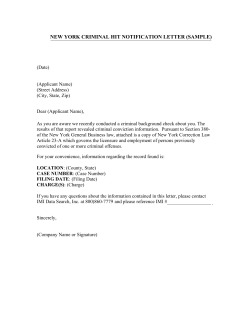


![Dear [Candidate]: Thank you for your willingness to stand for](http://cdn1.abcdocz.com/store/data/001026053_1-7f0c5dc0a9066cdd4178856527c082aa-250x500.png)


© Copyright 2026