1. No category

RNA Sequencing Analysis With TopHat
Booklet
FOR RESEARCH USE ONLY
Overview
2
Sequencing Considerations
6
Converting Base Calls
7
Aligning Reads with TopHat
15
Calling SNPs
22
Detecting Transcripts and Counting
25
Visualizing Results in IGV
32
References
36
Page 1
Overview
Page 2
Overview
This document explains the analysis steps that need to be taken to align reads to a
genome using TopHat. The following steps are explained:
• Sequencing Considerations, 6. This section highlights considerations for generating
the raw sequencing data for RNA Sequencing on the HiSeq 2000, GAIIx , GAIIe, or
HiScan-SQ.
• Converting Base Calls, 7. This section explains how to convert per cycle BCL base
call files into the FASTQ format.
• Aligning Reads with TopHat, 15. This section explains how to align the reads to a
genome using TopHat.
• Calling SNPs, 22. This section explains how to call SNPs using SAMtools pileup and
BEDTools.
• Detecting Transcripts and Counting, 25. This section explains how to identify
transcripts and measure their expression using Cufflinks.
• Visualizing Results in IGV, 32. This section explains visualization and analysis of
the data using the Integrative Genomics Viewer (IGV).
While this document provides detailed instructions, it is not intended to be a
comprehensive guide. Also note that TopHat is not an Illumina supported product, but
an open source initiative. Our goal with this document is to help you run RNA
sequencing analysis using TopHat.
BCL Conversion
The standard sequencing output for the HiSeq2000 consists of *.bcl files, which contain
the base calls and quality scores for per cycle. To convert *.bcl files into fastq.gz files, use
the BCL Converter in CASAVA v1.8.
Bowtie
Bowtie1 is an ultrafast, memory-efficient aligner designed for quickly aligning large sets
of short reads to large genomes. Bowtie indexes the genome to keep its memory footprint
small: for the human genome, the index is typically about 2.2 GB for single-read
alignment or 2.9 GB for paired-end alignment. Multiple processors can be used
simultaneously to achieve greater alignment speed.
Bowtie forms the basis for other tools like TopHat, a fast splice junction mapper for RNAseq reads, and Cufflinks, a tool for transcriptome assembly and isoform quantitiation
from RNA-seq reads.
TopHat
TopHat2 is a fast splice junction mapper for RNA-Seq reads. It aligns RNA-Seq reads to
mammalian-sized genomes using the ultra high-throughput short read aligner Bowtie,
and then analyzes the mapping results to identify splice junctions between exons.
TopHat is a collaborative effort between the University of Maryland Center for
Part # 15024169 C
Unbranded
Overview
Page 3
Bioinformatics and Computational Biology and the University of California, Berkeley
Departments of Mathematics and Molecular and Cell Biology.
Samtools Pileup and Bedtools
As with DNA sequencing data, we can use the RNA sequencing reads to identify SNPs
using the publicly available packages SAMtools and BEDTools. First, the SAMtools
pileup command is used to call SNPs. Next, the BEDTools package filters those SNPs
that are located near splice junctions, since these are often false SNPs.
Cufflinks
Cufflinks3 assembles transcripts, estimates their abundances, and tests for differential
expression and regulation in RNA-Seq samples. It accepts aligned RNA-Seq reads and
assembles the alignments into a parsimonious set of transcripts. Cufflinks then estimates
the relative abundances of these transcripts based on how many reads support each one.
Cufflinks is a collaborative effort between the Laboratory for Mathematical and
Computational Biology, led by Lior Pachter at UC Berkeley, Steven Salzberg's group at the
University of Maryland Center for Bioinformatics and Computational Biology, and
Barbara Wold's lab at Caltech.
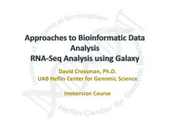
Workflow
The workflow contains the following steps:
Part # 15024169 C Unbranded
Overview
Page 4
Figure 1
Workflow for RNA Sequencing Analysis with TopHat
Installation
This workflow requires installation of the following tools:
• Bowtie (http://bowtie-bio.sourceforge.net)
• TopHat (http://tophat.cbcb.umd.edu/)
• Cufflinks (http://cufflinks.cbcb.umd.edu/)
• SAMtools 0.1.8 (http://samtools.sourceforge.net/)
Part # 15024169 C
Unbranded
Overview
Page 5
• BEDtools 2.15.0 (http://code.google.com/p/bedtools/)
See the “Getting started” link on each webpage referenced above for instructions on
installing each of these tools. The following versions of these packages were used in
developing this workflow, 0.12.7 (Bowtie), v1.4.1 (TopHat), and v1.3.0 (Cufflinks). In
addition to these tools, this workflow also assumes the availability of the following
command-line tools: perl, gunzip, wget, and awk.
Testing the Installation
If you wish to run TopHat and Cufflinks on the command-line, check that each of these
tools has been properly installed by executing the following commands:
• Bowtie:
>bowtie --version
This should return something similar to the following:
bowtie version 0.12.7
64-bit
Built on sd-qmaster.illumina.command-line
Mon Feb 8 14:03:53 PST 2010
Compiler: gcc version 4.1.2 20080704 (Red Hat 4.1.2-44)
Options: -O3
Sizeof {int, long, long long, void*, size_t, off_t}: {4, 8, 8,
8, 8, 8}
• TopHat:
>tophat --version
This should return something similar to the following:
TopHat v1.4.1
…
• Cufflinks:
>cufflinks
This should return something similar to the following:
Cufflinks v1.3.0
…
Verify that there are no errors. If any of these commands generate an error, please check
your installation.
Part # 15024169 C Unbranded
Sequencing Considerations
Page 6
Sequencing Considerations
Library construction:
• Keep track of your mate pair distance: this value is required for the later analysis.
• You can use multiplexed samples. If performing analysis on multiplexed samples,
run the demultiplexing script beforehand, as described by the CASAVA
documentation.
• TopHat deals well with short insert paired-end data. Recommended insert size is
~300bp and it may not be beneficial to create mate pair library with longer (>3 kb)
insert size.
Flow cell generation:
• This workflow supports paired-end reads. You would expect this to help in the
identification of splice junctions.
Sequencing:
• The sequencing coverage depends on what you want to be able to detect. For testing
purposes, we have been using one lane of HiSeq (~80 million reads) for a single
human sample.
• TopHat works well with read length >50bp, the software is optimized for reads 75bp
or longer.
• TopHat can align reads that are up to 1024 bp, and it handles paired end reads, but
we do not recommend mixing several "types" of reads in the same TopHat run.
Part # 15024169 C
Unbranded
Converting Base Calls
Page 7
Converting Base Calls
The standard sequencing output for the HiSeq™ , Genome Analyzer, and RTA v1.13
consists of *.bcl files, which contain the base calls and quality scores per cycle. TopHat
uses .fastq.gz files as input. To convert *.bcl files into .fastq.gzfiles, use CASAVA v1.8.
In addition to generating FASTQ files, CASAVA uses a user-created sample sheet to
divide the run output in projects and samples, and stores these in separate directories. If
no sample sheet is provided, all samples will be put in the Undetermined_Indices
directory by lane, and not demultiplexed. Each directory can be independently analyzed
(alignment, variant analysis, and counting) with CASAVA and contains the files
necessary for alignment, variant analysis, and counting with CASAVA.
At the same time, CASAVA also separates multiplexed samples (demultiplexing).
Multiplexed sequencing allows you to run multiple individual samples in one lane. The
samples are identified by index sequences that were attached to the template during
sample prep. The multiplexed samples are assigned to projects and samples based on the
sample sheet, and stored in corresponding project and sample directories as described
above. At this stage, adapter masking may also be performed. With this feature, CASAVA
will check whether a read has proceeded past the genomic insert and into adapter
sequence. If adapter sequence is detected, the corresponding basecalls will be changed to
N in the resultant FASTQ file.
NOTE
For a comprehensive description of BCL Conversion, see the CASAVA v1.8
User Guide.
Bcl Conversion Input Files
Demultiplexing needs a BaseCalls directory and a sample sheet to start a run. These files
are described below. See also image below.
Part # 15024169 C Unbranded
Converting Base Calls
Page 8
BaseCalls Directory
Demultiplexing requires a BaseCalls directory as generated by RTA or OLB (Off-Line
Basecaller), which contains the binary base call files (*.bcl files).
NOTE
As of 1.8, CASAVA does not use *_qseq.txt files as input anymore.
The BCL to FASTQ converter needs the following input files from the BaseCalls directory:
• *.bcl files.
• *.stats files.
• *.filter files.
Part # 15024169 C
Unbranded
Converting Base Calls
Page 9
• *.control files
• *.clocs, *.locs, or *_pos.txt files. The BCL to FASTQ converter determines which type
of position file it looks for based on the RTA version that was used to generate them.
• RunInfo.xml file. The RunInfo.xml is at the top level of the run folder.
• config.xml file
RTA is configured to copy these files off the instrument computer machine to the
BaseCalls directory on the analysis server.
Generating the Sample Sheet
The user generated sample sheet (SampleSheet.csv file) describes the samples and
projects in each lane, including the indexes used. The sample sheet should be located in
the BaseCalls directory of the run folder. You can create, open, and edit the sample sheet
in Excel.
The sample sheet contains the following columns:
Column
Header
FCID
Lane
SampleID
SampleRef
Index
Description
Flow cell ID
Positive integer, indicating the lane number (1-8)
ID of the sample
The reference used for alignment for the sample
Index sequences. Multiple index reads are separated by a hyphen (for example,
ACCAGTAA-GGACATGA).
Description
Description of the sample
Control
Y indicates this lane is a control lane, N means sample
Recipe
Recipe used during sequencing
Operator
Name or ID of the operator
SampleProject The project the sample belongs to
You can generate it using Excel or other text editing tool that allows .csv files to be saved.
Enter the columns specified above for each sample, and save the Excel file in the .csv
format. If the sample you want to specify does not have an index sequence, leave the
Index field empty.
Illegal Characters
Project and sample names in the sample sheet cannot contain illegal characters not
allowed by some file systems. The characters not allowed are the space character and the
following:
? ( ) [ ] / \ = + < > : ; " ' , * ^ | & .
Multiple Index Reads
If multiple index reads were used, each sample must be associated with an index
sequence for each index read. All index sequences are specified in the Index field. The
individual index read sequences are separated with a hyphen character (-). For example,
if a particular sample was associated with the sequence ACCAGTAA in the first index
read, and the sequence GGACATGA in the second index read, the index entry would be
ACCAGTAA-GGACATGA.
Part # 15024169 C Unbranded
Converting Base Calls
Page 10
Samples Without Index
As of CASAVSA 1.8, you can assign samples without index to projects, sampleIDs, or
other identifiers by leaving the Index field empty.
Running Bcl Conversion and Demultiplexing
Bcl conversion and demultiplexing is performed by one script, configureBclToFastq.pl.
This section describes how to perform Bcl conversion and demultiplexing in CASAVA
1.8.
Usage of configureBclToFastq.pl
The standard way to run bcl conversion and demultiplexing is to first create the
necessary Makefiles, which configure the run. Then you run make on the generated files,
which executes the calculations.
1
Enter the following command to create a makefile for demultiplexing:
/path-to-CASAVA/bin/configureBclToFastq.pl[options]
NOTE
The options have changed significantly between CASAVA 1.7 and 1.8. See
Options for Bcl Conversion and Demultiplexing, 10.
2
Move into the newly created Unaligned folder specified by --output-dir.
3
Type the “make” command. Suggestions for “make” usage, depending on your
workflow, are listed below.
Make Usage
nohup make -j N
nohup make -j N r1
Workflow
Bcl conversion and demultiplexing (default).
Bcl conversion and demultiplexing for read 1.
See Makefile Options for Bcl Conversion and Demultiplexing, 12 for explanation of
the options.
NOTE
The ALIGN option, which kicked off configureAlignment after demultiplexing
was done in CASAVA 1.7, is no longer available.
4
After the analysis is done, review the analysis for each sample.
Options for Bcl Conversion and Demultiplexing
The options for demultiplexing are described below.
Option
--fastq-cluster-count
-i, --input-dir
Description
Maximum number of clusters per output
FASTQ file. Do not go over 16000000, since this
is the maximum number of reads we
recommend for one ELAND process. Specify 0
to ensure creation of a single FASTQ file.
Defaults to 4000000.
Path to a BaseCalls directory.\
Defaults to current dir
Examples
--fastq-clustercount 6000000
--input-dir
<BaseCalls_dir>
Part # 15024169 C
Unbranded
Converting Base Calls
Page 11
Option
-o, --output-dir
--positions-dir
--positions-format
--filter-dir
--intensities-dir
-s,--sample-sheet
--tiles
--use-bases-mask
--no-eamss
--mismatches
Part # 15024169 C Unbranded
Description
Path to demultiplexed output.
Defaults to <run_folder>/Unaligned
Note that there can be only one Unaligned
directory by default. If you want multiple
Unaligned directories, you will have to use this
option to generate a different output directory.
Path to a directory containing positions files.
Defaults depends on the RTA version that is
detected.
Format of the input cluster positions
information. Options:
• .locs
• .clocs
• _pos.txt
Defaults to .clocs.
Path to a directory containing filter files.
Defaults depends on RTA version that is
detected.
Path to a valid Intensities directory.
Defaults to parent of base_calls_dir.
Path to sample sheet file.
Defaults to <input_dir>/SampleSheet.csv
Examples
--output-dir <run_
folder>/Unaligned
--positions-dir
<positions_dir>
--positions-format
.locs
--filter-dir
<filter_dir>
--intensities-dir
<intensities_dir>
--sample-sheet
<input_
dir>/SampleSheet.csv
--tiles=s_[2468]_[0--tiles option takes a comma-separated list of
9][0-9][02468]5,s_1_
regular expressions to match against the
expected "s_<lane>_<tile>" pattern, where <lane> 0001
is the lane number (1-8) and <tile> is the 4 digit
tile number (left-padded with 0s).
The --use-bases-mask string specifies how to --use-bases-mask
y50n,I6n,Y50n
use each cycle.
This means:
• An “n” means ignore the cycle.
• Use first 50 bases for
• A “Y” (or "y") means use the cycle.
first read (Y50)
• An “I” means use the cycle for the index
• Ignore the next (n)
read.
• Use 6 bases for index
• A number means that the previous
(I6)
character is repeated that many times.
• The read masks are separated by commas ", • Ignore next (n)
"
• Use 50 bases for second
read (Y50)
The format for dual indexing is as follows:-use-bases-mask Y*,I*,I*,Y* or variations • Ignore next (n)
thereof as specified above.
If this option is not specified, the mask will be
determined from the 'RunInfo.xml' file in the
run directory. If it cannot do this, you will have
to supply the --use-bases-mask.
Disable the masking of the quality values with --no-eamss
the Read Segment Quality control metric filter.
Comma-delimited list of number of mismatches --mismatches 1
allowed for each read (for example: 1,1). If a
single value is provide, all index reads will allow
the same number mismatches.
Default is 0.
Converting Base Calls
Page 12
Option
--flowcell-id
--ignore-missing-stats
--ignore-missing-bcl
--ignore-missingcontrol
--with-failed-reads
--adapter-sequence
--man
-h, --help
Description
Use the specified string as the flowcell id.
(default value is parsed from the config-file)
Fill in with zeros when *.stats files are missing
Examples
--flowcell-id flow_
cell_id
--ignore-missingstats
--ignore-missing-bcl
Interpret missing *.bcl files as no call
Interpret missing control files as not-set control --ignore-missingcontrol
bits
--with-failed-reads
Include failed reads into the FASTQ files (by
default, only reads passing filter are included).
Path to a FASTA adapter sequence file. If there --adapter-sequence
<adapter
are two adapters sequences specified in the
FASTA file, the second adapter will be used to dir>/adapter.fa
mask read 2. Else, the same adapter will be used
for all reads.
Default: None (no masking)
--man
Print a manual page for this command
-h
Produce help message and exit
Makefile Options for Bcl Conversion and Demultiplexing
The options for make usage in demultiplexing/analysis are described below.
Parameter
nohup
Description
Use the Unix nohup command to redirect the standard output and keep the “make”
process running even if your terminal is interrupted or if you log out. The standard output
will be saved in a nohup.out file and stored in the location where you are executing the
makefile.
nohup make -j n &
The optional “&” tells the system to run the analysis in the background, leaving you free
to enter more commands.
We suggest always running nohup to help troubleshooting if issues arise.
-j N
The -j option specifies the extent of parallelization, with the options depending on the
setup of your computer or computing cluster.
r1
Runs Bcl conversion for read 1. Can be started once the last read has started sequencing.
POST_RUN_
A Makefile variable that can be specified either on the make command line or as an
COMMAND_R1 environment variable to specify the post-run commands after completion of read one, if
needed. Typical use would be triggering the alignment of read 1.
POST_RUN_
A Makefile variable that can be specified on the make command line to specify the postCOMMAND
run commands after completion of the run.
KEEP_
The option KEEP_INTERMEDIARY tells the software not to delete the intermediary files in
INTERMEDIARY the Temp dir after Bcl conversion is complete. Usage: KEEP_INTERMEDIARY:=yes
NOTE
If you specify one of the more specific workflows and then run a more
general one, only the difference will get processed. For instance:
make -j N r1
followed by:
make -j N
will do read 1 in the first step, and read 2 the second one.
Part # 15024169 C
Unbranded
Converting Base Calls
Page 13
Bcl Conversion Output Folder
The Bcl Conversion output directory has the following characteristics:
• The project and sample directory names are derived from the sample sheet.
• The Demultiplex_Stats file shows where the sample data are saved in the directory
structure.
• The Undetermined_indices directory contains the reads with an unresolved or
erroneous index.
• If no sample sheet exists, the software generates a project directory named after the
flow cell, and sample directories for each lane.
• Each directory is a valid base calls directory that can be used for subsequent
alignment analysis.
NOTE
If the majority of reads end up in the 'Undetermined_indices' folder, check the
--use-bases-mask parameter syntax and the length of the index in the sample
sheet. It may be that you need to set the --use-bases-mask option to the
length of the index in the sample sheet + the character 'n' to account for
phasing. Note that you will not be able to see which indices have been placed
in the 'Undetermined_indices' folder
Part # 15024169 C Unbranded
Converting Base Calls
Page 14
NOTE
There can be only one Unaligned directory by default. If you want multiple
Unaligned directories, you will have to use the option --output-dir to
generate a different output directory.
Part # 15024169 C
Unbranded
Aligning Reads with TopHat
Page 15
Aligning Reads with TopHat
TopHat is a short-read aligner specifically designed for alignment of RNA sequencing
data. It is built on top of the Bowtie aligner, aligning to both the genome and splice
junctions without a reference splice site annotation.
This section will walk you through the following tasks:
• Aligning a set of RNA reads against a genome without an annotated set of splice
boundaries.
Generating a Workflow Directory
Before starting the alignment, create a directory to contain the results of this workflow:
>mkdir <WorkflowFolder>
>cd <WorkflowFolder>
Where:
• <WorkflowFolder> is the path and folder where the results should be stored.
Workflow Folder Custom Examples and Comments
TopHat Input Files
TopHat uses the following input files:
• Reads in FASTQ format. You can use the compressed FASTQ files produced by the
BCL converter supplied with CASAVA 1.8 (configureBclToFastq.pl).
• Genome files in a special indexed format (ebwt).
• You can also use the reference annotation, if available.
Read Files Custom Examples and Comments
Part # 15024169 C Unbranded
Aligning Reads with TopHat
Page 16
Genome Reference Files
To provide TopHat with genome files, you need to do the following:
1
Generate a Genomes folder
2
Obtain a genome against which to align your reads. You can use the genomes
available from Illumina, or any genome FASTA file.
3
Convert the FASTA genome files to a special indexed format (ebwt) using a tool
provided with the Bowtie build.
Illumina Provided Genomes
Illumina provides a number of commonly used genomes at ftp.illumina.com along with
a reference annotation:
• Arabidopsis_thaliana
• Bos_taurus
• Caenorhabditis_elegans
• Canis_familiaris
• Drosophila_melanogaster
• Equus_caballus
• Escherichia_coli_K_12_DH10B
• Escherichia_coli_K_12_MG1655
• Gallus_gallus
• Homo_sapiens
• Mus_musculus
• Mycobacterium_tuberculosis_H37RV
• Pan_troglodytes
• PhiX
• Rattus_norvegicus
• Saccharomyces_cerevisiae
• Sus_scrofa
You can login using the following credentials:
• Username: igenome
• Password: G3nom3s4u
For example, download the FASTA, annotation, and bowtie index files for the human
hg18 genome from the iGenomes repository with the following commands:
>wget --ftp-user=igenome --ftp-password=G3nom3s4u
ftp://ftp.illumina.com/Homo_sapiens/UCSC/hg18/Homo_sapiens_
UCSC_hg18.tar.gz
Unpack the tar file:
tar xvzf Homo_sapiens_UCSC_hg18.tar.gz
Unpacking will make its own folder
Homo_sapiens/UCSC/hg18
Within this folder, the following files are present:
Homo_sapiens/UCSC/hg18/Annotation/Genes/genes.gtf
Part # 15024169 C
Unbranded
Aligning Reads with TopHat
Page 17
Homo_sapiens/UCSC/hg18/Sequence/BowtieIndex/genome*.*
Genome Build Custom Examples and Comments
Custom Genome Files
If you are providing your own reference annotation, please note that it must be in GTF
format (http://mblab.wustl.edu/GTF22.html). In addition, the chromosome names must
match the chromosome names specified in the FASTA genome files.
Library Type
In the analysis of RNA-seq data, both TopHat and Cufflinks can take into account the
nature of the sample preparation. Specifically, the analysis can specify that the sequenced
fragments are either:
• Unstranded
• Correspond to the first strand
• Correspond to the second strand
For the TruSeq RNA Sample Prep Kit, the appropriate library type is "fr-unstranded". For
TruSeq stranded sample prep kits, the library type is specified as "fr-firststrand".
Single-Read Alignment
The next section provides instructions for the single-read alignment workflow in TopHat.
I f you want to do paired-end alignment, see Paired-End Alignment, 19
Single Read Test Data
Two sample sets of single 75 base pair reads are available for use as test data with this
workflow. These sets are from two different tissues (UHR and brain). To get this data,
perform the following:
1
Download both of these files to the workflow directory (the current directory):
>wget --ftp-user=RNASeq --ftp-password=illumina
ftp://ftp.illumina.com/UHR.tgz
>wget --ftp-user=RNASeq --ftp-password=illumina
ftp://ftp.illumina.com/brain.tgz
2
Extract the archive files,
>tar xvzf UHR.tgz
>tar xvzf brain.tgz
Part # 15024169 C Unbranded
Aligning Reads with TopHat
Page 18
These commands create two directories, “UHR” and “brain” in the current directory,
containing fastq.gz files much like the sample directories that would be produced by the
BCL converter in CASAVA v1.8.
Generating Single-Read FASTQ Files
Before alignment with TopHat, fastq.gz input files must be uncompressed. For every
folder with fastq.gz files, perform the following:
>gunzip -c <DataFolder>/*.gz > <SampleID>.fastq
Where:
• <DataFolder> is the path and folder where a set of reads (one sample) is stored
• <SampleID> is the name of the sample being converted
Test Data
For example, for the test data, this would be the following:
>gunzip -c UHR/*.gz > UHR.fastq
>gunzip -c brain/*.gz > brain.fastq
Running Single Read Alignment
Start the single-read alignments for each sample by entering the following command:
>tophat --GTF <iGenomesFolder>/Annotation/Genes/genes.gtf
--library-type <LibraryType> --num-threads 1
--output-dir <SampleOutputFolder>
<iGenomesFolder>/Sequence/BowtieIndex/genome <SampleID>.fastq
Where:
• <SampleOutputFolder> is the path and folder where the sample output will be
stored
• <iGenomesFolder> is the path and folder of the iGenomes directory
• <SampleID> is the name of the sample being converted
• <LibraryType> is the library type correspond to your sample preparation (see
Library Type, 17).
The main option to modify the analysis is the following:
--num-threads If the workflow is run on a machine with multiple cores, this number may
1
be increased to reflect the number of cores present.
Test Data
For example, for the test data, this would be the following:
>tophat --GTF Homo_
sapiens/UCSC/hg18/Annotation/Genes/genes.gtf
--library-type fr-firststrand --num-threads 1
--output-dir UHR_output Homo_
sapiens/UCSC/hg18/Sequence/BowtieIndex/genome UHR.fastq
>tophat --GTF Homo_
sapiens/UCSC/hg18/Annotation/Genes/genes.gtf
--library-type fr-firststrand --num-threads 1
Part # 15024169 C
Unbranded
Aligning Reads with TopHat
Page 19
--output-dir brain_output Homo_
sapiens/UCSC/hg18/Sequence/BowtieIndex/genome brain.fastq
SR Alignment Custom Examples and Comments
Paired-End Alignment
The next section provides instructions for the paired-end alignment workflow in TopHat.
If you want to do paired-end alignment, see Single-Read Alignment, 17
Paired-End Test Data
Two sample sets of 50 base pair paired-end reads are available for use as test data with
this workflow. These sets are from two different tissues (UHR and brain). To get this data,
perform the following:
1
Download both of these files to the workflow directory (the current directory):
>wget --ftp-user=RNASeq --ftp-password=illumina
ftp://ftp.illumina.com/UHR_paired.tgz
>wget --ftp-user=RNASeq --ftp-password=illumina
ftp://ftp.illumina.com/brain_paired.tgz
2
The archive files must first be extracted,
>tar xvzf UHR_paired.tgz
>tar xvzf brain_paired.tgz
These commands create two directories, “UHR” and “brain” in the current directory,
containing fastq.gz files much like those that would be produced by the BCL converter in
CASAVA v1.8.
Generating Paired-End FASTQ Files
Before alignment with TopHat, compressed FASTQ input files must first be
uncompressed. The first and second reads must be placed into separate FASTQ files. For
every folder with compressed FASTQ files, perform the following:
>gunzip -c <DataFolder>/*R1*.gz > <sampleID>_1.fastq
>gunzip -c <DataFolder>/*R2*.gz > <sampleID>_2.fastq
Where:
• <DataFolder> is the path and folder where a set of reads (one sample) is stored
• <sampleID> is the name of the sample being converted
Part # 15024169 C Unbranded
Aligning Reads with TopHat
Page 20
Test Data
For example, for the test data, this would be the following:
>gunzip -c UHR/*R1*.gz > UHR_1.fastq
>gunzip -c brain/*R1*.gz > brain_1.fastq
>gunzip -c UHR/*R2*.gz > UHR_2.fastq
>gunzip -c brain/*R2*.gz > brain_2.fastq
Running Paired-End Alignment
Start the paired-end alignments for each sample by entering the following command:
>tophat --GTF <iGenomesFolder>/Annotation/Genes/genes.gtf
--library-type <LIBRARY_TYPE> --mate-inner-dist 100 --numthreads 1 --output-dir <SampleOutputFolder>
<iGenomesFolder>/Sequence/BowtieIndex/genome <SampleID>_1.fastq
<SampleID>_2.fastq
Where:
• <SampleOutputFolder> is the path and folder where the sample output will be
stored
• <iGenomesFolder> is the path and folder of the iGenomes directory
• <SampleID> is the name of the sample being converted
• <LibraryType> is the library type correspond to your sample preparation (see
Library Type, 17).
The main option to modify the analysis is the following:
--numthreads
1
--mateinnerdist
If the workflow is run on a machine with multiple cores, this number may be
increased to reflect the number of cores present.
In the paired-end alignment, the option --mate-inner-dist specifies the inner distance
between the paired reads. For example, for a sample with insert size of 200 bases
and two reads of 50 bases, this mate-inner-dist parameter would be 100 (total insert
size of 200 minus 2x50 reads).
Test Data
For example, for the test data, this would be the following:
>tophat --GTF Homo_
sapiens/UCSC/hg18/Annotation/Genes/genes.gtf
--library-type fr-firststrand --mate-inner-dist 100 --numthreads 1 --output-dir UHR_output
Homo_sapiens/UCSC/hg18/Sequence/BowtieIndex/genome UHR_1.fastq
UHR_2.fastq
>tophat --GTF Homo_sapiens/UCSC/hg18/Annotation/Genes/genes.gtf
--library-type fr-firststrand --mate-inner-dist 100 --numthreads 1 --output-dir brain_output
Homo_sapiens/UCSC/hg18/Sequence/BowtieIndex/genome brain_
1.fastq brain_2.fastq
Part # 15024169 C
Unbranded
Aligning Reads with TopHat
Page 21
PE Alignment Custom Examples and Comments
TopHat Output Description
Whether executing the single or paired-end alignment, the alignment should create, for
each sample, a new folder within the Workflow folder, for example “UHR_output” and
“brain_output” for the test data. These folders contain the output of each alignment, and
inside each alignment directory, there are several files:
• accepted_hits.bam—This BAM-format file details the mapping of each read to the
genome.
• junctions.bed —This file contains information, including genomic location and
supporting evidence, about all of the splice junctions discovered by TopHat in the
process of aligning reads.
The accepted_hits.bam file is used for further analysis in quantification of transcripts
within the sample.
NOTE
For more information about the BAM format, see
http://samtools.sourceforge.net/
Part # 15024169 C Unbranded
Calling SNPs
Page 22
Calling SNPs
As with DNA sequencing data, we can use the RNA sequencing reads to identify SNPs
using the publicly available packages SAMtools (http://samtools.sourceforge.net/) and
BEDTools (http://code.google.com/p/bedtools/).
Input Files
SNP calling uses the following input files:
• The BAM file from TopHat, containing the mapped locations of the input reads.
These are located in the file accepted_hits.bam in the TopHat output folder for the
sample.
• Genome files.
• The junctions file from TopHat (junctions.bed).
Running Pileup to Identify SNPs
With the alignments in the proper format, it is now possible to call SNPs. This will be
accomplished with the “SAMtools pileup” command. It may be useful to investigate the
options for this command to further tailor the SNP calling to your particular preferences.
Note that the "samtools.pl” command is typically located in the “misc” directory of the
samtools package.
Start the SNP calling for each sample by entering the following command:
samtools mpileup -u -q 10 -f
<iGenomesFolder>/Sequence/WholeGenomeFasta/genome.fa accepted_
hits.bam | bcftools view -g - | vcfutils.pl varFilter | awk '
($6 >= 50)' > <SampleOutputFile>
Where:
• <iGenomesFolder> is the path and folder of the iGenomes build
• <SampleInputBAM> is the path and BAM file that is used as input for pileup
• <SampleOutputFile> is the output path and file
Test Data
For the test data, running pileup would be the following:
samtools mpileup -u -q 10 -f Homo_
sapiens/UCSC/hg18/Sequence/WholeGenomeFasta/genome.fa UHR_
output/accepted_hits.bam | bcftools view -g - | vcfutils.pl
varFilter | awk '($6 >= 50)' > UHR_output/UHR.raw.pileup
samtools mpileup -u -q 10 -f Homo_
sapiens/UCSC/hg18/Sequence/WholeGenomeFasta/genome.fa brain_
output/accepted_hits.bam | bcftools view -g - | vcfutils.pl
varFilter | awk '($6 >= 50)' > brain_output/brain.raw.pileup
Pileup Custom Examples and Comments
Part # 15024169 C
Unbranded
Calling SNPs
Page 23
Running Bedtools to Filter SNPs
Alignments produced by TopHat often induce false SNP calls near splice sites, and the
BEDTools package filters those SNPs out.
1
The first step is to use the junctions.bed file provided by TopHat to create a new bed
file describing a window of 5 base pairs around each splice site junction.
>bowtie-inspect -s <GenomesFolder>/genome.fa | tail -n +4 | cut
-f 2- > genome_size.txt
>cat <JunctionsFile> | bed_to_juncs | flankBed -g genome_
size.txt -b 1 | slopBed -g genome_size.txt -b 5 >
<JunctionsWindowFile>
Where:
• <JunctionsFile> is the path and file that describes the junctions, the TopHat
junctions.bed file
• <JunctionsWindowFile> is the output windows.bed file, with path
2
The “intersectBed” command in the BEDTools package can then be used to identify
SNPs that fall outside of these regions.
>intersectBed -v -wa -a <SampleInputFile> -b
<JunctionsWindowFile> > <SampleOutputFile>
Where:
• <SampleInputFile> is the raw input file generated by pileup, with path
• <JunctionsWindowFile> is the path and file that describes the junctions with
additional window created in step 1
• <SampleOutputFile> is the filtered output .pileup file, with path
NOTE
slopBed and intersectBed are utilities provided by the BEDtools package that
you installed earlier (see Installation, 4).
Test Data
For the test data, generating the windows would be the following:
>bowtie-inspect -s Homo_
sapiens/UCSC/hg18/Sequence/BowtieIndex/genome | tail -n +4 |
cut -f 2- > genome_size.txt
>cat UHR_output/junctions.bed | bed_to_juncs | flankBed -g
genome_size.txt -b 1 | slopBed -g genome_size.txt -b 2 > UHR_
output/windows.bed
>cat brain_output/junctions.bed | bed_to_juncs | flankBed -g
genome_size.txt -b 1 | slopBed -g genome_size.txt -b 2 > brain_
output/windows.bed
Part # 15024169 C Unbranded
Calling SNPs
Page 24
The “intersectBed” command would be like this:
>intersectBed -v -wa -a UHR_output/UHR.raw.pileup -b UHR_
output/windows.bed > UHR_output/UHR.filtered.pileup
>intersectBed -v -wa -a brain_output/brain.raw.pileup -b brain_
output/windows.bed > brain_output/brain.filtered.pileup
Window and IntersectBed Custom Examples and Comments
Output Description
The files UHR.filtered.pileup and brain.filtered.pileup now contain the list of filtered SNP
calls in SAM pileup format.
Part # 15024169 C
Unbranded
Detecting Transcripts and Counting
Page 25
Detecting Transcripts and Counting
At this stage, the SAM file from TopHat only contains the mapped locations of the input
reads. Cufflinks is a suite of tools for quantifying aligned RNA sequencing data. The
Cufflinks suite assembles these reads into transcripts, as well as quantifies these
transcripts in single or multiple experiments.
The Cufflinks suite has three separate tools (cufflinks, cuffmerge, and cuffdiff) for the
following tasks:
• Cufflinks—assembles novel transcripts AND quantifies transcripts against a given
annotation.
• Cuffmerge—takes novel transcripts from multiple experiments and combines them
into one annotation file.
• Cuffdiff—calculates differential expression given an annotation file; does not need or
use the quantification information from cufflinks.
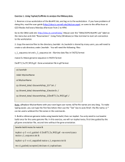
The workflow for running the Cufflinks suite is illustrated below.
Figure 1
Part # 15024169 C Unbranded
Cufflinks Workflow
Detecting Transcripts and Counting
Page 26
NOTE
The second cufflinks step is optional. It generates the transcripts.expr and genes.expr files
that provide a good summary of the expression values.
Detecting Transcripts and Counting Input Files
Cufflinks uses the following input files:
• The BAM file from TopHat, containing the mapped locations of the input reads.
These are located in the file accepted_hits.bam in the TopHat output folder for the
sample.
• Optional: reference annotation, if available, to quantify expression of known
transcripts.
Identifying Novel Transcripts
If you wish to identify novel transcripts (optional), you need to perform the following two
commands:
• First use cufflinks to assemble novel transcripts from the aligned reads.
• Use cuffmerge to combine the list of transcripts from the two alignments, as well as
map these transcripts against a reference annotation.
Running Cufflinks
Run cufflinks by entering the following commands for each sample:
>cd <OutputFolder>
>cufflinks --library-type <LibraryType> --GTF-guide
<iGenomeFolders>/Annotation/Genes/genes.gtf
--label <SampleID> --num-threads 1 accepted_hits.bam
>cd ..
Where:
• <OutputFolder> is the path and folder where the TopHat output is stored
• <LibraryType> is the library type correspond to your sample preparation (see
Library Type, 17).
• <SampleID> is the name of the sample being converted
• <iGenomesFolder> is the downloaded iGenomes directory
The main option to modify the analysis is the following:
--num-threads 1 If the workflow is run on a machine with multiple
cores, this number may be increased to reflect the
number of cores present.
Test Data
For example, for the test data, this would be the following:
>cd UHR_output
>cufflinks --library-type fr-firststrand --GTF-guide ../Homo_
sapiens/UCSC/hg18/Annotation/Genes/genes.gtf
--label UHR --num-threads 1 accepted_hits.bam
Part # 15024169 C
Unbranded
Detecting Transcripts and Counting
Page 27
>cd ../brain_output
>cufflinks --library-type fr-firststrand --GTF-guide ../Homo_
sapiens/UCSC/hg18/Annotation/Genes/genes.gtf
--label brain --num-threads 1 accepted_hits.bam
>cd ..
Cufflinks Custom Examples and Comments
Cufflinks Output
In each output directory, this will create several files,
• transcripts.gtf—This file contains the assembled transcripts. You can view the gtf file
of all cufflinks transcripts directly in genome browsers such as the broad IGV or
UCSC browser, which could be useful for visual comparison with known
annotations. For further description of the format and contents of this file, see
http://cufflinks.cbcb.umd.edu/manual.html.
Comparing Transcripts
Cuffmerge can be used to combine the list of transcripts from the two alignments, as well
as map these transcripts against a reference annotation.
Running Cuffmerge
In order to run cuffmerge, the list of transcripts to merge must first be written to a text
file. The following command instructs cuffmerge to compare the assembled transcripts
from different samples, and annotate the result using the annotation GTF file.
>cuffmerge -o <OutputDir>
-g <iGenomesFolder>/Annotation/Genes/genes.gtf
<assembly_GTF_list.txt>
Where:
• <iGenomesFolder> is the downloaded iGenomes directory..
• <OutputDir> is the directory to contain the cuffmerge output
• <assembly_GTF_list.txt> is a text file listing the input GTF files to be merged.
The main options to modify the analysis are the following:
-o <Output
Directory>
-g
Part # 15024169 C Unbranded
Directory where merged assembly will be written
An optional "reference" annotation GTF. Each sample
is matched against this file, and sample isoforms are
tagged as overlapping, matching, or novel where
appropriate.
Detecting Transcripts and Counting
Page 28
Test Data
For example, for the test data, this would be the following:
>echo "UHR_output/transcripts.gtf" > assembly_GTF_list.txt
>echo "brain_output/transcripts.gtf" >> assembly_GTF_list.txt
>cuffmerge -o CuffMerge_Output -g Homo_
sapiens/UCSC/hg18/Annotation/Genes/genes.gtf assembly_GTF_
list.txt
Cuffmerge Custom Examples and Comments
Cuffmerge Output
Several files will be generated in the specified output directory:
• isoforms.fpkm_tracking
• The merged.gtf file provides the set of merged transcripts. Each line contains an
annotation field (“class_code”) that describes the nature of the overlap of this
transcript with transcripts from the reference annotation. The table below, taken from
the cufflinks manual (http://cufflinks.cbcb.umd.edu/manual.html), provides a
description of the possible class codes.
=
c
j
e
Match
Contained
New isoform
A single exon transcript overlapping a reference exon and at least 10 bp of a reference intron,
indicating a possible pre-mRNA fragment
i A single exon transcript falling entirely with a reference intron
r Repeat, currently determined by looking at the reference sequence and applied to transcripts
where at least 50% of the bases are lower case
p Possible polymerase run-on fragment
u Unknown, intergenic transcript
o Unknown, generic overlap with reference
. Tracking file only, indicates multiple classifications
Transcripts annotated with the ‘c’, ‘i’, ‘j’, ‘u’, or ‘o’ class codes represent novel transcripts
of potential interest.
For the remainder of the workflow, you can use the merged annotation file merged.gtf
instead of the reference annotation.
Part # 15024169 C
Unbranded
Detecting Transcripts and Counting
Page 29
Quantifying Genes and Transcripts
If cufflinks is provided an annotation GTF file, it will quantify the genes and transcripts
specified in that annotation, ignoring any alignments that are incompatible with those
annotations. Run cufflinks with an annotation file for all samples:
>cd <SampleOutputFolder>
>cufflinks --library-type fr-firststrand --num-threads 1 -G
<iGenomesFolder>/Annotation/Genes/genes.gtf accepted_hits.bam
>cd ..
Where:
• <LibraryType> is the library type correspond to your sample preparation (see
Library Type, 17).
• <SampleOutputFolder> is the path and folder where the sample output will be
stored
• <iGenomesFolder> is the path and folder where the genome is stored
WARNING
If you run cufflinks in the directory where there is already output from
another cufflinks it will be over-written. If you want to keep different cufflinks
outputs run each cufflinks from different directory as it always prints output
in current directory.
The main options to modify the analysis are the following:
--num-threads 1 If the workflow is run on a machine with multiple cores,
this number may be increased to reflect the number of
cores present.
-G
Tells Cufflinks to use the supplied reference annotation to
estimate isoform expression. It will not assemble novel
transcripts, and the program will ignore alignments not
structurally compatible with any reference transcript.
Test Data
For example, for the test data, this would be the following:
>cd UHR_output
>cufflinks --library-type fr-firststrand --num-threads 1 -G
../Homo_sapiens/UCSC/hg18/Annotation/Genes/genes.gtf accepted_
hits.bam
>cd ..
>cd brain_output
>cufflinks --library-type fr-firststrand --num-threads 1 -G
../Homo_sapiens/UCSC/hg18/Annotation/Genes/genes.gtf accepted_
hits.bam
>cd ..
Part # 15024169 C Unbranded
Detecting Transcripts and Counting
Page 30
Quantifying Custom Examples and Comments
Quantification Output
In each output directory, this will create two output files:
• genes.fpkm_tracking, quantifying the expression of genes, specified in the GTF
annotation file.
• isoforms.fpkm_tracking, quantifying the expression of transcripts, specified in the
GTF annotation file.
Expression is reported in terms of FPKM, or Fragments Per Kilobase of sequence per
Million mapped reads. In simple terms, this measure normalizes the number of aligned
reads by the size of the sequence feature and the total number of mapped reads.
Differential Expression
Cuffdiff will perform a differential expression analysis between two samples on
annotated genes. Run cuffdiff, providing a GTF file and the two SAM-format alignment
files, the following way:
>cuffdiff --library-type fr-firstrand --library-type
<LibraryType> -L <sample list> -o <OutputDir>
<iGenomesFolder>/Annotation/Genes/genes.gtf
<SampleOutputFolder1>/accepted_hits.bam
<SampleOutputFolder2>/accepted_hits.bam
Where:
• <LibraryType> is the library type correspond to your sample preparation (see
Library Type, 17).
• <SampleOutputFolder1> and <SampleOutputFolder2> are the paths and folders
where the two SAM-format alignment files are stored
• <SampleList> is a comma-delimited list of labels for the samples
• <iGenomesFolder> is the path and folder where the genome is stored
• <OutputDir> is the location to store output files
Test Data
For example, for the test data, this would be the following:
>cuffdiff -L UHR,brain -o CuffDiff_Output
Homo_sapiens/UCSC/hg18/Annotation/Genes/genes.gtf UHR_
output/accepted_hits.bam brain_output/accepted_hits.bam
This command will create several files in the specified output directory. The merged GTF
created by cuffmerge may be used instead of the GTF file supplied with iGenomes. The
expression of both genes and specific isoforms are directly compared in the files “gene_
Part # 15024169 C
Unbranded
Detecting Transcripts and Counting
Page 31
exp.diff” and “isoform_exp.diff.” For a discussion of other files generated by this
command, please see the manual at http://cufflinks.cbcb.umd.edu/manual.html.
Cuffdiff Custom Examples and Comments
Part # 15024169 C Unbranded
Visualizing Results in IGV
Page 32
Visualizing Results in IGV
Integrative Genomics Viewer (IGV; http://www.broadinstitute.org/igv/) can be used to
visualize the results of the RNA sequencing results. This part of the workflow will
describe how to visualize the alignments, junction counts, and gene models. coverage.wig
and junctions.bed can be used for immediate visualization of the TopHat alignments as
custom tracks in the IGV.
IGV Input Files
IGV uses the following input files:
• Junctions counts (junctions.bed).
• Gene models in GTF format.
• Alignment files in BAM format.
Some of the TopHat output files should be slightly modified for better visualization; this
is described below.
Indexing BAM Files
The BAM files must be indexed to view in IGV:
>samtools index <SampleInputSortedBAM>
Where:
• <SampleInputBAM> is the sorted BAM file that needs to be indexed (with .bam
extension)
NOTE
SAM/BAM file visualization is useful only at read alignment level. When
zooming out, you will see no coverage.
To view overall coverage across a chromosome, upload coverage.wig. Please
note that starting TopHat v1.1. there is no coverage.wig file produced. Use
IGVtools or BEDTools to make the coverage track from the BAM file.
Test Data
For the test data, indexing would be the following:
>samtools index UHR_output/accepted_hits.bam
>samtools index brain_output/accepted_hits.bam
Indexing BAM Files Custom Examples and Comments
Part # 15024169 C
Unbranded
Visualizing Results in IGV
Page 33
Junction Counts
In each alignment directory, the file junctions.bed contains the number of reads aligned to
each intron junction. While it is possible to immediately load this file into IGV, we will
first make a few useful modifications, including adding a track name and replacing the
TopHat identifier with the number of supporting reads. This is accomplished with the
following command:
>echo "track name=<SampleID> description=\"<SampleID>\"" >
<SampleOutputFolder>/modified_junctions.bed
>tail -n +2 <SampleOutputFolder>/junctions.bed | perl -lane
'print join("\t",(@F[0..2,4],$F[4]*50,@F[5..$#F]))' >>
<SampleOutputFolder>/modified_junctions.bed
Where:
• <SampleID> is the prefix for the output
• <SampleOutputFolder> is the path and folder where the output is stored of the
samples being compared
Test Data
For example, for the test data, this would be the following:
>echo "track name=UHRJunctions description=\"UHR Junctions\"" >
UHR_output/modified_junctions.bed
>tail -n +2 UHR_output/junctions.bed | perl -lane 'print join
("\t",(@F[0..2,4],$F[4]*50,@F[5..$#F]))' >> UHR_
output/modified_junctions.bed
>echo "track name=brainJunctions description=\"Brain
Junctions\"" > brain_output/modified_junctions.bed
>tail -n +2 brain_output/junctions.bed | perl -lane 'print join
("\t",(@F[0..2,4],$F[4]*50,@F[5..$#F]))' >> brain_
output/modified_junctions.bed
JunctionsFile Custom Examples and Comments
Gene Models
The gene models in GTF format can be directly visualized by IGV.
Especially if you have elected to identify novel transcripts, the GTF file may be quite large
and require a great deal of memory to visualize in IGV.If necessary, you may create a
chromosome specific gene-model file to conserve memory. For example, assuming that
Part # 15024169 C Unbranded
Visualizing Results in IGV
Page 34
chromosome 22 is annotated as “chr22” in your genome, you could create a pared-down
GTF file containing only chromosome 22 with the following command,
>cat Homo_sapiens/UCSC/hg18/Annotation/Genes/genes.gtf | grep
“^chr22” > Homo_sapiens/UCSC/hg18/Annotation/geneschromosome22.gtf
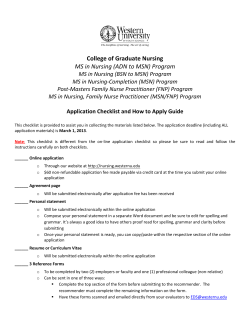
IGV Visualization
Load each of the output files generated above with the IGV browser
(http://www.broadinstitute.org/igv/). Note that if you are copying the result files to an
alternate computer for visualization, you must copy the alignment index
(<SampleID>.bam.bai files), as well as the alignment itself (<SampleID>.bam). Loading
these values will produced the following visualization, allowing you to see coverage,
aligned reads, and junction counts for each of the two tissues.
You may also want to upload the GTF file for the transcripts model, along with a
junction track that shows the number of reads supporting each junction and a
comparison to a known annotation track (for example, the Refseq transcripts in
broadIGV). This will help you compare your data to known transcripts and see
differences between different samples.
NOTE
For large genome regions we recommend uploading separate coverage track
as BAM coverage is shown only for smaller regions. Also please aware that
loading a full BAM file for large regions with very highly expressed transcript
may kill or freeze the browser.
Part # 15024169 C
Unbranded
Visualizing Results in IGV
Page 35
Figure 1
Samples Viewed in the IGV Browser
Part # 15024169 C Unbranded
References
Page 36
References
1
Langmead B, Trapnell C, Pop M, Salzberg SL. (2009) Ultrafast and memory-efficient
alignment of short DNA sequences to the human genome. Genome Biol 10(3):R25.
2
Trapnell C, Pachter L, Salzberg SL.(2009) TopHat: discovering splice junctions with
RNA-Seq. Trapnell C, Pachter L, Salzberg SL. Bioinformatics 25(9):1105-11.
3
Trapnell C, Williams BA, Pertea G, Mortazavi A, Kwan G, van Baren MJ, Salzberg
SL, Wold BJ, Pachter L. (2010) Transcript assembly and quantification by RNA-Seq
reveals unannotated transcripts and isoform switching during cell differentiation.
Nat Biotechnol 28(5):511-5.
Part # 15024169 C
Unbranded