
protocol IntroDuctIon
protocol Differential gene and transcript expression analysis of RNA-seq experiments with TopHat and Cufflinks Cole Trapnell1,2, Adam Roberts3, Loyal Goff 1,2,4, Geo Pertea5,6, Daehwan Kim5,7, David R Kelley1,2, Harold Pimentel3, Steven L Salzberg5,6, John L Rinn1,2 & Lior Pachter3,8,9 Broad Institute of MIT and Harvard, Cambridge, Massachusetts, USA. 2Department of Stem Cell and Regenerative Biology, Harvard University, Cambridge, Massachusetts, USA. 3Department of Computer Science, University of California, Berkeley, California, USA. 4Computer Science and Artificial Intelligence Lab, Department of Electrical Engineering and Computer Science, Massachusetts Institute of Technology, Cambridge, Massachusetts, USA. 5Department of Medicine, McKusick-Nathans Institute of Genetic Medicine, Johns Hopkins University School of Medicine, Baltimore, Maryland, USA. 6Department of Biostatistics, Johns Hopkins University, Baltimore, Maryland, USA. 7Center for Bioinformatics and Computational Biology, University of Maryland, College Park, Maryland, USA. 8Department of Mathematics, University of California, Berkeley, California, USA. 9Department of Molecular and Cell Biology, University of California, Berkeley, California, USA. Correspondence should be addressed to C.T. ([email protected]). 1 © 2012 Nature America, Inc. All rights reserved. Published online 1 March 2012; doi:10.1038/nprot.2012.016 Recent advances in high-throughput cDNA sequencing (RNA-seq) can reveal new genes and splice variants and quantify expression genome-wide in a single assay. The volume and complexity of data from RNA-seq experiments necessitate scalable, fast and mathematically principled analysis software. TopHat and Cufflinks are free, open-source software tools for gene discovery and comprehensive expression analysis of high-throughput mRNA sequencing (RNA-seq) data. Together, they allow biologists to identify new genes and new splice variants of known ones, as well as compare gene and transcript expression under two or more conditions. This protocol describes in detail how to use TopHat and Cufflinks to perform such analyses. It also covers several accessory tools and utilities that aid in managing data, including CummeRbund, a tool for visualizing RNA-seq analysis results. Although the procedure assumes basic informatics skills, these tools assume little to no background with RNA-seq analysis and are meant for novices and experts alike. The protocol begins with raw sequencing reads and produces a transcriptome assembly, lists of differentially expressed and regulated genes and transcripts, and publication-quality visualizations of analysis results. The protocol’s execution time depends on the volume of transcriptome sequencing data and available computing resources but takes less than 1 d of computer time for typical experiments and ~1 h of hands-on time. INTRODUCTION High-throughput mRNA sequencing (RNA-seq) offers the ability to discover new genes and transcripts and measure transcript expression in a single assay1–3. However, even small RNA-seq experiments involving only a single sample produce enormous volumes of raw sequencing reads—current instruments generate more than 500 gigabases in a single run. Moreover, sequencing costs are reducing exponentially, opening the door to affordable personalized sequencing and inviting comparisons with commodity computing and its impact on society4. Although the volume of data from RNA-seq experiments is often burdensome, it can provide enormous insight. Just as cDNA sequencing with Sanger sequencers drastically expanded our catalog of known human genes5, RNAseq reveals the full repertoire of alternative splice isoforms in our transcriptome and sheds light on the rarest and most cell- and context-specific transcripts6. Furthermore, because the number of reads produced from an RNA transcript is a function of that transcript’s abundance, read density can be used to measure transcript7,8 and gene2,3,9,10 expression with comparable or superior accuracy to expression microarrays1,11. RNA-seq experiments must be analyzed with robust, efficient and statistically principled algorithms. Fortunately, the bioinformatics community has been hard at work developing mathematics, statistics and computer science for RNA-seq and building these ideas into software tools (for a recent review of analysis concepts and software packages see Garber et al.12). RNA-seq analysis tools generally fall into three categories: (i) those for read alignment; (ii) those for transcript assembly or genome annotation; and (iii) those for transcript and gene quantification. We have developed 562 | VOL.7 NO.3 | 2012 | nature protocols two popular tools that together serve all three roles, as well as a newer tool for visualizing analysis results. TopHat13 (http://tophat. cbcb.umd.edu/) aligns reads to the genome and discovers transcript splice sites. These alignments are used during downstream analysis in several ways. Cufflinks8 (http://cufflinks.cbcb.umd.edu/) uses this map against the genome to assemble the reads into transcripts. Cuffdiff, a part of the Cufflinks package, takes the aligned reads from two or more conditions and reports genes and transcripts that are differentially expressed using a rigorous statistical ana lysis. These tools are gaining wide acceptance and have been used in a number of recent high-resolution transcriptome studies14–17. CummeRbund renders Cuffdiff output in publication-ready figures and plots. Figure 1 shows the software used in this protocol and highlights the main functions of each tool. All tools used in the protocol are fully documented on the web, actively maintained by a team of developers and adopt well-accepted data storage and transfer standards. Limitations of the protocol and software TopHat and Cufflinks do not address all applications of RNA-seq, nor are they the only tools for RNA-seq analysis. In particular, TopHat and Cufflinks require a sequenced genome (see below for references to tools that can be used without a reference genome). This protocol also assumes that RNA-seq was performed with either Illumina or SOLiD sequencing machines. Other sequencing technologies such as 454 or the classic capillary electrophoresis approach can be used for large-scale cDNA sequencing, but analysis of such data is substantially different from the approach used here. protocol Figure 1 | Software components used in this protocol. Bowtie33 forms the algorithmic core of TopHat, which aligns millions of RNA-seq reads to the genome per CPU hour. TopHat’s read alignments are assembled by Cufflinks and its associated utility program to produce a transcriptome annotation of the genome. Cuffdiff quantifies this transcriptome across multiple conditions using the TopHat read alignments. CummeRbund helps users rapidly explore and visualize the gene expression data produced by Cuffdiff, including differentially expressed genes and transcripts. © 2012 Nature America, Inc. All rights reserved. TopHat and Cufflinks are both operated through the UNIX shell. No graphical user interface is included. However, there are now commercial products and open-source interfaces to these and other RNA-seq analysis tools. For example, the Galaxy Project18 uses a web interface to cloud computing resources to bring commandline–driven tools such as TopHat and Cufflinks to users without UNIX skills through the web and the computing cloud. Alternative analysis packages TopHat and Cufflinks provide a complete RNA-seq workflow, but there are other RNA-seq analysis packages that may be used instead of or in combination with the tools in this protocol. Many alternative read-alignment programs19–21 now exist, and there are several alternative tools for transcriptome reconstruction22,23, quantification10,24,25 and differential expression26–28 analysis. Because many of these tools operate on similarly formatted data files, they could be used instead of or in addition to the tools used here. For example, with straightforward postprocessing scripts, one could provide GSNAP19 read alignments to Cufflinks, or use a Scripture22 transcriptome reconstruction instead of a Cufflinks one before differential expression analysis. However, such customization is beyond the scope of this protocol, and we discourage novice RNA-seq users from making changes to the protocol outlined here. This protocol is appropriate for RNA-seq experiments on organisms with sequenced reference genomes. Users working without a sequenced genome but who are interested in gene discovery should consider performing de novo transcriptome assembly using one of several tools such as Trinity29, Trans-Abyss30 or Oases (http:// www.ebi.ac.uk/~zerbino/oases/). Users performing expression ana lysis with a de novo transcriptome assembly may wish to consider RSEM10 or IsoEM25. For a survey of these tools (including TopHat and Cufflinks) readers may wish to see the study by Garber et al.12, which describes their comparative advantages and disadvantages and the theoretical considerations that inform their design. Overview of the protocol Although RNA-seq experiments can serve many purposes, we describe a workflow that aims to compare the transcriptome profiles of two or more biological conditions, such as a wild-type versus mutant or control versus knockdown experiments. For simplicity, we assume that the experiment compares only two biological conditions, although the software is designed to support many more, including time-course experiments. This protocol begins with raw RNA-seq reads and concludes with publication-ready visualization of the analysis. Figure 2 highlights the main steps of the protocol. First, reads for each condition are mapped to the reference genome with TopHat. Many RNA-seq users are also interested in gene or splice variant discovery, and the failure to look for new transcripts can bias expression estimates and reduce accuracy8. Thus, we include transcript assembly with Bowtie Extremely fast, general purpose short read aligner TopHat Aligns RNA-Seq reads to the genome using Bowtie Discovers splice sites Cufflinks package Cufflinks Assembles transcripts Cuffcompare Compares transcript assemblies to annotation Cuffmerge Merges two or more transcript assemblies Cuffdiff Finds differentially expressed genes and transcripts Detects differential splicing and promoter use CummeRbund Plots abundance and differential expression results from Cuffdiff Cufflinks as a step in the workflow (see Box 1 for a workflow that skips gene and transcript discovery). After running TopHat, the resulting alignment files are provided to Cufflinks to generate a transcriptome assembly for each condition. These assemblies are then merged together using the Cuffmerge utility, which is included with the Cufflinks package. This merged assembly provides a uniform basis for calculating gene and transcript expression in each condition. The reads and the merged assembly are fed to Cuffdiff, which calculates expression levels and tests the statistical significance of observed changes. Cuffdiff also performs an additional layer of differential analysis. By grouping transcripts into biologically meaningful groups (such as transcripts that share the same transcription start site (TSS)), Cuffdiff identifies genes that are differentially regulated at the transcriptional or post-transcriptional level. These results are reported as a set of text files and can be displayed in the plotting environment of your choice. We have recently developed a powerful plotting tool called CummeRbund (http://compbio.mit.edu/cummeRbund/), which provides functions for creating commonly used expression plots such as volcano, scatter and box plots. CummeRbund also handles the details of parsing Cufflinks output file formats to connect Cufflinks and the R statistical computing environment. CummeRbund transforms Cufflinks output files into R objects suitable for analysis with a wide variety of other packages available within the R environment and can also now be accessed through the Bioconductor website (http://www.bioconductor.org/). This protocol does not require extensive bioinformatics expertise (e.g., the ability to write complex scripts), but it does assume familiarity with the UNIX command-line interface. Users should nature protocols | VOL.7 NO.3 | 2012 | 563 protocol Figure 2 | An overview of the Tuxedo protocol. In an experiment involving two conditions, reads are first mapped to the genome with TopHat. The reads for each biological replicate are mapped independently. These mapped reads are provided as input to Cufflinks, which produces one file of assembled transfrags for each replicate. The assembly files are merged with the reference transcriptome annotation into a unified annotation for further analysis. This merged annotation is quantified in each condition by Cuffdiff, which produces expression data in a set of tabular files. These files are indexed and visualized with CummeRbund to facilitate exploration of genes identified by Cuffdiff as differentially expressed, spliced, or transcriptionally regulated genes. FPKM, fragments per kilobase of transcript per million fragments mapped. Condition A Condition B Reads Reads Step 1 TopHat Mapped reads Step 2 Mapped reads Cufflinks Assembled transcripts © 2012 Nature America, Inc. All rights reserved. feel comfortable creating directories, moving files between them and editing text files in a UNIX environment. Installation of the tools may require additional expertise and permission from one’s computing system administrators. Read alignment with TopHat Alignment of sequencing reads to a reference genome is a core step in the analysis workflows for many high-throughput sequencing assays, including ChIP-Seq31, RNA-seq, ribosome profiling32 and others. Sequence alignment itself is a classic problem in computer science and appears frequently in bioinformatics. Hence, it is perhaps not surprising that many read alignment programs have been developed within the last few years. One of the most popular and to date most efficient is Bowtie33 (http://bowtie-bio.sourceforge.net/ index.shtml), which uses an extremely economical data structure called the FM index34 to store the reference genome sequence and allows it to be searched rapidly. Bowtie uses the FM index to align reads at a rate of tens of millions per CPU hour. However, Bowtie is not suitable for all sequence alignment tasks. It does not allow alignments between a read and the genome to contain large gaps; hence, it cannot align reads that span introns. TopHat was created to address this limitation. TopHat uses Bowtie as an alignment ‘engine’ and breaks up reads that Bowtie cannot align on its own into smaller pieces called segments. Often, these pieces, when processed independently, will align to the genome. When several of a read’s segments align to the genome far apart (e.g., between 100 bp and several hundred kilobases) from one another, TopHat infers that the read spans a splice junction and estimates where that junction’s splice sites are. By processing each ‘initially unmappable’ read, TopHat can build up an index of splice sites in the transcriptome on the fly without a priori gene or splice site annotations. This capability is crucial, because, as numerous RNA-seq studies have now shown, our catalogs of alternative splicing events remain woefully incomplete. Even in the transcriptomes of often-studied model organisms, new splicing events are discovered with each additional RNA-seq study. Aligned reads say much about the sample being sequenced. Mismatches, insertions and deletions in the alignments can identify polymorphisms between the sequenced sample and the reference genome, or even pinpoint gene fusion events in tumor samples. Reads that align outside annotated genes are often strong evidence of new protein-coding genes and noncoding RNAs. As mentioned above, RNA-seq read alignments can reveal new alternative splicing events and isoforms. Alignments can also be used to accurately quantify gene and transcript expression, because the number of reads produced by a transcript is proportional to its abundance (Box 2). Discussion of polymorphism and fusion 564 | VOL.7 NO.3 | 2012 | nature protocols Steps 3–4 Assembled transcripts Cuffmerge Final transcriptome assembly Mapped reads Step 5 Mapped reads Cuffdiff Differential expression results Steps 6–18 CummeRbund Expression plots detection is out of the scope of this protocol, and we address transcript assembly and gene discovery only as they relate to differential expression analysis. For a further review of these topics, see Garber et al.12. Transcript assembly with Cufflinks Accurately quantifying the expression level of a gene from RNAseq reads requires accurately identifying which isoform of a given gene produced each read. This, of course, depends on knowing all of the splice variants (isoforms) of that gene. Attempting to quantify gene and transcript expression by using an incomplete or incorrect transcriptome annotation leads to inaccurate expression values8. Cufflinks assembles individual transcripts from RNA-seq reads that have been aligned to the genome. Because a sample may contain reads from multiple splice variants for a given gene, Cufflinks must be able to infer the splicing structure of each gene. However, genes sometimes have multiple alternative splicing events, and there may be many possible reconstructions of the gene model that explain the sequencing data. In fact, it is often not obvious how many splice variants of the gene may be present. Thus, Cufflinks reports a parsimonious transcriptome assembly of the data. The algorithm reports as few full-length transcript fragments or ‘transfrags’ as are needed to ‘explain’ all the splicing event outcomes in the input data. protocol © 2012 Nature America, Inc. All rights reserved. Box 1 | Alternate protocols A. Strand-specific RNA-seq 1. At Step 1, supply the option ‘--library-type’ to TopHat to enable strand-specific processing of the reads. TopHat will map the reads for each sample to the reference genome and will attach meta-data to each alignment that Cufflinks and Cuffdiff can use for more accurate assembly and quantification. The --library-type option requires an argument that specifies which strand-specific protocol was used to generate the reads. See Table 1 for help in choosing a library type. $ tophat -p 8 -G genes.gtf -o C1_R1_thout --library-type = fr-firststrand \ genome C1_R1_1.fq C1_R1_2.fq $ tophat -p 8 -G genes.gtf -o C1_R2_thout --library-type = fr-firststrand \ genome C1_R2_1.fq C1_R2_2.fq $ tophat -p 8 -G genes.gtf -o C1_R3_thout --library-type = fr-firststrand \ genome C1_R3_1.fq C1_R3_2.fq $ tophat -p 8 -G genes.gtf -o C2_R1_thout --library-type = fr-firststrand \ genome C2_R1_1.fq C2_R1_2.fq $ tophat -p 8 -G genes.gtf -o C2_R2_thout --library-type = fr-firststrand \ genome C2_R2_1.fq C2_R2_2.fq $ tophat -p 8 -G genes.gtf -o C2_R3_thout --library-type = fr-firststrand \ genome C2_R3_1.fq C1_R3_2.fq B. Quantification of reference annotation only (no gene/transcript discovery) 1. At Step 1, supply the option ‘--no-novel-juncs’ to TopHat to map the reads for each sample to the reference genome, with novel splice discovery disabled: $ tophat -p 8 -G genes.gtf -o C1_R1_thout -–no-novel-juncs genome C1_R1_1.fq C1_R1_2.fq $ tophat -p 8 -G genes.gtf -o C1_R2_thout -–no-novel-juncs genome C1_R2_1.fq C1_R2_2.fq $ tophat -p 8 -G genes.gtf -o C1_R3_thout -–no-novel-juncs genome C1_R3_1.fq C1_R3_2.fq $ tophat -p 8 -G genes.gtf -o C2_R1_thout -–no-novel-juncs genome C2_R1_1.fq C1_R1_2.fq $ tophat -p 8 -G genes.gtf -o C2_R2_thout -–no-novel-juncs genome C2_R2_1.fq C1_R2_2.fq $ tophat -p 8 -G genes.gtf -o C2_R3_thout -–no-novel-juncs genome C2_R3_1.fq C1_R3_2.fq 2. Skip PROCEDURE Steps 2–4. 3. Run Cuffdiff using the reference transcriptome along with the BAM files from TopHat for each replicate: $ cuffdiff -o diff_out -b genome.fa -p 8 -u genes.gtf \ ./C1_R1_thout/accepted_hits.bam,./C1_R2_thout/accepted_hits.bam,./C1_R3_thout/accepted_hits. bam \ ./C2_R1_thout/accepted_hits.bam,./C2_R3_thout/accepted_hits.bam,./C2_R2_thout/accepted_hits. bam C. Quantification without a reference annotation 1. Map the reads for each sample to the reference genome: $ tophat -p 8 -o C1_R1_thout genome C1_R1_1.fq C1_R1_2.fq $ tophat -p 8 -o C1_R2_thout genome C1_R2_1.fq C1_R2_2.fq $ tophat -p 8 -o C1_R3_thout genome C1_R3_1.fq C1_R3_2.fq $ tophat -p 8 -o C2_R1_thout genome C2_R1_1.fq C1_R1_2.fq $ tophat -p 8 -o C2_R2_thout genome C2_R2_1.fq C1_R2_2.fq $ tophat -p 8 -o C2_R3_thout genome C2_R3_1.fq C1_R3_2.fq 2. Perform PROCEDURE Steps 2 and 3. 3. Run Cuffmerge on all your assemblies to create a single merged transcriptome annotation: cuffmerge -s genome.fa -p 8 assemblies.txt D. Analysis of single-ended sequencing experiments 1. At Step 1, simply supply the single FASTQ file for each replicate to TopHat to map the reads for each sample to the reference genome: $ tophat -p 8 -G genes.gtf -o C1_R1_thout genome C1_R1.fq $ tophat -p 8 -G genes.gtf -o C1_R2_thout genome C1_R2.fq $ tophat -p 8 -G genes.gtf -o C1_R3_thout genome C1_R3.fq $ tophat -p 8 -G genes.gtf -o C2_R1_thout genome C2_R1.fq $ tophat -p 8 -G genes.gtf -o C2_R2_thout genome C2_R2.fq $ tophat -p 8 -G genes.gtf -o C2_R3_thout genome C2_R3.fq 2. Perform PROCEDURE Steps 2–18. nature protocols | VOL.7 NO.3 | 2012 | 565 protocol © 2012 Nature America, Inc. All rights reserved. Box 2 | Calculating expression levels from read counts The number of RNA-seq reads generated from a transcript is directly proportional to that transcript’s relative abundance in the sample. However, because cDNA fragments are generally size-selected as part of library construction (to optimize output from the sequencer), longer transcripts produce more sequencing fragments than shorter transcripts. For example, suppose a sample has two transcripts, A and B, both of which are present at the same abundance. If B is twice as long as A, an RNA-seq library will contain (on average) twice as many reads from B as from A. To calculate the correct expression level of each transcript, Cufflinks must count the reads that map to each transcript and then normalize this count by each transcript’s length. Similarly, two sequencing runs of the same library may produce different volumes of sequencing reads. To compare the expression level of a transcript across runs, the counts must be normalized for the total yield of the machine. The commonly used fragments per kilobase of transcript per million mapped fragments (or FPKM8, also known as RPKM1 in single-ended sequencing experiments) incorporates these two normalization steps to ensure that expression levels for different genes and transcripts can be compared across runs. When a gene is alternatively spliced and produces multiple isoforms in the same sample, many of the reads that map to it will map to constitutive or shared exons, complicating the process of counting reads for each transcript. A read from a shared exon could have come from one of several isoforms. To accurately compute each transcript’s expression level, a simple counting procedure will not suffice; more sophisticated statistical inference is required. Cufflinks and Cuffdiff implement a linear statistical model to estimate an assignment of abundance to each transcript that explains the observed reads with maximum likelihood. Because Cufflinks and Cuffdiff calculate the expression level of each alternative splice transcript of a gene, calculating the expression level of a gene is simple—the software simply adds up the expression level of each splice variant. This is possible because FPKM is directly proportional to abundance. In fact, the expression level of any group of transcripts (e.g., a group of transcripts that share the same promoter) can be safely computed by adding the expression levels of the members of that group. After the assembly phase, Cufflinks quantifies the expression level of each transfrag in the sample. This calculation is made using a rigorous statistical model of RNA-seq and is used to filter out background or artifactual transfrags8. For example, with current library preparation protocols, most genes generate a small fraction of reads from immature primary transcripts that are generally not interesting to most users. As these transfrags are typically far less abundant in the library than the mature, spliced transcripts, Cufflinks can use its abundance estimates to automatically exclude them. Given a sample, Cufflinks can also quantify transcript abundances by using a reference annotation rather than assembling the reads. However, for multiple samples, we recommend that the user quantify genes and transcripts using Cuffdiff, as described below. When you are working with several RNA-seq samples, it becomes necessary to pool the data and assemble it into a comprehensive set of transcripts before proceeding to differential analysis. A natural approach to this problem would be to simply pool aligned reads from all samples and run Cufflinks once on this combined set of alignments. However, we do not usually recommend this tactic for two reasons. First, because assembly becomes more computationally expensive as read depth increases, assembling the pooled alignments may not be feasible with the machines available in your laboratory. Second, with a pooled set of reads, Cufflinks will be faced with a more complex mixture of splice isoforms for many genes than would be seen when assembling the samples individually, and this increases the probability that it will assemble the transcripts incorrectly (associating the wrong outcomes of different splicing events in some transcripts). A better strategy is to assemble the samples individually and then merge the resulting assemblies together. We have recently developed a utility program, Cuffmerge, which handles this task using many of the same concepts and algorithms as Cufflinks does when assembling transcripts from individual reads. Box 3 | File formats and data storage Storing RNA-seq data and analysis results in standardized, well-documented file formats is crucial for data sharing between laboratories and for reuse or reproduction of past experimental data. The next-generation sequencing informatics community has worked hard to adopt open file standards. Although some of these formats are still evolving, data storage conventions have matured substantially. Raw, unmapped sequencing reads may be one of several formats specific to the vendor or instrument, but the most commonly encountered format is FASTQ, a version of FASTA that has been extended with Phred base quality scores. TopHat accepts FASTQ and FASTA files of sequencing reads as input. Alignments are reported in BAM files. BAM is the compressed, binary version of SAM43, a flexible and general purpose read alignment format. SAM and BAM files are produced by most next-generation sequence alignment tools as output, and many downstream analysis tools accept SAM and BAM as input. There are also numerous utilities for viewing and manipulating SAM and BAM files. Perhaps most popular among these are the SAM tools (http://samtools.sourceforge.net/) and the Picard tools (http://picard. sourceforge.net/). Both Cufflinks and Cuffdiff accept SAM and BAM files as input. Although FASTQ, SAM and BAM files are all compact, efficient formats, typical experiments can still generate very large files. It is not uncommon for a single lane of Illumina HiSeq sequen cing to produce FASTQ and BAM files with a combined size of 20 GB or larger. Laboratories planning to perform more than a small number of RNA-seq experiments should consider investing in robust storage infrastructure, either by purchasing their own hardware or through cloud storage services44. 566 | VOL.7 NO.3 | 2012 | nature protocols protocol © 2012 Nature America, Inc. All rights reserved. Table 1 | Library type options for TopHat and Cufflinks. Library type RNA-seq protocol Description fr-unstranded (default) Illumina TruSeq Reads from the leftmost end of the fragment (in transcript coordinates) map to the transcript strand, and the rightmost end maps to the opposite strand fr-firststrand dUTP, NSR, NNSR39 Same as above except we enforce the rule that the rightmost end of the fragment (in transcript coordinates) is the first sequenced (or only sequenced for single-end reads). Equivalently, it is assumed that only the strand generated during first strand synthesis is sequenced fr-secondstrand Directional Illumina (Ligation), Standard SOLiD Same as above except TopHat/Cufflinks enforce the rule that the leftmost end of the fragment (in transcript coordinates) is the first sequenced (or only sequenced for single-end reads). Equivalently, it is assumed that only the strand generated during second strand synthesis is sequenced Cuffmerge is essentially a ‘meta-assembler’—it treats the assembled transfrags the way Cufflinks treats reads, merging them together parsimoniously. Furthermore, when a reference genome annotation is available, Cuffmerge can integrate reference transcripts into the merged assembly. It performs a reference annotation-based transcript (RABT) assembly35 to merge reference transcripts with sample transfrags and produces a single annotation file for use in downstream differential analysis. Figure 3 shows an example of the benefits of merging sample assemblies with Cuffmerge. Once each sample has been assembled and all samples have been merged, the final assembly can be screened for genes and transcripts that are differentially expressed or regulated between samples. This protocol recommends that you assemble your samples with Cufflinks before performing differential expression to improve accuracy, but this step is optional. Assembly can be computationally demanding, and interpreting assemblies is often difficult, especially when sequencing depth is low, because distinguishing full-length isoforms from partially reconstructed fragments is not always possible without further experimental evidence. Furthermore, although Cufflinks assemblies are quite accurate when they are provided with sufficiently high-quality data, assembly errors do occur and can accumulate when merging many assemblies. When you are working with RNA-seq data from well-annotated organisms such as human, mouse or fruit fly, you may wish to run the alternate protocol ‘Quantification of reference annotation only’ (Box 1; see also Table 1). Even for well-studied organisms, most RNA-seq experiments should reveal new genes and transcripts. A recent analysis of deep RNA-seq samples from 24 human tissues and cell lines revealed over 8,000 new long, noncoding RNAs along with numerous potential protein-coding genes6. Many users of RNA-seq are interested in discovering new genes and transcripts in addition to performing differential analysis. However, it can be difficult to distinguish full-length novel transcripts from partial fragments using RNA-seq data alone. Gaps in sequencing coverage will cause breaks in transcript reconstructions, just as they do during genome assembly. High-quality reconstructions of eukaryotic transcriptomes will contain thousands of full-length transcripts. Low-quality reconstructions, especially those produced from shallow sequencing runs (e.g., fewer than 10 million reads), may contain tens or even hundreds of thousands of partial transcript fragments. Cufflinks includes a utility program called ‘Cuffcompare’ that can compare Cufflinks assemblies to reference annotation files and help sort out new genes from known ones. Because of the difficulty in constructing transcriptome assemblies, we encourage users to validate novel genes and transcripts by traditional cloning and PCR-based techniques. We also encourage validation of transcript ends by rapid amplification of cDNA ends (RACE) to rule out incomplete reconstruction due to gaps in sequencing coverage. Although a complete discussion of transcript and gene discovery is beyond the scope of this protocol, readers interested in such analysis should consult the Cufflinks manual to help identify new transcripts6. Differential analysis with Cuffdiff Cufflinks includes a separate program, Cuffdiff, which calculates expression in two or more samples and tests the statistical significance of each observed change in expression between them. The statistical model used to evaluate changes assumes that the number of reads produced by each transcript is proportional to its abundance but fluctuates because of technical variability during library preparation and sequencing and because of biological variability between replicates of the same experiment. Despite its exceptional overall accuracy, RNA-seq, like all other assays for gene expression, has sources of bias. These biases have been shown to depend greatly on library preparation protocol36–39. Cufflinks and Cuffdiff Replicate 1 Cufflinks assemblies Replicate 2 for condition A Replicate 3 Replicate 1 Cufflinks assemblies Replicate 2 for condition B Replicate 3 Merged assembly from Cuffmerge FlyBase reference annotation Figure 3 | Merging sample assemblies with a reference transcriptome annotation. Genes with low expression may receive insufficient sequencing depth to permit full reconstruction in each replicate. However, merging the replicate assemblies with Cuffmerge often recovers the complete gene. Newly discovered isoforms are also integrated with known ones at this stage into more complete gene models. nature protocols | VOL.7 NO.3 | 2012 | 567 © 2012 Nature America, Inc. All rights reserved. protocol can automatically model and subtract a large fraction of the bias in RNA-seq read distribution across each transcript, thereby improving abundance estimates38. Although RNA-seq is often noted to have substantially less technical variability than other gene expression assays (e.g., micro arrays), biological variability will persist40. Cuffdiff allows you to supply multiple technical or biological replicate sequencing libraries per condition. With multiple replicates, Cuffdiff learns how read counts vary for each gene across the replicates and uses these variance estimates to calculate the significance of observed changes in expression. We strongly recommend that RNA-seq experiments be designed in replicate to control for batch effects such as variation in culture conditions. Advances in multiplexing techniques during sequencing now make it possible to divide sequencing output among replicates without increasing total sequencing depth (and thus cost of sequencing). Cuffdiff reports numerous output files containing the results of its differential analysis of the samples. Gene and transcript expression level changes are reported in simple tabular output files that can be viewed with any spreadsheet application (such as Microsoft Excel). These files contain familiar statistics such as fold change (in log2 scale), P values (both raw and corrected for multiple testing) and gene- and transcript-related attributes such as common name and location in the genome. Cuffdiff also reports additional differential analysis results beyond simple changes in gene expression. The program can identify genes that are differentially spliced or differentially regulated via promoter switching. The software groups together isoforms of a gene that have the same TSS. These TSS groups represent isoforms that are all derived from the same pre-mRNA; accordingly, changes in abundance relative to one another reflect differential splicing of their common pre-mRNA. Cuffdiff also calculates the total expression level of a TSS group by adding up the expression levels of the isoforms within it. When a gene has multiple TSSs, Cuffdiff looks for changes in relative abundance between them, which reflect changes in TSS (and thus promoter) preference between conditions. The statistics used to evaluate significance of changes within and between TSS groupings are somewhat different from those used to assess simple expression level changes of a given transcript or gene. Readers interested in further statistical detail should see the supplemental material of Trapnell et al.8. Figure 4 illustrates how Cuffdiff constructs TSS groupings and uses them to infer differential gene regulation. Visualization with CummeRbund Cuffdiff provides analyses of differential expression and regulation at the gene and transcript level. These results are reported in a set of tab-delimited text files that can be opened with spreadsheet and charting programs such as Microsoft Excel. The Cuffdiff file formats are designed to simplify use by other downstream programs. However, browsing these files by eye is not especially easy, and working with data across multiple files can be quite difficult. For example, extracting the list of differentially expressed genes is fairly straightforward, but plotting the expression levels for each isoform of those genes requires a nontrivial script. We have recently created a user-friendly tool, called CummeRbund, to help manage, visualize and integrate all of the data produced by a Cuffdiff analysis. CummeRbund drastically simplifies common data exploration tasks, such as plotting and 568 | VOL.7 NO.3 | 2012 | nature protocols a CDS I A B TSS I TSS II b Relative abundance of isoforms Splicing structure of gene “X” C Splicing preference within TSS group A d Relative TSS use/ promoter preference c A Condition A f Relative CDS output from gene A A+B e Differential splicing B B C B B Condition B A+B C Condition A B+C g Differential promoter use A C A CDS II Differential protein output A+B C B+C Condition B Condition A A B+C A Condition B Figure 4 | Analyzing groups of transcripts identifies differentially regulated genes. (a) Genes may produce multiple splice variants (labeled A–C) at different abundances through alternative transcription start sites (TSS), alternative cleavage and polyadenylation of 3′ ends, or by alternative splicing of primary transcripts. (b) Grouping isoforms by TSS and looking for changes in relative abundance between and within these groups yield mechanistic clues into how genes are differentially regulated. (c) For example, in the above hypothetical gene, changes in the relative abundance between isoforms A and B within TSS I group across conditions may be attributable to differential splicing of the primary transcript from which they are both produced. (d) Adding their expression levels yields a proxy expression value for this primary transcript. (e) Changes in this level relative to the gene’s other primary transcript (i.e., isoform C) indicate possible differential promoter preference across conditions. (f,g) Similarly, genes with multiple annotated coding sequences (CDS) (f) can be analyzed for differential output of protein-coding sequences (g). cluster analysis of expression data (Fig. 5). Furthermore, you can create publication-ready plots with a single command. Scripted plotting also lets you automate plot generation, allowing you to reuse analyses from previous experiments. Finally, CummeRbund handles the transformation of Cuffdiff data into the R statistical computing environment, making RNA-seq expression analysis with Cuffdiff more compatible with many other advanced statistical analysis and plotting packages. This protocol concludes with a brief exploration of the example data set using CummeRbund, but the plots illustrated here are only the beginning of what is possible with this tool. Furthermore, CummeRbund is new and under active development—future versions will contain powerful new views of RNA-seq data. Users familiar with ggplot41, the popular plotting packaging around which CummeRbund is designed, may wish to design their own plots and analysis functions. We strongly encourage such users to contribute their plotting scripts to the open-source CummeRbund project. Processing time and memory requirements RNA-seq analysis is generally more computationally demanding than many other bioinformatics tasks. Analyzing large data sets requires a powerful workstation or server with ample disk space (see Box 3) and with at least 16 GB of RAM. Bowtie, TopHat and the Cufflinks tools are all designed to take advantage of multicore processors, and running the programs with multiple threads is protocol © 2012 Nature America, Inc. All rights reserved. RNA-seq experimental design RNA-seq has been hailed as a whole-transcriptome expression assay of unprecedented sensitivity, but no amount of technical consistency or sensitivity can eliminate biological variability40. We strongly recommend that experimenters designing an RNA-seq study heed lessons learned from microarray analysis. In particular, biological replication of each condition is crucial. How deeply each condition must be replicated is an open research question, and more replicates are almost always preferable to fewer. Multiplexed RNA-seq is making replication possible without increasing total sequencing costs by reducing the total sequencing depth in each replicate and making expressionPlot(isoforms(tpn1),logMode=T) b sig_genes <- getGenes(cd, geneIdList) 103.0 csHeatmap(sig_genes, clustering="row", labRow=F) 102.5 102.0 log10 FPKM + 1 101.5 0 1.0 10 0.5 100.5 1.0 1.5 2.0 Exp H60 H120 Sample_name H168 2.5 3.0 Tracking_id AK002271.1 AK077713.1 AK032942.1 NM_024427.4 Ex Hp H 60 1 H 20 16 8 highly recommended. Of the tasks in this protocol, read mapping with TopHat is usually the least demanding task in terms of memory, but mapping a full lane of HiSeq 100 bp paired-end reads can still take a day or two on a typical workstation or compute cluster node. If possible, you should align the reads from each sample on a separate machine to parallelize the total alignment workload. Assembling transcripts can also be very demanding in terms of both processing time and memory. You may want to consider using the --mask/-M option during your Cufflinks runs to exclude genes that are extremely abundant in your samples (e.g., actin), because Cufflinks may spend a long time assembling these genes. When a reference transcriptome annotation is available, Cuffmerge will add these genes back into the final transcriptome file used during differential analysis. Thus, Cuffdiff will still quantify expression for these genes—excluding them during sample assembly simply amounts to forgoing discovery of novel splice variants. a FPKM + 1 Figure 5 | CummeRbund helps users rapidly explore their expression data and create publication-ready plots of differentially expressed and regulated genes. With just a few lines of plotting code, CummeRbund can visualize differential expression at the isoform level, as well as broad patterns among large sets of genes. (a) A myoblast differentiation time-course experiment reveals the emergence of a skeletal muscle-specific isoform of tropomyosin I. (b) This same time-course data capture the dynamics of hundreds of other genes in the mouse transcriptome during muscle development8. FPKM, fragments per kilobase of transcript per million fragments mapped. experimental designs more robust. With currently available kits, sequencing each condition in triplicate is quite feasible. Thus, the protocol here is illustrated through an example experiment with three replicates of each condition. When considering an RNA-seq experiment, two other design choices have a major effect on accuracy. Library fragments may be sequenced from one or both ends, and although paired-end reads are up to two times the cost of single-end reads, we and others24 strongly recommend paired-end sequencing whenever possible. The marginal information provided by paired-end sequencing runs over single-end runs at the same depth is considerable. Cufflinks’ algorithms for transcript assembly and expression quantitation are much more accurate with paired-end reads. Sequencing read length is also a major consideration, and longer reads are generally preferable to short ones. TopHat is more accurate when discovering splice junctions with longer reads, and reads of 75 bp and longer are substantially more powerful than shorter reads. However, as generating longer reads can add substantially to the cost of an RNA-seq experiment, many experimenters may wish to sequence more samples (or more replicates of the same samples) with shorter reads. MATERIALS EQUIPMENT • Data (requirements vary according to your experimental goals; see EQUIPMENT SETUP) • Bowtie software (http://bowtie-bio.sourceforge.net/index.shtml/) • SAM tools (http://samtools.sourceforge.net/) • TopHat software (http://tophat.cbcb.umd.edu/) • Cufflinks software (http://cufflinks.cbcb.umd.edu/) • CummeRbund software (http://compbio.mit.edu/cummeRbund/) • Fruit fly iGenome packages (Ensembl build; download via the TopHat and Cufflinks websites, along with packages for many other organisms; see EQUIPMENT SETUP) • Hardware (64-bit computer running either Linux or Mac OS X (10.4 Tiger or later); 4 GB of RAM (16 GB preferred); see EQUIPMENT SETUP) EQUIPMENT SETUP CRITICAL Most of the commands given in the protocol are runnable at the UNIX shell prompt, and all such commands are meant to be run from the example working directory. The protocol also includes small sections of code runnable in the R statistical computing environment. Commands meant to be executed from the UNIX shell (e.g., bash or csh) are prefixed with a ‘$’ character. Commands meant to be run from either an R script or at the R interactive shell are prefixed with a ‘ > ’ character. Required data This protocol is illustrated through an example experiment in Drosophila melanogaster that you can analyze to familiarize yourself with the Tuxedo tools. We recommend that you create a single directory (e.g., ‘my_rnaseq_exp’) in which to store all example data and generated analysis files. All protocol steps are given assuming you are working from within this directory at the UNIX shell prompt. To use TopHat and Cuffdiff for differential gene expression, you must be working with an organism with a sequenced genome. Both programs can also make use of an annotation file of genes and transcripts, although this is optional. TopHat maps reads to the genome using Bowtie (see EQUIPMENT), which requires a set of genomic index files. Indexes for many organisms can be downloaded from the Bowtie website. If this is your first time running the protocol, download the fruit fly iGenome (see EQUIPMENT) to your working directory. Later, you may wish nature protocols | VOL.7 NO.3 | 2012 | 569 © 2012 Nature America, Inc. All rights reserved. protocol to move the package’s files along with the iGenomes for other organisms to a common location on your file system. The packages are ‘read-only’ and do not need to be redownloaded with each run of the protocol. They are resources that are reused each time the protocol is run. Hardware setup The software used in this protocol is intended for operation on a 64-bit machine, running a 64-bit version of the operating system. This may exclude some Linux users running 32-bit kernels, but the tools used in the protocol can be compiled for 32-bit machines. See the Bowtie, TopHat, sequence alignment/map (SAM) tools and Cufflinks websites for more details. To process RNA-seq experiments, the machine used for the analysis will need at least 4 GB of RAM. We recommend a machine with at least 16 GB for analysis of deep sequencing data sets such as those produced by Illumina’s HiSeq 2000 sequencer. Downloading and organizing required data Unpack the fruit fly iGenome and inspect the contents. Assuming we stored the package at my_rnaseq_exp/, the package expands to contain a folder Drosophila_melanogaster/Ensembl/ BDGP5.25/, which has the following structure: Annotation/GenomeStudio/ Sequence/ (i.e., three separate directories). The Annotation directory contains another directory called ‘Genes’, which contains a file called ‘genes.gtf ’. For the time being, create a link to this file in your example working directory (to simplify the commands needed during the protocol). From your working directory, type: $ ln –s ./Drosophila_melanogaster/Ensembl/ BDGP5.25/Annotation/Genes/genes.gtf . Similarly, create links to the Bowtie index included with the iGenome package: $ ln –s ./Drosophila_melanogaster/Ensembl/ BDGP5.25/Sequence/BowtieIndex/genome.*. Downloading sequencing data In addition to the fruit fly iGenome package, to run the protocol through the examples given here you will need to download the sequencing data. Raw sequencing reads, aligned reads, assembled transfrags and differential analysis are all available through the Gene Expression Omnibus at accession GSE32038. Download these files and store them in a directory separate from your working directory so that you can compare them later with the files generated while running the protocol. Store the sequencing read files (those with extension ‘.fq’) in your example working directory. Downloading and installing software Create a directory to store all of the executable programs used in this protocol (if none already exists): $ mkdir $HOME/bin Add the above directory to your PATH environment variable: $ export PATH = $HOME/bin:$PATH To install the SAM tools, download the SAM tools (http://samtools. sourceforge.net/) and unpack the SAM tools tarball and cd to the SAM tools source directory: $ tar jxvf samtools-0.1.17.tar.bz2 $ cd samtools-0.1.17 Copy the samtools binary to some directory in your PATH: $ cp samtools $HOME/bin To install Bowtie, download the latest binary package for Bowtie (http:// bowtie-bio.sourceforge.net/index.shtml) and unpack the Bowtie zip archive and cd to the unpacked directory: $ unzip bowtie-0.12.7-macos-10.5-x86_64.zip $ cd bowtie-0.12.7 Copy the Bowtie executables to a directory in your PATH: $ cp bowtie $HOME/bin $ cp bowtie-build $HOME/bin $ cp bowtie-inspect $HOME/bin To install TopHat, download the binary package for version 1.3.2 of TopHat (http://tophat.cbcb.umd.edu/) and unpack the TopHat tarball and cd to the unpacked directory: $ tar zxvf tophat-1.3.2.OSX_x86_64.tar.gz $ cd tophat-1.3.2.OSX_x86_64 Copy the TopHat package executable files to some directory in your PATH: cp * $HOME/bin To install Cufflinks, download the binary package of version 1.2.1 for Cufflinks (http://cufflinks.cbcb.umd.edu/) and unpack the Cufflinks tarball and cd to the unpacked directory: $ tar zxvf cufflinks-1.2.1.OSX_x86_64.tar.gz $ cd cufflinks-1.2.1.OSX_x86_64 Copy the Cufflinks package executuble files to some directory in your PATH: $ cp * $HOME/bin To Install CummeRbund, start an R session: $ R R version 2.13.0 (2011-04-13) Copyright (C) 2011 The R Foundation for Statistical Computing ISBN 3-900051-07-0 Platform: x86_64-apple-darwin10.6.0/x86_64 (64-bit) R is free software and comes with ABSOLUTELY NO WARRANTY. You are welcome to redistribute it under certain conditions. Type 'license()' or 'licence()' for distribution details. R is a collaborative project with many contributors. Type 'contributors()' for more information and 'citation()' on how to cite R or R packages in publications. Type 'demo()' for some demos, 'help()' for online help, or 'help.start()' for an HTML browser interface to help. Type 'q()' to quit R. Install the CummeRbund package: > source('http://www.bioconductor.org/biocLite.R') > biocLite('cummeRbund') PROCEDURE Align the RNA-seq reads to the genome ● TIMING ~6 h 1| Map the reads for each sample to the reference genome: $ tophat -p 8 -G genes.gtf -o C1_R1_thout genome C1_R1_1.fq C1_R1_2.fq $ tophat -p 8 -G genes.gtf -o C1_R2_thout genome C1_R2_1.fq C1_R2_2.fq $ tophat -p 8 -G genes.gtf -o C1_R3_thout genome C1_R3_1.fq C1_R3_2.fq $ tophat -p 8 -G genes.gtf -o C2_R1_thout genome C2_R1_1.fq C1_R1_2.fq $ tophat -p 8 -G genes.gtf -o C2_R2_thout genome C2_R2_1.fq C1_R2_2.fq $ tophat -p 8 -G genes.gtf -o C2_R3_thout genome C2_R3_1.fq C1_R3_2.fq ? TROUBLESHOOTING 570 | VOL.7 NO.3 | 2012 | nature protocols protocol Assemble expressed genes and transcripts ● TIMING ~6 h 2| Assemble transcripts for each sample: $ cufflinks -p 8 -o C1_R1_clout C1_R1_thout/accepted_hits.bam $ cufflinks -p 8 -o C1_R2_clout C1_R2_thout/accepted_hits.bam $ cufflinks -p 8 -o C1_R3_clout C1_R3_thout/accepted_hits.bam $ cufflinks -p 8 -o C2_R1_clout C2_R1_thout/accepted_hits.bam $ cufflinks -p 8 -o C2_R2_clout C2_R2_thout/accepted_hits.bam $ cufflinks -p 8 -o C2_R3_clout C2_R3_thout/accepted_hits.bam ? TROUBLESHOOTING 3| Create a file called assemblies.txt that lists the assembly file for each sample. The file should contain the following lines: ./C1_R1_clout/transcripts.gtf © 2012 Nature America, Inc. All rights reserved. ./C2_R2_clout/transcripts.gtf ./C1_R2_clout/transcripts.gtf ./C2_R1_clout/transcripts.gtf ./C1_R3_clout/transcripts.gtf ./C2_R3_clout/transcripts.gtf 4| Run Cuffmerge on all your assemblies to create a single merged transcriptome annotation: cuffmerge -g genes.gtf -s genome.fa -p 8 assemblies.txt Identify differentially expressed genes and transcripts ● TIMING ~6 h 5| Run Cuffdiff by using the merged transcriptome assembly along with the BAM files from TopHat for each replicate: $ cuffdiff -o diff_out -b genome.fa -p 8 –L C1,C2 -u merged_asm/merged.gtf \ ./C1_R1_thout/accepted_hits.bam,./C1_R2_thout/accepted_hits.bam,./C1_R3_thout/ accepted_hits.bam \ ./C2_R1_thout/accepted_hits.bam,./C2_R3_thout/accepted_hits.bam,./C2_R2_thout/ accepted_hits.bam ? TROUBLESHOOTING Explore differential analysis results with CummeRbund ● TIMING variable 6| Open a new plotting script file in the editor of your choice, or use the R interactive shell: $ R R version 2.13.0 (2011-04-13) Copyright (C) 2011 The R Foundation for Statistical Computing ISBN 3-900051-07-0 Platform: x86_64-apple-darwin10.6.0/x86_64 (64-bit) R is free software and comes with ABSOLUTELY NO WARRANTY. You are welcome to redistribute it under certain conditions. Type 'license()' or 'licence()' for distribution details. R is a collaborative project with many contributors. Type 'contributors()' for more information and 'citation()' on how to cite R or R packages in publications. nature protocols | VOL.7 NO.3 | 2012 | 571 protocol Figure 6 | CummeRbund plots of the expression level distribution for all genes in simulated experimental conditions C1 and C2. FPKM, fragments per kilobase of transcript per million fragments mapped. Genes 1.4 1.2 1.0 Density Type 'demo()' for some demos, 'help()' for on-line help, or 'help.start()' for an HTML browser interface to help. Sample_name 0.8 C1 0.6 C2 0.4 0.2 Type 'q()' to quit R. 0 0 7| Load the CummeRbund package into the R environment: 1 2 3 log10(FPKM) > library(cummeRbund) > cuff_data < - readCufflinks('diff_out') 9| Plot the distribution of expression levels for each sample (Fig. 6): > csDensity(genes(cuff_data)) 10| Compare the expression of each gene in two conditions with a scatter plot (Fig. 7): > csScatter(genes(cuff_data), 'C1', 'C2') 11| Create a volcano plot to inspect differentially expressed genes (Fig. 8): > csVolcano(genes(cuff_data), 'C1', 'C2') 12| Plot expression levels for genes of interest with bar plots (Fig. 9a): > mygene < - getGene(cuff_data,'regucalcin') > expressionBarplot(mygene) 13| Plot individual isoform expression levels of selected genes of interest with bar plots (Fig. 9b): Genes > expressionBarplot(isoforms(mygene)) 103 14| Inspect the map files to count the number of reads that map to each chromosome (optional). From your working directory, enter the following at the command line: $ for i in *thout/accepted_hits.bam; do echo $i; samtools index $i ; done; $ for i in *thout/accepted_hits.bam; do echo $i; samtools idxstats $i ; done; The first command creates a searchable index for each map file so that you can quickly extract the alignments for a particular region of the genome or collect statistics on the entire alignment file. The second command reports the number of fragments that map to each chromosome. 572 | VOL.7 NO.3 | 2012 | nature protocols 102 C2 © 2012 Nature America, Inc. All rights reserved. 8| Create a CummeRbund database from the Cuffdiff output: 101 100 100 100.5 101.0 101.5 102.0 102.5 103.0 103.5 C1 Figure 7 | CummeRbund scatter plots highlight general similarities and specific outliers between conditions C1 and C2. Scatter plots can be created from expression data for genes, splice isoforms, TSS groups or CDS groups. protocol Genes: C2/C1 Compare transcriptome assembly to the reference transcriptome (optional) ● TIMING <5 min 15| You can use a utility program included in the Cufflinks suite called Cuffcompare to compare assemblies against a reference transcriptome. Cuffcompare makes it possible to separate new genes from known ones, and new isoforms of known genes from known splice variants. Run Cuffcompare on each of the replicate assemblies as well as the merged transcriptome file: 14 –log10(P value) 12 © 2012 Nature America, Inc. All rights reserved. $ for i in 'find . -name *.tmap'; do echo $i; awk 'NR > 1 { s[$3] + + } END { \ Significant 8 No 6 Yes 4 2 $ find . -name transcripts.gtf > gtf_out_ list.txt $ cuffcompare -i gtf_out_list.txt -r genes.gtf 10 0 0 5 –5 log2 (fold change) 10 Figure 8 | CummeRbund volcano plots reveal genes, transcripts, TSS groups or CDS groups that differ significantly between the pairs of conditions C1 and C2. for (j in s) { print j, s[j] }} ' $i; done; The first command creates a file called gtf_out_list.txt that lists all of the GTF files in the working directory (or its sub directories). The second command runs Cuffcompare, which compares each assembly GTF in the list to the reference annotation file genes.gtf. Cuffcompare produces a number of output files and statistics, and a full description of its behavior and functionality is out of the scope of this protocol. Please see the Cufflinks manual (http://cufflinks.cbcb.umd.edu/manual. html) for more details on Cuffcompare’s output files and their formats. The third command prints a simple table for each assembly that lists how many transcripts in each assembly are complete matches to known transcripts, how many are partial matches and so on. Record differentially expressed genes and transcripts to files for use in downstream analysis (optional) ● TIMING <5 min 16| You can use CummeRbund to quickly inspect the number of genes and transcripts that are differentially expressed between two samples. The R code below loads the results of Cuffdiff’s analysis and reports the number of differentially expressed genes: > library(cummeRbund) > cuff_data < - readCufflinks('diff_out') > > cuff_data CuffSet instance with: 2 samples 14353 genes 26464 isoforms 17442 TSS 13727 CDS 14353 promoters 17442 splicing 11372 relCDS > gene_diff_data < - diffData(genes(cuff_data)) > sig_gene_data < - subset(gene_diff_data, (significant = = 'yes')) > nrow(sig_gene_data) [1] 308 nature protocols | VOL.7 NO.3 | 2012 | 573 protocol 17| Similar snippets can be used to extract differentially expressed transcripts or differentially spliced and regulated genes: > isoform_diff_data < diffData(isoforms(cuff_ data), 'C1', 'C2') > sig_isoform_data < subset(isoform_diff_data, (significant = = 'yes')) a b regucalcin XLOC_012662 2,000 regucalcin TCONS_00023455 TCONS_00023456 TCONS_00023457 TCONS_00023458 1,500 1,000 500 FPKM FPKM 1,500 1,000 0 1,500 500 1,000 500 0 0 C1 c C2 C1 sample_name C2 C1 sample_name C2 chrX NAME DATA FILE DATA TYPE © 2012 Nature America, Inc. All rights reserved. Figure 9 | Differential analysis results for regucalcin. (a) Expression plot shows clear differences in the expression of regucalcin across conditions C1 and C2, measured in FPKM (Box 2). Expression of a transcript is proportional to the number of reads sequenced from that transcript after normalizing for that transcript’s length. Each gene and transcript expression value is annotated with error bars that capture both cross-replicate variability and measurement uncertainty as estimated by Cuffdiff’s statistical model of RNA-seq. (b) Changes in regucalcin expression are attributable to a large increase in the expression of one of four alternative isoforms. (c) The read coverage, viewed through the genome browsing application IGV42, shows an increase in sequencing reads originating from the gene in condition C2. C1_R1.bam Coverage C2_R1.bam Coverage 4,836 bp 11,907,000 bp 11,908,000 bp 11,909,000 bp 11,910,000 bp 11,911,000 bp [0 - 6000] [0 - 6000] regucalcin regucalcin Gene > nrow(sig_isoform_data) regucalcin regucalcin > tss_diff_data < diffData(TSS(cuff_data), 'C1', 'C2') > sig_tss_data < - subset(tss_diff_data, (significant = = 'yes')) > nrow(sig_tss_data) > cds_diff_data < - diffData(CDS(cuff_data), 'C1', 'C2') > sig_cds_data < - subset(cds_diff_data, (significant = = 'yes')) > nrow(sig_cds_data) > promoter_diff_data < - distValues(promoters(cuff_data)) > sig_promoter_data < - subset(promoter_diff_data, (significant = = 'yes')) > nrow(sig_promoter_data) > splicing_diff_data < - distValues(splicing(cuff_data)) > sig_splicing_data < - subset(splicing_diff_data, (significant = = 'yes')) > nrow(sig_splicing_data) > relCDS_diff_data < - distValues(relCDS(cuff_data)) > sig_relCDS_data < - subset(relCDS_diff_data, (significant = = 'yes')) > nrow(sig_relCDS_data) 18| The code above can also be modified to write out small files containing only the differentially expressed genes. These files may be more manageable for some spreadsheet software than the full output files produced by Cuffdiff. The R snippet below writes a table of differentially expressed genes into a file named diff_genes.txt. 574 | VOL.7 NO.3 | 2012 | nature protocols protocol > gene_diff_data < - diffData(genes(cuff_data)) > sig_gene_data < - subset(gene_diff_data, (significant = = 'yes')) > write.table(sig_gene_data, 'diff_genes.txt', sep = '\t', row.names = F, col.names = T, quote = F) ? TROUBLESHOOTING Troubleshooting advice can be found in Table 2. © 2012 Nature America, Inc. All rights reserved. Table 2 | Troubleshooting table. Step Problem Possible reason Solution 1 TopHat cannot find Bowtie or the SAM tools Bowtie and/or SAM tools binary executables are not in a directory listed in the PATH shell environment variable Add the directories containing these executables to the PATH environment variable. See the man page of your UNIX shell for more details 2 Cufflinks crashes with a ‘bad_alloc’ error Cufflinks takes excessively long to finish Machine is running out of memory trying to assemble highly expressed genes Pass the –max-bundle-frags option to Cufflinks with a value of < 1,000,000 (the default). Try 500,000 at first, and lower values if the error is still thrown 5 Cuffdiff crashes with a ‘bad_ alloc’ error Cuffdiff takes excessively long to finish Machine is running out of memory trying to quantify highly expressed genes Pass the –max-bundle-frags option to Cuffdiff with a value of < 1,000,000 (the default). Try 500,000 at first, and lower values if the error is still thrown Cuffdiff reports FPKM = 0 for all genes and transcripts Chromosome names in GTF file do not match the names in the BAM alignment files Use a GTF file and alignments that has matching chromosome names (e.g., the GTF included with an iGenome index) ● TIMING Running this protocol on the example data provided will take ~18 h on a machine with eight processing cores and at least 8 GB of RAM. The time spent is nearly evenly divided between read alignment, assembly and differential analysis. However, larger data sets with more samples or deeper sequencing runs may take longer, and timing will obviously vary across different computers. Step 1, align the RNA-seq reads to the genome: ~6 h Steps 2–4, assemble expressed genes and transcripts: ~6 h Step 5, identify differentially expressed genes and transcripts: ~6 h Steps 6–14, explore differential analysis results with CummeRbund: variable Step 15, compare transcriptome assembly to the reference transcriptome (optional): <5 min Steps 16–18, record differentially expressed genes and transcripts to files for use in downstream analysis (optional): <5 min ANTICIPATED RESULTS RNA-seq read alignments Accurate differential analysis depends on accurate spliced read alignments. Typically, at least 70% of RNA-seq reads should align to the genome, and lower mapping rates may indicate poor quality reads or the presence of contaminant. Users working with draft genome assemblies may also experience lower rates if the draft is missing a substantial fraction of the genes, or if the contigs and scaffolds have poor base call quality. The fraction of alignments that span splice junctions depends on read length and splicing complexity and the completeness of existing gene annotation, if available (see INTRODUCTION). Table 3 lists the number of read alignments produced for each replicate during the execution of this protocol on the example data. Transcriptome reconstruction Because transcriptome annotations are still incomplete, most RNA-seq studies will reveal new genes and transcripts. However, some transcripts may be expressed at such low abundance that they may not be fully covered by sequencing reads nature protocols | VOL.7 NO.3 | 2012 | 575 protocol © 2012 Nature America, Inc. All rights reserved. Table 3 | Expected read mapping statistics. Chromosome C1 rep 1 C1 rep 2 C1 rep 3 C2 rep 1 C2 rep 2 C2 rep 3 2L 4,643,234 4,641,231 4,667,543 4,594,554 4,586,366 4,579,505 2R 4,969,590 4,959,051 4,956,781 5,017,315 5,016,948 5,024,226 3L 4,046,843 4,057,512 4,055,992 4,111,517 4,129,373 4,104,438 3R 5,341,512 5,340,867 5,312,468 5,292,368 5,301,698 5,306,576 4 201,496 202,539 200,568 196,314 194,233 194,028 M 0 0 0 0 0 0 X 4,145,051 4,144,260 4,152,693 4,131,799 4,114,340 4,134,175 Total 23,347,726 23,345,460 23,346,045 23,343,867 23,342,958 23,342,948 and are thus only partially reconstructed by Cufflinks. The Cuffcompare utility used in Step 15 tabulates known and novel transcripts and can help triage newly discovered genes for further investigation. Table 4 summarizes the transcriptome reconstructions for each replicate and the merged transcriptome assembly produced by Cufflinks from the example data. The merged assemblies (created in Step 4) contain more full-length reference transcripts and fewer partial transcripts than any of the individual replicate assemblies. In this simulation, we have sequenced only the reference transcriptome; hence, all of the ‘novel’ transfrags are in fact assembly artifacts. The merge contains more artifacts than any of the replicate assemblies as well. Note also that the merge with reference results in far more reference transcripts than the merge without reference assembly. This is because Cuffmerge includes all reference transcripts, even those that are not expressed in the assemblies being merged. Whenever possible, a reference annotation should be included during the merge. Differential expression and regulation analysis This protocol, if run correctly, should reveal markedly differentially expressed genes and transcripts between two or more conditions. In an ideal experiment, the protocol should not result in more spurious genes and transcripts than expected according to the false discovery rate (the default false discovery rate for Cuffdiff is 5%). However, poorly replicated conditions, inadequate depth or quality of sequencing and errors in the underlying annotation used to quantify genes and transcripts can all lead to artifacts during differential analysis. Transcriptome assembly errors during Steps 2–5 can contri bute to missing or spuriously reported differential genes, and the prevalence of such errors is highly variable, depending on overall depth of sequencing, read and fragment length, gene density in the genome, transcriptome splicing complexity and transcript abundance. Transcript expression levels vary over a dynamic range of 5–10 orders of magnitude and are often roughly log-normally distributed with an additional ‘background’ mode near 0. Figure 6 shows the distribution of expression levels used in the example data set, which were generated from a real Drosophila sequencing experiment and represent typical Table 4 | Transfrag reconstruction statistics for the example data set. expression profiles. The expression of each gene is compared in Figure 7, with the synthetically perturbed genes clearly Assembly Full length Partial Novel visible. The ‘volcano plot’ in Figure 8 relates the observed C1 rep 1 8,549 940 1,068 differences in gene expression to the significance associated with those changes under Cuffdiff’s statistical model. Note C1 rep 2 8,727 958 1,151 that large fold changes in expression do not always imply C1 rep 3 8,713 996 1,130 statistical significance, as those fold changes may have been observed in genes that received little sequencing (because C2 rep 1 8,502 937 1,118 of low overall expression) or with many isoforms. The C2 rep 2 8,749 945 1,158 measured expression level for such genes tends to be highly variable across repeated sequencing experiments; thus, C2 rep 3 8,504 917 1,091 Cuffdiff places greater uncertainty on its significance of any observed fold changes. Cuffdiff also factors this uncertainty Merged with reference 21,919 35 2,191 into the confidence intervals placed around the reported Merged without reference 10,056 590 1,952 expression levels for genes and transcripts. 576 | VOL.7 NO.3 | 2012 | nature protocols protocol Figure 10 | Differential analysis results for Rala. (a) This gene has four isoforms in the merged assembly. (b) Cuffdiff identifies TCONS_00024713 and TCONS_00024715 as being significantly differentially expressed. The relatively modest overall change in gene-level expression, combined with high isoform-level measurement variability, leaves Cuffdiff unable to reject the null hypothesis that the observed gene level is attributable to measurement or cross-replicate variability. a TCONS_00024713 TCONS_00024714 TCONS_00024715 TCONS_00024716 b Rala Rala XLOC_013332 TCONS_00024713 TCONS_00024714 15 FPKM FPKM © 2012 Nature America, Inc. All rights reserved. 25 10 Figure 9a shows the expression level of regucalcin 20 5 (D. melanogaster; encoding CG1803 gene product from tran0 15 TCONS_00024715 TCONS_00024716 script CG1803-RA) in the two example conditions. Expression 10 15 in condition 2 is approximately threefold higher than in 10 5 condition 1, and the confidence interval is tight around each 5 0 0 measurement. Tight confidence intervals are common around C1 C2 C1 C2 C1 C2 moderate and high gene expression values, especially when sample_name sample_name the genes have fewer than three or four isoforms. A plot of isoform-level expression values shows this change to be attributable to upregulation of a single regucalcin isoform (Fig. 9b). Again, confidence intervals are tight because overall depth of sequencing for this gene is high, and each isoform has a ‘distinguishing’ feature, such as a unique exon, covered by many reads in both samples. This allows Cuffdiff to calculate accurate measurements in which it has confidence. Increased sequenced depth on that isoform’s unique initial exon is clearly visible (Fig. 9c), but we caution users from attempting to visually validate expression levels or fold change by viewing read depth in a browser. Expression depends on both depth and transcript length, and coverage histograms are susceptible to visual scaling artifacts introduced by graphical summaries of sequencing data. In contrast to regucalcin, Rala (encoding Ras-related protein), which has lower expression and depth of sequencing than regucalcin, has larger isoform-level measurement uncertainty in expression; this, in turn, contributes to higher gene-level expression variance and prevents Cuffdiff from calling this gene’s observed fold change significant (Fig. 10). Note that this gene also has significantly differentially expressed isoforms. However, as a gene’s expression level is the sum of the expression levels of its isoforms, and some Rala isoforms are increased while others are decreased, the fold change in overall gene expression is modest. Table 5 | Differentially expressed and regulated gene calls made The number of genes and transcripts reported as diffor the example data set. ferentially expressed or regulated depends entirely on the conditions being compared. A comparison between true repDifferentially expressed genes 308 licates should return few if any such genes and transcripts, Differentially expressed transcripts 165 whereas a comparison of different tissues or cell lines will generally return hundreds or even thousands of differentially Differentially expressed TSS groups 226 expressed genes. It is not uncommon to find genes with Differentially expressed coding sequences 118 relatively small fold changes (e.g., less than twofold) in expression marked as significant. This reflects the high Differentially spliced TSS groups 75 overall sensitivity of RNA-seq compared with other wholetranscriptome expression quantification platforms. Table 5 Genes with differential promoter use 175 lists the values you should expect to see when running Genes with differential CDS output 42 Steps 16 and 17 of the protocol on the example data. Acknowledgments We are grateful to D. Hendrickson, M. Cabili and B. Langmead for helpful technical discussions. The TopHat and Cufflinks projects are supported by US National Institutes of Health grants R01-HG006102 (to S.L.S.) and R01-HG006129-01 (to L.P.). C.T. is a Damon Runyon Cancer Foundation Fellow. L.G. is a National Science Foundation Postdoctoral Fellow. A.R. is a National Science Foundation Graduate Research Fellow. J.L.R. is a Damon Runyon-Rachleff, Searle, and Smith Family Scholar, and is supported by Director’s New Innovator Awards (1DP2OD00667-01). This work was funded in part by the Center of Excellence in Genome Science from the US National Human Genome Research Institute (J.L.R.). J.L.R. is an investigator of the Merkin Foundation for Stem Cell Research at the Broad Institute. conceived the TopHat and Cufflinks software projects. C.T., D.R.K. and J.L.R. wrote the manuscript. AUTHOR CONTRIBUTIONS C.T. is the lead developer for the TopHat and Cufflinks projects. L.G. designed and wrote CummeRbund. D.K., H.P. and G.P. are developers of TopHat. A.R. and G.P. are developers of Cufflinks and its accompanying utilities. C.T. developed the protocol, generated the example experiment and performed the analysis. L.P., S.L.S. and C.T. 1. Mortazavi, A., Williams, B.A., McCue, K., Schaeffer, L. & Wold, B. Mapping and quantifying mammalian transcriptomes by RNA-seq. Nat. Methods 5, 621–628 (2008). 2. Cloonan, N. et al. Stem cell transcriptome profiling via massive-scale mRNA sequencing. Nat. Methods 5, 613–619 (2008). Competing Financial Interests The authors declare no competing financial interests. Published online at http://www.natureprotocols.com/. Reprints and permissions information is available online at http://www.nature. com/reprints/index.html. nature protocols | VOL.7 NO.3 | 2012 | 577 © 2012 Nature America, Inc. All rights reserved. protocol 3. Nagalakshmi, U. et al. The transcriptional landscape of the yeast genome defined by RNA sequencing. Science 320, 1344–1349 (2008). 4. Mardis, E.R. The impact of next-generation sequencing technology on genetics. Trends Genet. 24, 133–141 (2008). 5. Adams, M.D. et al. Sequence identification of 2,375 human brain genes. Nature 355, 632–634 (1992). 6. Cabili, M.N. et al. Integrative annotation of human large intergenic noncoding RNAs reveals global properties and specific subclasses. Genes Dev. 25, 1915–1927 (2011). 7. Jiang, H. & Wong, W.H. Statistical inferences for isoform expression in RNA-seq. Bioinformatics 25, 1026–1032 (2009). 8. Trapnell, C. et al. Transcript assembly and quantification by RNA-seq reveals unannotated transcripts and isoform switching during cell differentiation. Nat. Biotechnol. 28, 511–515 (2010). 9. Mortimer, S.A. & Weeks, K.M. A fast-acting reagent for accurate analysis of RNA secondary and tertiary structure by SHAPE chemistry. J. Am. Chem. Soc. 129, 4144–4145 (2007). 10. Li, B., Ruotti, V., Stewart, R.M., Thomson, J.A. & Dewey, C.N. RNA-seq gene expression estimation with read mapping uncertainty. Bioinformatics 26, 493–500 (2010). 11. Marioni, J.C., Mason, C.E., Mane, S.M., Stephens, M. & Gilad, Y. RNA-seq: an assessment of technical reproducibility and comparison with gene expression arrays. Genome Res. 18, 1509–1517 (2008). 12. Garber, M., Grabherr, M.G., Guttman, M. & Trapnell, C. Computational methods for transcriptome annotation and quantification using RNA-seq. Nat. Methods 8, 469–477 (2011). 13. Trapnell, C., Pachter, L. & Salzberg, S.L. TopHat: discovering splice junctions with RNA-seq. Bioinformatics 25, 1105–1111 (2009). 14. Lister, R. et al. Hotspots of aberrant epigenomic reprogramming in human induced pluripotent stem cells. Nature 470, 68–73 (2011). 15. Graveley, B.R. et al. The developmental transcriptome of Drosophila melanogaster. Nature 471, 473–479 (2011). 16. Twine, N.A., Janitz, K., Wilkins, M.R. & Janitz, M. Whole transcriptome sequencing reveals gene expression and splicing differences in brain regions affected by Alzheimer’s disease. PLoS ONE 6, e16266 (2011). 17. Mizuno, H. et al. Massive parallel sequencing of mRNA in identification of unannotated salinity stress-inducible transcripts in rice (Oryza sativa L.). BMC Genomics 11, 683 (2010). 18. Goecks, J., Nekrutenko, A. & Taylor, J. Galaxy Team Galaxy: a comprehensive approach for supporting accessible, reproducible, and transparent computational research in the life sciences. Genome Biol. 11, R86 (2010). 19. Wu, T.D. & Nacu, S. Fast and SNP-tolerant detection of complex variants and splicing in short reads. Bioinformatics 26, 873–881 (2010). 20. Wang, K. et al. MapSplice: accurate mapping of RNA-seq reads for splice junction discovery. Nucleic Acids Res. 38, e178 (2010). 21. Au, K.F., Jiang, H., Lin, L., Xing, Y. & Wong, W.H. Detection of splice junctions from paired-end RNA-seq data by SpliceMap. Nucleic Acids Res. 38, 4570–4578 (2010). 22. Guttman, M. et al. Ab initio reconstruction of cell type-specific transcriptomes in mouse reveals the conserved multi-exonic structure of lincRNAs. Nat. Biotechnol. 28, 503–510 (2010). 578 | VOL.7 NO.3 | 2012 | nature protocols 23. Griffith, M. et al. Alternative expression analysis by RNA sequencing. Nat. Methods 7, 843–847 (2010). 24. Katz, Y., Wang, E.T., Airoldi, E.M. & Burge, C.B. Analysis and design of RNA sequencing experiments for identifying isoform regulation. Nat. Methods 7, 1009–1015 (2010). 25. Nicolae, M., Mangul, S., Ma˘ndoiu, I.I. & Zelikovsky, A. Estimation of alternative splicing isoform frequencies from RNA-seq data. Algorithms Mol. Biol. 6, 9 (2011). 26. Anders, S. & Huber, W. Differential expression analysis for sequence count data. Genome Biol. 11, R106 (2010). 27. Robinson, M.D., McCarthy, D.J. & Smyth, G.K. edgeR: a Bioconductor package for differential expression analysis of digital gene expression data. Bioinformatics 26, 139–140 (2009). 28. Wang, L., Feng, Z., Wang, X., Wang, X. & Zhang, X. DEGseq: an R package for identifying differentially expressed genes from RNA-seq data. Bioinformatics 26, 136–138 (2010). 29. Grabherr, M.G. et al. Full-length transcriptome assembly from RNA-seq data without a reference genome. Nat. Biotechnol. 29, 644–652 (2011). 30. Robertson, G. et al. De novo assembly and analysis of RNA-seq data. Nat. Methods 7, 909–912 (2010). 31. Johnson, D.S., Mortazavi, A., Myers, R.M. & Wold, B. Genome-wide mapping of in vivo protein-DNA interactions. Science 316, 1497–1502 (2007). 32. Ingolia, N.T., Ghaemmaghami, S., Newman, J.R.S. & Weissman, J.S. Genome-wide analysis in vivo of translation with nucleotide resolution using ribosome profiling. Science 324, 218–223 (2009). 33. Langmead, B., Trapnell, C., Pop, M. & Salzberg, S.L. Ultrafast and memoryefficient alignment of short DNA sequences to the human genome. Genome Biol. 10, R25 (2009). 34. Ferragina, P. & Manzini, G. An experimental study of a compressed index. Information Sci. 135, 13–28 (2001). 35. Roberts, A., Pimentel, H., Trapnell, C. & Pachter, L. Identification of novel transcripts in annotated genomes using RNA-seq. Bioinformatics 27, 2325–2329 (2011). 36. Li, J., Jiang, H. & Wong, W.H. Modeling non-uniformity in short-read rates in RNA-seq data. Genome Biol. 11, R50 (2010). 37. Hansen, K.D., Brenner, S.E. & Dudoit, S. Biases in Illumina transcriptome sequencing caused by random hexamer priming. Nucleic Acids Res. 38, e131 (2010). 38. Roberts, A., Trapnell, C., Donaghey, J., Rinn, J.L. & Pachter, L. Improving RNA-seq expression estimates by correcting for fragment bias. Genome Biol. 12, R22 (2011). 39. Levin, J.Z. et al. Comprehensive comparative analysis of strand-specific RNA sequencing methods. Nat. Methods 7, 709–715 (2010). 40. Hansen, K.D., Wu, Z., Irizarry, R.A. & Leek, J.T. Sequencing technology does not eliminate biological variability. Nat. Biotechnol. 29, 572–573 (2011). 41. Wickham, H. ggplot2: Elegant Graphics for Data Analysis (Use R) p 224 (Springer, 2009). 42. Robinson, J.T. et al. Integrative genomics viewer. Nat. Biotechnol. 29, 24–26 (2011). 43. Li, H. et al. The Sequence Alignment/Map format and SAMtools. Bioinformatics 25, 2078–2079 (2009). 44. Schatz, M.C., Langmead, B. & Salzberg, S.L. Cloud computing and the DNA data race. Nat. Biotechnol. 28, 691–693 (2010).


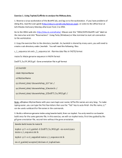

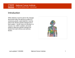


© Copyright 2026