High-Dimensional OLAP: A Minimal Cubing Approach∗
Xiaolei Li
Jiawei Han
Hector Gonzalez
University of Illinois at Urbana-Champaign, Urbana, IL 61801, USA
Abstract
Data cube has been playing an essential role
in fast OLAP (online analytical processing)
in many multi-dimensional data warehouses.
However, there exist data sets in applications
like bioinformatics, statistics, and text processing that are characterized by high dimensionality, e.g., over 100 dimensions, and moderate size, e.g., around 106 tuples. No feasible
data cube can be constructed with such data
sets. In this paper we will address the problem
of developing an efficient algorithm to perform
OLAP on such data sets.
Experience tells us that although data analysis tasks may involve a high dimensional space,
most OLAP operations are performed only
on a small number of dimensions at a time.
Based on this observation, we propose a novel
method that computes a thin layer of the
data cube together with associated value-list
indices. This layer, while being manageable
in size, will be capable of supporting flexible and fast OLAP operations in the original
high dimensional space. Through experiments
we will show that the method has I/O costs
that scale nicely with dimensionality. Furthermore, the costs are comparable to that of accessing an existing data cube when full materialization is possible.
1
Introduction
Since the advent of data warehousing and online analytical processing (OLAP) [9], data cube has been
∗ The work was supported in part by NSF IIS-02-09199.
Any opinions, findings, and conclusions or recommendations expressed in this paper are those of the authors and do not necessarily reflect the views of the funding agencies.
Permission to copy without fee all or part of this material is
granted provided that the copies are not made or distributed for
direct commercial advantage, the VLDB copyright notice and
the title of the publication and its date appear, and notice is
given that copying is by permission of the Very Large Data Base
Endowment. To copy otherwise, or to republish, requires a fee
and/or special permission from the Endowment.
Proceedings of the 30th VLDB Conference,
Toronto, Canada, 2004
playing an essential role in the implementation of fast
OLAP operations [10]. Materialization of a data cube
is a way to precompute and store multi-dimensional
aggregates so that multi-dimensional analysis can be
performed on the fly. For this task, there have
been many efficient cube computation algorithms proposed, such as ROLAP-based multi-dimensional aggregate computation [1], multiway array aggregation
[24], BUC [7], H-cubing [11], and Star-cubing [22].
Since computing the whole data cube not only requires
a substantial amount of time but also generates a huge
number of cube cells, there have also been many studies on partial materialization of data cubes [12], iceberg cube computation [7, 11, 22], computation of condensed, dwarf, or quotient cubes [19, 18, 13, 14], and
computation of approximate cubes [16, 5].
Besides large data warehouse applications, there are
other kinds of applications like bioinformatics, surveybased statistical analysis, and text processing that
need the OLAP-styled data analysis. However, data
in such applications usually are high in dimensionality, e.g., over 100 or even 1000 dimensions but only
medium in size, e.g., around 106 tuples. This kind of
datasets behaves rather differently from the datasets
in a traditional data warehouse which may have about
10 dimensions but more than 109 tuples. Since a data
cube grows exponentially with the number of dimensions, it is too costly in both computation time and
storage space to materialize a full high-dimensional
data cube. For example, a data cube of 100 dimensions, each with 10 distinct values, may contain as
many as 11100 aggregate cells. Although the adoption
of iceberg cube, condensed cube, or approximate cube
delays the explosion, it does not solve the fundamental
problem.
In this paper, we propose a new method called shellfragment. It vertically partitions a high dimensional
dataset into a set of disjoint low dimensional datasets
called fragments. For each fragment, we compute its
local data cube. Furthermore, we register the set of
tuple-ids that contribute to the non-empty cells in the
fragment data cube. These tuple-ids are used to bridge
the gap between various fragments and re-construct
the corresponding cuboids upon request. These shell
fragments are pre-computed offline and are used to
compute queries in an online fashion. In other words,
data cubes in the original high dimensional space are
dynamically assembled together via the fragments.
We will show that this method achieves high scalability in high dimensional space both in terms of storage space and I/O. When full materialization of the
data cube is impossible, our method provides a reasonable solution. In addition, as our experiments show,
the I/O costs of our method are competitive with those
of the materialized data cube.
The remainder of the paper is organized as follows.
In Section 2, we present the motivation of the paper. In Section 3, we introduce the shell fragment
data structure and design. In Section 4, we describe
how to compute OLAP queries using the fragments.
Our performance study on scalability, I/O, and other
cost metrics is presented in Section 5. We discuss the
related work and the possible extensions in Section 6,
and conclude our study in Section 7.
2
Analysis
Numerous studies have been conducted on data cubes
to promote fast OLAP. However, most cubing algorithms have been confined to only low or medium dimensional data. We shall show the inherent “curse of
dimensionality” of data cube in this section and provide motivation for our online computation model.
2.1
Curse of Dimensionality
The computation of data cubes, though valuable for
low-dimensional databases, may not be so beneficial for high-dimensional ones. Typically, a highdimensional data cube requires massive memory and
disk space, and the current algorithms are unable to
materialize the full cube under such conditions. Let’s
examine an example.
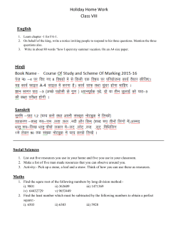
1600
Full Data Cube
Iceberg Cube, Minsup=5
Quotient Cube
1400
Cube Size (MB)
1200
1000
800
600
400
200
0
7
8
9
10
Dimensionality
11
12
Figure 1: The curse of dimensionality on data cubes
Example 1. We generated a base database of 600,000
tuples. Each dimension had a cardinality of 100 with
zipf equal to 2. The number of dimensions varies from
7 to 12 on the x-axis in Figure 1. The size of the
data cube generated from this base cuboid grows exponentially with the number of dimensions as shown
in Figure 1. The size of the full data cube reaches gigabytes when the number of dimensions reaches 9. And
it climbs to well above petabytes before it reaches 20
dimensions, not to think about 100 dimensions.
Figure 1 also shows the size of an iceberg cube with
minimum support of 5 for our database. It is much
smaller than the full data cube because the base cuboid
contains not many tuples and most high-dimensional
cells fall below the support threshold. This sounds attractive because it may substantially reduce the computation time and disk usage while keeping only the
“meaningful” results. However, there are several weaknesses. First, if a high-dimensional cell has the support already passing the iceberg threshold, it cannot
be pruned by the iceberg condition and will still generate a huge number of cells. For example, a basecuboid cell: “(a1 , a2 , . . . , a60 ):5” (i.e., with count 5)
will still generate 260 iceberg cube cells. Second, it is
difficult to set up an appropriate iceberg threshold. A
too low threshold will still generate a huge cube, but a
too high one may invalidate many useful applications.
Third, an iceberg cube cannot be incrementally updated. Once an aggregate cell falls below the iceberg
threshold and is pruned, incremental update will not
be able to recover the original measure.
The situation is not much better for condensed,
dwarf, or quotient cubes [19, 18, 13, 14]. The Dwarf
cube introduced in [18] compresses the cuboid cells by
exploiting sharing of prefixes and suffixes. Its size complexity was shown to be O(T 1+1/(logd C) ) [17] where d
is the number of dimensions, C is cardinality, and T is
the number of tuples. In high dimensional data where
d is large, logd C could become quite small. In which
case, the exponent becomes quite large and the cube
size still explodes.
For quotient cubes [13, 14], compression can only
be effective when the corresponding measures are the
same within a local lattice structure, which has limited
pruning power as shown in Figure 1.
Lastly, there is a substantial I/O overhead for accessing a full materialized data cube. Cuboids are
stored on disk in some fixed order, and that order
might be incompatible with a particular query. Processing such queries may need a scan of the entire corresponding cuboid.
One could avoid reading the entire cuboid if there
were multi-dimensional indices constructed on all
cuboids. But in a high-dimensional database with
many cuboids, it might not be practical to build all
these indices. Furthermore, reading via an index implies random access for each row in the cuboid, which
could turn out to be more expensive than a sequential
scan of the raw data.
A partial solution, which has been implemented in
some commercial data warehouse systems is to com-
pute a thin cube shell. For example, one might compute all cuboids with 3 dimensions or less in a 60dimensional data cube. There are two disadvantages
to
approach.
First, it still needs to compute
¢
¡60¢this ¡60
+
60
=
36050 cuboids. Second, it does
+
2
3
not support OLAP in a large portion of the highdimensional cube space because (1) it does not support OLAP on 4 or more dimensions (the shell only
offers shallow penetration of the entire data cube), and
(2) it cannot support drilling along even three dimensions, such as (A4 , A5 , A6 ), on a subset of data selected based on the constants provided in three other
dimensions, such as (A1 , A2 , A3 ). These types of operations require the computation of the corresponding
6-D cuboid, which the shell does not compute. In contrast, our model supports OLAP operations on the
entire cube space.
2.2
Computation Model
These observations lead us to consider possibly an online computation model of data cubes. It is quite expensive to online scan a high-dimensional database,
extract the relevant dimensions, and then perform onthe-spot aggregation. Instead, a semi-online computation model with certain pre-processing seems to be a
more viable solution.
Before delving deeper into the semi-online computation model, we make the following observation about
OLAP in high-dimensional space. Although a data
cube may contain many dimensions, most OLAP operations are performed only on a small number of dimensions at a time. In other words, an OLAP query is
likely to ignore many dimensions (i.e., treating them
as irrelevant), fix some dimensions (e.g., using query
constants as instantiations), and leave only a few to
be manipulated (for drilling, pivoting, etc.). This is
because it is not realistic for anyone to comprehend
the changes of thousands of cells involving tens of dimensions simultaneously in a high-dimensional space
at the same time. Instead, it is more natural to first locate some cuboids by certain selections and then drill
along one or two dimensions to examine the changes
of a few related dimensions. Most analysts only need
to examine the space of a small number of dimensions
once they select them.
3
Precomputation of Shell Fragments
Stemming from the above motivation, we propose a
new approach, called shell fragment, and two new algorithms: one for computing shell fragment cubes,
and one for query processing with the fragment cubes.
This new approach will be able to handle OLAP in
databases of extremely high dimensionality. It explores the inverted index well-studied in information
retrieval [4] and value-list index in databases [8]. The
general idea is to partition the dimensions into disjoint sets called fragments. The base dataset is pro-
jected onto each fragment, and data cubes are fully
materialized for each fragment. With the precomputed
shell fragment cubes, one can dynamically assemble
and compute cuboid cells of the original dataset online.
This is made efficient by set intersection operations on
the inverted indices.
3.1
Inverted Index
To illustrate the algorithm, a tiny database, Table 1,
is used as a running example. Let the cube measure
be count(). Other measures will be discussed later.
tid
1
2
3
4
5
A
a1
a1
a1
a2
a2
B
b1
b2
b2
b1
b1
C
c1
c1
c1
c1
c1
D
d1
d2
d1
d1
d1
E
e1
e1
e2
e2
e3
Table 1: The Original Database
The inverted index is constructed as follows. For
each attribute value in each dimension, we register a
list of tuple IDs (tids) associated with it. For example,
attribute value a2 appears in tuples 4 and 5. The tidlist for a2 then contains exactly 2 items, namely 4 and
5. The resultant inverted indices for the 5 individual
dimensions are shown in Table 2.
Attribute Value
a1
a2
b1
b2
c1
d1
d2
e1
e2
e3
TID List
123
45
145
23
12345
1345
2
12
34
5
List Size
3
2
3
2
5
4
1
2
2
1
Table 2: Inverted Indices for Individual Dimensions A,
B, C, D, and E
Lemma 1 The inverted index table uses the same
amount of storage space as the original database.
Rationale. Intuitively, we can think of Table 1 as storing the common TIDs for attributes and Table 2 as
storing the common attribute values for tuples. Formally, suppose we have a database of T tuples and
D dimensions. To store it as shown in Table 1 would
need D × T integers. Now consider the inverted index.
Each tuple ID is associated with D attributes and thus
will appear D times in the inverted index. Since we
have T tuple IDs in total, the entire inverted index
will still only need D × T integers1 .
3.2
Shell Fragments
The inverted index in Table 2 can be generalized to
multiple dimensions where one can store tid-lists for
combinations of attribute values across different dimensions. This leads to the computation of shell fragments of a data cube as follows.
All the dimensions of a data set are partitioned
into independent groups, called fragments. For each
fragment, we compute the complete local data cube
while retaining the inverted indices. For example, for
a database of 60 dimensions, A1 , A2 , . . . , A60 , we first
partition the 60 dimensions into 20 fragments of size
3: (A1 , A2 , A3 ), (A4 , A5 , A6 ), . . ., (A58 , A59 , A60 ). For
each fragment, we compute its full data cube while
recording the inverted indices. For example, in fragment (A1 , A2 , A3 ), we would compute seven cuboids:
A1 , A2 , A3 , A1 A2 , A2 A3 , A1 A3 , A1 A2 A3 . An inverted
index is retained for each cell in the cuboids. The
sizing and grouping of the fragments are non-trivial
decisions and will be discussed later in Section 4.3.
The benefit of this model can be seen by a simple
calculation. For a base cuboid of 60 dimensions, there
are only 7 × 20 = 140 cuboids to be computed according to the above shell fragment partition. Comparing
this to 36050 cuboids for the cube shell of size 3, the
saving is enormous.
Let’s return to our running example.
Example 2. Suppose we are to compute the shell
fragments of size 3. We first divide the 5 dimensions
into 2 fragments, namely (A, B, C) and (D, E). For
each fragment, we compute the complete data cube
by intersecting the tid-lists in Table 2 in a bottom-up
depths-first order in the cuboid lattice (as seen in [7]).
For example, to compute the cell {a1 b2 * }, we intersect the tuple ID lists of a1 and b2 to get a new list
of {2, 3}. Cuboid AB is shown in Table 3.
Cell
a1 b1
a1 b2
a2 b1
a2 b2
Intersection
123∩145
123∩23
45∩145
45∩23
Tuple ID List
1
23
45
∅
List Size
1
2
2
0
Table 3: Cuboid AB
After computing cuboid AB, we can then compute
cuboid ABC by intersecting all pairwise combinations
between Table 3 and the row c1 in Table 2. Notice
that because the entry a2 b2 is empty, it can be effectively discarded in subsequent computations based
on the Apriori property [2]. The same process can be
1 We assume that a TID and a value take the same unit space
(e.g., 4 bytes). Otherwise, the total space usage will differ proportionally to their unit space difference.
applied to computing fragment (D, E), which is completely independent from computing (A, B, C). Cuboid
DE is shown in Table 4.
Cell
d1 e1
d1 e2
d1 e3
d2 e1
Intersection
1345∩12
1345∩34
1345∩5
2∩12
Tuple ID List
1
34
5
2
List Size
1
2
1
1
Table 4: Cuboid DE
The computed shell fragment cubes with their inverted indices will be used to facilitate online query
computation. The question is how much space is
needed to store them. In our analysis, we assume an
array-like data structure to store the TIDs. If the cardinalities of the dimensions are small, bitmaps can be
employed to save space and speed up operations. This
and other techniques will be discussed in Section 6.
Lemma 2 Given a database of T tuples and D dimensions, the amount of memory needed to store the
F
shell fragments of size F is O(T ( D
F )(2 − 1)).
Rationale. Consider how many times each tuple ID will
be stored in the shell fragments. In the 1-dimensional
cuboids of the shell fragments, ¡Lemma
1 tells us each
¢
F
tuple ID will appear D = D
times.
Now conF 1
sider the 2-dimensional cuboids. Each tuple ID is associated with D dimensions and thus will be stored
anytime a cuboid is a¡ subset
of these D dimensions.
¢
F
There are exactly d D
F e 2 such 2-dimensional cuboids.
Sum over all cuboids (sizes 1 to F), we see
that the
P F ³ D ¡ F ¢´
entire shell fragment will need O(T i=1 d F e i )
F
= O(T ( D
F )(2 − 1)) storage space.
Based on Lemma 2, for our 60-dimensional base
cuboid of T tuples, the amount of space needed to
store the shell fragment of size 3 is on the order of
3
6
T ( 60
3 )(2 − 1) = 140T . Suppose there are 10 tuples
in the database and each tuple ID takes 4 bytes. The
space needed to store the shell fragments of size 3 is
roughly estimated as 140 × 106 × 4 = 560 MB.
3.2.1
Computing Other Measures
For the cube with only the tuple-counting measure,
there is no need to reference the original database for
measure computation since the length of the tid-list is
equivalent to tuple-count. “But what about other measures, such as average()?” The solution is to keep
an ID measure array instead of the original database.
For example, to compute average(), one just needs
to keep an array of three elements: (tid, count, sum).
The measures of every aggregate cell can be computed
by accessing this ID measure array only. Considering
a database with 106 tuples, each taking 4 bytes for tid
and 8 bytes for two measures, the ID measure array
is only 12 MB, whereas the corresponding database of
60 dimensions is (60 + 3) × 4 × 106 = 252 MB. To illustrate the design of the ID measure array, let’s look
at the following example.
Example 3. Suppose Table 5 shows an example
database where each tuple has 2 associated values,
count and sum.
tid
1
2
3
4
5
A
a1
a1
a1
a2
a2
B
b1
b2
b2
b1
b1
C
c1
c1
c1
c1
c1
D
d1
d2
d1
d1
d1
E
e1
e1
e2
e2
e3
count
5
3
8
5
2
sum
70
10
20
40
30
Algorithm 1 (Frag-Shells) Computation of shell
fragments on a given high-dimensional base table (i.e.,
base cuboid).
Input:
A base cuboid B of n dimensions:
(A1 , . . . , An ).
Output: (1) A set of fragment partitions {P1 , . . . Pk }
and their corresponding (local) fragment cubes
{S1 , . . . , Sk }, where Pi represents some set of dimension(s) and P1 ∪ . . . ∪ Pk are all the n dimensions, and
(2) an ID measure array if the measure is not tuplecount.
Method:
1.
Table 5: A database with two measure values
tid
1
2
3
4
5
count
5
3
8
5
2
sum
70
10
20
40
30
2.
3.
4.
5.
6.
7.
8.
Table 6: ID-measure array of Table 5
To compute a data cube for this database with the
measure avg() (obtained by sum()/count()), we need
to have a tid-list for each cell: {tid1 , . . . , tidn }. Because each tid is uniquely associated with a particular set of measure values, all future computations just
need to fetch the measure values associated with the
tuples in the list. In other words, by keeping an array
of the ID-measures in memory for online processing,
one can handle any complex measure computation.
Table 6 shows what exactly should be kept, which is
substantially smaller than the database itself.
Based on the above analysis, for a base cuboid of
60 dimensions with 106 tuples, our precomputed shell
fragments of size 3 will consist of 140 cuboids plus
one ID measure array, with the total estimated size of
roughly 560 + 12 = 572 MB in total. In comparison,
a shell cube of size 3 will consist of 36050 cuboids,
with estimated roughly 144 GB in size. A full 60dimensional cube will have 260 ≈ 1018 cuboids, with
the total cube size beyond the summation of the capacities of all storage devices. In this context, both
storage space and computation time of shell fragment
are negligible in comparison with those of the complete
data cube. Thus our high-dimensional OLAP on the
precomputed shell fragment can really be considered
as high-dimensional OLAP with minimal cubing.
3.2.2
Algorithm for Shell Fragment Computation
Based on the above discussion, the algorithm for shell
fragment computation can be summarized as follows.
partition the set of dimensions (A1 , . . . , An ) into
a set of k fragments P1 , . . . , Pk
scan base cuboid B once and do the following {
insert each htid, measurei into ID measure array
for each attribute value ai of each dimension Ai
build an inverted index entry: hai , tidlisti
}
for each fragment partition Pi
build a local fragment cube Si by
intersecting their corresponding tid-lists
and computing their measures
Note: For Line 1, Section 4.3 will discuss what kind
of partitions may achieve good performance. For Line
3, if the measure is tuple-count, there is no need to
build ID measure array since the length of the tid-list
is tuple-count; for other measures, such as avg(), the
needed components should be saved in the array, such
as sum() and count().
It is possible to use the above algorithm to compute
the full data cube: If we let a single fragment include
all the dimensions, the computed fragment cube is exactly the full data cube. The order of computation in
the cuboid lattice can be bottom-up and depth-first,
similar to that of [7]. This ordering also allows for
Apriori pruning in the case of iceberg cubes. We name
this algorithm Frag-Cubing.
4
Online Query Computation
Given the pre-computed shell fragments, one can perform OLAP queries on the original data space. In
general, there are two types of queries: (1) point query
and (2) subcube query.
A point query seeks a specific cuboid cell in the
original data space. All the relevant dimensions in
the query are instantiated with some particular values. In an n-dimensional data cube (A1 , A2 , . . . , An ),
a point query is in the form of ha1 , a2 , . . . , an : M i,
where each ai specifies a value for dimension Ai and
M is the inquired measure. For dimensions that are
irrelevant or aggregated, one can use * as its value.
For example, the query ha2, b1, c1, d1, ∗ : count()i
for the database in Table 1 is a point query where the
first four dimensions are instantiated to a2, b1, c1,
and d1 respectively, the last dimension is irrelevant,
and count() is the inquired measure.
A subcube query seeks a set of cuboid cells in the
original data space. It is one where at least one of
the relevant dimensions in the query is inquired. In
an n-dimensional data cube (A1 , A2 , . . . , An ), a subcube query is in the form of ha1 , a2 , . . . , an : M i,
where at least one ai is marked ? to denote that
dimension Ai is inquired. For example, the query
ha2, ?, c1, ∗, ? : count()i for the database in Table
1 is one where the first and third dimension values are
instantiated to a2 and c1 respectively, the fourth is
irrelevant, and the second and the fifth are inquired.
The subcube query computes all possible value combinations of the inquired dimension(s). It essentially
returns a local data cube consisting of the inquired
dimensions.
Conceptually, a point query can be seen as a special case of the subcube query where the number of
inquired dimensions is 0. On the other extreme, a
full-cube query is a subcube query where the number
of instantiated dimensions is 0.
4.1
Query Processing
The general query for an n-dimensional database is in
the form of ha1 , a2 , . . . , an : M i. Each ai has 3 possible values: (1) an instantiated value, (2) aggregate
*, (3) inquire ?. The first step is to gather all the instantiated ai ’s if there are any. We examine the shell
fragment partitions to check which ai ’s are in the same
fragments. Once that is done, we retrieve the tid-lists
associated with the instantiations at the highest possible aggregate level. For example, suppose aj and
ak were in the same fragment, we would then retrieve
the tid-list from the (aj , ak ) cuboid cell. The obtained
tid-lists are intersected to derive the instantiated base
table. If the table is empty, query processing stops and
returns the empty result.
If there are no inquired dimensions, we simply fetch
the corresponding measures from the ID measure array and finish the point query. If there is at least
one inquired dimension, we continue as follows. For
each inquired dimension, we retrieve all its possible
values and their associated tid-lists. If two or more
inquired dimensions are in the same fragment, we retrieve all their pre-computed combinations and the
tid-lists. Once these tid-lists are retrieved, they are
intersected with the instantiated base table to form
the local base cuboid of the inquired and instantiated
dimensions. Then, any cubing algorithm can be employed to compute the local data cube.
Example 4. Suppose a user wants to compute the
subcube query, {a2, b1, ?, *, ?: count()}, for
our database in Table 1. The shell fragments are precomputed as described in Section 3.2. We first fetch
the tid-list of the instantiated dimensions by looking at cell (a2, b1) of cuboid AB. This returns (a2,
b1):{4, 5}. Note that if there were no inquired dimensions in the query, we would finish the query here
and report 2 as the final count.
Next, we fetch the tid-lists of the inquired dimensions: C and E. These are {(c1:{1, 2, 3, 4, 5})}
and {(e1:{1, 2}), (e2:{3, 4}), (e3:{5})}. Intersect them with the instantiated base and we get
{(c1:{4, 5})} and {(e2:{4}), (e3:{5})}. This
corresponds to a base cuboid of two tuples: {(c1,
e2), (c1, e3)}. Any cubing algorithm can take this
as input and compute the 2-D data cube.
4.2
Algorithm for Shell
Query Processing
Fragment-Based
The above discussion leads to our algorithm for processing both point query and subcube query.
Algorithm 2 (Frag-Query) Processing of
and subcube queries using shell fragments.
point
Input: (1) A set of precomputed shell fragments for
partitions {P1 , . . . , Pk }, where Pi represents some
set of dimension(s), and P1 ∪ . . . ∪ Pk are all the
n dimensions; (2) an ID measure array if the measure is not tuple-count; and (3) a query of the form
ha1 , a2 , . . . , an : M i where each ai is either instantiated, aggregated, or inquired for dimension Ai . M is
the measure of the query.
Output: The computed measure(s) if the query is a
point query, i.e., containing only instantiated dimensions. Otherwise, the data cube whose dimensions are
the inquired dimensions.
Method:
1. for each Pi {
// instantiated dimensions
2.
if Pi ∩ {a1 , . . . , an } includes instantiation(s)
3.
Di ← Pi ∩ {a1 , . . . , an } with instantiation(s)
4.
BDi ← cells in Di with associated tid-lists
// inquired dimensions
5.
if Pi ∩ {a1 , . . . , an } includes inquire(s)
6.
Qi ← Pi ∩ {a1 , . . . , an } with inquire(s)
7.
RQi ← cells in Qi with associated tid-lists
}
8. if there exists at least one non-null BDi
9.
Bq ← merge base(BD1 , . . . , BDk )
10. if there exists at least one non-null RQi
11.
Cq ← compute cube(Bq , RQ1 , . . . , RQk )
Note: Function merge base() is implemented by intersecting the corresponding tid-lists of the BDi ’s. Function compute cube() takes the merged instantiated
base and the inquired dimensions as input, derive the
relevant base cuboid, and use the most efficient cubing algorithm to compute the multi-dimensional cube.
The ID measure array will be referenced after the cube
is derived in this compute cube() function.
4.3
Shell Fragment Grouping & Size
The decision of which dimensions to group into the
same fragments can be made based on the semantics
of the data or expectations of future OLAP queries.
The goal is to have many dimensions of a query fall
into the same fragments. This makes full use of the
pre-computed aggregates and saves both time and I/O.
In our examples, we chose equal-sized grouping of
consecutive dimensions in fragment partitioning. However, domain-specific knowledge can be used for better
grouping. For example, suppose in a 60-dimensional
data set, dimensions {A5 , A9 , A32 , A55 , A56 } often appear together in online queries, we can group them into
two fragments, such as (A5 , A9 , A32 ) and (A55 , A56 ), or
even one 5-D segment, depending on the historical or
expected frequent queries. Furthermore, the groupings need not to be disjoint. We could have two fragments, such as (A5 , A9 , A32 ) and (A9 , A55 , A56 ). This
added redundancy may offer speed-ups in query processing. With the known (or expected) query distribution and/or constraints on dimension set, intelligent
grouping can be performed to facilitate the retrieval
and manipulation of relevant set of dimensions within
a small number of fragments.
The decision of how many dimensions to group into
the same fragment can be analyzed more carefully.
Suppose each fragment contains an equal number of
dimensions and let that number be F. If F is too
small, the space required to store the fragment cubes
will be small but the time needed to compute queries
online will be long. On the other hand, if F is big,
online queries can be computed quickly but the space
needed to store the fragments will be enormous.
The question is whether there exists a F such that
there is a good balance between the amount of space
allocated to store the shell fragment cubes and the cost
(both time and I/O) of computing queries online.
First, we examine how space grows as a function
of F. Lemma 2 describes the exact function. It is
exponential with respect to F. However, notice that
when F is small, the growth is actually sub-linear. The
original database has size O(T D). When F = 2, the
memory usage is O(3/2T D), smaller than the linear
growth size of O(2T D). In fact, when F ≤ 4, the
growth in space is sub-linear.
Second, we examine the implications of F on query
performance. In general, a too small size, such as 1,
may lead to fetching and processing of rather long tid-
lists. Just having a F of 2 could greatly reduce this,
because many aggregates are pre-computed. Combine
this intuition with the previous paragraph, 2 ≤ F ≤ 4
seems like a reasonable range.
5
Performance Study
There are two major costs associated with our proposed method: (1) the cost of storing the shell fragment cubes, and (2) the cost of retrieving tid-lists and
computing the queries online. In this section, we perform a thorough analysis of these costs. All algorithms
were implemented using C++ and all the experiments
were conducted on an Intel Pentium-4 2.6CGHz system with 1GB of PC3200 RAM. The system ran Linux
with the 2.6.1 kernel and gcc 3.3.2.
As a notational convention, we use D to denote the
number of dimensions, C the cardinality of each dimension, T the number of tuples in the database, F
the size of the shell fragment, I the number of instantiated dimensions, Q the number of inquired dimensions, and S the skew or zipf of the data. Minimum
support level is 1 in all experiments.
5.1
Dimensionality and Storage Size
1000
50-C
100-C
750
Storage Size (MB)
Algorithm 2 covers all the possible OLAP queries.
In the case of point query, there exist no inquired dimensions, and Lines 6-7 and 11 are not executed. The
subcube query executes all the lines of the algorithm.
In the case of full-cube query, there are no instantiated dimensions, Lines 3-4 and 9 will not be executed.
Additionally, Bq is instantiated to all and the base
cuboid derived is essentially the original database.
500
250
0
20
30
40
50
60
Dimensionality
70
80
Figure 2: Storage size of shell fragments: (50-C) T =
106 , C = 50, S = 0, F = 3. (100-C) T = 106 , C =
100, S = 2, F = 2.
The first cost we are concerned with is the amount
of space needed to store the shell-fragment cubes.
Specifically, how it scales as dimensionality grows. Figure 2 shows the effect as dimensionality increases from
20 to 80. The number of tuples in both datasets were
106 . The first dataset, 50-C, has cardinality of 50, skew
of 0, and shell-fragment size 3. The second dataset,
100-C, has cardinality of 100, skew of 2, and shellfragment size 2. The good news is that storage space
grows linearly as dimensionality grows. This is expected because additional dimensions only add more
fragment cubes, which are independent of the others.
5.2
Shell-Fragment Size and Storage Size
1000
5.3
50-D
100-D
900
Storage Size (MB)
800
700
600
500
400
300
1
2
Shell Fragment Size
3
Figure 3: Storage size of shell fragments: (50-D) T =
106 , D = 50, C = 50, S = 0. (100-D) T = 106 , D =
100, C = 25, S = 2.
As discussed in Section 4.3, a fragment size between
2 and 4 strikes a good balance between storage space
and computation time. In this and the next couple of
subsections, we provide some test results to confirm
that intuition.
Figure 3 shows the storage size of the shell fragment cubes. Figure 4 shows the time needed to compute them. Our experiments were conducted on two
databases. The first, 50-D, has 106 tuples, 50 dimensions, cardinality of 50, and no skew. The second,
100-D, has 106 tuples, 100 dimensions, cardinality of
25, and zipf of 2. The shell-fragment size varies from
1 to 3.
Memory-Based Query Processing
As mentioned previously, the number of tuples in the
databases we are dealing with is in the order of 106
or less. In statistics studies, it is not unusual to find
datasets with thousands of dimensions but less than
one thousand tuples. Thus, it is reasonable to suggest that the shell fragment cubes could fit inside main
memory. Figure 3 shows with F equaling 3 or less, the
shell fragments for 50 and 100 dimensional databases
are under 1GB in size with 106 tuples.
In addition, recall our observation that many OLAP
operations in high dimensional spaces only revolve
around a few dimensions at a time. Most analysis will
pin down a small set of dimensions and explore combinations within the set. Through caching of the data
warehouse system, only the relevant dimensions and
their shell fragments need to reside in main memory.
With the shell fragments in memory, we can perform OLAP on the database with pure in-memory processes. Note that this would be impossible had we
chose to materialize the full data cube. Even with a
small tuple count, a data cube with 50 or more dimensions requires petabytes and cannot possibly be stored
in main memory.
In this section, we examine the implications of F
on the speed of in-memory query processing. In this
and the next subsection, we intentionally chose to have
small C values in order to make the subcube queries
meaningful. Otherwise in sparse uniform datasets, a
random instantiation often leads to an empty result.
60
Runtime (Milliseconds)
100
40
30
20
10
50
0
10
Point Query
2D Subcube Query
4D Subcube Query
50
50-D
100-D
150
Runtime (Seconds)
improved as F increases.
1
2
Shell Fragment Size
1
2
3
Shell Fragment Size
4
3
Figure 4: Time needed to compute shell fragments:
(50-D) T = 106 , D = 50, C = 50, S = 0. (100-D)
T = 106 , D = 100, C = 25, S = 2.
The sub-linear growth with respect to F ≤ 3 as
mentioned in Section 4.3 is confirmed here, both in
space and time. This is good news because as we will
show in the next few sections, overall performance is
Figure 5: Average computation time per query over
1,000 trials. T = 106 , D = 10, C = 10, S = 0, I = 4.
Figure 5 shows the time needed to compute point
and subcube queries with the shell fragments in memory. The Frag-Cubing algorithm is used to compute
the online data cubes. The database had 106 tuples,
10 dimensions of cardinality 10 each, and 0 zipf. Each
query had 4 randomly chosen instantiated dimensions,
and 0 (or 2 or 4) inquired dimensions. Other dimensions are irrelevant. The times shown are averages of
Point Query
2D Subcube Query
4D Subcube Query
Runtime (Milliseconds)
50
40
30
20
10
0
1
2
3
4
Shell Fragment Size
Figure 6: Average computation time per query over
1,000 trials. T = 106 , D = 20, C = 10, S = 1, I = 3.
1,000 such random queries. The 2D subcube queries
returned a table with 84 rows on average, and the 4D
subcube queries returned a table with 901 rows on average.
Figure 6 shows a similar experiment on another
database. The difference is that this database had
20 dimensions and each query had 3 randomly chosen
instantiated dimensions. The 2D subcube queries returned a table with 104 rows on average, and the 4D
subcube queries returned a table with 2,593 rows on
average.
The results show fast response time, with 50ms or
less for various types of queries. They show that having F ≥ 2 results in a non-trivial speed-up during
query processing over F = 1. If any of the instantiated dimensions are in the same fragment(s), the processing of the tid-lists is much quicker due to their
shorter lengths. If the inquired dimensions are in the
same fragment(s), the effects are less obvious because
the lengths of the tid-lists remain the same. The only
difference is that they have been pre-intersected.
The speed-up of F ≥ 2 is slightly less in Figure 6
than in Figure 5, partly because there are more dimensions overall. As a result, it is less likely for the
instantiated dimensions to be in the same fragment.
In real world datasets where there are semantics attached to the data, the fragments will be presumably
constructed so that they might be better matched to
the queries.
5.4
Disk-Based Query Processing
I/O with respect to shell-fragment size: In the
case that the shell fragments do not fit inside main
memory, the individual tid-lists relevant to the query
will have to be fetched from disk. In this section, we
study the effects of F on these I/O costs. With a
bigger F, more relevant dimensions in a query are
likely to be in the same fragment. This results in
retrieval of shorter tid-lists from disk because the
multi-dimensional aggregates are already computed
and stored.
Using the same two databases from the previous
subsection, we measured the average number of I/Os
needed to process a random query over 1,000 trials2 .
Figure 7 shows I/Os for computing point queries in the
10-D and 20-D databases. Figure 8 shows the same
for 4D subcube queries. No caching of tid-lists was
used between successive queries (i.e., cold-start in each
query testing).
In both graphs, I/O was reduced as F increased
from 1 to 4. This is because when instantiated dimensions were in the same fragments, their aggregated
tid-lists were much shorter for retrieval. In Figure 8,
the reduction was small relatively to the total I/O because there were 4 inquired dimensions. Since inquired
dimensions cover all tuples in the database, shell fragment sizes do not affect the I/O cost much.
400
I/O (Page Acceses)
60
10-D
20-D
300
200
100
1
2
3
4
Shell Fragment Size
Figure 7: Average I/Os per point query over 1,000
trials. (10-D) T = 106 , D = 10, C = 10, S = 0, I =
4, Q = 0; (20-D) T = 106 , D = 20, C = 10, S =
1, I = 3, Q = 0.
I/O cost: shell-fragments vs. full materialized
cubes: One may wonder how these I/O numbers compare to the case when full materialization of the data
cube is actually possible. In general, a query has I
instantiated dimensions and Q inquired dimensions.
In terms of the fully materialized cube, the query
seeks rows in the cuboid of all the relevant dimensions
(I + Q) with certain values according to the instantiations. For example, the query {?, ?, c1, *, e3, *}
seeks rows in the ABCE cuboid with certain values for
dimensions C and E. These rows are used to compute
all aggregates within dimensions A and B.
Because cuboid cells are stored on disk in some fixed
order, they might be incompatible with the query. For
example, they might happen to be sorted according to
the inquired dimensions first. In the worst case, the
entire cuboid of the relevant dimensions have to be retrieved. Further, it is necessary to read (I + Q + 1)
integers per row in the cuboid because we have to read
2 Assuming
4K page sizes and 4 bytes per integer.
10-D
20-D
Fragment-Based
Full Cube
6000
I/O (Page Accesses)
I/O (Page Acceses)
4300
4200
4100
5000
4000
3000
2000
1000
4000
1
2
3
4
Shell Fragment Size
Figure 8: Average I/Os per 4D subcube query over
1,000 trials. (10-D) T = 106 , D = 10, C = 10, S =
0, I = 4, Q = 4; (20-D) T = 106 , D = 20, C =
10, S = 1, I = 3, Q = 4.
the dimensional values and measure value. One may
argue that the dimensional values can be skipped if
there was an index on the cuboid cells. However, retrieval via an index implies random access for each row,
which turns out to be much more expensive than just
a plain sequential access with the dimensional values.
Figure 9 shows the average number of I/Os needed
in a random query of various sizes over 1,000 trials.
The number of inquired dimensions was 7 minus the
number of instantiated dimensions. No caching was
used, and the full data cube on disk was sorted according to the dimensional order: A, B, C, etc. Shell
fragment size was set to 1. The relevant dimensions
were the first 7 dimensions of the database and their
materialized cuboid contained 951,483 rows.
The curves show that the shell-fragment I/O is competitive with the materialized data cube in many cases.
Whenever the query had inquired dimensions before
the instantiated dimensions in terms of the sort order,
the materialized cuboid on disk have to pay the price
of scanning useless cells. On average, these costs turn
out be just as much as those in our method.
By having a shell-fragment size of 2 or more could
lower I/O costs for our method. In addition, in real
world applications with caching of recent queries, the
I/O costs for both methods would be drastically reduced. Furthermore, had there been fewer relevant
dimensions in the queries, the full data cube would
have achieved lower I/O numbers due to the smaller
cuboid size.
5.5
Experiments with Real-World Data Sets
Besides synthetic data, we also tested our algorithm on two real-world data sets. The first data
set was the Forest CoverType dataset obtained
from the UCI machine learning repository website
(www.ics.uci.edu/∼mlearn). This dataset contains
0
2
3
4
5
6
Number of Instantiated Dimensions
Figure 9: Average I/Os per query over 1,000 trials.
T = 106 , D = 10, C = 10, S = 0, F = 1, Q = 7 − I.
581,012 data points with 54 attributes, including 10
quantitative variables, 4 binary wilderness areas and
40 binary soil type variables. The cardinalities are
(1978, 361, 67, 551, 700, 5785, 207, 185, 255, 5827, 2,
2, 2, 2, 2, 2, 2, 2, 2, 2, 2, 2, 2, 2, 2, 2, 2, 2, 2, 2, 2, 2, 2,
2, 2, 2, 2, 2, 2, 2, 2, 2, 2, 2, 2, 2, 2, 2, 2, 2, 2, 2, 2, 2, 7).
We constructed shell-fragments of size 2 using consecutive dimensions as groupings. The construction took
33 seconds and 325MB.
With the shell fragments in memory, running a
point query with 1-8 instantiated dimensions took less
than 10 milliseconds. This is not surprising because
the number of tuples in the database is moderate.
More interesting are the subcube queries. Running
a 3-D subcube query with 1 instantiated dimension
ranged between 67 ms (millisecond) and 1.4 second.
Running a 5-D subcube query with 1 instantiated dimension ranged between 85 ms and 3.6 second. The
running times were extremely sensitive to the particular dimensions inquired in the query. The high-end
numbers reported were queries that included the dimension of cardinality 5827 in the inquired set. When
the cardinalities of the inquired dimensions are small,
subcube queries are extremely fast.
The second data set was obtained from the Longitudinal Study of the Vocational Rehabilitation Services
Program (www.ed.gov/policy/speced/leg/rehab/evalstudies.html). It has 8818 transactions with 24 dimensions. The cardinalities are (83, 9, 2, 7, 4, 3165, 470,
131, 1511, 409, 144, 53, 21, 14, 12, 13, 27, 21, 18, 140,
130, 50, 23, 505). We constructed shell-fragments of
size 3 using consecutive dimensions as the fragment
groupings. The construction took 0.9 seconds and
60MB.
With the shell fragments in memory, running a
point query on the dataset with 1-8 instantiated dimensions either in different fragments or the same took
basically no time. Running a 3-D subcube query with
no instantiations ranged between 50 ms and 1.6 sec-
ond. A 3-D subcube query with 1 instantiated dimension took on average only 90 ms to compute. A 5-D
subcube query with 0 instantiated dimensions ranged
between 227ms and 2.6 second. We also tried a similar
data set from the same collection with 6600 tuples and
96 dimensions and obtained very similar results.
6
Discussion
In this section, we discuss related work and further
implementation considerations.
6.1
Related Work
There are several threads of work related to our model.
First, partial materialization of data cubes has been
studied previously, such as [12]. Viewing the data
cube as a lattice of cuboids, some cuboids can be
computed from others. Thus to save storage space,
only the cuboids which are deemed most beneficial are
materialized and the rest are computed online when
needed. In this spirit, our approach may seem similar to theirs; however, the two models of computation
are very different. In our approach, low dimensional
cuboids facilitate the online construction of high dimensional cuboids via tid-lists. In [12], it is in the
opposite direction: high dimensional cuboids facilitate
the online construction of low dimensional cuboids by
further aggregation.
Our work utilizes the construct of an inverted index as termed in information retrieval and value-list
index as termed in databases. A large body of work
has been devoted to this area. Inverted index has been
widely used in information retrieval and Web-based information systems [4, 20]. Similar structures have been
proposed and used in bitmap index of data cubes [9]
and vertical format association mining [23]. Bitmaps
and other compression techniques have been studied to
optimize space and time usage [3, 8, 21]. In [15], projection indices and summary tables are used in OLAP
query evaluations. However, all of these works have
only focused on single dimensional indexing with or
without aggregation. Our model studies the construction of multi-dimensional data structures (i.e., 2-D, 3D fragments) and the corresponding measure aggregation. Such structures and pre-computations not only
reduce I/O costs but also speed up online computation
over the single dimensional counterparts.
In [6], the authors investigated the usage of low dimensional data structures for indexing a high dimensional space. Their method, tree-striping, also partitions a high dimensional space into a set of disjoint
low dimensional spaces. However, their data structures and algorithms were only designed to index data
points, lacking the aggregations and other elements
needed for data cubing.
One interesting observation made in [6] is that in
trying to optimize the tradeoffs between pre-calculated
result access and online computation, partitioning the
original space into sets of 2 or 3 dimensions was often
better than partitioning into single dimensions. Our
studies from the point of view of data cubing derives
a similar conclusion as they did for indexing: shellfragment sizes between 2 and 4 achieve a good balance
between storage size and online computation time.
6.2
6.2.1
Further Implementation Considerations
Incremental Update
The shell fragments and ID measure array are quite
adaptable to incremental updates. When a new tuple is inserted, a new htid : measurei pair is added
into the ID measure array. Moreover, this new tuple is vertically partitioned according to the existing
fragments and added to the corresponding inverted indices in the fragment cubes. Incremental deletion is
performed similarly with the reverse process. These
operations do not require the re-computation of existing data and are thus truly incremental. Furthermore,
query performance with incrementally changed data
is exactly the same as that of fragments re-computed
from scratch.
Another interesting observation is that one can
incrementally add new dimensions to the existing
data. This is difficult for normal data cubes. The
new dimensions (Di , . . . , Dj ) together with the new
data form new inverted lists, still in the form of
hdimension value : tidlisti. These new dimensions
can either form new fragments or be merged with the
existing ones. Similarly, existing dimensions can be
deleted by removing them from their respective fragments.
6.2.2
Bitmap Indexing
Throughout the paper, we have discussed I/O and
computation costs with the assumption that the tidlists are stored on disk as an array of integers. However, in data sets where cardinalities of the dimensions are small, bitmap indexing [3, 8, 15, 21] can improve space usage and speed. For example, if a column
only has 2 possible values: male or female, the savings
in storage space is high. Furthermore, the intersection operation can be performed much faster using the
bit-AND operation than the standard merge-intersect
operation.
6.2.3
Inverted Index Compression
Another compression method of the tid-lists come from
information retrieval [4, 20]. The main observation
is that the numbers in the tid-list are stored in ascending order. Thus, it would be possible to store a
list of d-gaps instead of the actual numbers. In general, for a list of numbers hd1 , d2 , . . . , dk i, the d-gap
list would be hd1 , d2 − d1 , . . . , dk − dk−1 i. For example, suppose we have the list h7, 10, 19, 22, 45i. The
d-gaps list would be h7, 3, 9, 3, 23i. The insight is that
the largest number in the d-gap list is bounded by the
difference between d1 and dk . Thus, it maybe possible
to store them using less than the standard 32 bits of
an integer. If many of the gap integers are small, the
compression could be substantial. The details of compression have been exploited in information retrieval.
Some of the popular techniques are unary, binary, δ,
γ, and Bernoulli [20].
7
Conclusions
We have proposed a novel approach for OLAP in highdimensional datasets with a moderate number of tuples. It partitions the high dimensional space into a
set of disjoint low dimensional spaces (i.e., shell fragments). Using inverted indices and pre-aggregated results, OLAP queries are computed online by dynamically constructing cuboids from the fragment data
cubes. With this design, for high-dimensional OLAPing, the total space that needs to store such shellfragments is negligible in comparison with a highdimensional cube, so is the online computation overhead. In our experiments, we showed that the storage cost grows linearly with the number dimensions.
Moreover, the query I/O costs for large data sets are
reasonable and are comparable with reading answers
from a materialized data cube, when such a cube is
available. And we also showed evidence of how different shell fragment sizes can affect query processing.
We have been performing further refinements of the
proposed approach and exploring many potential applications. Traditional data warehouses have difficulties at supporting fast OLAP in high dimensional data
sets, including spatial, temporal, multimedia, and text
data. A systematic study of the applications of this
new approach to such data could be a promising direction for future research.
References
[1] S. Agarwal, R. Agrawal, P. M. Deshpande, A.
Gupta, J. F. Naughton, R. Ramakrishnan and S.
Sarawagi. On the computation of multidimensional aggregates. In VLDB’96.
[2] R. Agrawal and R. Srikant. Fast algorithms for
mining association rules. In VLDB’94.
[3] S. Amer-Yahia and T. Johnson. Optimizing
queries on compressed bitmaps. In VLDB’00.
[4] R. Baeza-Yates and B. Ribeiro-Neto. Modern Information Retrieval. Addison-Wesley, 1999.
[5] D. Barbara and M. Sullivan.
Quasi-cubes:
Exploiting approximation in multidimensional
databases. SIGMOD Record, 26:12–17, 1997.
[6] S. Berchtold, C. B¨ohm, D. A. Keim, Hans-Peter
Kriegel, and Xiaowei Xu. Optimal multidimensional query processing using tree striping. In
DaWaK’00.
[7] K. Beyer and R. Ramakrishnan. Bottom-up computation of sparse and iceberg cubes. In SIGMOD’99.
[8] C. Y. Chan and Y. E. Ioannidis. Bitmap index
design and evaluation. In SIGMOD’98.
[9] S. Chaudhuri and U. Dayal. An overview of data
warehousing and OLAP technology. SIGMOD
Record, 26:65–74, 1997.
[10] J. Gray, S. Chaudhuri, A. Bosworth, A. Layman,
D. Reichart, M. Venkatrao, F. Pellow and H. Pirahesh. Data cube: A relational aggregation operator generalizing group-by, cross-tab and subtotals. Data Mining and Knowledge Discovery,
1:29–54, 1997.
[11] J. Han, J. Pei, G. Dong, and K. Wang. Efficient
computation of iceberg cubes with complex measures. In SIGMOD’01.
[12] V. Harinarayan, A. Rajaraman, and J. D. Ullman. Implementing data cubes efficiently. In SIGMOD’96.
[13] L. V. S. Lakshmanan, J. Pei, and J. Han. Quotient cube: How to summarize the semantics of a
data cube. In VLDB’02.
[14] L. V.S. Lakshmanan, J. Pei, and Y. Zhao. Qctrees: An efficient summary structure for semantic olap. In SIGMOD’03.
[15] P. O’Neil and D. Quass. Improved query performance with variant indexes. In SIGMOD’97.
[16] J. Shanmugasundaram, U. M. Fayyad, and P. S.
Bradley. Compressed data cubes for OLAP aggregate query approximation on continuous dimensions. In KDD’99.
[17] Y. Sismanis and N. Roussopoulos. The dwarf data
cube eliminates the high dimensionality curse.
TR-CS4552, University of Maryland, 2003.
[18] Y. Sismanis, N. Roussopoulos, A. Deligianannakis, and Y. Kotidis. Dwarf: Shrinking the
petacube. In SIGMOD’02.
[19] W. Wang, H. Lu, J. Feng, and J. X. Yu. Condensed cube: An effective approach to reducing
data cube size. In ICDE’02.
[20] I. H. Witten, A. Moffat, and T. C. Bell. Managing
Gigabytes: Compressing and Indexing Documents
and Images. Morgan Kaufmann, 1999.
[21] M. C. Wu and A. P. Buchmann. Encoded bitmap
indexing for data warehouses. In ICDE’98.
[22] D. Xin, J. Han, X. Li, and B. W. Wah. Starcubing: Computing iceberg cubes by top-down
and bottom-up integration. In VLDB’03.
[23] M. J. Zaki and C. J. Hsiao. CHARM: An efficient
algorithm for closed itemset mining. In SDM’02.
[24] Y. Zhao, P. M. Deshpande, and J. F. Naughton.
An array-based algorithm for simultaneous multidimensional aggregates. In SIGMOD’97.