
—A review Supersonic biplane Kazuhiro Kusunose , Kisa Matsushima
Progress in Aerospace Sciences 47 (2011) 53–87
Contents lists available at ScienceDirect
Progress in Aerospace Sciences
journal homepage: www.elsevier.com/locate/paerosci
Supersonic biplane—A review
Kazuhiro Kusunose a, Kisa Matsushima b,n, Daigo Maruyama c
a
b
c
JAXA, Japan
University of Toyama, Japan
ONERA, France
a r t i c l e i n f o
abstract
Available online 19 November 2010
One of the fundamental problems preventing commercial transport aircraft from supersonic flight is the
generation of strong sonic booms. Sonic booms are the ground-level manifestation of shock waves created by
airplanes flying at supersonic speeds. The strength of the shock waves generated by an aircraft flying at
supersonic speed is a direct function of both the aircraft’s weight and its occupying volume; it has been very
difficult to sufficiently reduce the shock waves generated by the heavier and larger conventional supersonic
transport (SST) configuration to meet acceptable at-ground sonic-boom levels. It is our dream to develop a
quiet SST aircraft that can carry more than 100 passengers while meeting acceptable at-ground sonic-boom
levels. We have started a supersonic-biplane project at Tohoku University since 2004. We meet the challenge
of quiet SST flight by extending the classic two-dimensional (2-D) Busemann biplane concept to a 3-D
supersonic-biplane wing that effectively reduces the shock waves generated by the aircraft. A lifted airfoil at
supersonic speeds, in general, generates shock waves (therefore, wave drag) through two fundamentally
different mechanisms. One is due to the airfoil’s lift, and the other is due to its thickness. Multi-airfoil
configurations can reduce wave drag by redistributing the system’s total lift among the individual airfoil
elements, knowing that wave drag of an airfoil element is proportional to the square of its lift. Likewise, the
wave drag due to airfoil thickness can also be nearly eliminated using the Busemann biplane concept, which
promotes favorable wave interactions between two neighboring airfoil elements. One of the main objectives
of our supersonic-biplane study is, with the help of modern computational fluid dynamics (CFD) tools, to find
biplane configurations that simultaneously exhibit both traits. We first re-analyzed using CFD tools, the classic
Busemann biplane configurations to understand its basic wave-cancellation concept. We then designed a 2-D
supersonic biplane that exhibits both wave-reduction and cancellation effects simultaneously, utilizing an
inverse-design method. The designed supersonic biplane not only showed the desired aerodynamic
characteristics at its design condition but also outperformed a zero-thickness flat-plate airfoil. (Zero-thickness
flat-plate airfoils are known as the most efficient monoplane airfoil at supersonic speeds.) Also discussed in
this paper is how to design 2-D biplanes, not only at their design Mach numbers but also at off-design
conditions. Supersonic biplanes have unacceptable characteristics at their off-design conditions such as flow
choking and its related hysteresis problems. Flow choking causes rapid increase of wave drag and it continues
to be kept up to the Mach numbers greater the cruise (design) Mach numbers due to its hysteresis. Some wing
devices such as slats and flaps, which could be used at take-off and landing conditions as high-lift devices,
were utilized to overcome these off-design problems. Then supersonic-biplane airfoils were extended to 3-D
wings. Because that rectangular-shaped 3-D biplane wings showed undesirable aerodynamic characteristics at
their wingtips, a tapered-wing planform was chosen for the study. A 3-D biplane wing having a taper ratio and
aspect ratio of 0.25 and 5.12, respectively, was designed utilizing the inverse-design method. Aerodynamic
characteristics of the designed biplane wing were further improved by using winglets at its wingtips. Flow
choking and its hysteresis problems, however, occurred at their off-design conditions. It was shown that these
off-design problems could also be resolved by utilizing slats and flaps. Finally, a study on the aerodynamic
characteristics of wing–body configurations was conducted using the tapered biplane wing. In this study a
body was chosen in order to generate strong shock waves at its nose region. Preliminary parametric studies on
the interference effects between the body and the tapered biplane wing were performed by choosing several
different wing locations on the body. From this study, it can be concluded that the aerodynamic characteristics
of the tapered biplane wing are minimally affected by the disturbances generated from the body, and that the
biplane wing shows promise for quiet commercial supersonic transport.
& 2010 Elsevier Ltd. All rights reserved.
n
Corresponding author. Tel./fax: + 81 76 445 6796.
E-mail addresses: [email protected], [email protected] (K. Matsushima).
0376-0421/$ - see front matter & 2010 Elsevier Ltd. All rights reserved.
doi:10.1016/j.paerosci.2010.09.003
54
K. Kusunose et al. / Progress in Aerospace Sciences 47 (2011) 53–87
Contents
1.
2.
3.
4.
5.
6.
7.
8.
Introduction . . . . . . . . . . . . . . . . . . . . . . . . . . . . . . . . . . . . . . . . . . . . . . . . . . . . . . . . . . . . . . . . . . . . . . . . . . . . . . . . . . . . . . . . . . . . . . . . . . . . . . . 54
History . . . . . . . . . . . . . . . . . . . . . . . . . . . . . . . . . . . . . . . . . . . . . . . . . . . . . . . . . . . . . . . . . . . . . . . . . . . . . . . . . . . . . . . . . . . . . . . . . . . . . . . . . . . 56
2.1.
Origin of the Busemann biplane . . . . . . . . . . . . . . . . . . . . . . . . . . . . . . . . . . . . . . . . . . . . . . . . . . . . . . . . . . . . . . . . . . . . . . . . . . . . . . . . . . 56
2.2.
Continuing research on the Busemann biplane . . . . . . . . . . . . . . . . . . . . . . . . . . . . . . . . . . . . . . . . . . . . . . . . . . . . . . . . . . . . . . . . . . . . . . 56
2.3.
Descendants and derivatives of the biplane concept . . . . . . . . . . . . . . . . . . . . . . . . . . . . . . . . . . . . . . . . . . . . . . . . . . . . . . . . . . . . . . . . . . 57
2-D theory and construction of biplane airfoils . . . . . . . . . . . . . . . . . . . . . . . . . . . . . . . . . . . . . . . . . . . . . . . . . . . . . . . . . . . . . . . . . . . . . . . . . . . 57
3.1.
Basic theory . . . . . . . . . . . . . . . . . . . . . . . . . . . . . . . . . . . . . . . . . . . . . . . . . . . . . . . . . . . . . . . . . . . . . . . . . . . . . . . . . . . . . . . . . . . . . . . . . . 57
3.1.1.
Wave-reduction effect . . . . . . . . . . . . . . . . . . . . . . . . . . . . . . . . . . . . . . . . . . . . . . . . . . . . . . . . . . . . . . . . . . . . . . . . . . . . . . . . . . 57
3.1.2.
Wave-cancellation effect (Busemann biplane) . . . . . . . . . . . . . . . . . . . . . . . . . . . . . . . . . . . . . . . . . . . . . . . . . . . . . . . . . . . . . . . 58
3.1.3.
An ideal biplane configuration, the Licher biplane . . . . . . . . . . . . . . . . . . . . . . . . . . . . . . . . . . . . . . . . . . . . . . . . . . . . . . . . . . . . 58
3.2.
CFD analysis . . . . . . . . . . . . . . . . . . . . . . . . . . . . . . . . . . . . . . . . . . . . . . . . . . . . . . . . . . . . . . . . . . . . . . . . . . . . . . . . . . . . . . . . . . . . . . . . . . 59
3.2.1.
Analyses using unstructured grid . . . . . . . . . . . . . . . . . . . . . . . . . . . . . . . . . . . . . . . . . . . . . . . . . . . . . . . . . . . . . . . . . . . . . . . . . 59
3.2.2.
Hysteresis analysis . . . . . . . . . . . . . . . . . . . . . . . . . . . . . . . . . . . . . . . . . . . . . . . . . . . . . . . . . . . . . . . . . . . . . . . . . . . . . . . . . . . . . 60
Design for biplane airfoil of better performance . . . . . . . . . . . . . . . . . . . . . . . . . . . . . . . . . . . . . . . . . . . . . . . . . . . . . . . . . . . . . . . . . . . . . . . . . . 63
4.1.
Inverse design . . . . . . . . . . . . . . . . . . . . . . . . . . . . . . . . . . . . . . . . . . . . . . . . . . . . . . . . . . . . . . . . . . . . . . . . . . . . . . . . . . . . . . . . . . . . . . . . 63
4.1.1.
Pressure and geometry relation . . . . . . . . . . . . . . . . . . . . . . . . . . . . . . . . . . . . . . . . . . . . . . . . . . . . . . . . . . . . . . . . . . . . . . . . . . 63
4.1.2.
Basic equation and procedure for the inverse-problem design . . . . . . . . . . . . . . . . . . . . . . . . . . . . . . . . . . . . . . . . . . . . . . . . . . 64
4.2.
Inverse design for biplane airfoil at a Mach number of 1.7 . . . . . . . . . . . . . . . . . . . . . . . . . . . . . . . . . . . . . . . . . . . . . . . . . . . . . . . . . . . . . 64
4.2.1.
Design process . . . . . . . . . . . . . . . . . . . . . . . . . . . . . . . . . . . . . . . . . . . . . . . . . . . . . . . . . . . . . . . . . . . . . . . . . . . . . . . . . . . . . . . . 64
4.2.2.
General features of the designed airfoil . . . . . . . . . . . . . . . . . . . . . . . . . . . . . . . . . . . . . . . . . . . . . . . . . . . . . . . . . . . . . . . . . . . . 65
4.3.
Drag polar diagrams . . . . . . . . . . . . . . . . . . . . . . . . . . . . . . . . . . . . . . . . . . . . . . . . . . . . . . . . . . . . . . . . . . . . . . . . . . . . . . . . . . . . . . . . . . . 67
3-D extension of biplane airfoils . . . . . . . . . . . . . . . . . . . . . . . . . . . . . . . . . . . . . . . . . . . . . . . . . . . . . . . . . . . . . . . . . . . . . . . . . . . . . . . . . . . . . . . 67
5.1.
Busemann biplane wing with rectangular planform . . . . . . . . . . . . . . . . . . . . . . . . . . . . . . . . . . . . . . . . . . . . . . . . . . . . . . . . . . . . . . . . . . 67
5.2.
Planform parametric study . . . . . . . . . . . . . . . . . . . . . . . . . . . . . . . . . . . . . . . . . . . . . . . . . . . . . . . . . . . . . . . . . . . . . . . . . . . . . . . . . . . . . . 68
5.2.1.
Effect of changing sweep angles . . . . . . . . . . . . . . . . . . . . . . . . . . . . . . . . . . . . . . . . . . . . . . . . . . . . . . . . . . . . . . . . . . . . . . . . . . 69
5.2.2.
Effect by changing taper ratios . . . . . . . . . . . . . . . . . . . . . . . . . . . . . . . . . . . . . . . . . . . . . . . . . . . . . . . . . . . . . . . . . . . . . . . . . . . 69
5.3.
Introduction of winglet . . . . . . . . . . . . . . . . . . . . . . . . . . . . . . . . . . . . . . . . . . . . . . . . . . . . . . . . . . . . . . . . . . . . . . . . . . . . . . . . . . . . . . . . . 69
5.4.
Design for better-performance biplane wing . . . . . . . . . . . . . . . . . . . . . . . . . . . . . . . . . . . . . . . . . . . . . . . . . . . . . . . . . . . . . . . . . . . . . . . . 70
5.4.1.
Application of the 2-D designed airfoil . . . . . . . . . . . . . . . . . . . . . . . . . . . . . . . . . . . . . . . . . . . . . . . . . . . . . . . . . . . . . . . . . . . . . 70
5.4.2.
3-D inverse design . . . . . . . . . . . . . . . . . . . . . . . . . . . . . . . . . . . . . . . . . . . . . . . . . . . . . . . . . . . . . . . . . . . . . . . . . . . . . . . . . . . . . 70
Wing–fuselage interference. . . . . . . . . . . . . . . . . . . . . . . . . . . . . . . . . . . . . . . . . . . . . . . . . . . . . . . . . . . . . . . . . . . . . . . . . . . . . . . . . . . . . . . . . . . 73
6.1.
Wing–fuselage configuration. . . . . . . . . . . . . . . . . . . . . . . . . . . . . . . . . . . . . . . . . . . . . . . . . . . . . . . . . . . . . . . . . . . . . . . . . . . . . . . . . . . . . 73
6.2.
Aerodynamic performance at cruise condition. . . . . . . . . . . . . . . . . . . . . . . . . . . . . . . . . . . . . . . . . . . . . . . . . . . . . . . . . . . . . . . . . . . . . . . 74
6.3.
Application of designed wing to wing–fuselage combination . . . . . . . . . . . . . . . . . . . . . . . . . . . . . . . . . . . . . . . . . . . . . . . . . . . . . . . . . . . 77
Experiment. . . . . . . . . . . . . . . . . . . . . . . . . . . . . . . . . . . . . . . . . . . . . . . . . . . . . . . . . . . . . . . . . . . . . . . . . . . . . . . . . . . . . . . . . . . . . . . . . . . . . . . . 80
Conclusions . . . . . . . . . . . . . . . . . . . . . . . . . . . . . . . . . . . . . . . . . . . . . . . . . . . . . . . . . . . . . . . . . . . . . . . . . . . . . . . . . . . . . . . . . . . . . . . . . . . . . . . 82
Acknowledgments . . . . . . . . . . . . . . . . . . . . . . . . . . . . . . . . . . . . . . . . . . . . . . . . . . . . . . . . . . . . . . . . . . . . . . . . . . . . . . . . . . . . . . . . . . . . . . . . . . 83
A.1. Aerodynamic center . . . . . . . . . . . . . . . . . . . . . . . . . . . . . . . . . . . . . . . . . . . . . . . . . . . . . . . . . . . . . . . . . . . . . . . . . . . . . . . . . . . . . . . . 83
A.1.1. Biplane and diamond airfoils. . . . . . . . . . . . . . . . . . . . . . . . . . . . . . . . . . . . . . . . . . . . . . . . . . . . . . . . . . . . . . . . . . . . . . . . 83
A.1.2. Relation between an A.C. location and load distributions . . . . . . . . . . . . . . . . . . . . . . . . . . . . . . . . . . . . . . . . . . . . . . . . . 84
References . . . . . . . . . . . . . . . . . . . . . . . . . . . . . . . . . . . . . . . . . . . . . . . . . . . . . . . . . . . . . . . . . . . . . . . . . . . . . . . . . . . . . . . . . . . . . . . . . . . . . . . . 86
1. Introduction
Beginning with the first flight achieved by the Wright brothers in
1903, the past 100 years of aviation history have been full of
remarkable milestones. In 1947, the Bell X-1 experimental aircraft
broke the sound barrier, ushering in the era of supersonic flight. In
military aviation, airplane speed records have been continuously
broken and topped; one of NASA’s experimental aircraft recently flew
at Mach-10 speeds. Commercial aviation, however, has not enjoyed
as many advances in supersonic flight; Concorde (1969–2003) was
the first but also the last supersonic transport aircraft ever built.
Concorde’s supersonic flights were, unfortunately, terminated, due to
its poor fuel efficiency and unacceptable at-ground noise level.
A fundamental problem preventing commercial transport
aircraft from supersonic flight is the creation of strong shock
waves, whose effects are felt on the ground in the form of sonic
booms. Because the strength of the shock waves generated by an
aircraft flying at supersonic speed is a direct function of both the
aircraft’s weight and its occupying volume, it has been deemed
nearly impossible to sufficiently reduce the shock waves generated by the heavier and larger conventional commercial aircraft to
meet acceptable at-ground sonic-boom levels. In this paper, we
focus on supersonic biplanes proposed by a group at Tohoku
University [1–6]. They tried to extend the classic Busemann
biplane concept [7–10] to develop a practical supersonic-biplane
wing that will generate sufficient lift at supersonic flights without
increasing a severe wave-drag penalty.
In general, a lifted airfoil generates shock waves through two
fundamentally different mechanisms: one is due to its lift and the
other is due to its thickness. The wave drag due to lift cannot be
eliminated completely; it can only be reduced through multi-airfoil
configurations. Based on the 2-D supersonic thin-airfoil theory [8]
wave drag of an airfoil is proportional to the square of its lift. Multiairfoil configurations redistribute the system’s total lift among the
individual airfoil elements, reducing the lift of each of the individual
elements and, therefore, the total wave drag of the system. This will
be referred to as the ‘‘wave-reduction effect’’ in the rest of this paper
[6]. Likewise, wave drag due to airfoil thickness can also be nearly
eliminated using the Busemann biplane concept, which promotes
favorable wave interactions between the two neighboring airfoil
elements. By choosing their geometries and their relative locations
strategically, the waves generated by the two elements cancel each
other (the ‘‘wave-cancellation effect’’ [6]). However, it is important to
remember that skin friction of the biplane system will increase
because of the increased surface area. One of the main objectives of
our supersonic-biplane study is, with the help of modern CFD tools,
K. Kusunose et al. / Progress in Aerospace Sciences 47 (2011) 53–87
Nomenclature
Symbols
A
An
A1, Ai
A2, At
Ain
AR
b
c, C
cmid
cref
croot
ctip
c1, c2
Cd
Cdp
Cdf
Cdfric
Cdtotal
CD
Cl
CL
Cp
D
f, g
f(x)
F
FU, FL
G, h
h
l
L
l/d
L/D
cross sectional area
cross sectional area at the throat of nozzle
section area of inlet
section area of throat
cross sectional area at the inlet of nozzle
aspect ratio
semi-span length
chord length
position of the mid-chord at the wingtip of the threedimensional wing
reference chord length
chord at the wing root of the three-dimensional wing
chord at the wingtip of the three-dimensional wing
Busemann coefficients
wave-drag coefficient of airfoil (wing section)
pressure drag coefficient of the two-dimensional
airfoil in Navier–Stokes simulations
friction drag coefficient of the two-dimensional airfoil
in Navier–Stokes simulations
friction drag coefficient
total drag coefficient in Navier–Stokes simulations
drag coefficient
lift coefficient (wing section)
lift coefficient
pressure coefficient
wave drag
function
airfoil geometry
pressure force acting on airfoil
pressure forces acting on upper and lower elements of
biplane
gap between biplane elements
gap between two elements of the biplane
surface length defined along the airfoil surface
lift
lift-to-drag ratio of the two-dimensional airfoil (wing
section)
lift-to-drag ratio
to obtain 2-D and 3-D biplane configurations that simultaneously
exhibit both traits.
Kusunose and his group at Tohoku University in 2004 began
to study supersonic biplanes for the next generation supersonic
transport by utilizing CFD tools (Navier–Stokes codes, but mainly
in their inviscid Euler modes) [11–13]. In this paper we introduce
a brief history of the classic Busemann biplane and its related
researches, followed by a discussion on the fundamental theory of
supersonic biplane. In general, supersonic biplanes show superior
aerodynamic characteristics at their design Mach numbers.
However, they have poor performances at their off-design
conditions. Flow choking occurs at high subsonic speeds [9,14],
and continues to Mach numbers greater than the design
Mach number in the acceleration stage due to flow hysteresis
[14,15]. Since the internal flow of a biplane is identical to that
of an intake diffuser, the characteristics of choking and hysteresis
of supersonic biplanes can be analyzed based on such
characteristics of a supersonic diffuser under start and un-start
conditions [16].
M
Msw
Mt
MN
MN
P
P0, PN
DP
q
r, y, xm
R
Re
Ds
S
t
UN
w
wlt
x, y, z
x
y
z
X, Y, Z
xi
xw
z
a
b, b0
g
d
e
y
y
m
r
55
Mach number
swallowing Mach number
Mach number behind oblique shock wave
free-stream Mach number
inlet Mach number
static pressure
total and free-stream pressures
pressure jump due to local flow inclination
dynamic pressure
parameters of skewed cylindrical coordinate system
gas constant
Reynolds number
entropy production
wing reference area
airfoil thickness
free-stream velocity
span width of biplane
winglet (wingtip panel)
parameters of the Cartesian coordinate system
streamwise coordinate
span-wise coordinate
vertical coordinate
body coordinate system
incident point from the leading edge
the location of wing for wing–fuselage configurations
gap between biplane elements
angle of attack
shock-wave angle
ratio of specific heats
margin
wedge angle
df/dx-a
reflection angle
Mach angle
fluid density
Subscripts
i
t
N
inlet
throat
free-stream
We then proceed with an overview of important progress made
by Kusunose’s group on 2-D and 3-D supersonic biplanes. It will be
discussed how to design supersonic biplanes, not only at their
design Mach numbers but also at their off-design conditions. At their
design Mach numbers, 2-D and 3-D supersonic biplanes that exhibit
both wave-reduction and wave-cancellation effects simultaneously
are designed using an inverse-design method [3,6,17,18]. At offdesign conditions hinged slats and flaps are applied to avoid flow
choking and accompanying hysteresis problems [6,17–22]. These
slats and flaps can be used as high-lift devices at take-off and
landing conditions. Several studies on sonic-boom propagation
mechanisms through the atmosphere are given in Ref. [23,24].
Aerodynamic studies on wing planforms and wing–body configurations are also conducted using a tapered biplane wing [25–30].
Preliminary parametric studies on the interference effect between
the body and biplane wing are performed by choosing several
different wing locations on the body [31,32]. We finally make a brief
review on recent experimental investigations closely related to
current biplane developments [33–39].
56
K. Kusunose et al. / Progress in Aerospace Sciences 47 (2011) 53–87
2. History
HIGH-SPEED AERONAUTICS
2.1. Origin of the Busemann biplane
Today, one can learn about the Busemann biplane only in a
traditional textbook. For example, in Liepmann and Roshko [8], it is
introduced as one of the wave-drag reduction methods utilizing
interference between its two element wings. The interference is
simply explained in Fig. 1, which is extracted from Ref. [8]. The
first proposal of the supersonic-biplane concept was made by
Dr. Adolf Busemann at the Fifth Volta Congress in Rome in 1935.
Fig. 2 shows a picture of the congress where many famous
aerodynamicists, including A. Busemann himself, are identified
[40]. This 1935 Volta Congress is regarded as the threshold of
modern high-speed aerodynamics. The main topic was ‘‘High
Velocity in Aviation,’’ with the President being G.A. Crocco. Here,
Busemann presented a paper titled ‘‘Aerodynamic lift at supersonic
speed’’ [7] in which he mostly discussed the concept of the swept
wing. In the supplement of the conference proceedings, Busemann
indicated how to cancel wave drag to make a wing equal to a
flat plane by means of biplane configuration. The article was
Wave-cancellation
Pressure distribution
on inside surface
Fig. 3. Busemann biplane proposed in (Ref. [41]).
written in German. Its title is ‘‘Auftribe des Doppeldeckers
bei Uebershallgeschwindigkeit’’, which means ‘‘Investigation of
Biplanes in Supersonic flows’’. Later, in 1955 in Ref. [41], he
presented the figure of the 1935 biplane again, which is shown in
Fig. 3. He introduced it as the biplane of zero wave drag and noise
that he had demonstrated at the Volta Congress in 1935.
2.2. Continuing research on the Busemann biplane
Wave reflection
Busemann biplane
Figure 1 of Ref. [41] titled “Biplane of zero drag and noise”.
Busemann biplane
Off-design
Fig. 1. Simple description for mutual cancellation of waves on a biplane (Ref. [8]).
C.Wieselsberger
A. Busemann
G.A.Crocco
L.Prandtl
Fig. 2. The Fifth Volta Congress (Ref. [40]). By the courtesy of http://www.dglr.de/
literatur/publikationen/pfeilfluegel/Kapitel1.pdf
After the Fifth Volta Congress, several researchers were
dedicated to the study of a supersonic biplane. Until 1958, studies
on Busemann-type biplanes appeared in many papers. Almost all
of the studies were two dimensional because of the lack of
computational power and refined experimental strategy when
compared with the technology of the present day.
V.O. Walcher carried out a parametric study regarding the
leading and trailing edge (L.E. and T.E.) angles of each upper and
lower element of a biplane [42].
In 1944, M.J. Lighthill discussed the advantages and disadvantages of the Busemann biplane. As a disadvantage, he pointed out
that the biplane had a greater wing area than a monoplane, which
increased skin-friction drag, and that the passage between the
two elements might ‘‘choke’’ [43]. In the same year, wind-tunnel
experiments were conducted by A. Ferri in Italy [14]. These were
done for both non-lifting and lifting cases. Ferri measured
aerodynamic forces and took Schlieren photographs to observe
the viscous effect of the boundary layer and shock movement
phenomena. He observed undesirable ‘‘choke’’ and ‘‘hysteresis’’
occurrences, both of which will be discussed later in this paper. In
spite of the disadvantages, Ferri concluded that the biplane was
promising to obtain better efficiency than that of an isolated wing.
In a 1947 NACA paper published in the United States,
W.E. Moeckel performed a detailed parametric study on the
spacing of the gap and the L.E. and T.E. angles of the two elements
of the biplane for lifting cases. One of his results was to find that
unsymmetrical biplanes whose lower elements were thicker
than upper elements would have higher L/D than symmetrical
biplanes [44].
Based on Moeckel’s conclusion, R.M. Licher made an analysis to
design the optimal L/D unsymmetrical biplane with the given Cl as
a constraint by using the supersonic linear theory in 1955 [10].
This is an interesting paper, which would lead us to a practical
supersonic-biplane transport. This will also be discussed in the
next chapter. After the publication of Ref. [10], however, no
further publication could be found in the literature except for
Ref. [45]. It appears that something had discouraged researchers
from further studying the Busemann biplane.
K. Kusunose et al. / Progress in Aerospace Sciences 47 (2011) 53–87
given by
2.3. Descendants and derivatives of the biplane concept
Inspired by the Busemann biplane concept, a lot of research
was inspired to consider the configuration wherein shock waves
interact with other multiple elements to produce favorable wave
interaction and reduce wave drag. Recently, in 2004, such
research was summarized in Ref. [46]. The author of Ref. [46],
Dr. D.M. Bushnell of NASA Langley Research Center, called the
concept the ‘‘favorable shock-wave-interference approach’’ for
drag reduction. He concluded that the issues of the concept can be
increasingly addressed through the progress of ‘‘smart material’’
and ‘‘flow control’’ technologies. Some of the issues such as the
derivatives of the biplane concept can be found in Refs. [47–49].
3. 2-D theory and construction of biplane airfoils
3.1. Basic theory
3.1.1. Wave-reduction effect
In this section we demonstrate the wave-reduction effect of
2-D biplanes. We compare the wave drag of two different airfoils,
a single flat-plate airfoil and a parallel flat-plate biplane, at a
supersonic flow condition. The conditions are such that both
airfoils generate the same amount of lift (the ‘‘constant-lift
condition’’). Using the 2-D (inviscid) supersonic thin-airfoil theory
[8], the local pressure jump can be expressed as a function of the
(small) local flow inclination angle a, measured from the
oncoming flow direction, as sketched in Fig. 4
DP
P1
¼
gM12
pp1
ffia
¼ qffiffiffiffiffiffiffiffiffiffiffiffiffi
P1
M12 1
57
ð1Þ
where g and M1 represent the ratio of specific heats and the Mach
number of the oncoming flow, respectively. Symbols P and P1 are
the local and oncoming flow pressures.
It can be shown that the lift and wave drag of a single flat-plate
airfoil with a small angle of attack aS as sketched in Fig. 5 are
4aS
LS ¼ pffiffiffiffiffiffiffiffiffiffiffiffiffiffiffi q1 C
2 1
M1
ð2Þ
4a2S
q1 C
DS ¼ pffiffiffiffiffiffiffiffiffiffiffiffiffiffiffi
2 1
M1
ð3Þ
where the symbols qN and C represent the free-stream dynamic
pressure defined by
q1 2
1
gM1
r U2 ¼
P1
2 1 1
2
and the chord length of the flat-plate airfoil, respectively [6,8].
Next, we calculate lift and drag of a biplane airfoil. The biplane,
as shown in Fig. 6, is constructed of two parallel flat plates having
the same chord length as that of the single flat plate C at an angle
of attack ab. Assuming that the compression wave (or expansion
waves) generated from the leading edge (L.E.) of one element does
not interact with the neighboring element, lift and drag of the
biplane can be calculated in the same way as they were calculated
for the single flat-plate airfoil [6].
The lift and drag of the biplane airfoil can be calculated as
follows:
8ab
Lb ¼ pffiffiffiffiffiffiffiffiffiffiffiffiffiffiffi
q1 C
2 1
M1
ð4Þ
8a2b
q1 C
Db ¼ pffiffiffiffiffiffiffiffiffiffiffiffiffiffiffi
2 1
M1
ð5Þ
We then adjust the biplane’s angle of attack ab such that the
constant-lift condition is met. Equating the lift of the biplane with
the lift produced by the single flat-plate airfoil (Eqs. (2) and (4)),
the two incidence angles ab and aS have the following
relationship:
ab ¼
aS
ð6Þ
2
Under the constant-lift condition, the wave drag of the biplane
reduces to
!
a 2
4a2S
8
1
S
pffiffiffiffiffiffiffiffiffiffiffiffiffiffiffi
Db ¼ pffiffiffiffiffiffiffiffiffiffiffiffiffiffiffi
q1 C
q1 C ¼
ð7Þ
2 1 2
2 1
2
M1
M1
Compared with Eq. (3), it is clear that the wave drag of the biplane
reduces to 1/2 of the original single-plate airfoil under the
constant-lift condition [6].
Fig. 4. Pressure jump through a compression or an expansion wave.
Fig. 5. Single flat-plate airfoil with angle of attack aS.
Fig. 6. Biplane airfoil with angle of attack ab.
58
K. Kusunose et al. / Progress in Aerospace Sciences 47 (2011) 53–87
Similarly, it can be easily shown that the wave drag of an
n-plate system reduces to 1/n of the original single-plate airfoil
under a specified lift condition, as long as the compression wave
(or expansion waves) generated from the L.E. of each element of
the n-plate biplane system does not interact with the neighboring
elements. We should remember, however, that skin-friction drag
of the n-plate airfoil will increase to n-times that of the single flatplate airfoil because of the increased surface area. The increase in
skin-friction drag is an inevitable byproduct of our wave-drag
reduction process using multi-element airfoil systems.
The skin friction of a single flat-plate airfoil can be estimated
using the following incompressible turbulent boundary-layer
formula [50]:
Cdfric ¼ 2Cf
Fig. 8. Pressure distribution on Busemann biplane.
ð8Þ
where
Cf ¼
0:027
ðReÞ1=7
ð9Þ
In this paper lift and drag coefficients of both single-plate and
biplane airfoils are defined by Cl L/qNC, Cd D/qNC based on the
chord length of single-plate airfoil C. The symbol Re denotes the
Reynolds number based on the flat-plate chord length, C. For the
conversion from incompressible to compressible flows, a relationship between the skin-friction coefficient (for incompressible
flows) and Mach number plotted in Fig. 13.10 of Ref. [8] can
be used.
3.1.2. Wave-cancellation effect (Busemann biplane)
The biplane configuration can also significantly reduce wave
drag due to airfoil thickness. Within a supersonic thin-airfoil
approximation, Busemann [7] showed that the wave drag of a
zero-lifted diamond airfoil can be completely eliminated by
simply splitting the diamond airfoil into two elements and
positioning them in a way such that the waves generated by
those elements cancel each other [8,9], as sketched in Fig. 7. The
wedge angles of the diamond airfoil and the Busemann biplane
are 2e and e, respectively. Remember that pressures acting on the
front half and rear half of its inner surfaces, P1 and P2, respectively
(see Fig. 8), are identical. Total lift and wave drag acting on the
Busemann biplane are, therefore, both zero under the zero-lift
condition.
Within a supersonic thin-airfoil approximation, lift and drag
acting on the Busemann biplane are identical to those acting on a
flat-plate airfoil at a small angle of attack [6,9]. However, in the
actual case wave drag is always larger than that of the flat-plate
airfoil, because of the entropy produced due to the shock waves
existing between the biplane elements.
Generally, in supersonic speeds, wave drag due to airfoil
thickness is large relative to that due to its lift. Supersonic aircraft
are therefore severely limited in their wing thickness. If the
Fig. 7. Wave-cancellation effect of Busemann biplane.
Fig. 9. Diamond airfoil at zero angle of attack.
Fig. 10. Wave-drag components of a diamond airfoil.
wave-cancellation effect is used effectively, the strong restriction
currently imposed on the wing thickness of supersonic aircraft
may be relaxed considerably. Remember that lift and wave
drag of a diamond airfoil (see Fig. 9) with a small incidence
angle a can be expressed, using the same supersonic thin-airfoil
approximation, as ([8])
4a
LD ¼ pffiffiffiffiffiffiffiffiffiffiffiffiffiffiffi q1 C þ 2 1
M1
ð10Þ
"
2 #
4
t
2
DD ¼ pffiffiffiffiffiffiffiffiffiffiffiffiffiffiffi a þ
q1 C þ UUU
2 1
C
M1
ð11Þ
Symbol t/C represents the thickness–chord ratio of the diamond
airfoil. In Fig. 10 wave-drag components due to lift and due to
thickness are calculated for a lifted diamond airfoil for two
different airfoil thicknesses t/C¼0.5 and 0.10 at constant-lift
condition Cl ¼ 0.10 and flow condition MN ¼1.7. Skin-friction
coefficients are calculated using Eq. (8), which is based on a flatplate airfoil with chord length C, with the help of the Mach
number correction factor given in Ref. 8.
3.1.3. An ideal biplane configuration, the Licher biplane
The previously discussed wave-reduction model (flat-plate
biplane model shown in Fig. 6), however, cannot be combined to
Busemann’s wave-cancellation concept directly, because wave
interactions that are required for the Busemann biplane do
not occur. We, therefore, need to seek a biplane configuration
that has those two desirable characteristics simultaneously in
order to attain a significant wave-drag reduction. An unsymmetrical
K. Kusunose et al. / Progress in Aerospace Sciences 47 (2011) 53–87
biplane configuration discussed by R. Licher in 1955 [10]
(sketched in Fig. 11) exhibits both of the desirable
characteristics: the wave-reduction effect and the wavecancellation effect. By promoting favorable wave interactions
between the upper and lower elements, the wave drag due to
lift can be reduced to 2/3 of that of a single flat plate under
the identical lift condition. Additionally, the Busemann wavecancellation concept can be applied to the system to eliminate
wave drag due to airfoil thickness. Wave-reduction effect of the
Licher biplane is discussed next.
Utilizing the supersonic thin-airfoil theory [8], the Licher
biplane can be split into its lift component and thickness
components, as shown in Fig. 11. Analysis of wave drag due to
thickness for the Licher biplane is identical to that of the
Busemann biplane, and has therefore been discussed in the
previous section. We, therefore, focus on lift and wave drag due to
its lift component. The symbol a denotes the flow inclination
angle of the upper (flat-plate) element; it also denotes the flow
inclination angle of the lower surface of the lower element
(see Fig. 12). The wedge angle of the lower element (having a halfdiamond shape) has been also chosen to be a. This particular
shape and location of the lower element cause the compression
wave generated from the leading edge of the upper element and
the expansion waves generated from the throat of the lower
element to cancel each other. This can be shown through
arguments similar to the wave-interaction analysis of the
Busemann biplane. Finally, we can show that the pressure along
the entire upper surface of the lower element is uniform, and that
its value is identical to that of the free-stream. It is, therefore,
clear that the upper element of the system acts like single flatplate airfoil with the incidence angle of a, and pressure acting
on the lower surface of the lower element contributes to the
system as an additional aerodynamic force. Detailed discussions
are given in [6].
59
Lift acting on the Licher biplane system shown in Fig. 12 can be
calculated as
!
4a
2a
3
4a
pffiffiffiffiffiffiffiffiffiffiffiffiffiffiffiq1 C
L ¼ pffiffiffiffiffiffiffiffiffiffiffiffiffiffiffi q1 C þ pffiffiffiffiffiffiffiffiffiffiffiffiffiffiffi q1 C ¼
ð12Þ
2 1
2 1
2 1
2
M1
M1
M1
Comparing Eq. (12) with Eq. (2), it is clear that the Licher biplane
generates 1.5 times the lift of a single flat-plate airfoil with the
same angle of attack. We now adjust the angle of attack a of the
Licher biplane so that it generates the same amount of lift as a
single flat-plate airfoil with an angle of attack aS (constant-lift
condition). Since both the single and Licher airfoils have the same
reference chord length C, a and aS have the following relationship:
2
3
a ¼ aS
ð13Þ
Because of the constant-lift condition
!
3
4a
4aS
pffiffiffiffiffiffiffiffiffiffiffiffiffiffiffiq1 C ¼ pffiffiffiffiffiffiffiffiffiffiffiffiffiffiffi
q1 C ¼ LSingle
L¼
2 1
2 1
2
M1
M1
ð14Þ
Similar to the lift analysis, wave drag of the Licher biplane system
can be expressed as ([6])
!
4a2
2a2
3
4a2
pffiffiffiffiffiffiffiffiffiffiffiffiffiffiffiq1 C
D ¼ pffiffiffiffiffiffiffiffiffiffiffiffiffiffiffi q1 C þ pffiffiffiffiffiffiffiffiffiffiffiffiffiffiffi q1 C ¼
ð15Þ
2 1
2 1
2 1
2
M1
M1
M1
When the constant-lift condition (L¼LSingle) is considered, the
drag Eq. (15) reduces (with the help of Eq. (13)) to
!
!
2
4a2S
3
4
2
2
2
pffiffiffiffiffiffiffiffiffiffiffiffiffiffiffi
pffiffiffiffiffiffiffiffiffiffiffiffiffiffiffiq1 C ¼ DSingle
aS q1 C ¼
D¼
2 1 3
2 1
2
3
3
M1
M1
ð16Þ
Eq. (16) shows that the wave drag due to lift of the Licher
biplane reduces to 2/3 that of a single flat-plate airfoil under
constant-lift condition [6,10].
3.2. CFD analysis
Fig. 11. Decomposition of Licher Biplane into its lift and thickness components.
3.2.1. Analyses using unstructured grid
In this section, analysis results from CFD simulations using an
unstructured grid approach are mentioned [18–20]. For the
purpose of examining the characteristics of Busemann biplanes
at off-design conditions with zero incidence angle, the thickness–
chord ratio (t/c) of the Busemann biplane and a diamond airfoil
were selected as 0.10 (its equivalent wedge angle, e, being 5.711)
(shown in Fig. 13). The gap of the biplane has been adjusted
(z/c¼0.5) to obtain minimum drag at free-stream Mach number,
MN ¼1.7, which will be referred as the design Mach number
hereinafter in this paper. Inviscid flow analyses were performed
using the TAS code (Ref. [51,52]). The grids around the diamond
airfoil and the Busemann biplane are shown in Fig. 14. Wave-drag
coefficient (Cd) calculated from CFD analyses and theory based on
the supersonic thin-airfoil approximation are shown in Table 1.
They are in good agreement. The reliability of the CFD code was
Busemann biplane
Diamond airfoil
t1
z
t2
c
(z/c=0.5, t/c=0.10)
Fig. 12. Geometry of lift component of Licher Biplane.
t
c
t1=t2
(t/c=0.10)
Fig. 13. Baseline models at zero-lift conditions (MN ¼ 1.7).
60
K. Kusunose et al. / Progress in Aerospace Sciences 47 (2011) 53–87
Zero-Lift conditions
0.16
Busemann Biplane
Busemann
Biplane
Diamond Airfoil
Diamond
Airfoil
0.14
t z
0.12
c
Cd
0.10
(z/c=0.5, t/c=0.05)
t
0.08
c
(t/c=0. 10)
0.06
0.04
Fig. 14. Mesh visualizations of a Busemann biplane baseline model (twodimensional unstructured grid, grid numbers are 0.20 million).
0.02
0.00
0.0
0.5
1.0
1.5
2.0
2.5
3.0
M
Diamond airfoil
Busemann biplane
CFD
Theory
Error (%)
0.0291
0.00189
0.0292
–
0.34
–
discussed and validated in Ref. (6). It is clear that wave drag of the
Busemann biplane is almost completely eliminated being less
than 1/10 of that of the diamond airfoil.
Because the biplane configuration is similar to the supersonic
converging and diverging nozzle, supersonic biplanes may have
the disadvantage of having choked flow at a wide range of
transonic flow regions. The choked-flow phenomenon generates
significant wave drag at the biplane’s off-design Mach numbers.
Fig. 15 shows the detailed wave-drag characteristics of the
Busemann biplane over a range of flight Mach numbers
(0.3o MN o3.0), including its design Mach number MN ¼1.7.
Flow-hysteresis problem that caused by the continuous change in
the free-stream Mach number will not be considered. CFD
analyses, including the flow-hysteresis problem, will be
discussed in the next section. Flow choking and its concomitant
hysteresis problem were also observed in experiments [14,34,35].
Let us now return to Fig. 15 again. We can observe a range of
Mach numbers (1.64oMN o2.0) where wave drag remains
nearly at its minimum value. The existence of this low wavedrag range is critical for the development of actual airplanes in the
future. From Fig. 15, however, we also observe a high wave-drag
range of Mach numbers in the transonic flow region where wave
drag is even greater than that of the baseline diamond airfoil.
Some of the strategies to counter against choking (high drag)
are airfoil morphing and the adaptation of Fowler motion. Figs. 16
and 17 show simple diagrams of morphing and Fowler motion
used in this study. Morphing alters the area ratio of the inlet area
to the throat. With the morphing strategy, reduction in wave drag
is expected because of the change in airfoil thickness. The
thickness–chord ratio (t/c) is changed from 0.10 to 0.06 on each
element as shown in Fig. 16.
Fig. 18 shows wave-drag characteristics at various Mach
numbers of the Busemann biplane with morphing and with
Fowler motion. It can be observed that much lower wave drag
than that of the diamond airfoil is achieved over a wide range of
free-stream Mach numbers [6,18]. However, it is obvious that the
biplane with Fowler motion has higher friction drag than other
biplanes because of the increase in surface area.
3.2.2. Hysteresis analysis
In real flight, airplanes accelerate from take-off to cruise Mach
number continuously. During the acceleration stage, choking will
Fig. 15. Wave-drag characteristics of the diamond airfoil and the Busemann
biplane (zero lift).
Fig. 16. A simple diagram of the Busemann biplane with morphing.
Fig. 17. A simple diagram of the Busemann biplane with Fowler motion.
0.16
Busemann Biplane
Diamond Airfoil
Morphing
Fowler
0.14
0.12
0.10
Cd
Table 1
Wave-drag coefficients (Cd) of a diamond airfoil and a Busemann biplane
(zero lift).
0.08
0.06
0.04
0.02
0.00
0.0
0.5
1.0
1.5
M
2.0
2.5
3.0
Fig. 18. Wave-drag characteristics of the biplane with morphing (zero lift).
occur and it may cause flow-hysteresis problems. Therefore it is
necessary to simulate the actual processes by changing the
airplane speed continuously.
3.2.2.1. One-dimensional theory on intake diffuser. It is necessary to
discover methods that are applicable to Busemann-type biplanes
in order to avoid the choked-flow and flow-hysteresis problems at
off-design conditions. Before we examine how these problems can
be overcome, it may be useful to discuss the start/un-start characteristics of a supersonic inlets diffuser (see Fig. 19), for they
K. Kusunose et al. / Progress in Aerospace Sciences 47 (2011) 53–87
61
share many similar characteristics with the Busemann biplane. In
Fig. 19, the line in red shows the Kantrowitz limit [16,53] (given
by Eq. (17)), which is the Mach number that the flow speed of
inlet diffusers must exceed before the inlets can go from the unstart to start condition, once a bow shock is generated in front of
its inlet.
1=2 1=ðg1Þ
2
2
At
ðg1ÞM1
þ2
2gM1
ðg1Þ
¼
ð17Þ
2
2
Ai
ðg þ1ÞM1
ðg þ1ÞM1
It is reasonable to assume that this rule can be applied to the
Busemann biplane in order to avoid the choked-flow and flowhysteresis of the Busemann biplane. In fact, the results from CFD
analyses are in good agreement with the values that are
calculated using Eqs. (17) and (18). Here the At/Ai of the
Busemann biplane is 0.8, as shown by the solid line in Fig. 19.
The predicted Mach number of the starting and unstarting are
2.154 and 1.600, respectively.
where Ai is the area of inlet and At is the area of throat. Also, the
line in blue refers to the isentropic contraction limit [53], where
the Mach number is MN ¼1.0 at the throat of supersonic inlets.
The isentropic contraction limit is calculated by Eq. (18).
ðg þ 1Þ=2ðg1Þ
2
At
ðg1ÞM1
þ2
¼ M1
ð18Þ
Ai
gþ1
3.2.2.2. Quasi-unsteady CFD simulations. Inviscid CFD analyses
(Euler simulation) of the Busemann biplane were conducted to
trace the hysteresis. For the simulation we use the following
strategy: a quasi-unsteady simulation. We divide the acceleration
process from 0.6 to 2.18 of free-stream Mach numbers into small
intervals of 0.1 or so. We conducted a series of simulations as MN
was raised discretely along the intervals using the previous
simulation result imposed as the initial condition.
Figs. 20 and 21 show Cp color maps at each Mach number in
acceleration and deceleration stages. Fig. 22 shows a Cd–MN graph.
We observe that a detached shock wave is generated at an upstream
location of the airfoils and it gets closer to the leading edge with
each increment of a free-stream Mach number. Once a certain Mach
number is reached, the detached shock wave attaches to the leading
edge and is swallowed to a downstream location of the throat. As a
consequence, choking disappears (in this case at MN ¼2.18).
This phenomenon is similar to that of the starting process of the
intake diffuser. The value of the starting Mach number given
from CFD agrees with that predicted from the 1-D flow equation
(Eq. (17)).
Kantrowitz limit
Isentropic Contraction limit
Ai
At
Fig. 19. Start/un-start characteristics of supersonic inlet diffuser.
3.2.2.3. How to minimize hysteresis problem. From Fig. 19 it is
evident that as the area ratio At/Ai increases, the biplane becomes
more and more startable at lower Mach numbers. The biplane
equipped with hinged slats and flaps, shown in Fig. 23, was used
for the study. With the hinged slat the sectional area ratio of the
inlet to the throat (At/Ai) increases to 0.909. According to the
Fig. 20. Cp color maps around the Busemann biplane on acceleration (from 0.6 to 2.18 of free-stream Mach number per about 0.1) (0.6 r MN r1.1); (1.2r MN r1.7) and
(1.8r MN r 2.18). (For interpretation of the references to color in this figure legend, the reader is referred to the web version of this article).
62
K. Kusunose et al. / Progress in Aerospace Sciences 47 (2011) 53–87
Fig. 23. A simple diagram of the Busemann biplane equipped with hinged slats
and flaps.
Fig. 24. Cp color maps of the biplane equipped with hinged slats and flaps on
acceleration (zero lift). (For interpretation of the references to color in this figure
legend, the reader is referred to the web version of this article).
0.16
0.14
0.16
Impalsive start Analyses
0.14
Acceleration
Cd
0.06
0.00
0.0
0.08
M =1.64
1.0
1.5
M
2.0
2.5
M =2.18
M =1.56
1.0
1.5
M
2.0
2.5
Design Mach number
M =1.7
M =2.18
0.5
Hysteresis
0.02
0.08
0.02
Slat and Flap Acceleration
0.10
0.00
0.5
0.04
Acceleration
0.04
Hysteresis
0.10
Busemann
0.06
Deceleration
0.12
Deceleration
Slat and Flap Deceleration
0.12
Cd
Fig. 21. Cp color maps around the Busemann biplane on deceleration (from 2.18 to
1.7 of free-stream Mach number per about 0.1) (2.18 Z MN Z1.7). (For
interpretation of the references to color in this figure legend, the reader is referred
to the web version of this article).
Busemann
3.0
Fig. 25. Wave-drag characteristics of the Busemann biplane and the one equipped
with hinged slats and flaps on quasi-unsteady flow (zero lift).
Design Mach number
M =1.7
Fig. 22. Wave-drag characteristics of Busemann biplane on quasi-unsteady flow
(zero lift).
equations of the intake diffuser, the biplane equipped with hinged
slats and flaps can start at MN ¼1.55. Choking will no longer occur
at the cruise Mach number (MN ¼1.7).
CFD analyses were conducted on the Busemann biplane
equipped with slats and flaps using a quasi-unsteady simulation
[6,18,21]. Fig. 24 shows Cp color maps near the starting Mach
number. Fig. 25 shows a Cd–MN graph. We can see the starting
occurs at MN ¼1.56 and that choking disappears. Note that based
on the one-dimensional theory from Eq. (17), the predicted
starting Mach number is 1.55. For the Busemann biplane with
morphing discussed in the previous section (see Fig. 16), the
starting condition is MN ¼ 1.41. The ratio of the section area of the
inlet to that of the throat (At/Ai) is 0.936 (With the theoretical
starting Mach number being 1.40).
K. Kusunose et al. / Progress in Aerospace Sciences 47 (2011) 53–87
63
Cp
Eddy viscosity
Fig. 26. A simple diagram of the Busemann biplane equipped with hinged slats
and flaps utilized as a high-lift-device.
Busemann biplane
2.5
Cp
2
2
3
4
5
6
7
Eddy viscosity
8
1
0
1.5
Cl
-1
1
every 1degree plotted
5
0.5
3
2
Busemann
Busemann
biplane
biplane
with HLD
with
1
0
0
0
Busemann
Busemann
biplane
biplane
0.05
0.1
0.15
0.2
HLD
Busemann biplane equipped with slats (10deg) and flaps (15deg)
0.25
Cdtotal
Fig. 27. Drag polar diagram of the Busemann biplane and the one equipped with
hinged slats and flaps utilized as a high-lift-device angle of attack 41.
3.2.2.4. High-lift condition. In this section, take-off and landing
conditions (MN ¼0.2) are discussed [6,18]. The Navier–Stokes
equation was used for the analyses, with a Reynolds number of 30
million. A one-equation turbulence model by Spalart–Allmaras
[54] is adopted to treat turbulent boundary layers for viscous flow
computations. The same hinged slats and flaps mentioned before
are used as a high-lift-device. The geometry used for the analysis
is shown in Fig. 26. The positions of the hinges are the same as
those of the biplane shown in Fig. 23 (30% chord length). Fig. 27
shows a drag polar diagram (where, Cdtotal refers to the total drag
coefficient: wave drag plus friction drag) and Fig. 28 shows Cp and
eddy viscosity color maps at an angle of attack of 41. The
calculated lift and drag are given in Table 2. It can be observed
that sufficient lift (Cl 42.0) is generated by utilizing hinged slats
and flaps.
Viscous effects at off-design conditions are also discussed
briefly. Fig. 29 shows Cdtotal characteristics near its start and unstart Mach numbers. Here, results from both Navier–Stokes and
Euler simulations are compared. It shows that there are no drastic
changes in flow characteristics caused by viscous effects, with the
exception of the starting Mach (reduced from 2.18 to 2.14).
Fig. 28. Cp and eddy viscosity color maps of the Busemann biplane and the one
equipped with slats and flaps as a high-lift-device (A.o.A¼ 41). (For interpretation
of the references to color in this figure legend, the reader is referred to the web
version of this article).
Table 2
CFD analysis results of both two biplanes at an angle of attack 41.
Busemann biplane
HLD
4.1. Inverse design
4.1.1. Pressure and geometry relation
As discussed in the previous section, biplane airfoils can be
good candidates for the wings of next generation SST. We,
therefore employed inverse designing to optimize the biplane
airfoil at its lifted condition. The inverse-design process calculates
Cdtotal
0.612
2.025
0.0485
0.0955
Euler Acceleration
Euler Deceleration
NS Acceleration
NS Deceleration
0.10
0.08
0.06
M =2.14
0.04
M =2.18
0.02
0.00
1.2
4. Design for biplane airfoil of better performance
Cl
0.12
Cdtotal
4
M =1.64
2.2
1.7
Design Mach number
M =1.7
M
Fig. 29. Cd characteristics of the Busemann biplane on quasi-unsteady simulation
over a range of free-stream Mach numbers (Euler and Navier–Stokes analyses).
the airfoil geometry, necessary for the specified target pressure
distribution to occur along its surface [6,17–19]. In order to
determine the desired geometry, the relationship between the
64
K. Kusunose et al. / Progress in Aerospace Sciences 47 (2011) 53–87
surface pressure distribution and geometry is required. Here, we
use an algebraic relationship derived from the oblique shock
relations [8].
An airfoil’s geometry f(x) is related to its pressure distribution,
as follows:
Cp ¼ c1 y þ c2 y
2
ð19Þ
z
c2 ¼
ðM1 2 2Þ2 þ gM1 4
2ðM1 2 1Þ2
x
Fig. 31. Airfoil geometries based on the current and target pressure distributions.
Initial Airfoil
Target Cp
Cp
Grid Generation
ð20Þ
a is the angle of attack of the airfoil. Also, x represents the airfoilchord direction (see Fig. 30) and g is the ratio of specific heats. MN
( 41.0) is the free-stream Mach number.
Eq. (19) is the second-order equation with respect to change in
geometry. Splitting the airfoil geometry into the upper and lower
surfaces, Eq. (19) yields
2
df þ ðxÞ
df þ ðxÞ
Cp þ ¼ c 1
a þc2
a
dx
dx
2
df ðxÞ
df ðxÞ
Cp ¼ c1
ð21Þ
a þ c2
a
dx
dx
f(x)+ Δ f(x)
Flow
A.O.A = α
where y represents the local flow deflection angle (df/dx a) along
the airfoil surface. The symbols c1, c2, are the Busemann
coefficients given as
2
c1 ¼ qffiffiffiffiffiffiffiffiffiffiffiffiffiffiffiffiffi ,
M1 2 1
f (x)
Cp
Target Cp
Flow Solver
(Euler)
Current Cp
Cp
Current Cp
Grid Generation
Cp<
YES
Inverse Design
f
f+
f
NO
f : Geometry Correction
Designed Airfoil
Fig. 32. The iterative design method of the inverse-problem design.
where subscripts + and denote the upper and lower surfaces,
respectively.
4.1.2. Basic equation and procedure for the inverse-problem design
Eq. (21) can be used for design problems. In Ref. [55], Ogoshi
and Shima performed the wing-section design of an SST using
Eq. (21). However, the interaction effects between the two biplane
elements must be considered. Then, we must adopt the
perturbation form (i.e. D-form) of Eq. (21) as the basic equation
for our inverse-design procedures [56]. Taking the small
perturbation form (Cp-Cp + DCp and f-f+ Df) of Eq. (21), we
obtain D-form equations [57]:
2
dDf þ ðxÞ
df þ ðxÞ
dDf þ ðxÞ
dDf þ ðxÞ
DCp þ ¼ c1
þ 2c2
a
þc2
dx
dx
dx
dx
ð22Þ
DCp ¼ c1
2
dDf ðxÞ
df ðxÞ
dDf ðxÞ
dDf þ ðxÞ
þ2c2
a
þ c2
dx
dx
dx
dx
ð23Þ
where + and indicate upper and lower surfaces, respectively
(see Fig. 31).
With the above D-form equations, an iterative design method
is constructed. Fig. 32 illustrates the iterating process. First, the
flow field around the initial configuration is analyzed to obtain
the ‘‘initial’’ pressure distribution of the airfoil. At this time,
the target pressure distribution should be specified. Next, an
inverse-problem solver is employed to calculate the x-derivative
of the correction value for the airfoil geometry, dDf 7 /dx; this
Fig. 30. Airfoil and flow direction.
x-derivative is related to the difference between the target and
the current pressure distributions, denoted as DCp (Cp-residual). In
particularly, the geometry correction term Df (see Fig. 31 again) is
determined from DCp. Solving Eqs. (22) and (23) for dDf + /dx and
dDf /dx, the airfoil geometry is updated:
Z x
dDf 7
update
ðxÞ ¼ f 7 ðxÞ þ
ðxÞ dx
ð24Þ
f7
dx
0
where the symbol 0 indicates the x coordinate of the airfoil
leading edge.
In this approach, however, it is evident that there is no
guarantee in obtaining an airfoil that has a closed trailing edge.
We, therefore, may need to make further (but minor) modifications to the obtained geometry with the closed trailing edge [6].
We, then, calculate the flow field around the updated airfoil
geometry for the next cycle. An optimal airfoil design can be
obtained through repeating this process until DCp (Cp-residual)
becomes negligible.
4.2. Inverse design for biplane airfoil at a Mach number of 1.7
4.2.1. Design process
For the inverse design, a Licher-type biplane was selected as
the initial biplane configuration (a ¼1.01, Cl ¼0.0812, Cd ¼0.00449)
and from this the geometries of upper and lower elements would
be designed [18,19]. The design procedure is shown in Fig. 33.
As a design condition, free-stream Mach number MN ¼ 1.7 and
angle of attack a ¼11 were selected (here, a represents the
angle of the lower surface of the lower element against the freestream direction). A flow solver called TAS code, using
unstructured grids, was used to calculate the flow fields around
the biplane.
Both the target and initial pressure distributions for both the
upper and lower elements used for the biplane design are shown
in Fig. 34. Target Cp distributions are constructed in such ways to
generate more lift on the upper surface of the upper element and
also to create additional lift but generating lower drag on
the lower surface of the upper element (especially near the
K. Kusunose et al. / Progress in Aerospace Sciences 47 (2011) 53–87
TargetCp
Cpof
Target
of
UpperWing
Wing
Upper
Designed
DesignedAirfoil
Airfoil
65
Initial Airfoil
Current Cp of Upper Wing
YES
Cp
Cp<
Cp<
Target Cp
Flow Solver
(Euler)
Current Cp
Grid Generation
NO
Grid Generation
Inverse
InverseDesign
Design
f
f
f+ f
Grid
GridGeneration
Generation
f+ f
Inverse Design
NO
FlowSolver
Solver
Flow
(Euler)
(Euler)
Cp
Target Cp
Cp<
Current Cp
Current Cp of Lower Wing
YES
f : Geometry Correction
Target
of
TargetCp
Cpof
Lower Wing
Wing
Lower
Designed Airfoil
Fig. 33. Design cycle.
Upper Element
Upper Element
INITIAL
INITIAL
-0.1
-0.10
TARGET
TARGET
0.0
-0.05
0.1
0.00
Cp
Cp
0.3
0.5
0.6
-0.1
Designed
0.05
0.2
0.4
TARGET
An additional lift
but lower drag
Remove
Lift on the upper surface
of the upper element
0.0
0.1
0.2
0.15
0.20
0.4 0.5 0.6
(x/c)
0.3
0.10
0.7
0.8
0.9
1.0
0.25
-0.1 0.0 0.1 0.2 0.3 0.4 0.5 0.6 0.7 0.8 0.9 1.0 1.1
(x/c)
1.1
Lower Element
Lower Element
INITIAL
INITIAL
-0.1
-0.10
TARGET
TARGET
0.0
Designed
0.00
0.1
Cp
Cp
0.2
0.3
A cause of
reflection shock wave
0.5
0.1
0.2
0.3
0.05
0.10
0.15
Remove
0.4
0.6
-0.1 0.0
TARGET
-0.05
0.4
0.5 0.6
(x/c)
0.7
0.8
0.9
1.0
0.20
1.1
0.25
-0.1 0.0 0.1 0.2 0.3 0.4 0.5 0.6 0.7 0.8 0.9 1.0 1.1
(x/c)
Fig. 34. Target Cp distributions.
Fig. 35. Cp distributions of the designed biplane configuration.
trailing edge). The obtained Cp distributions (after 14 times
iterations) of the upper and lower elements, along with the target
values, are plotted as shown in Fig. 35. The initial and designed
geometries are compared in Fig. 36. The gain of the angle of attack
(of the lower surface on the lower element) is approximately
0.191 at its design point, a ¼1.01 (compared with the initial Lichertype biplane). The total maximum thickness–chord ratio (t/c) of
the designed biplane is 0.102. Its lift and wave drag are Cl ¼0.115,
Cd ¼0.00531 (L/D ¼21.72). It is clear that a biplane having better
aerodynamic performances was designed compared with that of
the Licher biplane. Detailed aerodynamic performances of those
biplanes are given in Table 3. A Cp contour map at this design
point is shown in Fig. 37. It was confirmed that this inverse-design
method would work well for the 3-D biplane configurations to
determine its wing-section geometries [30,58].
4.2.2. General features of the designed airfoil
Observing the geometry of the designed biplane, the trailing
edge of the upper element of the designed biplane configuration
was modified so that its curvature was aligned to the free-stream
direction, creating additional lift. It should also be noted that the
66
K. Kusunose et al. / Progress in Aerospace Sciences 47 (2011) 53–87
compression waves from the leading edge of the biplane elements
and the expansion waves generated from its throats nearly
cancelled each other out, eliminating the initially observed
pressure peaks at the throats.
Navier–Stokes analyses were also performed on the designed
biplane. The Reynolds number is 32 million. Flow conditions are
identical to those discussed in the previous section. Fig. 38 shows
the pressure distributions of the designed biplane obtained from
Navier–Stokes simulations. We observed that pressure peaks arise
a short distance in front of the throats due to the boundary layer
effect. Cp distributions obtained from Euler simulations are very
Upper Element
0.30
(z/c)
0.25
0.20
Initial
Designed Biplane
0.15
-0.1 0.0 0.1 0.2 0.3 0.4 0.5 0.6 0.7 0.8 0.9 1.0 1.1
Fig. 37. Cp contour map of the designed biplane at MN ¼ 1.7 (a ffi 11).
(x/c)
LicherAB1.5 NS Cp distributions
Euler Lower
Euler Upper
Lower Element
-0.15
-0.1
Initial
NS
NS
Upper
Lower
0.0
Designed Biplane
-0.20
Cp
(z/c)
0.1
0.2
-0.25
0.3
0.4
-0.1
-0.30
-0.1 0.0 0.1 0.2 0.3 0.4 0.5 0.6 0.7 0.8 0.9 1.0 1.1
0.1
0.3
0.5
0.7
0.9
1.1
(x/c)
(x/c)
Fig. 38. Cp distributions of the designed biplane configuration in Navier–Stokes
simulations.
Fig. 36. Section airfoil geometries of the designed biplane (t/c¼ 0.102).
Table 3
The aerodynamic performance in Euler simulations.
a (deg.)
0.0
0.5
1.0
1.5
2.0
2.5
3.0
3.5
Busemann
Cl
Cd
L/D
0.0000
0.00218
0.00
0.0284
0.00245
11.61
0.0571
0.00325
17.59
0.0858
0.00458
18.72
0.1146
0.00647
17.72
0.1435
0.00891
16.11
0.1727
0.01192
14.49
0.2021
0.01551
13.03
Diamond
Cl
Cd
L/D
0.0000
0.02891
0.00
0.0257
0.02914
0.88
0.0515
0.02983
1.73
0.0773
0.03100
2.49
0.1031
0.03264
3.16
0.1290
0.03475
3.71
0.1550
0.03734
4.15
0.1810
0.04041
4.48
Licher
Cl
Cd
L/D
0.0231
0.00345
6.71
0.0521
0.00370
14.10
0.0812
0.00449
18.06
0.1102
0.00586
18.80
0.1394
0.00780
17.88
0.1687
0.01031
16.36
0.1982
0.01346
14.73
0.2279
0.01725
13.21
0.0580
0.00336
16.38
0.0867
0.00414
20.93
0.1154
0.00531
21.72
0.1442
0.00701
20.55
0.1730
0.00925
18.70
0.2018
0.01202
16.79
0.2307
0.01534
15.04
0.2598
0.0192
13.51
Flat plate (theory)
Cl
0.0000
0.00000
Cd
L/D
–
0.0254
0.00022
114.59
0.0508
0.00089
57.30
0.0762
0.00199
38.20
0.1016
0.00355
28.65
0.1270
0.00554
22.92
0.1523
0.00798
19.10
0.1777
0.01086
16.37
Designed
Cl
Cd
L/D
K. Kusunose et al. / Progress in Aerospace Sciences 47 (2011) 53–87
0.04
0.2
Cd wave
0.03
0.18
(Cd)
0.16
Cd friction (Cdf)
0.14
0.12
Cl
Cdtotal
67
0.02
0.1
Flat Plate
Busemann
Licher
Designed
0.08
0.06
0.01
0.04
0.02
0
Diamond
Busemann
Designed
Fig. 39. Evaluation of Cdtotal at the same lift conditions (Cl ffi0.11) (diamond airfoil,
Busemann biplane, designed biplane).
Table 4
The aerodynamic performance in Navier–Stokes simulations.
a (deg.)
Cl
Cd
Cdfric
Cdtotal
Cl (in Euler)
Cd (in Euler)
Diamond
0
0
2
0.104
0.0292
0.0329
0.00394
0.00414
0.0332
0.0370
0
0.103
0.0289
0.0326
Busemann
0
0
2
0.116
0.00185
0.00639
0.00777
0.00780
0.00962
0.0142
0
0.115
0.00218
0.00647
Designed
1.19
0.116
0.00479
0.00794
0.0127
0.115
0.00531
0
-1
0
2
1
3
4
[deg]
Fig. 41. Cl-a characteristics of various airfoils.
are obtained by the supersonic thin-airfoil theory whose equation
is given from Eq. (3), as,
pffiffiffiffiffiffiffiffiffiffiffiffiffiffiffi
2 1
4a2
M1
Cd ¼ pffiffiffiffiffiffiffiffiffiffiffiffiffiffiffi ¼
ð25Þ
Cl2
2 1
4
M1
Note that the single flat-plate airfoil of zero thickness has only
wave drag due to its lift. Therefore, during supersonic flights
the single flat-plate airfoil has the lowest wave drag among
monoplanes.
The designed biplane has lower wave drag than the Lichertype biplane over a wide range of Cl. Particularly when Cl 40.14,
the total wave drag of the designed biplane becomes less than
that of the zero-thickness single flat-plate airfoil. It is surprising to
find a biplane configuration that can have a lower wave drag than
that of a flat-plate airfoil. From Table 3, one can see that at a range
of sufficient lift of 0.1 rCl r0.2, the designed biplane exhibits a
12 to 35 count reduction in Cd, compared to that of the Busemann
biplane.
Fig. 41 shows a Cl-a graph on the above-mentioned airfoils. The
lower the a of an airfoil is, the weaker the shock waves generated
from the lower surface are. It can be observed from Fig. 41 that the
designed biplane has the highest Cl among those with the same a.
In other words, the designed biplane emits the weakest shock
waves toward the ground at a given Cl condition. Tabulated
geometry of this 2-D designed biplane is given in Ref. [6,28].
Fig. 40. Wave-drag polar diagrams of the designed biplane.
5. 3-D extension of biplane airfoils
similar to those of Navier–Stokes simulations. In Fig. 39 the total
Cd (shown as Cdtotal: wave drag plus friction drag) at the identical
lift conditions (Cl ffi 0.11) are compared among the diamond
airfoil, the Busemann biplane and the designed biplane. Drag
components are tabulated in Table 4. It was observed that the
designed biplane had nearly the same friction drag as the original
Busemann biplane but with lower wave drag reducing the total
drag coefficient from 142 counts to 127 counts (here, 1count
means 10 4).
4.3. Drag polar diagrams
Fig. 40 shows the drag polar curve (from the inviscid analysis)
of the designed biplane at the cruise Mach number (MN ¼1.7)
compared against the curves of other airfoils. The figure includes a
zero-thickness single flat-plate airfoil, a Busemann biplane, a
Licher-type biplane and the designed biplane. Numerical data are
given in Table 3. The characteristics of the single flat-plate airfoil
5.1. Busemann biplane wing with rectangular planform
The 2-D Busemann biplane was then extended to a 3-D
rectangular wing. The wing-section geometry of this rectangular
wing was identical to that of the 2-D Busemann biplane. The
reference wing area (based on one element of the wing) of this wing
was chosen to be 1.0 and the semi-span length and aspect ratio of
the wing were 1 and 2, respectively. Inviscid flow analysis around
the biplane wing was conducted at the free-stream Mach number of
1.7. The number of nodes used in the CFD analysis was
approximately 1.10 million. Typical meshes are shown in Fig. 42.
It also shows Cp contours of the rectangular biplane wing. It is clear
that adequate interference between shock waves and expansion
waves does not occur at wingtip regions. Figs. 43 and 44 show Cp
distributions at wing-span stations and span-wise Cd distributions of
the rectangular biplane wing. Pressure leaks are observed inside of
the Mach cone generated at the leading edge of the wingtip. As a
result of those pressure leaks, the two-dimensionality of the flow is
68
K. Kusunose et al. / Progress in Aerospace Sciences 47 (2011) 53–87
flow
y
Cp visualizations
Top view
croot
mid-chord line
Free stream
x
z
Front view
z
x
y
Side view
Effects of Mach cone
z
Span
direction
y
x
Fig. 42. Surface Cp and mesh visualizations of a rectangular Busemann biplane
wing (reference area 1).
Fig. 45. Orthographic drawing, and mesh and surface Cp visualization of a tapered
Busemann biplane wing (reference area 1).
Fig. 43. Cp distributions at each 10% span stations of a rectangular Busemann
biplane wing (reference area 1).
Fig. 46. Span-wise Cd distributions of a rectangular and a tapered Busemann
biplane wings (reference area 1, zero-lift conditions).
2D
Fig. 44. Span-wise Cd distributions of a rectangular Busemann biplane wing
(reference area 1).
lost at the wingtip area. The wave-drag coefficient of the biplane
wing increased to 0.00685, knowing that Cd of the 2-D Busemann
biplane is 0.00218 [30–32].
5.2. Planform parametric study
In order to reduce the undesirable pressure leaks occurring at
the wingtips, tapered wings were considered. Fig. 45 shows the
surface Cp contours of a tapered Busemann biplane wing. The
wing reference (based on one element of the wing) area is also set
to 1 and its taper ratio is 0.25. Therefore, the semi-span length and
the aspect ratio will be 1.6 and 5.12, respectively. It is clear that
the area affected by the Mach cones generated from the wingtips
is significantly reduced. The CD of this tapered wing is 0.00300,
which is significantly lower than that of the above-mentioned
K. Kusunose et al. / Progress in Aerospace Sciences 47 (2011) 53–87
69
rectangular wing. Fig. 46 shows span-wise wave-drag distributions along the rectangular and the tapered biplane wings. It
also shows Cd of the 2-D Busemann biplane is included as a
reference condition. This tapered wing also indicates another
favorable effect. The Cd distributions in the mid-wing areas are
lower than that of the 2-D case (see Fig. 46). In several of the
following sections, the reasons for this favorable effect will be
investigated.
5.2.1. Effect of changing sweep angles
First of all, we checked the sweep angle effect on a tapered
wing, with fixed taper ratio of 0.25. Here, the sweep angle is
defined as the angle of the wing’s leading edge to the free-stream.
Fig. 47 shows the CD characteristics relative to sweep angle. In this
study the sweep angle effect was evaluated by choosing a
parameter defined by the mid-chord apex at the wingtip (Cmid/
Croot) (see Fig. 47 for the definition of Cmid/Croot). It can be seen that
the tapered wing with Cmid/Croot of around 0.5 achieved the lowest
wave drag.
Fig. 48 illustrates simple diagrams of two different wings
termed Case 1 and Case 2, and their span-wise Cd distributions.
Case 1 has no sweep (Cmid/Croot ¼0.125). Case 2 has a sweep angle
and its mid-chord line is normal to the free-stream direction
(Cmid/Croot ¼0.5). As shown in Fig. 47, Case 2 has a lower CD than
that of Case 1. Fig. 49 shows Cp contours of the inner surfaces of
Case 1 and Case 2 with the help of Cp distributions of those two
wings at 50% semi-span stations. It also shows the Cp distributions
of the 2-D case are included as a reference. It can be observed that
Cp distributions of Case 1 and Case 2 wings differ from that of the
two-dimensional result due to the sweep effect of the wing. It is
clear that the Case 2 wing performs better than the Case 1 wing.
5.2.2. Effect by changing taper ratios
The characteristics of CD were examined by changing the taper
ratio of wing. The mid-chord of the wing was fixed to be normal
to the free-stream direction (Case 2, Cmid/Croot ¼ 0.5 in Fig. 47).
flow
y
cmid
Fig. 48. Simple diagram of interaction of the shock waves and the expansion
waves and span-wise Cd distributions of Case 1 and Case 2 (zero-lift conditions).
ctip
croot
x
croot/ctip= 0.25
Reference area = 1
2D
Fig. 50 shows CD characteristics due to the change of aspect ratio.
The taper ratio of the wing and aspect ratio are uniquely related
because that the reference wing areas of the wings are fixed to 1.
The smaller the taper ratio is, the lower the CD is. The aspect ratio
also increases with decreasing taper ratio. However, CD does not
decrease significantly when the taper ratio is less than 0.25.
Therefore, a taper ratio of 0.25 was selected. The aspect ratio of
this wing becomes 5.12. In the next section, the design of a threedimensional biplane wing, with this selected planform (the
parameters of the planform are shown in Table 5), will be
discussed using the inverse-design approach. Remember that the
wave-drag coefficient of the Busemann biplane wing (whose wing
section has Busemann biplane geometry) in this planform has
values of CD ¼0.00300 at zero-lift conditions [30].
In Ref. [26], various biplane-wing planforms were systematically investigated in terms of drag reduction.
5.3. Introduction of winglet
Fig. 47. CD characteristics with changes of the sweep angle (reference area 1,
zero-lift conditions).
During the extension of a supersonic-biplane airfoil to a threedimensional wing unfavorable pressure leaks, that would destroy
70
K. Kusunose et al. / Progress in Aerospace Sciences 47 (2011) 53–87
the desirable wave interactions were observed at the wingtip
regions (see Figs. 42 and 43). In order to eliminate those pressure
leaks at the wingtips, a winglet was introduced to the supersonic
biplanes. Fig. 51 shows Cp and mesh contours of Busemann
biplane wings with and without winglets. Table 6 shows drag
coefficients of these biplane wings. Note that the wing planforms
are identical to those discussed in the previous sections (see
Table 5).
It is clear that the unfavorable wingtip effects can be nearly
eliminated and the aerodynamic performance improved by using
the winglets. Furthermore, the winglets may be a necessity from a
structural point of view. As can be seen in Fig. 51, the pressures of
the inner surfaces of the biplane wing are higher than those of the
outer surfaces. Therefore, winglets may play a critical role in
minimizing flutter and bending problems.
5.4. Design for better-performance biplane wing
Fig. 49. Cp Visualizations of the inner surfaces and Cp distributions at 50% semispan stations (not affected by Mach cones) of Case 1 and Case 2.
flow
croot
ctip
Reference area = 1
Fig. 50. CD and aspect ratio characteristics with changes of taper ratio (zero-lift
conditions).
Table 5
Geometric parameters of the selected wing planform as a baseline model.
Parameters
Conditions
Taper ratio
Aspect ratio
Semi-span length
Reference area
Mid-chord line
0.25
5.12
1.6
1
Normal to the free-stream
5.4.1. Application of the 2-D designed airfoil
The practical design of a 3-D biplane wing for high L/D at
sufficient lift conditions (CL 40.1) is discussed in this section
[30,32]. The inverse-problem method used for 2-D biplane
designs in the previous section was also used. In this section,
we discuss how to design both the upper and lower elements of
the wing utilizing the inverse method at each span-station. The
previously discussed 2-D designed airfoil is introduced in this
case as the initial geometry of the wing section. The finally
designed wing, therefore, will have different wing-section
geometries at each span-station. Note that the planform of the
biplane wing is fixed in this study.
5.4.2. 3-D inverse design
5.4.2.1. Design condition. For the inverse-design approach, an
initial wing model is required. For the planform of the initial wing,
the tapered wing shown in Table 5 was chosen. The reference
wing area and its taper ratio are 1 and 0.25, respectively. The
semi-span length and the aspect ratio of the wing are 1.6 and
5.12, respectively. For the geometries of wing sections of the
initial wing, the 2-D designed biplane geometry (defined as
‘‘Designed Airfoil’’ in Section 4.2) was used. The number of nodes
used for the simulations is approximately 1.10 million. Note that
this wing, which we call the ‘‘Initial Wing’’, has values of
CL ¼0.111, CD ¼0.00621 and L/D ¼17.9. As a reference, the
aerodynamic performances of the ‘‘Designed Airfoil’’ and ‘‘Initial
Wing’’ are tabulated in Table 7.
5.4.2.2. Design process. The inverse-design method discussed in
Section 4 had been confirmed to work well for the 3-D design
[58]. We then applied the method at ten span stations (every 10%
of wing span from 0 to 90% of the wing). The design procedure
shown in Fig. 52 was carried out using the specified (target)
pressure distributions along both the upper and lower elements.
First, design iterations were performed on the upper element until
the obtained Cp distributions converged to the target (upper) Cp
distributions, while the lower element wing configuration was
kept fixed. Then, the lower element was designed, while the
configuration of the newly designed upper element remained
fixed. If the aerodynamic performance of the newly designed
wing section exhibits no improvement over that of the initial
wing section, geometry of the initial wing section will be used
instead.
5.4.2.3. Analysis of the initial model. The ‘‘Initial Wing’’ was used as
the initial model of the inverse-design process. Target pressure
distributions required for this wing design will be discussed in the
K. Kusunose et al. / Progress in Aerospace Sciences 47 (2011) 53–87
Busemann biplane without winglet
71
Busemann biplane with winglet
Flow
Flow
Spanwise Cd distributions
Fig. 51. Cp and mesh visualizations and Cd distributions of the tapered Busemann biplane wing with and without a winglet.
Table 6
Drag coefficients of Busemann biplanes without winglet and with winglet at zerolift conditions.
CD
Without winglet
With winglet
0.00300
0.00258
Table 7
Aerodynamic performance of 2-D ‘‘Designed Airfoil’’ and 3-D ‘‘Initial Wing’’.
Designed airfoil
Initial wing
Lift coefficient
Drag coefficient
Lift-to-drag ratio
0.115
0.111
0.00531
0.00621
21.7
17.9
next section. Fig. 53 shows Cp visualizations of the inner surfaces
and Cp distributions of the ‘‘Initial Wing’’. Let us focus on the Cp
distributions along the inner surfaces (Cp distributions along the
lower surface of the upper element and along the upper surface of
the lower element). Compared to the Cp distributions of the
‘‘Designed Airfoil’’ (see Fig. 35 shown in Section 4), large pressure
peaks near throats were recognized on both the upper and
lower elements. Additionally, the values of the pressure
coefficients in the areas not affected by the wing root (y/b of
50% to 80%) were greater than those in the areas that were
affected (y/b of 0 to 40%). Note that the region affected by the
wing root is confined inside the Mach cones generated from the
wing root.
Fig. 54 shows span-wise Cl, Cd and l/d distributions of the
‘‘Initial Wing’’. It can be observed that the areas affected by the
Mach cones from the wing root and the wingtip are characterized
by poor aerodynamic performance. However, those regions which
are not affected by the Mach cones have a higher lift-to-drag
coefficient than those of 2-D designed airfoil. These are typical
characteristics of the 3-D tapered biplane wings as mentioned
before. The goal of the design here is to generate a biplane wing
geometry, which has better aerodynamic performance than the
initial wing by specifying desirable Cp distributions (as target
pressures) at each wing-span station.
5.4.2.4. Guideline for setting target pressure distributions. In order
to prescribe target pressure distributions for our three-dimensional wing design, we employed the following two strategies.
First we tried to remove the unnecessary pressure peaks occurred
around the mid-chord (near the throat) areas in the baseline
‘‘Initial Wing’’. Second, we extend the ‘‘good’’ Cp distributions that
are obtained from the mid-wing region of the ‘‘Initial Wing’’, into
the regions near the wingtip and wing root. Target pressure distributions for the upper and lower elements used for the threedimensional wing design are shown in Figs. 55 and 56,
respectively.
5.4.2.5. Design results. Let us now focus on the target Cp distributions and the obtained Cp distributions from the designed
wings. As mentioned earlier, the upper element was first designed.
72
K. Kusunose et al. / Progress in Aerospace Sciences 47 (2011) 53–87
DesignDesign
cyclecycle
of each
of eachelement
element
Inverse Design
f
f +
f
GridGeneration
Generation
Grid
Target
Target Cp
Cpofof
One
OneElement
Element
NO
Cp <
Cp
YES
Target Cp
Target
Cp
Current
Current Cp
Cp
Flow Solver
(Euler)
Grid
Generation
Grid
Generation
at each span station
InitialWing
Wing
Initial
DesignedWing
Wing
Designed
start
goal
Fig. 52. Design flow chart of one element of a three-dimensional biplane wing.
Upper element
0
10%
20%
30%
40%
50%
60%
70%
80%
90%
M
Lower element
0
10%
20%
30%
40%
50%
60%
70%
80%
90%
M
Fig. 53. Cp visualizations of the inner surfaces and Cp distributions of the ‘‘Initial Wing’’.
Details of the target Cp distributions of the upper element are
shown in Fig. 55. Fig. 57 shows the obtained Cp distributions of the
designed wing (after 14 iterations of the inverse-design cycle) and
the Cp contours of the inner surfaces of the upper wing. This
designed wing was termed the ‘‘Upper Designed Wing’’. The
obtained Cp distributions successfully converged with the target
distributions. CL, CD and L/D are 0.120, 0.00662 and 18.1,
respectively. L/D was improved with the increase of CL. Fig. 58
shows the designed section geometries of the ‘‘Upper Designed
Wing’’. Fig. 59 shows its span-wise Cl, Cd and l/d distributions. The
geometries around the wing symmetry section were altered to
have greater angles of attack. Span-wise Cl in the areas affected by
Mach cones from the wing root increased without reductions of the
span-wise l/d.
Next, the lower element was designed. The Cp distributions of
the lower element obtained after 14 iterations of the previously
discussed upper-element design cycle, were used as the initial
distributions on the lower-element wing. The initial and target Cp
distributions of the lower element are shown in Fig. 56. As
mentioned in the previous section, the purpose of the discrepancy
between the initial and the target Cp distributions is to remove the
pressure peaks at the mid-chords. Fig. 60 shows the obtained Cp
distributions after 14 iterations and the Cp visualization of the
inner surfaces of the designed biplane wing. The newly designed
K. Kusunose et al. / Progress in Aerospace Sciences 47 (2011) 53–87
73
wing was termed ‘‘Upper and Lower Designed Wing’’. It is
clear that the pressure peaks were successfully removed.
Unfortunately, the Cp distribution at the wing root did not
converge to its target distributions. The designed wing has CL,
CD and L/D of 0.122, 0.00664 and 18.3, respectively. Fig. 61 shows
designed section geometries of the ‘‘Upper and Lower Designed
Wing’’. Fig. 62 shows its span-wise Cl, Cd and l/d distributions.
Although improvements were seen throughout most of the areas,
the span-wise Cl and l/d at the wing root section showed no
improvement over those of the ‘‘Initial Wing’’. We, therefore,
conducted a further modification.
The geometry at the wing root section of the lower element of
the ‘‘Upper and Lowe Designed Wing’’ was replaced with that of
the ‘‘Initial Wing’’. This wing was termed the ‘‘Final Wing’’. Fig. 63
shows span-wise Cl, Cd and l/d distributions, and Fig. 64 shows Cp
visualizations of the inner surfaces of the ‘‘Final Wing’’. This wing
maintained higher l/d than the ‘‘Initial Wing’’ at all span stations,
and more lift was created in the areas affected by Mach cones
originating from the wing root. The ‘‘Final Wing’’ has values of
CL ¼0.125, CD ¼0.00678 and L/D ¼18.4. The 3-D designing was
terminated at this point.
5.4.2.6. Comparison with other three-dimensional supersonic-biplane
wings. Table 8 shows the aerodynamic performances of various
three-dimensional tapered biplane wings. The designed biplane
wings show the highest aerodynamic performance among the
Busemann and Licher biplane wings. Fig. 65 shows a drag polar
diagram of the biplane wings. Fig. 65 also includes the drag polar
diagram of the 2-D zero-thickness single flat-plate airfoil. Note
that the 2-D flat-plate airfoil is identical to the 3-D flat-plate wing
with an infinite span that has only wave drag due to its lift. It is
notable that the ‘‘Final Wing’’ having a sufficient thickness
achieves lower wave drag than the 3-D zero-thickness flat-plate
wing with an infinite span at CL 40.17 at its design Mach
number 1.7.
Fig. 54. Span-wise Cl, Cd and l/d distributions of the ‘‘Initial Wing’’.
0
10%
20%
30%
40%
50%
60%
70%
80%
90%
5.4.2.7. Final wing with winglet. The winglet discussed in the
previous sections was applied to the ‘‘Final Wing’’. The lift-to-drag
ratio was significantly improved from 18.4 to 19.6 at the identical
lift coefficients of 0.125. Fig. 66 shows Cp contours of the inner
surfaces of the ‘‘Final Wing with Winglet’’. Fig. 67 shows a drag
polar curve of the ‘‘Final Wing with Winglet’’. The wing achieved
lower drag than the single flat-plate airfoil at CL 40.16.
6. Wing–fuselage interference
Fig. 55. Target Cp distributions of the upper element.
0
10%
20%
30%
40%
50%
60%
70%
80%
90%
0
Target
10% Target
20% Target
30% Target
40% Target
50% Target
60% Target
70% Target
80% Target
90% Target
Fig. 56. Target Cp distributions of the lower element, and Cp distributions of the
lower element of the ‘‘Upper Designed Wing’’ as initial Cp distributions.
As a first step in working towards the designing a practical SST
with biplane wings, the interference effects between the biplane
wing and body (fuselage) were investigated. In this chapter,
aerodynamic characteristics of wing–body configurations are
simulated utilizing CFD and the aerodynamic performance of
the biplane wings affected by those wing–body configurations is
discussed [27–32].
6.1. Wing–fuselage configuration
A wing–body configuration shown in Fig. 68 (Refs. [27,28,31])
was adopted to investigate wave-interference effects from the
body. The body has a conical configuration at the nose and a
rectangular parallelepiped configuration in the rear. This body
shape was chosen in order to generate strong shock waves and
expansion waves. A biplane wing is attached to the body in a way
that the disturbances from the body can influence the entire wing.
The baseline wing configuration used in the study is a Busemann
74
K. Kusunose et al. / Progress in Aerospace Sciences 47 (2011) 53–87
Fig. 57. Cp visualization of the inner surface, and target and obtained Cp distributions of the upper element of the ‘‘Upper Designed Wing’’.
Fig. 59. Span-wise Cl, Cd and l/d distributions of the ‘‘Upper Designed Wing’’.
Fig. 58. Designed section geometries of the ‘‘Upper Designed Wing’’.
biplane wing with a tapered planform. Details of the geometries
will later be presented in Fig. 70. Fig. 69 shows typical body
effects on the biplane wing.
Two types of supersonic-biplane wings are used for the wing–
body configurations in this study. The configurations of these two
biplane wings are identical except for the existence of winglets.
The wing has the section shape of a Busemann biplane airfoil
whose total thickness–chord ratio and gap-to-chord ratio
between its two elements are 0.10 and 0.505, respectively. The
wing has the tapered planform (discussed in the previous section)
with a taper ratio of 0.25. The wing reference area is 1, and the
aspect ratio is 5.12 with the mid-chord line being normal to the
free-stream direction. Details of the wing parameters are shown
in Fig. 70 and given in Table 9. In the study, four different wing
locations relative to the body were investigated. Totally, there
are eight types of wing–body configurations (without winglet
(w/o wlt) and with winglet (w/wlt)). The overview of those four
different wing locations is shown in Fig. 71.
6.2. Aerodynamic performance at cruise condition
Fig. 72 shows a mesh visualization used for the inviscid flow
analysis at the cruise Mach number of 1.7. The number of nodes of
each wing–body configuration is about 2.0 million. Fig. 73 shows
Cp contours of the body symmetry plane z ¼0 for each wing–body
configuration. The cases of ‘‘w/wlt’’ are described in order to show
shock and expansion waves generated from body. When the
leading edge of the wing root is positioned at xw ¼3 or 3.5, the
wings are strongly affected by both compression and expansion
waves from the body. On the other hand, when xw ¼4 or 4.5, the
wings are exposed only to the expansion waves. The wings w/o
wlt are equally affected by those waves from the body. Fig. 74
K. Kusunose et al. / Progress in Aerospace Sciences 47 (2011) 53–87
M
75
0
10%
20%
30%
40%
50%
60%
70%
80%
90%
0
Target
10% Target
20% Target
30% Target
40% Target
50% Target
60% Target
70% Target
80% Target
90% Target
Fig. 60. Cp visualization of the inner surface, and target and obtained Cp distributions of the lower element of the ‘‘Upper and Lower Designed Wing’’.
Fig. 61. Designed section geometries of the ‘‘Upper and Lower Designed Wing’’.
Fig. 62. Span-wise Cl, Cd and l/d distributions of the ‘‘Upper and Lower Designed
Wing’’.
shows drag polars calculated from the wings themselves of the
wing–body configurations (w/o wlt and w/wlt) and of the wingalone (simple wing) cases. The details of the aerodynamic
performance are tabulated in Tables 10 and 11. All the wing–
body configuration cases with the exception of the case where
xw ¼ 3 have better aerodynamic performance than the wingalone cases.
Fig. 75 shows the surface Cp distributions at zero lift conditions
(zero angle of attack) of the wing–body configurations w/o wlt
and w/wlt. The Cp contours of those are along the inner surfaces of
the biplane wings. For the instances where xw ¼4 and 4.5, in
which the wings are affected only by the expansion waves, there
is very little difference in aerodynamic characteristics between
the w/o wlt and w/wlt cases. However, there are noticeable
differences when xw ¼3 and 3.5, in which wings are affected by
not only the expansion waves but also the compression waves.
Flow choking occurs on the wing–body configuration with
winglet of xw ¼3, where the wingtip region is widely exposed to
the compression waves, and then thus causing high wave drag. On
the other hand, for the configuration without a winglet of xw ¼3.5,
the wing is less affected by those compression waves, and the
high pressure regions near the wing tip causes the reduction of
the wave drag of the wing. These phenomena can be explained by
observing the reflection mechanism of the compression waves
from the winglet. For the cases of without winglets, flow choking
does not occur because the pressure increase caused by the
reflection of the compression waves from the winglet does not
exist. Drag reduction effects nar the wingtip are also not detected.
76
K. Kusunose et al. / Progress in Aerospace Sciences 47 (2011) 53–87
Flat
FlatPlate
PlateAirfoil
Airfoil (Theory)
(Theory)
Licher
LicherBiplane
Biplane Wing
Wing
3D
3DDesigned
Designed Wing
Wing
0.22
Busemann
Busemann Biplane
Biplane Wing
Wing
2D
2DDesigned
Designed Wing
0.20
Lower Drag
0.18
0.16
CL
0.14
Required C L
for Cruise
0.12
0.10
0.08
0.06
0.04
0.02
every 0.5deg plotted
0.00
0.000
0.002
0.004
0.006
0.008
0.010
0.012
0.014
CD
Fig. 65. Drag polar curves of three-dimensional biplane wings and single flat-plate
wing with an infinite span.
Fig. 63. Span-wise Cl, Cd and l/d distributions of the ‘‘Final Wing’’.
Fig. 66. Cp visualizations of the inner surfaces of the ‘‘Final Wing with Winglet’’.
Cl
Flat Plate (Theory) (t/c=0)
Fig. 64. Cp visualizations of the inner surfaces of the ‘‘Final Wing’’.
Table 8
Aerodynamic performance of three-dimensional biplane wings.
Three-dimensional biplane wing
CL
CD
L/D
Busemann biplane wing (a ¼ 21)
Licher biplane wing (a ¼1.51)
Initial wing (a ffi11)
Final wing (a ffi11)
0.110
0.107
0.111
0.125
0.00706
0.00642
0.00621
0.00678
15.6
16.7
17.9
18.4
In the cases of both w/wlt and w/o wlt at xw ¼4 and 4.5, at which
point the wings are affected by only the expansion waves, flow
chokings are not observed.
Fig. 76 shows span-wise Cd distributions along the wing for
both w/o wlt and w/wlt cases. In the cases w/o wlt at xw ¼3 and
3.5, we notice several high Cd regions, which are affected by the
compression waves from the body, and low Cd regions, which are
0.22
0.20
0.18
0.16
0.14
0.12
0.10
0.08
0.06
0.04
0.02
0.00
0.000
0.002
0.004
0.006
Final Wing with Winglet
0.008
Cd
0.010
0.012
0.014
Fig. 67. Drag polar diagram of ‘‘Final Wing with Winglet’’.
caused by the expansion waves. Similar trends are observed for
the case w/wlt, with the exception of one unique characteristic for
xw ¼3.5. The reflection of the compression waves from the winglet
creates a thrust force (low drag) near the winglet. These same
reflection waves are what cause the flow choking in the xw ¼3
case. In summary, for both cases w/o wlt and w/wlt, the areas
affected by the compression waves will generate greater wave
drag than the wing-alone cases, when there is reflection of the
compression waves from the winglet. On the other hand, the areas
affected by the expansion waves have better aerodynamic
performance in all cases. Therefore, the configurations of xw ¼4
K. Kusunose et al. / Progress in Aerospace Sciences 47 (2011) 53–87
εn=tan-1 (0.125/0.5) 14.0[deg]
εs=tan (0 1275/1 02) 7 1[deg]
-1
Symmetry Plane
0.5C(root)
1.02C(root)
Side view of Nose region
1.98C(root)
Flow
2.5C(root)
y
77
Table 9
Geometric parameters of wing planform.
Parameters
Conditions
Taper ratio
Aspect ratio
Semi-span length
Reference area
Mid-chord line
0.25
5.12
1.6
1
Normal to the free-stream
C(root)
0.505C(root)
0.2525C(root)
x
z
Fig. 68. Wing–body configuration proposed by Odaka and Kusunose [27,28,31].
Fig. 71. Positions at which a wing is attached.
Fig. 69. Cp visualization of a wing–body configuration proposed by Odaka and
Kusunose at z ¼ 0 [27,28,31].
Flow
C(root)
S(ref)
H(root)
y
ctip
Fig. 72. Mesh visualization for analysis at cruise condition.
H(tip)
b/2
6.3. Application of designed wing to wing–fuselage combination
x
z
Fig. 70. Configuration of tapered Busemann biplane wing.
and xw ¼4.5 are recommended. Fig. 77 shows span-wise Cl, Cd and
l/d distributions at an angle of attack of 21. It can be concluded the
biplane wing is reasonably robust against disturbances generated
by fuselage. Moreover, when the wing from the wing–body
configuration is exposed to expansion waves, aerodynamic
characteristics of the wing itself can be improved compared to
those of the wing without the body (simple wing).
In order to design practical flight carriers, the designed biplane
wing discussed in the previous section was applied to a wing–
body configuration. From the view point not only of aerodynamic
performances at the cruise condition but also of avoiding the unstart problem near the cruise Mach number, the wing–body
configuration w/wlt of xw ¼4 was selected. Under these conditions
the designed biplane wing will be exposed only to expansion
waves from the body. This wing–body configuration with the
designed wing, defined as the ‘‘Final Wing with Winglet’’ in the
previous section, will be referred to in this study as the ‘‘Final
wing–body configuration’’.
78
K. Kusunose et al. / Progress in Aerospace Sciences 47 (2011) 53–87
Fig. 73. Cp visualizations of the bodies with the winglets at z¼ 0 (zero angle of attacks).
w/o wlt
CL
simple wing w/o wlt
x=4 w/o wlt
0.22
0.20
0.18
0.16
0.14
0.12
0.10
0.08
0.06
0.04
0.02
0.00
0.000
0.004
0.002
x=3 w/o wlt
x=4.5 w/o wlt
0.006
CD
0.008
Table 10
Aerodynamic performance of wings of the body without winglet.
x=3.5 w/o wlt
0.010
0.012
0.014
w/ wlt
CL
simple wing w/ wlt
0.22
0.20
0.18
0.16
0.14
0.12
0.10
0.08
0.06
0.04
0.02
0.00
0.000
0.002
x=3.5 w/ wlt
0.004
0.006
CD
x=4 w/ wlt
0.008
0.010
Fig. 74. Drag polar diagrams.
x=4.5 w/ wlt
0.012
0.014
A.o.A
0
1
2
3
xw ¼ 3
CL
CD
L/D
0.0001
0.00397
0.0
0.0603
0.00511
11.8
0.1208
0.00852
14.2
0.1817
0.01426
12.7
xw ¼ 3.5
CL
CD
L/D
0.0000
0.00338
0.0
0.0587
0.00446
13.2
0.1173
0.00769
15.3
0.1758
0.01308
13.4
xw ¼ 4
CL
CD
L/D
0.0000
0.00313
0.0
0.0586
0.00421
13.9
0.1170
0.00743
15.7
0.1753
0.01280
13.7
xw ¼ 4.5
CL
CD
L/D
0.0000
0.00307
0.0
0.0582
0.00414
14.0
0.1163
0.00736
15.8
0.1747
0.01274
13.7
Simple wing
CL
CD
L/D
0.0001
0.00326
0.0
0.0544
0.00425
12.8
0.1090
0.00725
15.0
0.1643
0.01229
13.4
At an angle of attack of 1.191, CL and CD were improved from
0.126 to 0.131 and from 0.00647 to 0.00631, respectively. L/D
increased from 19.4 to 20.8. This value is very close to that of the
2-D designed biplane discussed in Section 4. Note that the lift-towave-drag ratio of the 2-D designed biplane is 21.7. Fig. 78 shows
K. Kusunose et al. / Progress in Aerospace Sciences 47 (2011) 53–87
Table 11
Aerodynamic performance of wings of the body with winglet.
A.o.A
0
xw ¼ 3
CL
CD
L/D
0.0002
0.02199
0.0
0.0630
0.02329
2.7
0.1263
0.02727
4.6
0.1904
0.03417
5.6
0.0001
0.00279
0.0
0.0591
0.00387
15.3
0.1180
0.00714
16.5
0.1769
0.01267
14.0
0.0001
0.00271
0.0
0.0584
0.00378
15.4
0.1167
0.00700
16.7
0.1750
0.01235
14.2
xw ¼ 4.5
CL
CD
L/D
0.0001
0.00274
0.0
0.0582
0.00381
15.3
0.1162
0.00702
16.6
0.1745
0.01238
14.1
Simple wing
CL
CD
L/D
0.0001
0.00283
0.0
0.0543
0.00382
14.2
0.1089
0.00681
16.0
0.1642
0.01184
13.9
xw ¼ 3.5
CL
CD
L/D
xw ¼ 4
CL
CD
L/D
1
2
3
79
the surface Cp contours of the ‘‘Final wing–body configuration’’.
Fig. 79 shows drag polar diagrams and aerodynamic performance of
the wing itself from ‘‘Final wing–body configuration’’ (designed X¼4
w/wlt) and the ‘‘Final Wing’’ without body (simple designed wing).
The values of the aerodynamic performance of the wings are
tabulated in Table 12. The wing from the ‘‘Final wing–body
configuration’’ achieved the highest performance. In Fig. 79, a drag
polar curve of the two-dimensional flat-plate airfoil obtained from
the linear theory [8] is also included. In its aerodynamic
performance, the wing of the ‘‘Final wing–body configuration’’
achieves the lowest drag at CL 40.14. Fig. 80 shows span-wise Cl, Cd
and l/d distributions of the designed wing of the wing–body
configuration and the designed wing itself (simple designed wing).
The general trends in their aerodynamic characteristics are almost
the same as those of the Busemann biplane wing shown in Fig. 76. It
can be seen that the flow disturbances generated by a body will not
deteriorate the performance of the biplane wing if the wing
locations are carefully selected.
Finally, the hinged slats and flaps were installed into the ‘‘Final
wing–body configuration’’ to overcome the choked-flow problem
at its off-design conditions [32]. Wing forms as well as its CL–MN,
CD–MN curves are shown in Fig. 81. The hinged slats and flaps were
equipped at the leading edge and trailing edge, respectively, along
Fig. 75. (a) Surface Cp distributions of wing–body configurations and simple wing w/o wlt at zero lift conditions (zero angle of attacks). (b) Surface Cp distributions of wing–
body configurations and simple wing w/wlt at zero lift conditions (zero angle of attacks).
K. Kusunose et al. / Progress in Aerospace Sciences 47 (2011) 53–87
w/o wlt
0.014
0.012
0.01
0.018
0.016
0.12
0.014
0.1
0.012
region affected by
compression waves
0.08
0.01
0.06
0.008
Cd
Cl
0.008
Cl , Cd
w/o wlt
0.14
simple
x=3
x=3 .5
x=4
x=4 .5
0.006
0.006
0.04
Cl simple
Cl x=3.5
Cl=4.5
Cd x=3
Cd x=4
0.004
0.02
0.002
Cl x=3
Cl x=4
Cd simple
Cd x=3.5
Cd x=4.5
0.004
0.002
0
0
0.2
0.4
0.6
0
0.8
1
1.2
1.4
0
1.6
1.4
1.6
y/croot
0
0.2
0.4
0.6
0.8
1
y/ croot
1.2
1.4
1.6
l/d
w/o wlt
25
region affected by
expansion waves
20
w/ wlt
0.008
15
l/d
simple wing
x=3.5
x=4
x=4.5
0.006
10
l / d simple
l /d x=3
l/d x=3.5
l/d x=4
l/d x=4.5
5
0.004
Cd
Cd
80
0
0.002
0
0.2
0.4
0.6
0.8
1
1.2
y/croot
0
w wlt Cl, Cd
reflection effect of winglet
- 0.004
0.2
0.4
0.6
0.8
1
1.2
1.4
1.6
y/ croot
Fig. 76. Span-wise Cd distributions at zero-lift conditions (zero angle of attacks).
0.12
0.012
0.1
0.01
0.08
0.008
Cl
0
0.014
Cd
- 0.002
0.14
0.06
0.006
Cl simple wing
0.04
0.02
Cl x= 4
Cl x=4.5
Cd simple
Cd x=3.5
Cd x= 4
Cd x=4.5
0.004
0.002
0
0
0
0.2
0.4
0.6
0.8
1
1.2
1.4
1.6
1.2
1.4
1.6
y/croot
w wlt
60
l/d
l/d simple wing
l/ d x=3.5
l/ d x= 4
l/ d x=4.5
50
40
l/d
the wing span from 0.1 to 0.9. Fig. 82 shows surface Cp contours
of the wing–body configurations equipped with the hinged slats
near the starting Mach number [16,53]. It can be observed that
when the Mach number is at 1.57 the detached shock waves around
the wingtip are not swallowed due to the winglet effect. However, at
the other span-wise locations the detached shock waves are already
swallowed. It is clear that by installing hinged slats and flaps on to
the wing–body configurations, choked-flow condition can be
avoided at its design Mach number of 1.7.
Cl x=3.5
30
20
7. Experiment
10
0
0
Shortly after A. Busemann proposed his supersonic-biplane
concept in 1935 [7], experimental investigations began. In the
early 1940s, fundamental experiments were already conducted by
Ferri in order to measure aerodynamic forces acting on the
Busemann biplanes near its design Mach number [14]. Based on
his experiments he concluded that the supersonic biplane may, as
predicted by theory, lead to notable advantages from the
perspective of both reducing drag and increasing efficiency of
the wing unit. He also observed flow choking phenomena and
their related hysteresis problems by varying the wing gap. This
operation was carried out by moving one of the wing elements
parallel to itself.
In this review paper we focus on the recent experimental
investigations that are closely related to the current biplane
developments.
Supersonic and transonic flow fields around the Busemann
biplane were examined by Kuratani et al. [34]. The purpose of this
study was to demonstrate the shock-wave-interference and
0.2
0.4
0.6
0.8
1
y/croot
Fig. 77. Span-wise Cl, Cd and l/d distributions at angle of attacks of 21.
cancellation effects between the wing elements of the biplane.
Wind-tunnel testing in supersonic and transonic flow regions was
performed along with CFD analysis to investigate the flow
characteristics around the 2-D supersonic-biplane model.
Schlieren images and CFD analysis clarified the fundamental
flow characteristics around the biplane at its design Mach number
of 1.7. However, it was also observed in the transonic flow region
that the supersonic biplane acted like a subsonic nozzle that was
accompanied by choked flows.
The experimental model for the ballistic range was designed
and tested by Toyoda et al. [37] to examine the low-boom
characteristic of the supersonic biplane. In their study winglets
were attached to the ballistic-range models. Those winglets were
designed with the help of CFD analysis in order to avoid the
K. Kusunose et al. / Progress in Aerospace Sciences 47 (2011) 53–87
81
Fig. 78. Surface Cp visualization of ‘‘Final wing–body configuration’’ at an angle of
attack of 1.191.
Flat Plate (Theory)
simple wing w/ wlt
simple designed wing
x=4 w/ wlt
designed x=4 w/ wlt
0.22
0.20
0.18
0.16
CL
0.14
Fig. 80. Span-wise Cl, Cd and l/d distributions of the wing of ‘‘Final wing–body
configuration’’ and ‘‘Final Wing with Winglet’’.
0.12
0.10
0.08
0.06
0.04
0.02
0.00
0.000
0.002
0.004
0.006
0.008
0.010
0.012
0.014
CD
Fig. 79. Drag polar curves of ‘‘Final Wing with Winglet’’ and the wing of ‘‘Final
wing–body configuration’’.
Table 12
Aerodynamic performance of the wings of ‘‘Final wing–body configuration’’ and
‘‘Final Wing with Winglet’’.
A.o.A
0.19
0.69
1.19
1.69
2.19
2.69
Wing of ‘‘Final wing–body configuration’’
CL
0.0721
0.1017
0.1312
CD
0.00434
0.00506
0.00631
L/D
16.6
20.1
20.8
0.1607
0.00810
19.8
0.1900
0.01044
18.2
0.2192
0.01330
16.5
‘‘Final wing with Winglet’’
0.0710
0.0983
CL
CD
0.00448
0.00523
L/D
15.8
18.8
0.1530
0.00821
18.6
0.1803
0.01046
17.2
0.2077
0.01323
15.7
0.1257
0.00647
19.4
un-start (choked flow) phenomena. As the CFD simulations
indicated the designed experimental model was successfully
launched without encountering the un-start problem. In their
experiment, supersonic-biplane models were flown at a Mach
number of 1.7 with zero angle of attack. The Schlieren images
revealed presence of the shock-wave-cancellation mechanisms as
expected from the CFD simulations.
Using Pressure Sensitive Paint (PSP), Nagai et al. [36] measured
the pressure distributions along the surfaces of the Busemann
biplane in a small supersonic indraft wind tunnel. Due to the
effects of the boundary layers developed along the wind-tunnel
walls, the observed pressure distributions were considerably
different from the values predicted through the simple 2-D
supersonic thin-airfoil theory. They concluded that a further study
was necessary to completely understand the interaction-flow
mechanism of the 2-D Busemann biplane by carefully isolating
the wind-tunnel wall effects.
The low-speed aerodynamic characteristics of a baseline Busemann biplane (without high-lift devices) were investigated using
experimental and CFD approaches by Kuratani et al. [35]. The
purpose of the study was to analyze the fundamental low-speed
aerodynamic and flow characteristics of the Busemann biplane. In
this study, biplane stall characteristics were clarified. At the freestream velocity of 30 m/s, the Busemann airfoil stalled at an angle of
attack of approximately 201. During the study, end plates were
attached to a rectangular-shaped biplane wing to simulate 2-D
flows. At high incidence angles, flow around the upper element of
the biplane tended to separate earlier than that of the lower one. The
stall of the lower element was suppressed due to the presence of the
upper element and the total lift of the biplane system was, therefore,
primarily generated by the lower element of the biplane. It was
concluded that the fundamental aerodynamic characteristics of the
Busemann biplane obtained through the wind-tunnel testing were
in good agreement with those obtained from CFD analysis.
At take-off and landing conditions, flow visualizations around the
Busemann biplane airfoil equipped with leading-edge and tailingedge flaps (or slats and flaps) were performed by Kashitani et al.
[38,39] in a low-speed smoke wind tunnel. The lift coefficient of the
biplane airfoil was estimated by utilizing a method based on smokeline pattern measurements. With the help of hinged slats and flaps,
the maximum lift coefficients of the Busemann biplane could reach
to roughly 2.0 when the lift coefficient was normalized by using the
baseline chord length of the wing element of the biplane. The drag
coefficient was estimated by measuring the velocity defects in the
82
K. Kusunose et al. / Progress in Aerospace Sciences 47 (2011) 53–87
0.7
0.6
0.12
0.10
0.4
CD
CL
0.5
0.3
0.08
0.06
0.2
0.04
0.1
0.02
0
Slat &&
Slat
Flap
Flap
Slat
Slat
Simple Busemann (zero lift)
Original
Original
0.14
Slat &&
Slat
Flap
Flap
Slat
Slat
Sufficient CL
0.5
1
1.5
0.00
0.5
2
1
1.5
M
slat
slat & flap
2.5
2
M
4deg
original
1.19deg
0.8
1.0
M
1.19deg
1.57
1.7
Hysteresis of choking disappears
Fig. 81. Wing form and CL–MN, CD–MN graphs.
M ∞ =1.56
M ∞ =1. 57
M ∞ =1.60
Fig. 82. Surface Cp visualizations of ‘‘Final wing–body configuration’’ equipped
with hinged slats near the starting Mach number.
wake at a downstream station of the airfoil. The experimental data
for the lift and drag coefficients at low speeds were in good
agreement with the reference CFD data [6,32]. It was confirmed that
the aerodynamic characteristics of the Busemann biplane equipped
with slat and flap were similar to those of a conventional airfoil with
high-lift devices.
8. Conclusions
This paper reviewed the progresses on supersonic biplanes
made by a group at Tohoku University since 2004 [1–6]. They
have extended the classic Busemann biplane concept [7] to
develop a practical supersonic biplane, that will generate
sufficient lift at supersonic flights while making its shock-wave
strength minimum.
As a fundamental characterization the classic 2-D Busemann
biplane and its extended biplane configurations such as the Licher
biplane [10] were analyzed with CFD. The thickness–chord ratio of
each element of those biplanes was approximately 0.05. The lift
coefficient was set from 0.10 to 0.20 to generate sufficient lift at
their cruise (design) Mach number of 1.7. It was confirmed that the
Busemann biplane could eliminate almost all the wave drag caused
by its airfoil thickness. At zero-lift condition wave drag generated
was more than ninety percent smaller compared to that of a
diamond airfoil, with the same thickness–chord ratio of 0.10 [6]. At a
small angle of attack, the lift and wave drag of the Busemann
biplane are identical to those of a flat-plate airfoil except for a small
wave-drag penalty. This penalty is due to the entropy produced by
shock waves, which exist between the biplane elements. The Licher
biplane was able to further reduce lift-related wave drag by twothirds from that of the Busemann biplane.
We then studied the aerodynamic characteristics of the
Busemann biplane at off-design conditions. In the study flow
choking and its concomitant hysteresis problems were found to
occur at a wide range of free-stream Mach numbers, from 0.50 to
2.18, producing an unacceptable level of wave drag. As a
countermeasure, hinged slats and flaps, which can also be used
as high-lift devices during take-off and landing conditions, were
utilized to control the area ratios of the inlet and the throat of
biplanes. By applying these slats and flaps, the biplane was able to
achieve the same level of wave drag (coefficient) as that of the
diamond airfoil with equal thickness–chord ratio of 0.10, over a
wide range of free-stream Mach numbers [20,22].
The Licher biplane was further improved by utilizing an
inverse-design method with specified pressure distributions
along the biplane surfaces [17,18]. The aerodynamic performance of the original Licher biplane was of Cl ¼ 0.0812,
Cd ¼0.00449 with lift-to-(wave) drag ratio of 18.1 at an angle of
attack of 11, based on Euler (inviscid) simulations. The designed
biplane had a Cl of 0.115, Cd of 0.00531 and a lift-to-drag ratio of
21.7 at the same angle of attack. The designed biplane generated
K. Kusunose et al. / Progress in Aerospace Sciences 47 (2011) 53–87
less wave drag than the flat-plate airfoil at Cl 40.14 [18]. It is
important to remember that the flat-plate airfoil has the lowest
wave drag among the entire monoplane airfoils. The designed
airfoil with slat and flap devices was also analyzed at flow
conditions from take-off to cruise. It was confirmed that the
designed airfoil with hinged slats and flaps could generate enough
lift for its entire flying speeds, while nearly elminating flow
choking and its related hysteresis problems [6,18].
To extend the previously discussed 2-D biplane to 3-D biplane
wings, an additional study was conducted. For this study the
tapered-wing planform with taper ratio of 0.25 and aspect ratio of
5.12 was selected [26,30]. Utilizing the previously discussed 2-D
designed biplane configuration as the (initial) wing-section
geometry of the tapered wing, the inverse design was
simulated. The lift coefficient and lift-to-(wave) drag ratio of the
designed wing were 0.125 and 18.4 (without viscous effect) at the
angle of attack of approximately 11 [30,31]. In order to minimize
pressure leaks at its wingtip regions, a winglet was introduced.
When the winglet was applied to the designed wing, the lift-to(wave) drag ratio further improved to 19.6. For viscous flow
analyses, the designed wing with the winglet achieved lift-to(total) drag ratios of 7.0–9.5 at a range of lift coefficients between
0.10 and 0.20 [32]. Flow choking and hysteresis also occurred for
this designed wing. However the flow choking was milder than
that of the 2-D designed biplane itself, and they were nearly
eliminated, similar to the 2-D cases, with the use of slat and flap
devices [30,32].
Finally, several wing–body configurations were simulated to
investigate the wave-interference effects of the body on the
tapered biplane wings [31,32]. In the study a body geometry
that would generate strong shock waves at its nose region was
selected to investigate the sensitivity of the biplane wing to nonuniform upstream flows. Preliminary parametric studies on the
interference effects between the body and the supersonic-biplane
wings were performed by choosing several different wing
locations on the body. When the biplane wings were affected by
compression waves from the body, the wings with winglets
performed better than those without. It was, however, easier for
flow choking to occur even with a small change in upstream flow
condition when the biplane had winglets. When the wings were
affected by expansion waves, the Mach number range at which
flow choking would occur was reduced compared to that of the
wing-alone (isolated wing) case. In general, supersonic-biplane
wings performed better when they were exposed to expansion
waves. The previously discussed designed wing with winglet was
then applied to the wing–body configurations. Lift coefficient and
lift-to-(wave) drag ratio of the wing were found to be 0.131 and
20.8, when the biplane wings were positioned in a region where
they were exposed in the region of expansion waves. The
aerodynamic performances of the designed biplane wing with
body was able to approach those of the 2-D designed biplane by
taking advantage of the interference effect of the body [32].
In summary, a 2-D designed supersonic biplane with approximately ten percent thickness–chord ratio can achieve lower wave
drag better than a zero-thickness flat-plate airfoil at lift coefficient
greater than 0.14. For both 2-D and 3-D biplane configurations,
slats and flaps can be used to counteract flow choking that ocurs
at off-design conditions. For wing–body configurations, when
biplane wings are located in expansion-wave regions, the biplane
wings perform better than the wing-alone configurations both at
their design and at off-design conditions. These results indicate
aerodynamic feasibility of supersonic biplanes for future supersonic transports. It is, however, clear that further fundamental
studies incorporating viscous flow analysis to determine both
biplane-wing and optimized fuselage geometries of these future
transports are necessary.
83
Acknowledgments
The authors are grateful for the help, information inputs
and contributions provided by Professor S. Obayashi of
Tohoku University, Professor A. Sasoh of Nagoya University,
Dr. H. Yamashita, a post doctoral fellow of Tohoku University,
Dr. M. Yonezawa of Honda R&D Co. Ltd, who finished the Ph.D
course of Tohoku University, and Mr. Y. Utsumi, a Master course
student of Tohoku University. We also would like to appreciate
Ms. S. Tuchikado at University of Toyama for her efforts of
supporting us to prepare the manuscript and Mr. J. Kusunose at
the University of California at Davis for proofreading our
manuscript.
Appendix A
A.1. Aerodynamic center
Shock waves generated from a wing flying at supersonic
speeds result in both of high wave drag and sonic-booms, which
are disadvantageous for supersonic flight. In addition to these
problems, issues concerning the shift in the wing’s aerodynamic
center (A.C.) should be resolved for the practicality of supersonic
flight. The authors would like to show some interesting results
related to the A.C. of the biplane in this appendix.
For considering a monoplane wing, the A.C. is at the 25% chord
during subsonic flights (i.e. MN o1.0) and at the 50% chord during
supersonic flights (i.e. MN 41.0). Therefore, the trim control of
the supersonic airplanes becomes complex and difficult. In the
case of the Concorde, eleven fuel tanks were equipped so that fuel
could be transferred from tank to tank mid-flight. The fuel
movement would accommodate for the change of the
A.C. location due to change in speed. Thus, the shift of the A.C.
location of a biplane should be investigated for a wide range of
flight speeds. In this appendix, a two-dimensional analysis will be
discussed [59,60].
A.1.1. Biplane and diamond airfoils
To identify the A.C. location, CFD computation is applied to the
models shown in Fig. 13 (Section 3.2). In order to compare
the biplane’s A.C. with the monoplane’s, both the Busemann
biplane and the diamond airfoil were numerically analyzed.
Fig. A1 shows both airfoils and their coordinate axes. The chord
length is 1.0, and the leading and trailing edge positions are 0.0
and 1.0, respectively. The airfoil thickness is 0.1; for the biplane,
the thicknesses of both of upper and lower elements are 0.05, for a
total thickness of 0.1. The distance between the upper and lower
elements of the biplane is 0.505. This value was chosen to
promote the favorable shock and expansion-wave interaction at
the designed Mach number of 1.7 [60].
CFD flow simulations were conducted to obtain lift and
pitching moment coefficients for the 27 cases for each of airfoil.
Utilizing those lifts and pitching moments A.C. locations are
Fig. A1. Airfoil models.
84
K. Kusunose et al. / Progress in Aerospace Sciences 47 (2011) 53–87
Fig. A2. Surface Cp distributions along the chord. (For interpretation of the references to color in this figure legend, the reader is referred to the web version of
this article).
determined [59,60]. The 27 cases contain a subsonic range of
Mach numbers from 0.2 to 0.6 and a supersonic range from 1.7 to
2.0 with angles of attack of 01, 11 and 21. To determine the A.C.
location, we assumed that the A.C. would be located along the
x-axis as shown in Fig. A1. From the study, it was found that the
A.C. of biplanes remained within 25–27% chord at both in
subsonic and in supersonic ranges. On the other hand, the A.C.
location of diamond airfoils was 28% chord for flow speeds of
Mach 0.2–0.6, and 44–45% chord for Mach 1.7–2.0.
A.1.2. Relation between an A.C. location and load distributions
Further investigation was conducted to relate the A.C. location
and the load distribution (lift) along a chord axis. The surface Cp
distributions are displayed with the airfoil geometry in Fig. A2.
The figure includes four simulation cases: the diamond airfoil at
the speed of MN ¼ 0.5 (a), the case of the biplane airfoil at the
speed of MN ¼0.5 (b), the case of the diamond airfoil at the speed
of MN ¼1.7 (c) and the case of the biplane airfoil at the speed of
MN ¼1.7 (d). Each case has three different Cp distributions for the
K. Kusunose et al. / Progress in Aerospace Sciences 47 (2011) 53–87
85
Fig. A3. Load distributions along the chord.
angle of attack of 01, 11 and 21, respectively. In the diagrams (a)
and (c) of diamond airfoils the pink lines indicate the uppersurface Cps while the blue lines represents the lower surface Cps.
In (b) and (d) of biplanes case the pink lines indicate the upperelement Cps while the blue ones indicate the lower element Cps.
For the biplane cases, it can be seen that in subsonic flows, the
lower element generates the lift whereas in supersonic flows, the
upper element generates the lift.
The load distributions along the chord were next studied.
Using the Cp distributions, the load distribution graphs are
produced and graphed in Fig. A3. Like Fig. A2, four different
cases are compared here. Each case consists of their load
distributions along the chord at angles of attack of 1.01 and 2.01
as well as their load variation distributions when the angle of
attack increases from 0.01 to 1.01 and from 1.01 to 2.01. Focusing
on the load variations, we note that in case (c) of diamond airfoil,
the rear half of the airfoil generates lift, causing the A.C. location
to shift to near 50% chord. However, in the other cases, the rear
half of the airfoil does not generate lift, resulting in the A.C.
location around 25% chord.
86
K. Kusunose et al. / Progress in Aerospace Sciences 47 (2011) 53–87
Therefore, the A.C. of Busemann biplanes designed for
MN ¼1.7 remains fairly constant, at 25% chord, both in subsonic
flows of MN from 0.2 to 0.6 and in supersonic flows of MN from
1.7 to 2.0.
References
[1] Kusunose K, New A. Concept in the development of boomless supersonic
transport. In: Proceedings of the first international conference on flow
dynamics, Sendai, Japan, November 2004, p. 46–7.
[2] Kusunose K, Matsushima K, Goto Y, Yamashita H, Yonezawa M, Maruyama D.
et al. A fundamental study for the development of boomless supersonic
transport aircraft. AIAA Paper, AIAA-2006-0654, January 2006.
[3] Maruyama D, Matsushima K, Kusunose K, Nakahashi K. Aerodynamic design
of biplane airfoils for low wave drag supersonic flight. AIAA Paper, AIAA2006-3323, June 2006.
[4] Kusunose K, Matsushima KM, Maruyama D, Yamashita H, Yonezawa M.
A study of 2-D supersonic biplanes for the development of nearly boomlesssupersonic transport. In: Proceedings of the 44th aircraft symposium, Omiya,
Japan, October 2006 [in Japanese].
[5] Kusunose K, Matsushima K, Goto YM, Maruyama D, Yamashita H, Yonezawa
M. A study in the supersonic biplane utilizing its shock wave cancellation
effect. Journal of The Japan Society for Aeronautical and Space Sciences
2007;55(636):1–7. [in Japanese].
[6] Kusunose K, Matsushima K, Obayashi S, Furukawa T, Kuratani N, Goto Y, et al.
Aerodynamic design of supersonic biplane, cutting edge and related topics.
The 21st century COE Program. International COE of flow dynamics lecture
series, vol. 5. Sendai: Tohoku University Press; 2007.
[7] Busemann A. Aerodynamic lift at supersonic speeds. Luftfahrtforschung, Ed.
12, No. 6, October 3, 1935, p. 210–20.
[8] Liepmann HW, Roshko A. Elements of gas dynamics. New York: John Wiley &
Sons, Inc.; 1957 p. 107–123, 389.
[9] Ferri A. Elements of aerodynamics of supersonic flows. New York: The
Macmillan Company; 1949 (Also published from Dover Phoenix Edition,
Dover Publications, Inc., New York, 2005), p. 154–160.
[10] Licher RM. Optimum two-dimensional multiplanes in supersonic flow.
Report No. SM-18688, Douglass Aircraft Co., 1955.
[11] Japan Aerospace eXploration Agency (JAXA). Introduction to UPACS /http://
www.ista.jaxa.jp/res/c02/upacs/index.htmlS.
[12] Nakahashi K, Ito Y, Togashi F. Some challenge of realistic flow simulations by
unstructured grid CFD. International Journal for Numerical Methods in Fluids
2003;43:769–83.
[13] Ito Y, Nakahashi K. Surface triangulation for polygonal models based on CFD
data. International Journal for Numerical Methods in Fluids 2002;39(1):
75–96.
[14] Ferri A. Experiments at supersonic speed on a biplane of the Busemann type.
Translated by M. Flint, British R.T.P. Translation, No. 1407, Ministry of Aircraft
Production, 1944, p. 1–40.
[15] Furukawa T, Kumagai N, Oshiba S, Ogawa T, Saito K, Sasoh A. Measurement of
pressure field near Busemann’s biplane in supersonic flow. In: Proceedings of
the annual meeting and the seventh symposium on propulsion system for
reusable launch vehicles, Northern Section of the Japan Society for
Aeronautical and Space Sciences, vol. G-17, 2006 [in Japanese].
[16] Matsuo K. Compressive fluid dynamics. Rikogakusha, Tokyo, 1994, p. 70–96,
142–71 [in Japanese].
[17] Matsushima K, Kusunose K, Maruyama D, Matsuzawa T. Numerical design
and assessment of a biplane as future supersonic transport. In: Proceedings of
the 25th ICAS congress, ICAS 2006-3.7.1, 2006, p. 1–10.
[18] Maruyama D, Kusunose K, Matsushima K. Aerodynamic characteristics of
a two-dimensional supersonic biplane, covering its take-off to cruise
conditions. International Journal on Shock Waves 2009;18(6):437–50.
[19] Maruyama D, Matsushima K, Kusunose K, Nakashi K. Aerodynamic design of
biplane airfoils for low wave dreg supersonic flight. In: Proceedings of the
24th AIAA applied aerodynamics conference, AIAA Paper, AIAA-2006-3323,
2006.
[20] Maruyama D, Matsuzawa T, Kusunose K, Matsushima K, Nakahashi K.
Consideration at off-design conditions of supersonic flows around biplane
airfoils. In: Proceedings of the 45th AIAA aerospace sciences meeting and
exhibit, AIAA Paper, AIAA-2007-0687, 2007.
[21] Yamashita H, Yonezawa M, Obayashi S, Kusunose, K. A study of Busemanntype biplane for avoiding choked flow. AIAA Paper, AIAA 2007-0688, 2007.
[22] Yamashita H, Obayashi S, Kusunose K. Reduction of drag penalty by means of
plain flaps in boomless Busemann biplane. International Journal of Emerging.
Multidisciplinary Fluid Sciences 2009;1(2):141–64.
[23] Yamashita H, Obayashi S. Global variation of sonic boom intensity to seasonal
atmospheric gradients. AIAA Paper, AIAA 2010-1389, 2010.
[24] Yamashita H, Obayashi S. Sonic boom variability due to homogeneous
atmospheric turbulence. Journal of Aircraft 2009;46(6):1886–93.
[25] Yonezawa M, Yamashita H, Obayashi S, Kusunose K. Investigation of
supersonic wing shape using Busemann airfoil. AIAA Paper, AIAA 20070688, 2007.
[26] Yonezawa M, Obayashi S. Reducing drag penalty in the three-dimensional
supersonic biplane. Journal of Aerospace Engineering 2009;223(7):891–9.
[27] Odaka Y, Kusunose K. Interference effect of body on supersonic biplane
wings. In: Proceedings of the 40th fluid dynamics conference/aerospace
numerical simulation symposium, 2008, Paper 1B10, June 2008 [in Japanese].
[28] Odaka Y, Kusunose K. Effects of a bulky fuselage on aerodynamic
characteristics of supersonic biplane wings. In: Proceedings of the 40th
JSASS annual meeting, April 2009, p. 68–73 [in Japanese].
[29] Maruyama D, Nakahashi K, Kusunose K, Matsushima K. Aerodynamic
design of supersonic biplane—toward efficient supersonic transport. In:
Proceedings of the CEAS 2009, European Air and Space Conference,
Manchester, UK, 2009.
[30] Maruyama D, Matsushima K, Kusunose K, Nakahashi K. Three-dimensional
aerodynamic design of low wave-drag supersonic biplane using inverse
problem method. Journal of Aircraft 2009;46(6):1906–18.
[31] Odaka Y, Kusunose K. A fundamental study for aerodynamic characteristics of
supersonic biplane wing and wing–body configurations. Journal of Japan
Society of Aeronautical Space Sciences 2009;57(664):217–24. [in Japanese].
[32] Maruyama D. Aerodynamic feasibility study of supersonic biplane. Dissertation for the degree of Doctor of Philosophy (Engineering), Aerospace
Engineering, Tohoku University, July 2009.
[33] Furukawa T, Kumagai N, Oshiba S, Ogawa T, Saito K, Sasoh A. Measurement of
pressure field near Busemann’s biplane in supersonic flow. In: Proceedings of
the annual meeting and the seventh symposium on propulsion system for
reusable launch vehicles, Northern Section of the Japan Society for
Aeronautical and Space Sciences, Sendai, Japan, March, 2006 [in Japanese].
[34] Kuratani N, Ogawa T, Yamashita H, Yonezawa M, Obayashi S. Experimental
and computational fluid dynamics around supersonic biplane for sonic-boom
reduction. AIAA Paper, AIAA 2007-3674, 2007.
[35] Kuratani N, Ozaki S, Obayashi S, Orawa T, Matsuno T, Kawazoe H. Experimental
and computational studies of low-speed aerodynamic performance and flow
characteristics around a supersonic biplane. Transactions of the Japan Society for
Aeronautical and Space Sciences 2009;52(176):89–97.
[36] Nagai H, Oyama S, Ogawa T, Kuratani N, Asai K. Experimental study on
interference flow of a supersonic biplane using pressure-sensitive paint
technique. In: Proceedings of the ICAS 2008, 26th international congress of the
aeronautical sciences ICAS/ATIO 2008, Anchorage, Alaska, USA, 2008, p. 1–9.
[37] Toyoda A, Okubo M, Obayashi S, Shimizu K, Matsuda A, Sasoh A. Ballistic
range experiment on the low sonic boom characteristics of supersonic
biplane. AIAA Paper, AIAA 2010-0873, 2010.
[38] Kashitani M, Yamaguchi Y, Kai Y Hirata K, Kusunose K. Preliminary study on
lift coefficient of biplane airfoil in smoke wind tunnel. AIAA Paper, AIAA
2008-0349, 2008.
[39] Kashitani M, Yamaguchi Y, Kai Y, Hirata K, Kusunose K. A study of the
Busemann airfoil in smoke wind tunnel. Transactions of the Japan Society for
Aeronautical and Space Sciences 2010;52(178):213–9.
[40] Ferrari C. Recalling the Vth VOLTA congress: high speed in aviation. Annual
Review of Fluid Mechanics 1996;28:1–9.
[41] Busemann A. The relation between minimized drag and noise at supersonic
speed. In: Proceedings of the Conference on high-speed aeronautics,
Polytechnic Institute of Brooklyn, January 20–22, 1955, p. 133–44.
[42] Walcher VO. Discussion on aerodynamic drag of wings at supersonic speed
using biplane concept. Luftfahrtforshung 1937;14:55–62. [in German].
[43] Lighthill MJ. A note on supersonic biplane. British A.R.C. R.&M. No. 2002,
1944, p. 294–8.
[44] Moeckel WE. Theoretical aerodynamic coefficients of two-dimensional
supersonic biplane. NACA T.N. No. 1316, 1947.
[45] Lomax H, Sluder L. A method for the calculation of wave drag on supersonicedge wing and biplane. NACA-TN no. 4232, 1958.
[46] Bushnell DM. Shock wave drag reduction. Annual Review of Fluid Mechanics
2004;36:81–96.
[47] Kulfan RM. Application of favorable aerodynamic interference to supersoinic
airplane design. SAE Technical Paper Series 901988, 1990, p. 1–19.
[48] Taylor RM. Variable wing position supersonic biplane. US Patent 4,405,102,
US Navy, 1983.
[49] Gerhardt HAA. Lifting shock wave cancellation module. US Patent 4,582,276,
Northrop Corp., 1986.
[50] White FM. Viscous fluid flow. 2nd ed. New York: McGraw-Hill, Inc.; 1991
p. 429–30.
[51] Nakahashi K, Ito Y, Togashi F. Some challenge of realistic flow simulations by
unstructured grid CFD. International Journal for Numerical Methods in Fluids
2003;43:769–83.
[52] Ito Y, Nakahashi K. Surface triangulation for polygonal models based on CFD
data. International Journal for Numerical Methods in Fluids 2002;39(1):
75–96.
[53] Van Wie DM, Kwok FT, Walsh RF. Starting characteristics of supersonic inlets.
In: 32nd AIAA/ASME/SAE/ASEE joint propulsion conference, AIAA 96-2914,
July 1996.
[54] Spalart PR, Allmaras SRA. One-equation turbulent model for aerodynamic
flows. AIAA Paper, AIAA 92-0439, January 1992.
[55] Ogoshi H, Shima E. Role of CFD in aeronautical engineering (15). Special
Publication of National Aerospace Laboratory, SP-37. In: Proceedings of the
15th NAL symposium, Tokyo, Japan, June 1997, p. 81–6.
[56] Matsushima K, Takanashi S. In: Fujii K, Dulikravich GS, editors. An inverse
design method for wings using integral equations and its recent progress,
Notes on numerical fluid mechanics, vol. 68. Wiesbaden: Vieweg & Sohn;
1999. p. 179–209.
K. Kusunose et al. / Progress in Aerospace Sciences 47 (2011) 53–87
[57] Matsushima K, Maruyama D, Nakano T, Nakahashi K. Aerodynamic design of
low boom and low drag supersonic transport using favorable wave
interference. In: Proceeding of the 36th JSASS annual meeting, April 2005,
p. 130–3 [in Japanese].
[58] Matsushima K, Maruyama D, Matsuzawa T. Numerical modeling for supersonic flow analysis and inverse design. In: Proceedings of the lectures and
workshop international—recent advances in multidisciplinary technology
and modeling, JAXA-SP-07-008E, 2008, p. 185–94.
87
[59] Noguchi R, Maruyama D, Matsushima K, Nakahashi K. Study of the aerodynamic
center and aerodynamic characteristics of supersonic biplanes in a wide Mach
number range. In: Proceedings of the 22nd CFD symposium by the Japan Society
of Fluid Mechanics, vol. B6-1, December, 2008, p. 1–7 [in Japanese].
[60] Noguchi R. Study of aerodynamic center and low boom for realization of the
next generation supersonic transport. Thesis for the degree of Master of
Sciences (Aerospace Sciences), Department of Aerospace Engineering, Tohoku
University, January 2010.


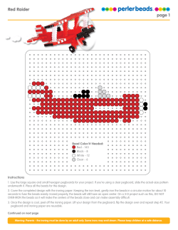


© Copyright 2026