
Equivalence between the eigenvalue problem of non
Equivalence between the eigenvalue problem of non-commutative
harmonic oscillators and existence of holomorphic solutions of Heun
differential equations, eigenstates degeneration and the Rabi model
Masato Wakayama
April 2, 2015
Abstract
The initial aim of the present paper is to provide a complete description of the eigenvalue
problem for the non-commutative harmonic oscillator (NcHO), which is defined by a (two-by-two)
matrix-valued self-adjoint parity-preserving ordinary differential operator [28], in terms of Heun’s
ordinary differential equations, the second order Fuchsian differential equations with four regular
singularities in a complex domain. This description has been achieved for odd eigenfunctions
in Ochiai [25] nicely but missing up to now for the even parity, which is more important from
the viewpoint of determination of the ground state of the NcHO. As a by-product of this study,
examining the monodromy data (characteristic exponents, etc.) of the Heun equation, we prove that
the multiplicity of the eigenvalue of the NcHO is at most two. Moreover, we give a condition for the
existence of a finite-type eigenfunction (i.e. given by essentially a finite sum of Hermite functions)
for the eigenvalue problem and an explicit example of such eigenvalues, from which one finds
that doubly degenerate eigenstates of the NcHO actually exist even in the same parity. Also, we
determine the possible shape of (so-called) Heun polynomial solutions of the Heun equations, which
are obtained by the eigenvalue problem of the NCHO corresponding to finite-type eigenfunctions.
Furthermore, as the second purpose of this paper, we discuss a connection between the quantum
Rabi model [15, 2, 20, 41] and a certain element of the universal enveloping algebra U(sl2 ) of the
Lie algebra sl2 naturally arising from the NcHO through the oscillator representation. Precisely,
an equivalent picture of the quantum Rabi model drawn by a confluent Heun equation is obtained
from the Heun operator defined by that element in U(sl2 ) under a (flat picture of non-unitary)
principal series representation of sl2 through an appropriate confluent procedure.
2010 Mathematics Subject Classification: Primary 34L40, Secondary 81Q10, 34M05, 81S05.
Keywords and phrases: non-commutative harmonic oscillators, universal enveloping algebra,
Heun differential equation, monodromy representation, quantum Rabi model, confluence process.
1
Introduction
In recent years, special attention has been paid to studying the spectrum of self-adjoint operators
with non-commutative coefficients, in other words, interacting quantum systems, like the quantum
Rabi model, the Jaynes-Cumming (JC) model [15], etc., not only in mathematics [7, 8] but also in
theoretical physics [20, 4, 2, 38] and experimental physics ([24, 5], see also e.g. [6]). For instance,
the quantum Rabi model [33] is known to be the simplest model used in quantum optics to describe
interaction of light and matter and the JC model is the widely studied rotating-wave approximation
of the Rabi model [20, 8]. Further, in [24, 5], the authors succeeded in reaching ultra strong coupling
regime in the so-called circuit QED. It shows that their experimental results can be described by
the quantum Rabi model, though it cannot be done by the JC model. The non-commutative
harmonic oscillator (NcHO [28]) Q defined below has been expected to share/provide one of these
Hamiltonians describing such quantum interacting systems.
The purposes of this paper are, in short, providing explicit descriptions of i) the eigenvalue
problem of NcHO in terms of Heun’s differential equations, ii) the degeneration of eigenvalues
1
2
M. Wakayama
and concrete examples together with presenting their possible shape in the Heun picture (Heun
polynomials), and iii) a connection between the NcHO and quantum Rabi model through the
confluence process of Heun’s ODE using representation theory of the three dimensional simple Lie
algebra sl2 .
The normal form the Hamiltonian Q(α,β) (x, D) of NcHO ([31, 32, 28]) is given by
1 2
d
1
1 d2
+ x +J x
+
,
Q(α,β) (x, D) = A −
2 dx2
2
dx 2
where the mutually non-commuting (in general) coefficients A and J are given by
α 0
0 −1
A=
, J=
.
0 β
1 0
From the definition, Q(α,β) (x, D) is obviously a parity-preserving differential operator. We
assume that α, β > 0 and αβ > 1 throughout the paper.
The former requirement α, β > 0 comes from the formal self-adjointness of the operator Q(α,β) (x, D)
relative to the natural inner product on L2 (R, C2 )(= C2 ⊗ L2 (R)). To be more precise, one realizes
Q(α,β) (x, D) as an unbounded operator Q = Qα,β in L2 (R, C2 ) with the dense domain
D = Dα,β := {u ∈ L2 (R, C2 ) | Q(α,β) (x, D)u ∈ L2 (R, C2 )}
such that Qu = Q(α,β) (x, D)u (u ∈ D), where Q(α,β) (x, D)u is understood in the distribution sense.
Hence Q is the so-called maximal operator (associated with Q(α,β) (x, D)). By the global pseudo
differential calculus due to L. H¨
ormander, one sees that Q|S(R,C2 ) = Q, that is, Q is the closure in
the graph-norm of its restriction to the Schwartz space S(R, C2 ) (see [28, 29]). The latter condition
αβ > 1 guarantees the operator Q(α,β) (x, D) is globally elliptic so that Q is self adjoint in D. In
the globally elliptic case, one has D = B 2 (R, C2 ), where for s ∈ R, B s (Rn , CN ) = B s (Rn ) ⊗ CN ,
the spaces B s (Rn ) being the global spaces tailored to the s-th powers of the harmonic oscillator
d2
2
P (x, D) := 21 (− dx
2 +x ) introduced in [36] (see §3 in [28] in details). Since the resolvent is compact,
due to the compact embedding of the space B 2 (R, C2 ), the spectrum is made of a sequence of
eigenvalues diverging to +∞ with finite multiplicities, with eigenfunctions belonging to the Schwartz
class, whence in particular those space are finite dimensional. Thus, from the assumptions, one
concludes that the eigenvalues of the eigenvalue problem Qϕ = λϕ (ϕ ∈ L2 (R, C2 )) are all positive
and form a discrete set with finite multiplicity. One remarks also that the operators considered
here are globally elliptic, and no essential spectrum can therefore be present when they are realized
as self-adjoint operators on the maximal domain. In other words, to have essential spectrum one
has to destroy global ellipticity, and an example is given when α = β = 1 and generalized also
recently to the cases αβ = 1 [30].
It should be first noted that, Q is unitarily equivalent to a couple of quantum harmonic
√ oscillators
when
[A,
J]
=
0,
i.e.
α
=
β
holds,
whence
the
eigenvalues
are
explicitly
calculated
as
α2 − 1 n +
1
2 | n ∈ Z≥0 having multiplicity 2 ([32]). Actually, when α = β, there exists a structure behind Q
corresponding to the tensor product of the two dimensional trivial representation and the oscillator
representation [11] of the Lie algebra sl2 ([32]). However, when α 6= β, representation theoretically,
the apparent lack of an operator which commute with Q (second conserved quantity) besides the
Casimir operator, the image of generator of the center ZU(sl2 ) of the universal enveloping algebra
U(sl2 ) of the Lie algebra sl2 . (Moreover, it has been shown that there is no annihilation/creation
operators associated to NcHO [29] when α 6= β.) Therefore, the clarification of the spectrum in the
general case where α 6= β is considered to be highly non-trivial (see [13, 27, 9], also references in [28]).
It is, nevertheless, worth noticing that the spectral zeta function of Q [12] (which is essentially given
by the Riemann zeta function if α = β) yields a new number theoretic study including the subjects
such as Ap´ery-like numbers, elliptic curves, modular forms, Eichler integrals, Eichler cohomology
groups and their natural generalization (see [16, 17, 18] and references therein, [19], and the recent
study [22]).
We have constructed the eigenfunctions and eigenvalues [32] in terms of continued fractions
determined by a certain three terms recurrence relation, which can be derived from the expansion
of eigenfunctions relative to a basis constructed by suitably twisting the classical Hermite functions.
Eigenvalue problem of the NcHO and Heun’s ODE, and quantum Rabi’s model
We say that the eigenfunction ϕ(x) in L2 (R, C2 ) is of a finite-type if ϕ(x) can be expanded by a
finite number of this Hermite basis. The eigenvalue corresponding to the finite-type eigenfunction is
said to be of finite-type. Otherwise, we say that the eigenvalues/eigenfunctions are of infinite-type.
We denote Σ0 (reps. Σ∞ ) the set of eigenvalues corresponding to eigenfunctions of finite (reps.
infinite)-type. Since the operator Q preserves the parity, we define Σ± to be the set of eigenvalues
whose eigenfunctions are even/odd, that is, those satisfying ϕ(−x) = ±ϕ(x). Then there is a
±
±
classification of eigenvalues: Σ±
(resp. Σ±
∞ = Σ∞ ∩ Σ ) corresponding to even/odd
0 = Σ0 ∩ Σ
±
eigenfunctions of finite (resp. infinite) -type. In [32], it is shown that Σ±
0 ⊂ Σ∞ and the multiplicity
−
of each λ ∈ Σ+
(resp.
Σ
)
is
at
most
2.
This
means
that
once
the
eigenvalue
degenerates in the
∞
∞
−ax2
same parity, one of the eigenfunction is of√the form p(x) × e
, p(x) being a polynomial and a a
positive constant depending on the value αβ − 1, and this resembles the situation of the (doubly)
degenerating eigenvalues case for the quantum Rabi model [20] (see also [2, 37, 41]). The spectral
analysis of the quantum Rabi model seems to be much simpler than the one of NcHO, while the
latter seems to share certain interesting properties the former has. Actually, one finds that the
NcHO gives essentially the quantum Rabi model through the confluence limit procedure at the
stage of Heun equations’ picture (see §5).
It is known [23] that the eigenvalues of NcHO build a continuous curve with arguments α and β.
It comes as an important problem to analyze the behavior of eigenvalue curves, in particular, a main
issue of present day research, especially in mathematical physics, addresses the characterization of
crossing/avoided crossing of eigenvalue curves (see e.g. [35, 7, 8]). From the observation in [23],
−
since the eigenvalue curves are continuous, one can observe that Σ+
∞ ∩ Σ∞ 6= ∅ (see Figure 1 in [23],
p.648; the graph of eigenvalue curves is drawn with respect to the variable s = β/α with a fixed α;
−
+
−
α = 3.0). However, one does not know whether Σ+
0 ∩ Σ∞ (resp. Σ0 ∩ Σ∞ ) is empty or not, while it
+
−
is shown in [32] that Σ0 ∩ Σ0 = ∅. Therefore, the multiplicity of eigenvalue is at most 3 and may
a priori reach 3. In this paper, we will solve one of the longstanding problems for the eigenstate
−
−
+
degeneration of NcHO, in particular, prove that Σ+
0 ∩ Σ∞ = Σ0 ∩ Σ∞ = ∅ (Theorem 1.2).
Generally, in harmonic analysis on the real line, even/odd eigenspaces have completely analogues
structures. Also, in view of the description of the lowest eigenvalue, the study on even eigenstates
is more important [9]. Moreover, we could not see any difference between the even/odd eigenspaces
in the papers [31, 32]. However, in the complex domain picture drawn in [25], the odd part Σ−
corresponds to the second order equation given by Heun’s ordinary differential equation whereas
the even part Σ+ corresponds to the third-order equation (constructed by the same Heun operator).
Therefore, working out a solution to this asymmetry has been desirable for a long time. In this
paper, we prove that there exists a completely parallel structure of even eigenfunctions to that of
the odd eigenfunctions. For readers’ convenience we state the results for the odd case obtained in
[25] in a parallel way. In fact, one of the main techniques to derive this correspondence is based on
a brilliant idea developed in [25], but employing a modified Laplace transform different from that
in [25] which provides an (exact) intertwiner for the oscillator representation corresponding to the
even parity (see §2.2). The reason why one could not obtain in [25] the proper Heun operator (only
the third order operator) in the even case is that the restriction of the modified Laplace transform
in [25] to the even parity has only quasi-intertwing property, that is, there is an extra term which
breaks the U(sl2 )-equivariant actions (see Lemma 2.2).
In conclusion, we are able to show that there exists a second-order Fuchsian differential operator
H(w, ∂w ) so that the eigenvalue problem Qϕ = λϕ (ϕ ∈ L2 (R, C2 )) of the NcHO is equivalent to
the existence of holomorphic solutions f (w) of the differential equation H(w, ∂w )f (w) = 0 on a
suitably chosen domain. Technically speaking, since the eigenspaces of Q are finite dimensional,
they coincide with their topological closure and the same should apply the counterpart of the Heun
operators via this equivalence. With this understanding one can state the first main result as
follows.
Theorem 1.1. There exist linear bijections:
Even :
∼
{ϕ ∈ L2 (R, C2 ) | Qϕ = λϕ, ϕ(−x) = ϕ(x)} −→ {f ∈ O(Ω) | Hλ+ f = 0},
∼
Odd : {ϕ ∈ L2 (R, C2 ) | Qϕ = λϕ, ϕ(−x) = −ϕ(x)} −→ {f ∈ O(Ω) | Hλ− f = 0},
where Ω is a simply-connected domain in C (w-space) such that 0, 1 ∈ Ω while αβ 6∈ Ω, O(Ω)
denotes the set of holomorphic functions on Ω, and Hλ± = Hλ± (w, ∂w ) are the Heun ordinary
3
4
M. Wakayama
differential operators given respectively by
Hλ+ (w, ∂w )
d2
+
:=
dw2
Hλ− (w, ∂w )
d2
+
:=
dw2
1
2
− p − 21 − p
p+1
+
+
w
w−1
w − αβ
and
p + 23
1−p
−p
+
+
w
w − 1 w − αβ
!
!
− 12 p + 12 w − q +
d
+
dw w(w − 1)(w − αβ)
(1.1)
− 32 pw − q −
d
+
.
dw w(w − 1)(w − αβ)
(1.2)
Here the numbers p = p(λ) and ν = ν(λ) are defined thorough the following relations:
p
αβ(αβ − 1)
2ν − 3
p=
, λ = 2ν
.
4
α+β
(1.3)
The accessory parameters q ± = q ± (λ) in these Heun’s operators are expressed by the parameters
α, β and eigenvalue λ as
n
1
1
3 2 β − α 2 o
1 2 (αβ − 1) −
p+
,
(1.4)
− p+
q+ =
p+
2
4
β+α
2
2
o
n
3
3 2 β−α 2
(αβ − 1) − p.
q − = p2 − p +
(1.5)
4
β+α
2
Remark 1.1. Since the Fuchsian operators Hλ± (w, ∂w ) have regular singulars (only) at the points
0, 1 and αβ, the general theory (see e.g. [34]) indicates that the connected simply-connected open
subset Ω(∈ C) in Theorem 1.1 can be chosen arbitrary provided it satisfies 0, 1 ∈ Ω, αβ 6∈ Ω. For
instance, Ω can be taken to be an open disk of radius (1 + αβ)/2 centered at the origin. See also
the discussion in §3.2.
Remark 1.2. The bijections in the theorem are essentially constructed by the extension of the
map TC : L2 (R)fin → C[y] defined in §2.1 (see (2.1)) to their completion L2 (R) → C[y] (see
Remark 2.3) and the modified Laplace operator L1 (Even case) and L2 (Odd case), respectively in
§2.2. Concerning the L2 -condition and the holomorphic condition for the solutions of the Fuchsian
differential equation with 6 regular singularities, which is equivalent to our Heun’s ODE obtained by
the variable change w = (constant) × z 2 , see §3.2. Summarizing those discussions done in advance,
we shall put the proof of Theorem 1.1 in §3.3.
In this paper, the canonical form of Heun’s equations are taken as
!
d2
γ
δ
d
ρµw − q
+
+
+
+
.
(1.6)
dw2
w w − 1 w − t dw w(w − 1)(w − t)
The parameters γ, δ, , ρ, µ are generally complex and arbitrary, except that t 6= 0, 1. The first five
parameters are linked by the equation
γ + δ + = ρ + µ + 1.
(1.7)
The equation (1.6) is of Fuchsian type with regular singularities at w = 0, 1, t, ∞ and the characteristic exponents (or Frobenius exponents) at these regular singularities are given by {0, 1 − γ},
{0, 1 − δ}, {0, 1 − } and {ρ, µ} respectively. (The characteristic exponents are the roots of the
indicial equation at the regular singularity [34].) As shown in (1.7), the sum of these exponents
must take the value 2 according to the general theory of Fuchsian equations. The Riemann schema
puts the equation (1.6) in the form (of a Riemann P -symbol)
0
1
t
∞ ;w q
0
.
0
0
ρ
(1.8)
1−γ 1−δ 1− µ
The number q represents the accessory parameter. It sometimes plays the part of an eigenparameter.
As to the general theory of Heun ODEs and Riemann’s scheme, see §1.1 and Appendix 7 in [34]
(also [14, 35]).
Eigenvalue problem of the NcHO and Heun’s ODE, and quantum Rabi’s model
5
We note that the Heun operators Hλ± (w, ∂w ) in the theorem above have four regular singular
points, w = 0, 1, αβ and ∞. Hence, the respective Riemann’s scheme of the operators Hλ± (w, ∂w )
are expressed as
0
1
αβ
∞
; w q+
1
0
0
0
(1.9)
H+
λ :
2
3
1
1
p + 2 p + 2 −p − p + 2
and
0
0
H−
:
λ
p
1
0
p+1
αβ
0
−p −
∞
1
2
; w q−
3
2
.
(1.10)
−p
One notes that each element of the first row indicates a regular singular point of Hλ± and those in
the second and third rows are expressing the corresponding exponents.
As a corollary of this theorem we may actually provide examples of finite-type eigenvalues (and
corresponding solutions). In other words, we have an even (resp. odd) polynomial solution when
the parameter p + 12 ∈ N (resp. p ∈ N) satisfies a certain algebraic equation obtained by the
determinant of Jacobi’s (i.e. tri-diagonal) matrix (Proposition 4.1). It is also worth noticing that
the ground state of the NcHO consists of only even functions [10], whence its simplicity follows
from the result in [39]. The criterion for this simplicity (Theorem 1.1 in [39]) can be proved also
by Theorem 1.1 above together with an upper bound estimate of the lowest eigenvalue given in
[28] (Theorem 8.2.1) (see [39]). Furthermore, combining the results in Theorem 1.1 for even and
odd eigenfunctions, and examining the monodromy data (characteristic exponents, etc.) of the
corresponding Heun differential equations, we will show the following.
Theorem 1.2. Suppose αβ > 1. The multiplicity mλ of the eigenvalue λ for the non-commutative
harmonic oscillators Q is at most 2. Moreover, when α =
6 β, mλ = 2 holds if and only if either of
the following two cases holds:
−
1. λ ∈ Σ+
0 (resp. Σ0 ); in this case one has a unique (up to scalar multiples) finite-type solution,
i.e., a finite linear combination
of even (resp. odd)
√
√ twisted Hermite functions. Moreover, λ
is of the form λ = 2
αβ(αβ−1)
(2L
α+β
+ 21 ) (resp. 2
αβ(αβ−1)
(2L
α+β
+ 32 )) for L ∈ N,
−
2. λ ∈ Σ+
∞ ∩ Σ∞ .
Remark 1.3. As for the precise definition of twisted Hermite functions in Theorem 1.2, see [32].
Figure 1: Examples of configuration for doubly degenerations of the spectrum of NcHO
Furthermore, employing the analogous discussion developed in [26], that is, using monodromy
representation, in §4.3, we will determine the shape of the Heun polynomial solutions, which are
the solutions of the Heun equations Hλ± f = 0 derived from the eigenvalue problems of the NCHO
(by Theorem 1.1) corresponding to finite-type eigenfunctions.
In the final section, we will discuss a connection between the operator R (a degree 2 element
of the universal enveloping algebra U(sl2 )) obtained naturally from NcHO through the oscillator
representation of sl2 (see Lemma 2.1) and the quantum Rabi model. Although the quantum Rabi
6
M. Wakayama
model has had an impressive impact on many fields of physics [6], only recently (in 2011) could
this model be declared solved by D. Braak [2]. The Hamiltonian is given as
HRabi /~ = ωa† a + ∆σz + g(σ + + σ − )(a† + a),
with σ ± = (σx ± iσy )/2 (see §5), by taking the confluence procedure of Heun’s equation (see
[35, 34]). Actually, employing a (flat picture of) principal series representation $a of sl2 (see
Lemma 2.3), which is inequivalent to the oscillator representation when a 6= 1, 2 that gives the
NcHO, one constructs the confluent Heun differential operator corresponding to the quantum Rabi
model from R. The result in §5 amounts to saying that the Rabi model is considered to be a sort
of confluent version of the NcHO. We shall suppose throughout that αβ > 1.
2
Representation theoretic setting
2.1
Oscillator representation of sl2
Although there is no exact (continuous) symmetry on Q (α 6= β) described by the Lie algebra sl2 ,
as it is the case for the quantum harmonic oscillator, there seems to exist still a vague hidden (or
modified) sl2 -symmetry behind it, beside the parity Z2 . Thus a formulation of the problem by the
language of sl2 is useful, as we have observed in [31, 32, 25]. Moreover, as we will see in §5, in order
to observe the relation between the NcHO and the Rabi model, a viewpoint employing Lie algebra
representation (e.g. [21, 11]) of sl2 is important.
Let H, E and F be the standard generators of the Lie algebra sl2 defined by
1 0
0 1
0 0
H=
, E=
, F =
.
0 −1
0 0
1 0
They satisfy the commutation relations
[H, E] = 2E, [H, F ] = −2F, [E, F ] = H.
For the triplet (κ, ε, ν) ∈ R3>0 , define a second order element R of the universal enveloping
algebra U(sl2 ) of sl2 by
i
o
2 nh
(sinh 2κ)(E − F ) − (cosh 2κ)H + ν (H − ν) + (εν)2 ∈ U(sl2 ).
R :=
sinh 2κ
˜ by
Define also an element R
h
i
o
2 n
˜=
R
(H − ν) (sinh 2κ)(E − F ) − (cosh 2κ)H + ν + (εν)2 ∈ U(sl2 ).
sinh 2κ
We define the oscillator representation π of sl2 by
π(H) = x∂x + 1/2, π(E) = x2 /2, π(F ) = −∂x2 /2,
where ∂x = d/dx. We will also denote the algebra homomorphism from the universal enveloping
algebra U(sl2 ) to the ring C[x, ∂x ] of differential operators by the same letter π. By this realization,
the eigenvalue problem Qϕ(x) = λϕ(x) (ϕ ∈ L2 (R, C2 )) turns to be solving the following equation.
[Aπ(E + F ) + Jπ(H) − λI]ϕ(x) = 0.
As we have shown in [32] (see also [25]) this equation can be rewritten as
1
˜
= 0,
[π(E + F ) + √ Jπ(H) − λA−1 ]ϕ(x)
αβ
1
where ϕ(x)
˜
= A 2 ϕ(x).
Now, as usual, let us realize the oscillator representation
on the polynomial ring C[y] in place
1
1
of L2 (R) using the Cayley transform C := √12
.
−1 1
Eigenvalue problem of the NcHO and Heun’s ODE, and quantum Rabi’s model
√
√
Define the annihilation operator ψ = (x + ∂x )/ 2 and creation operator ψ † = (x − ∂x )/ 2.
2
Then one has [ψ, ψ † ] = 1. Put ϕ0 (x) := e−x /2 ∈ L2 (R). Then ϕ0 is the vacuum vector, that is,
ψϕ0 = 0, and ϕ0 gives the ground state of the quantum harmonic oscillator H := ψ † ψ + 12 . We
define in general ϕn := (ψ † )n ϕ0 , the√Hermite functions. Then the set {ϕn | n = 0, 1, 2, . . .} forms
an orthogonal basis with (ϕn , ϕn ) = πn!, ( , ) being the standard inner product of L2 (R) (see e.g.
[11]). We denote the set of all finite linear combinations of the Hermite functions ϕn by L2 (R)fin .
Let
TC : L2 (R)fin → C[y]
(2.1)
be the linear map defined by the property TC (ϕn ) = y n . Then one immediately sees that TC (ψ † ϕ) =
yTC (ϕ) and TC (ψϕ) = ∂y TC (ϕ). Then, if we define the representation (π 0 , C[y]) of sl2 by
π 0 (H) = y∂y + 1/2, π 0 (E) = y 2 /2, π 0 (F ) = −∂y2 /2,
−1
one may easily show that π 0 (CXC
)TC = TC π(X) (X ∈ sl2 ). Moreover, if we define a Fisher√inner
√
g (y))|y=0 (f, g ∈ C[y]), one finds that (y m , y n )F = δm,n πn!,
product on C[y] by (f, g)F = π(f (∂y )¯
whence TC gives an isometry. If we denote the completion of C[y] with respect to this inner product
by C[y], then it follows that the map TC can be extended to an isometry between the Hilbert spaces
L2 (R) and C[y].
The first claim of the following lemma follows immediately from [25] (Corollary 9 with Lemma
8), which translates the eigenvalue problem of Q into a single differential equation. The second
follows in a similar way.
Lemma 2.1. Assume α 6= β. Determine the triplet (κ, ε, ν) ∈ R3>0 by the formulas
s
cosh κ =
α − β αβ
1
α+β
, ε=
λ.
, sinh κ = √
, ν = p
αβ − 1
α+β
αβ − 1
2 αβ(αβ − 1)
Then the eigenvalue problem Qϕ = λϕ (ϕ ∈ L2 (R, C2 )) is equivalent
to the equation π 0 (R)u =
0 1
0 (u ∈ C[y]) by the isometry TC : L2 (R) → C[y]. Let K =
∈ Aut(C2 ⊗ L2 (R)). Then the
1 0
˜ = 0 (u ∈
eigenvalue problem KQKϕ = λϕ (ϕ ∈ L2 (R, C2 )) is equivalent to the equation π 0 (R)u
C[y]).
Remark 2.1. We remark that the twist KQK and Q have the same spectrum.
Remark 2.2. Notice that π 0 (R) is a 3rd order differential operator and the recurrence equation (or
its corresponding continued fraction) in [32] is equivalent to this third order differential equation.
It is also worth noting that the construction of the transcendental function G± (x) whose zeros give
regular eigenvalues of the quantum Rabi model in [2, 3] resembles that of NcHO in [32].
Remark 2.3. The correspondence ϕ ↔ u in the lemma above can be given explicitly. For the
readers’ convenience, we briefly summarize the correspondence given in [25].
Put
i
S± := E + F ± √ H ∈ sl2
αβ
and
1 1
ϕ˜ := √
2 1
√
−i
α
i
0
√0 ϕ.
β
Define (invertible) maps T : L2 (R) → L2 (R) and T 0 : C[y] → C[y] by
(T f )(x) = e
i(sinh κ)x2 /2
1/4
(cosh κ)
√
f ( cosh κ x)
and
r cosh κ
y .
(T g)(y) = g
i − sinh κ
0
The map T preserves the standard inner product on L2 (R) (and intertwines the actions of sl2 , see
p.361 in [25]). Also T 0 preserves the (Fisher) inner product on C[y] and can be extended to the
7
8
M. Wakayama
isometry (using the same letter) T 0 : C[y] → C[y] (see, p.363 in [25]). Regarding T (resp. T 0 ) as an
isometry on L2 (R, C2 ) = C2 ⊗ L2 (R) (resp. C2 ⊗ C[y]) in an obvious way, we set
u
:= T 0 TC T ϕ.
˜
u
˜
Then one knows that whenever α 6= β the eigenvalue problem Qϕ = λϕ can be written as
"
# α+β
α+β
1
0
π
(H)
−
λ
−
ελ
u
cosh κ
2αβ
2αβ
= 0.
α+β
1
0
u
˜
− α+β
ελ
π
((cosh
2κ)H
−
(sinh
2κ)(E
−
F
))
−
λ
2αβ
cosh κ
2αβ
A standard
argument allows us to see that the system of differential equations above for the vector
u
function
is equivalent to the single differential equation for u
u
˜
"
n
#
α + β on 1
α + β o n α + β o2
1
0
0
u = 0,
π ((cosh 2κ)H−(sinh 2κ)(E−F ))−
λ
π (H)−
λ −
ελ
cosh κ
2αβ
cosh κ
2αβ
2αβ
by putting
2αβ h
u
˜=
(α + β)ε
r
1−
1 0
α+β i
π (H) −
λ u.
αβ
2αβ
Therefore, rewriting the above single equation, one concludes that Qϕ = λϕ (ϕ ∈ L2 (R, C2 )) is
equivalent to the equation π 0 (R)u = 0 (u ∈ C[y]) (Lemma 8 and Corollary 9 in [25]).
2.2
Quasi-intertwiners arising from Laplace transforms
In order to obtain a complex analytic picture of the equation π 0 (R)u = 0 in Lemma 2.1 and to
observe a connection between the NcHO and the quantum Rabi model through Heun’s ODE, we
introduce two representations of sl2 .
Let a ∈ N. Define first the operator Ta acting on the space of Laurent polynomials C[y, y −1 ]
(or y 2 C[y]) by
1
(a − 1)(a − 2) 1
Ta := − ∂y2 +
· 2.
2
2
y
Define a modified Laplace transform La by
Z
(La u)(z) =
∞
u(yz)e−
y2
2
y a−1 dy.
0
Then, one finds that
(La Ta u)(z) = −
1
a − 1
1
a−1
∂z +
(La u)(z) + u0 (0)δa,1 −
u(0)δa,2 ,
2z
2z 2
2z
2z 2
where δa,k = 1 when k = a and 0 otherwise. This can be true whenever u(0), u0 (0) and (La u)(z)
exist.
We now define a representation πa0 of sl2 on y a−1 C[y] by
πa0 (H) = π 0 (H), πa0 (E) = π 0 (E), πa0 (F ) = Ta = π 0 (F ) +
(a − 1)(a − 2) 1
· 2.
2
y
(2.2)
Next, introduce another representation of sl2 on C[z, z −1 ] by
1
1
1
a−1
.
$a (H) = z∂z + , $a (E) = z 2 (z∂z + a), $a (F ) = − ∂z +
2
2
2z
2z 2
Then one verifies the following
(2.3)
Eigenvalue problem of the NcHO and Heun’s ODE, and quantum Rabi’s model
Lemma 2.2.
9
(i) Let a 6= 1, 2. Then one has
La πa0 (X) = $a (X)La (X ∈ sl2 ).
Furthermore, when a = 1 (resp. a = 2) the restriction of L1 (resp. L2 ) to the space of
even (resp. odd) functions turns out to be an intertwiner between the two representations
π 0 (= π10 ) (resp. = π20 )) and $1 (resp. $2 ). Precisely, Lj (j = 1, 2) possesses the following
quasi-intertwining property:
Lj π 0 (X)
= $j (X)Lj , (for X = H, E),
0
= $1 (F )(L1 u)(z) + u0 (0)/(2z),
0
= $2 (F )(L2 u)(z) − u(0)/(2z 2 ).
(L1 π (F )u)(z)
(L2 π (F )u)(z)
n
PN
n+a
n
(ii) The map La gives y n 7→ 2 2 −1 Γ n+a
z , whence if u(y) =
∈ C[y] then
n=0 un y
2
√
P
a
N
n+a
n
−1
(
2z)
.
u
Γ
(La u)(z) = 2 2
n=0 n
2
(iii) If we define the inner product √( , )a in z-space such that {z n | n ∈ Z+ } forms an orthogonal
πn!
2 , then the modified Laplace transform La defines an
system and (z n , z n )a =
n+a
2n+a−2 Γ
2
isometry. For instance, when a = 1, 2, the inner products are given by (z n , z n )1 =
p
√
Γ( n+1 )
2n and (z n , z n )2 = Γ( n 2+1) ∼ 2/n as n → ∞, respectively.
2Γ( n
2 +1)
Γ( n+1
2 )
∼
2
Proof. By the definition (2.2) (resp. (2.3)) of the representation πa0 (resp. $a ), integral by parts
at the definition of the Laplace integral La shows the assertion (i). Straight forward computation
and the Stiring formula show (ii) and (iii).
Since $a (E)z −a = 0, one has the following second equivalence: the representation (πa0 , y 2−a C[y 2 ])
can be considered as the Langlans quotient of the representations ($a , C[z 2 , z −2 ]) or ($a , zC[z 2 , z −2 ])
depending on the parity of a.
Lemma 2.3. The operator La gives the equivalence of irreducible modules of sl2 :
(πa0 , y a−1 C[y 2 ]) ∼
= ($a , z a−1 C[z 2 ]),
∼ ($a , z a C[z 2 , z −2 ]/z −a C[z −2 ]).
(πa0 , y 2−a C[y 2 ]) =
Moreover, the Casimir operator ZC := 4EF + H 2 − 2H ∈ ZU(sl2 ) takes the value (a − 1)(a − 2) − 34
in both representations (πa0 , y a−1 C[y 2 ]) and (πa0 , y 2−a C[y 2 ]).
Remark 2.4. The lemma holds for a = 1, 2. Actually, for instance, by the quasi-intertwiner L1 , we
obtain the equivalence between the odd part of the (oscillator) representation (π 0 , yC[y 2 ]) and the
Langlands quotient of the representation ($, zC[z 2 , z −2 ]) of sl2 .
Remark 2.5. There is a symmetry a ↔ 3 − a for πa0 . Actually, when a 6∈ Z, there is an equivalence
0
between the two representations πa0 and π3−a
in a suitable setting.
2.3
Heun differential operators
Recalling the operator R ∈ U(sl2 ), one observes (with θz = z∂z ) that
n
1
1
2ν o
1
2(εν)2
$a (R) = (z 2 + z −2 − 2 coth 2κ)(θz + ) + (a − )(z 2 − z −2 ) +
(θz + − ν) +
.
2
2
sinh 2κ
2
sinh 2κ
Also, one notes that
n
o 2(εν)2
˜ = (θz + 1 − ν) (z 2 + z −2 − 2 coth 2κ)(θz + 1 ) + (a − 1 )(z 2 − z −2 ) + 2ν
$a (R)
+
.
2
2
2
sinh 2κ
sinh 2κ
˜ is
Therefore, conjugating by z a−1 , one obtains the following lemma for R. The formula for R
similar.
10
M. Wakayama
Lemma 2.4. For each integer a, one has
n
1
z −a+1 $a (R)z a−1 = (z 2 + z −2 − 2 coth 2κ)(θz + a − )
2
o
1
2ν
2(εν)2
1 2
(θz + a − − ν) +
.
+(a − )(z − z −2 ) +
2
sinh 2κ
2
sinh 2κ
Furthermore, notice that the operators $a (H), $a (E) and $a (F ) are invariant under the symmetry z → −z. This implies that the operator $a (R) can be expressed in terms of the variable z 2 .
In fact, one has the following.
Proposition 2.5. Let w := z 2 coth κ. Then the following relation holds.
z −a+1 $a (R)z a−1 = 4(tanh κ) w(w − 1)(w − coth2 κ)H a (w, ∂w ),
where H a (w, ∂w ) is the Heun differential operator given by
d2
+
H (w, ∂w ) =
dw2
a
3 − 2ν + 2a −1 − 2ν + 2a
−1 + 2ν + 2a
+
+
4w
4(w − 1)
4(w − coth2 κ)
1
+2
(a − 12 )(a −
1
2
− ν)w − qa
w(w − 1)(w − coth2 κ)
!
d
dw
.
Here the appearing accessory parameter qa is given by
qa =
n
− (a −
o
1
1
1
− ν)2 + (εν)2 (coth2 κ − 1) − 2(a − )(a − − ν).
2
2
2
˜ one has z −a+1 $a (R)z
˜ a−1 = 4(tanh κ) w(w − 1)(w − coth2 κ)H
˜ a (w, ∂w ) with
Similarly, for R,
!
2
d
f
−1
−
2ν
+
2a
3
−
2ν
+
2a
3
+
2ν
+
2a
d
˜ λa (w, ∂w ) =
H
+
+
+
2
dw2
4w
4(w − 1)
dw
4(w − coth κ)
1
+2
(a − 21 )(a +
3
2
− ν)w − qa
w(w − 1)(w − coth2 κ)
.
Proof. Since w = z 2 coth κ, one notices that z∂z = 2w∂w . Put t = coth2 κ for simplicity. Using the
relations
z 2 + z −2 − 2 coth 2κ = (tanh κ)w−1 (w − 1)(w − coth2 κ),
z 2 − z −2 = (tanh κ)w−1 (w2 − coth2 κ),
2/ sinh 2κ = (tanh κ)(coth2 κ − 1),
one obtains
h
1
z −a+1 $a (R)z a−1 =(tanh κ) w−1 (w − 1)(w − t)(2w∂w + a − )
2
i
1
1
+(a − )w−1 (w2 − t) + (t − 1)ν (2w∂w + a − − ν) + (t − 1)(εν)2 .
2
2
Taking into account the relation [∂w , w] = 1, one observes
z −a+1 $a (R)z a−1
h
2
=(tanh κ) 4w(w − 1)(w − t)∂w
+ (2a − 2ν + 3)(w − 1)(w − t) + (2a − 2ν − 1)w(w − t) + (2a + 2ν − 1)w(w − 1) ∂w
i
1
1
1
1
1
+2w(a − )(a − − ν) + − (a − − ν)2 + (εν)2 (t − 1) − 2(a − )(a − − ν) .
2
2
2
2
2
Eigenvalue problem of the NcHO and Heun’s ODE, and quantum Rabi’s model
11
Factoring out the leading coefficient, one obtains the expression of H a (w, ∂w ). The expression of
˜ a (w, ∂w ) follows from the relation
H
λ
˜ a−1 − z −a+1 $a (R)z a−1
z −a+1 $a (R)z
#
"
n 1
a − 12
1
1 o
2
+
.
=4(tanh κ) w(w − 1)(w − coth κ) − +
+
w w−1 w−t
(w − 1)(w − t)
This proves the proposition.
3
Heun’s operators description for NcHO
3.1
Equivalence of differential operators
The equivalence between the spectral problem of Q and the existence/non-existence of holomorphic
solutions of a Heun’s ODE in a certain complex domain is described in [25] for the odd parity. In
the same way we have the equivalence for the even parity.
Proposition 3.1. The element R ∈ U(sl2 ) satisfies the following equations:
(L1 π 0 (R)u)(z)
= $1 (R)(L1 u)(z) + (ν − 23 )u0 (0)z −1 ,
(L2 π 0 (R)u)(z)
= $2 (R)(L2 u)(z) − (ν − 21 )u(0)z −2 .
In particular, the equation (π 0 (R)u)(z) = 0 for the even and odd case is respectively equivalent to
the equation
$1 (R)(L1 u)(z) = 0 (the even case)
and
$2 (R)(L2 u)(z) = 0 (the odd case).
(3.1)
Here
n
o
2(εν)2
2ν
1
= (z 2 + z −2 − 2 coth 2κ)(θz + 12 ) + 12 (z 2 − z −2 ) + sinh
2κ (θz + 2 − ν) + sinh 2κ ,
n
o
2(εν)2
1
2ν
$2 (R) = (z 2 + z −2 − 2 coth 2κ)(θz + 21 ) + 32 (z 2 − z −2 ) + sinh
2κ (θz + 2 − ν) + sinh 2κ ,
$1 (R)
∂
.
where we have put θz = z ∂z
Proof. For each j = 1, 2, the relation between π 0 (R) and $j (R) follows from the quiasi-intertwining
property of the operator Lj resulting from (i) in Lemma 2.2. Since u0 (0) = 0 (resp. u(0) = 0) for
the even (resp. odd) case, the equivalence between the equation (π 0 (R)u)(z) = 0 and (3.1) follows
immediately. The expression of $j (R) in terms of the variable z is obtained by taking j = a = 1, 2
of $a (R) in §2.3.
For the even parity, by Proposition 2.5, one has
p −1
$1 (R) = 4 αβ w(w − 1)(w − αβ)Hλ+ (w, ∂w ),
where Hλ+ (w, ∂w ) := Hλ1 (w, ∂w ) is the Heun differential operator given by (1.1) in the Introduction,
that is,
!
1
1
2
− 12 p + 12 w − q +
−
p
−
−
p
d
p
+
1
d
+
2
2
Hλ (w, ∂w ) =
+
+
+
+
,
dw2
w
w−1
w − αβ dw w(w − 1)(w − αβ)
where
p :=
2ν − 3
4
α+β
(ν = p
λ)
2 αβ(αβ − 1)
and the accessory parameter q + := q1 is given by
n
1 2 3 2 β − α 2 o
1
1
q+ =
p+
− p+
(αβ − 1) −
p+
.
2
4
β+α
2
2
By its expression, Hλ+ (w, ∂w ) is a second-order linear differential operator with four regular singular
points 0, 1, αβ and ∞ on P1 (C). Notice that the parameter ν designates the exponents. From these
observations, we may summarize the properties of the operator $1 (R) as follows.
12
M. Wakayama
Proposition 3.2. The second-order linear differential operator $1 (R) with rational coefficients
1
1
in z has six singular points z = 0, ±(αβ)− 4 , ±(αβ) 4 , ∞. Here, all these six points are of regular
singular type. The exponents of those singularities can be read from the following Riemann scheme:
1
1
1
1
∞
; z q+
0
(αβ)− 4 −(αβ)− 4 (αβ) 4 −(αβ) 4
.
$1 (R) : 0
0
0
0
0
1
3
3
p+ 2
−p
−p
−2p − 1
2p + 1 p + 2
Proof. The former statement is immediate from the discussion above. We prove the latter. By the
expression Hλa (w, ∂w ) in Proposition 2.5 with a = 1, the second-order linear differential operator
Hλ+ (w, ∂w ) with four regular singularities on the Riemann sphere C∪{∞} has the following Riemann
schemes (P -symbols) [34]:
0
1
coth2 κ
∞
; w q+
0
1
coth2 κ ∞ ; w q +
1
.
0
= 0
0
0
ρ
0
0
2
3
1
1
1−γ 1−δ
1−
µ
−p
−p − 2
p+ 2 p+ 2
Since
$1 (R) = 4 coth2 κ z 2 (z 2 − tanh κ)(z 2 − coth κ)Hλ+ (w, ∂w )
√
and tanh κ = 1/ αβ, one sees that the P -symbol of $1 (R) is given by
√
√
0
1/ αβ
αβ
∞
; z2 q+
1
0
.
0
0
2
1
3
1
p+ 2 p+ 2
−p −p − 2
By unfolding z 2 7→ z, we have the assertion.
Remark 3.1. For the readers’ convenience, we recall the Riemann schema of the operator $2 (R)
from [25]:
1
1
1
1
0
(αβ)− 4 −(αβ)− 4
(αβ) 4
−(αβ) 4
∞
; z q−
.
$2 (R) : 1
0
0
0
0
2
1
1
2p + 1
p+1
p+1
−(p + 2 ) −(p + 2 ) −2p − 1
3.2
L2 -conditions and analytic continuation
The discussion of this part is analogues to that one made by Ochiai in [25]. However, in [25], it
was necessary to deal with the third order equation (see Lemma 13 in [25]) because there was no
chance to discuss the even eigenfunctions in the framework of a Heun ODE directly. Here, since we
have taken another modified Laplace integral L1 (in place of L2 ), which intertwines eigenfunctions
of the NCHO in the even parity and formal even power series solutions in z-space directly, it is
sufficient to handle only a second order equation.
We denote by O0 the germ of the holomorphic function at the origin 0. In order to accomplish
the proof of Theorem 1.1, we study the holomorphic even solution u
ˆ(z) := (L1 u)(z) ∈ O0 satisfying
the equation $1 (R)(ˆ
u) = 0 (see (3.1) in Proposition 3.1). We will take the discussion essentially
due to [25], which establishes the relation between L2 -conditions on R (or convergence conditions
in C[y]) and the holomorphic solutions of the equation with regular singularities in z-space.
One first notices that the solution u
ˆ ∈ O0 of $1 (R)(ˆ
u) = 0 can be analytically continued along
a path avoiding the singular points of the differential equation. Namely, in our case, the solution
1
is holomorphic on the open disk of radius (αβ)− 4 (< 1). We now consider the behavior of the
1
solution near the points z = ±(αβ)− 4 . Since the singularities of $1 (R) are located (only) at
1
1
0, ±(αβ)− 4 , ±(αβ) 4 and ∞ as in Proposition 3.2, we have the following two possibilities.
1
1. The solution u
ˆ(z) is holomorphic near the points z = ±(αβ)− 4 . In this case, general theory
guarantees that it is continued to a single-valued holomorphic function on the disk {z ∈
P∞
1
C | |z| < (αβ) 4 }. In terms of the Taylor expansion u
ˆ(z) = n=0 an z 2n , one has then
p
∀ε > 0, ∃N such that ∀n > N,
|an | ≤ (1/ αβ + ε)n .
Eigenvalue problem of the NcHO and Heun’s ODE, and quantum Rabi’s model
13
2. The solution cannot be holomorphically continued to at least one of
points z = ±(αβ)−1/4 ,
Pthe
∞
that is, the the radius of convergence of the Taylor series u
ˆ(z) = n=0 an z 2n is (αβ)−1/4 . In
this case, one has
p
∀ε > 0 and ∀N, ∃n > N such that
|an | ≥ ( αβ − ε)n .
P∞
Proposition 3.3. Consider the (even) formal series solution u(y) = n=0 un y 2n ∈ C[[y]] of the
equation π 0 (R)u = 0. Let u
ˆ(z) := (L1 u)(z) ∈ C[[z]]. Then one has the following.
(i) A formal series solution u
ˆ(z) ∈ C[[z]] of the equation $1 (R)f = 0 converges to a holomorphic
function near the origin 0, that is, u
ˆ(z) ∈ O0 .
(ii) The following conditions are equivalent:
(a) u(y) convergences in the Hilbert space C[y].
(b) u
ˆ(z) converges to a holomorphic function on the unit disk.
(c) u
ˆ(z) can be holomorphically continued to a neighborhood of the closed interval [0, (αβ)−1/4 ].
(iii) The following conditions are equivalent:
(a) u(y) does not convergence in the Hilbert space C[y].
(b) u
ˆ(z) cannot be convergent to any holomorphic function on the unit disk.
(c) u
ˆ(z) cannot be holomorphically continued to a neighborhood of the closed integral [0, (αβ)−1/4 ].
(iv) The unit disk in the statements in (ii) and (iii) can be replaced by a connected and simplyconnected domain Ω0 of C which contains the three points 0, ±(αβ)−1/4 and does not contain
either of ±(αβ)1/4 .
Proof. Since the operator $1 (R) is regular singular at the origin, one has that any formal series
solution of f ∈ C[[z]] of the equation $1 (R)f = 0 converges to a holomorphic function near the
origin, whence the assertion (i) follows.
√
2Γ( n
2 +1)
Recall the fact (z n , z n )1 = Γ( n+1
∼ 2n (n → ∞) on C[[z]] space, which makes L1 an isometry
)
2
1
between C[[y]] and C[[z]]. Setting an = un Γ(n + 12 )2n− 2 , one has |un |2 (y 2n , y 2n ) = |an |2 (z 2n , z 2n )1
when u
ˆ(z) = (L1 u)(z). It follows that the condition (ii-b) and (iii-b) imply
(
2
2n
2n
|un | (y , y )
≤
≥
√
2Γ(n+1)
(1/ αβ
Γ(n+ 21 )
2Γ(n+1) √
( αβ −
Γ(n+ 21 )
+ ε)2n
2n
ε)
for case (ii),
for case (iii).
This immediately shows (ii-b) ⇒ (ii-a) and (iii-b) ⇒ (iii-a). Since there are only two possibilities
for the behavior of u
ˆ(z) as we described above, the converse (ii-a) ⇒ (ii-b) and (iii-a) ⇒ (iii-b)
also follows. The claim (ii-b) ⇒ (ii-c) is obvious. Conversely, since u
ˆ(z) is even, the condition
(ii-c) implies that this is also holomorphic at z = −(αβ)−1/4 . Since u
ˆ(z) is a solution of the
differential equation $1 (R)(ˆ
u) = 0 it can be holomorphically continued to the regular singular
points z = ±(αβ)1/4 . In particular, it is holomorphic on the unit disk. This proves (ii-b). The
same reasoning shows (iii-b) ⇔ (iii-c).
The discussion above shows that the statement in (ii) (resp. (iii)) remains true if one replaces
the unit disk by such domain Ω0 . This proves (iv).
3.3
Proof of Theorem 1.1
We are now in a position to give a proof of Theorem 1.1.
Let Ω0 be a connected and simply-connected domain of C satisfying 0, ±(αβ)−1/4 ∈ Ω0 while
±(αβ)1/4 6∈ Ω0 . Then, to summarize the equivalences of the several equations in question, one has
firstly the equivalence Qϕ = λϕ (ϕ ∈ L2 (R, C2 )) ⇔ π 0 (R)u = 0 (u ∈ C[y]), which is established
in Lemma 2.1 (due to §2 in [25], see Remark 2.3). Successively, by Proposition 3.3, one has the
equivalence π 0 (R)u = 0 (u ∈ C[y]) ⇔ $1 (R)ˆ
u(z) = 0 (ˆ
u ∈ O(Ω0 )) for the even parity under the
intertwining isometry u 7→ u
ˆ = L1 u obtained in Lemma 2.2. It follows that the eigenvalue problem
Qϕ = λϕ of the NcHO for the even parity is equivalent to that of finding all the holomorphic even
solutions U (z) ∈ O(Ω0 ) of the differential equation $1 (R)U (z) = 0.
14
M. Wakayama
Notice that every solution U (z) ∈ √
O(Ω0 ) of $1 (R)U (z) = 0 is the sum of an even solution and
odd solution. By the map z → w = αβ z 2 , the set of even functions in O(Ω0 ) is isomorphic to
O(Ω), where Ω is taken to be a connected and simply-connected domain in w-space containing 0
and 1, but does not contain the point αβ(> 1). Recall also that the differential operator $1 (R) is
in terms of variable w expressed as
$1 (R) = 4
p
αβ
−1
w(w − 1)(w − αβ)Hλ+ (w, ∂w ) : O(Ω) → O(Ω).
(3.2)
It is hence elementary to see the equivalence
ker($1 (R), O(Ω)) ∼
= ker(Hλ+ , O(Ω)).
Therefore, the eigenvalue problem of Q for the even parity is equivalent to finding the holomorphic
solutions f (w) ∈ O(Ω) of the differential equation Hλ+ (w, ∂w )f (w) = 0. This completes the proof
of Theorem 1.1.
Remark 3.2. By the same reasoning of the proof of Lemma 17 in [25], one sees that the map
$1 (R) : O(Ω) → O(Ω) is continuous, having a closed range, and index zero. In particular, one
knows that the injectivity, surjectivity and bijectivity of the operator $1 (R) : O(Ω) → O(Ω) are
equivalent.
4
Degeneration of eigenstates
In this section, we discuss degeneration of eigenstates of the NcHO, that is, focus on eigenvalues of
finite-type and their multiplicities. We give an example of finite-type eigenvalues and the proof of
Theorem 1.2, which claims that the multiplicity of any eigenvalue of Q is at most 2 and actually
may reach 2 in the same parity.
4.1
Polynomial solutions of $1 (R)f = 0
Recall first Theorem 1.1 in [32] that the finite-type eigenvalues are of the form
p
αβ(αβ − 1)
1
(N + ) (N ∈ Z≥0 ).
λ=2
α+β
2
This implies that ν = λδ cosh κ = N + 12 if we have a polynomial solution of $1 (R)f = 0. Suppose
PL
2n
that p(z) =
(aL 6= 0) is a polynomial solution of the equation $1 (R)f = 0 with
n=0 an z
1
ν = N + 2 . Since
$1 (R)z 2n
n
1
1
2ν o
1
2(εν)2 2n
= (z 2 + z −2 − 2 coth 2κ)(2n + ) + (z 2 − z −2 ) +
(2n + − ν)z 2n +
z
2
2
sinh 2κ
2
sinh 2κ
=(2n + 1)(2n − N )z 2n+2
h
1
2N + 1 ε2 (2N + 1)2 i 2n
+ − 2 coth 2κ(2n + ) +
(2n − N ) +
z + 2n(2n − N )z 2n−2 ,
2
sinh 2κ
2 sinh 2κ
one observes
$1 (R)p(z) =
L+1
X
an−1 (2n − 1)(2n − 2 − N )z 2n
n=1
+
L
X
n=0
+
L−1
X
n=0
an
h
1
2N + 1 ε2 (2N + 1)2 i 2n
− 2(2n + ) coth 2κ +
(2n − N ) +
z
2
sinh 2κ
2 sinh 2κ
an+1 2(n + 1)(2n + 2 − N )z 2n = 0.
Eigenvalue problem of the NcHO and Heun’s ODE, and quantum Rabi’s model
15
If we look at the coefficient of z 2L+2 then aL (2L + 1)(2L − N ) = 0, whence necessarily N = 2L if
p 6≡ 0. Therefore the condition N to be even is necessary for having an even polynomial solution
of $1 (R)f = 0, i.e., a finite-type eigenfunction of Q by Corollary 3.1.
Now we assume that N = 2L. Then we have
2
2
= 0,
−2aL−1 (2L − 1) + aL ε2(4L+1)
sinh
2κ
h
ε2 (4L+1)2 i
3
4L+1
−4a
(2L
−
3)
+
a
−
2
−
2(2L
−
)
coth
2κ
+
= 0,
L−2
L−1
2
sinh 2κ + 2 sinh 2κ
i
h 2
2
4L+1
an−1 (2n − 1)(2n − 2 − 2L) + an 2 − 2(2n + 12 ) coth 2κ + sinh
(n − L) + ε2(4L+1)
2κ
sinh
2κ
+4an+1 (n + 1)(n
h
i + 1 − L) = 0 (1 ≤ n ≤ L − 2),
2
2
a0 − 2L − coth 2κ + 4L+1 + ε (4L+1) + 4a1 (1 − L) = 0.
sinh 2κ
2 sinh 2κ
Notice that there are no monomial solutions, and in particular no constant solutions to $1 (R)f =
0, whenever ε 6= 0, i.e. α 6= β. Let us hence consider the simplest case, that is, L = 1. Then N = 2
and the equations above reduce to the following
(
2 2
5 ε
−2a
h 0 +a1 2 sinh 2κ = 0,
a0 − 2 − coth 2κ + sinh5 2κ +
25ε2
2 sinh 2κ
i
= 0.
Hence, if
−4(− cosh 2κ + 5) + 25ε2 = 0
(4.1)
2κ 2
holds, then the polynomial p(z) = a0 + a1 z 2 = a0 1 + 4 sinh
is a non-trivial solution of
25ε2 z
$1 (R)p = 0. We now observe the existence of solutions for (4.1). For simplicity we put α = 1 and
2
αβ+1
and cosh 2κ = αβ−1
, the equation (4.1) turns to be
β > 1. Since ε2 = α−β
α+β
β − 1 2
β+1
− 20 = 0.
25
+4
β+1
β−1
Define next the cubic polynomial
f (β) = 25(β − 1)3 + 4(β + 1)3 − 20(β + 1)2 (β − 1).
Then, since f (1) > 0, f (2) < 0, f (8) < 0, f (9) > 0, it follows immediately that we have 2 solutions
of (4.1), one in the interval
√ (1, 2) and another one in (8, 9). This shows that there exists a pair
αβ(αβ−1)
(α, β) such that Qϕ = 5
ϕ and ϕ(−x) = ϕ(x).
α+β
The general theorem in [32] indicates (actually, Theorem 1.2, whose √proof will be given in
αβ(αβ−1)
the subsequent section, implies) that the multiplicity of the eigenvalue 5
is 2 for this
α+β
Q = Q(α,β) . Hence, the eigenvalue curves can be indeed crossing as the numerical graph in [23]
(see Figure 1 on p.648) has indicated.
In general, we define the tri-diagonal (L + 1) × (L + 1)-matrix B2L (α, β) = (Bij )0≤i,j≤L by
h
ε2 (4L+1)2 i
4L+1
B0,0 = − 2L − coth 2κ + sinh 2κ + 2 sinh 2κ , B0,1 = 4(1 − L),
Bn−1,n = (2n − 1)(2n − 2 − 2L),
h i
2
2
B
= 2 − 2(2n + 1 ) coth 2κ + 4L+1 (n − L) + ε (4L+1) ,
n,n
2
sinh 2κ
2 sinh 2κ
Bn+1,n = 4(n + 1)(n + 1 − L) = 0 (n =h 1, 2, . . . L − 2),
BL−2,L−1 = −4(2L − 3), BL−1,L−1 = − 2 − 2(2L − 23 ) coth 2κ +
2
2
BL−1,L = −2(2L − 1), BL,L = ε2(4L+1)
sinh 2κ .
4L+1
sinh 2κ
+
ε2 (4L+1)2
2 sinh 2κ
i
,
Note that Bij = 0 if |i − j| > 1.
Since there can not be two independent polynomial solutions of $1 (R)f = 0, we notice that
the rank of the matrix satisfies L ≤ rank(B2L (α, β)) ≤ L + 1. Clearly one has the following.
16
M. Wakayama
Proposition
√ 4.1. Let L ∈ N. If α, β (α 6= β) satisfy the algebraic equation det(B2L (α, β)) = 0,
αβ(αβ−1)
then λ = 2
(2L + 12 ) ∈ Σ+
0.
α+β
˜2L (α, β) =
Remark 4.1. Since α 6= β, one has that the coefficient BL,L 6= 0. Thus, if we set B
˜
(Bij )0≤i,j≤L−1 we may consider the equation det(B2L (α, β)) = 0 in place of det(B2L (α, β)) = 0.
Remark 4.2. The odd cases corresponding to Proposition 4.1 can be established in the same way.
Remark 4.3. It would be an interesting problem to see whether these eigenvalues and corresponding
eigenfunctions can be obtained within a framework of finite dimensional representation theory of
an appropriate Lie algebra as in [40], in which we have proved that the Judd (isolated exact)
solutions/eigenstates ([20]) of quantum Rabi model are obtained as vectors in finite dimensional
irreducible representations of Lie algebra sl2 .
4.2
Proof of Theorem 1.2
We now prove that the multiplicity mλ of the eigenvalue λ of Q is at most 2. When α = β, since
Q is unitarily equivalent to a couple of quantum harmonic oscillators, i.e. mλ ≡ 2 ([31, 32]), one
may assume that α 6= β. Since one knows from [32] that the multiplicity of each eigenvalue is at
most 3, it is enough to show that mλ 6= 3 for every λ.
−
−
+
Suppose mλ = 3. Then we have either the case λ ∈ Σ+
0 ∩ Σ∞ or λ ∈ Σ0 ∩ Σ∞ . Let us assume
+
+
λ ∈ Σ 0 ∩ Σ−
.
This
implies
that
we
have
dim
{f
∈
O(Ω)
|
H
f
=
0}
=
2,
Ω
being
the domain in
∞
λ
√ C
αβ(αβ−1)
(2L + 12 ) for some L ∈ N ([32] I). Recall the
Theorem 1.1, and λ is of the form λ = 2
α+β
1
relation p = L − 2 . Then, it follows that the parameter p in the Riemann scheme of the Heun
operator Hλ+ satisfies p + 21 ∈ N.
Let f1 (w) and f2 (w) respectively be a polynomial and a holomorphic solution of Hλ+ (w, ∂w )f = 0
+
corresponding to the eigenvalue λ ∈ Σ+
0 (⊂ Σ∞ ) of even eigenfunctions of Q in Theorem 1.1. Let
˜
fj (z) (j = 1, 2) be the respective solutions of the equation $1 (R)f˜(z) = 0, that is, fj (w) =
√
˜
f˜j (z) (w = z 2 coth κ = z 2 αβ). Put uj = L−1
1 fj . Note that u1 is an even polynomial in
C[y]. We may then construct a constant-term-free even solution u+ ∈ C[y] of π 0 (R)u+ = 0 by
a suitably chosen linear combination of u1 and u2 . Then, by Proposition 3.1, one verifies that
$2 (R)(L2 u+ )(z) = 0. If we put g˜+ (z) = (L2 u+ )(z), then g˜+ (z) ∈ O(Ω0 ), Ω0 being a connected and
1
1
simply connected domain satisfying 0, ±(αβ)− 4 ∈ Ω0 while√±(αβ) 4 6∈ Ω0 , and g˜+ (0) = 0. Define
g + (w) by the equation g + (w) = z −1 g˜+ (z). Then g + (w) ∈ wO(Ω) is a solution of Hλ− g(w) = 0.
Note that g + (w) is holomorphic at w = 1.
We recall now the Riemann scheme of Hλ−
0
1
αβ
∞ ; w q−
3
0
.
0
0
2
1
p p + 1 −p − 2 −p
Regarding this Riemann scheme, one knows that g + (w) is a (global) solution whose exponent is
p (∈ { 12 , 32 , . . .}) at w = 0, whereas should be 0 at w = 1. On the other hand, since λ ∈ Σ−
∞ , there
− −
−
exists a non-zero solution g (w) of Hλ g (w) = 0, which is holomorphic on the domain Ω. This in
particular implies that the exponents of g − (w) are 0 both at w = 0 and 1. It follows that two local
(independent) solutions at w = 1 are holomorphic. This contradicts the fact that there is a local
solution of Hλ− g(w) = 0 whose exponent at the point w = 1 is p + 1 (∈ { 32 , 25 , . . .}). Therefore we
−
−
+
have Σ+
0 ∩ Σ∞ = ∅. Similarily one can show that Σ0 ∩ Σ∞ = ∅. This completes the proof of the
fact mλ ≤ 2. The rest of the assertions of the theorem is clear.
Remark 4.4. One knows [23] that the eigenvalue curves of the NCHO are continuous with respect
−
to the variable α/β. Hence the fact Σ+
∞ ∩Σ∞ 6= φ immediately follows from the numerical examples
Figure 1. Approximate N -th eigenvalues λN of Q in [23].
4.3
Heun polynomials for Hλ+ f = 0 for λ ∈ Σ+
0
In this subsection assume again that α 6= β. As in the study of the connection problem for the
Heun differential equation in [26], which corresponds to the odd parity case, from the equation
Eigenvalue problem of the NcHO and Heun’s ODE, and quantum Rabi’s model
17
Hλ+ f = 0, one can determine a shape of the solution corresponding to the eigenvalues in Σ+
0 . In
the terminology of [34] (see p.41) these solutions are given by Heun polynomials. Here, the Heun
polynomial, which we denote by Hp (see [34]) is, by definition, a solution of the Heun equation
given by the form
Hp(w) = wσ1 (w − 1)σ2 (w − αβ)σ3 p(w),
where p(w) is a polynomial in w, and σ1 , σ2 and σ3 are, each of them, one of the two possible
exponents at the corresponding singularity.
In order to discuss the Heun polynomials, as in the preceding subsection, we consider the
monodromy representation of the equation Hλ+ f = 0. Take a base point near the origin and denote
B0 , B1 , B2 and B3 the monodromy matrix around the singularities 0, 1, αβ and ∞, respectively.
Note that B0 B1 B2 B3 = I. To be more precise, if we denote (f1 (w), f2 (w)) the basis of local
solutions at w = 0, then the analytic continuation of (f1 , f2 ) along the path around w = 0 is
(f1 , f2 )B0 (see, e.g. [14] for monodromy representations). The proof of the following theorems
owes the idea to [26]. Actually, the technical discussion developed in [26] works nicely also to the
even parity case, that is, the equation Hλ+ f = 0. However, for the readers’ convenience we shall
present the proof.
Let us first recall the Riemann scheme of the Heun equation Hλ+ f = 0, where one notes that
λ − 43 .
p = √ α+β
αβ(αβ−1)
0
0
p+
1
2
1
0
p+
3
2
αβ
0
−p
; w q+
∞
1
2
− p+
1
2
.
(4.2)
From this, one sees that the eigenvalues of B0 and B1 are 1, whence they are unipotent. When
B0 6= I, there exists a logarithmic solution at the singular point w = 0. When B0 = I, the point
w = 0 is an apparent singular point, that is, all of the solutions at w = 0 are meromorphic near
the point w = 0. (This is also the case for B1 at w = 1.) The monodromy matrices B2 and B3
have two distinct eigenvalues, 1 and −1, and thus are semisimple.
Theorem 4.2. Let Ω be a connected and simply-connected domain of C satisfying 0, 1 ∈ Ω while
αβ 6∈ Ω. Consider the differential equation Hλ+ f = 0. Suppose that λ ∈ Σ+
0 . Then, there exist Heun
polynomials Hp1 (w) and Hp2 (w) such that {f ∈ O(Ω) | Hλ+ f = 0} = CHp1 ⊕CHp2 . More precisely,
Hp1 (w) is equal to a polynomial p1 (w) of degree at most p + 21 and Hp2 (w) = (w − αβ)−p p2 (w),
p2 (w) being a polynomial of degree at most p − 21 , and these polynomials pj (w) (j = 1, 2) are unique
up to scalar multiples.
Proof. By the assumption and Theorem 1.1, one sees√that dimC {f ∈ O(Ω) | Hλ+ f = 0} = 2.
αβ(αβ−1)
Also, by Theorem 1.2, since p = L − 12 when λ = 2
(2L + 12 ) (L ∈ N), one notices
α+β
that p + 12 ∈ N in the Reimann scheme of Hλ+ f = 0 (4.2). Since there exists two dimensional
holomorphic solutions on Ω, B0 = B1 = I. Thus, one has B2 = B3−1 . Hence it follows that the
monodromy representation factors
through
the cyclic group of order two. Thus, we may choose
a
1 0
1
basis such that B2 = B3 =
. Then, the solution corresponding to the vector e1 =
is
0 −1
0
invariant under the monodromy representation. It follows that this solution is meromorphic on the
Riemannian sphere C ∪ {∞}, whence it is a rational function of w.
Write this solution by q1 (w).
0
Denote by f2 (w) the solution corresponding to the vector e2 =
. Then, f2 (w) changes sign
1
along the path around w = αβ, ∞. The √
sign is invariant along the path around w = 0, 1. Hence
it follows that f2 (w) can be written as w − αβ q2 (w) for some rational function q2 (w). These
rational functions qj (w) are obviously holomorphic, except at the singular points arising from the
differential equation Hλ+ f = 0. From the Riemann scheme (4.2), the exponents at w = 0 and 1
are known to be nonnegative, whence these two solutions are holomorphic at these points. This
implies that qj (w) (j = 1, 2) are holomorphic at w = 0, 1. The exponents of the solution q1 (w)
that q1 (w) is a polynomial of degree at
is 0 at w = αβ and is −(p + 21 ) ∈ Z<0 at ∞. It follows
√
most p + 12 . The exponents of the solution f2 (w) = w − αβ q2 (w) is −p at w = αβ and 21 at ∞.
Namely, the exponent of q2 (w) is −p − 21 at w = αβ and 0 at ∞. Therefore, we conclude that there
18
M. Wakayama
1
exists a polynomial p2 (w) such that q2 (w) = p2 (w)(w − αβ)−p− 2 . This completes the proof of the
theorem.
Remark 4.5. Since the degree of polynomial p2 (w) is at most p − 21 , we have p ≥ 12 , whence L ≥ 1.
Furthermore, as in [26], we have two converse statements of Theorem 4.2. In other words,
the existence of a solution of the form either rational solution or non-rational (algebraic) solution
stated in Theorem 4.2 implies essentially that the dimension of the space of holomorphic solutions
of Hλ+ f = 0 on Ω is 2. First, the case of non-rational solution can be described as follows.
1
Theorem 4.3. Suppose that the Heun equation Hλ+ f = 0 has a solution of the form q(w)(w −αβ) 2
at the origin, where q(w) is a non-zero rational function. Then, one has dimC {f ∈ O(Ω) | Hλ+ f =
0} = 2. In particular, all of the assertions stated in Theorem 4.2 are true and λ ∈ Σ+
0.
1
0
Proof. Choose the basis such that e2 =
corresponding to the solution q(w)(w − αβ) 2 . The
1
1
behavior along the analytic continuation of the multi-valued function q(w)(w − αβ) 2 around the
singular points
0, 1, αβ
and
∞ determine
the second columns of the monodromy matrices B0 , B1 , B2
0
0
0
0
,
, and
, respectively. Therefore, since one knows all the eigenvalues
and B3 as
,
1
1
−1
−1
of Bi (i = 0, 1, 2, 3) from the Riemann scheme (4.2), they are of the forms
1
0
0
0
1
0
1
0
B0 =
, B1 =
, B0 =
, B0 =
,
(4.3)
c0 −1
c1 −1
c2 −1
c3 −1
where ci (i = 0, 1, 2, 3) are certain unknown constants. The exponent of the solution corresponding
1
to e2 is −p at w = αβ and 21 at w = ∞. Since the solution q(w)(w − αβ) 2 corresponding to e2 is
non-logarithmic and holomorphic with nonnegative exponent at w = 0 and 1, the rational function
1
q(w) is of the form q(w) = p(w)(w − αβ)−p− 2 , p(w) being a polynomial of degree at most p − 21 .
Suppose now c0 6= 0. Then, at the singular point w = 0, there exists a non-zero holomorphic
solution and logarithmic solution of Hλ+ f = 0. Also, one sees that the holomorphic solution
corresponding to e2 is fixed by B0 and is determined uniquely up to a scalar multiple. Hence
the general theory implies that the difference of the exponents at this singular point should be
an integer, and that the holomorphic solution corresponds to the larger exponent. In the present
case, as indicated in (4.2), under the assumption, the exponent corresponding to the holomorphic
solution must be p + 12 . This shows that q(w) has a zero with multiplicity p + 12 at αβ. However,
this is impossible, because the degree of p(w) is at most p − 12 . Hence we conclude that c0 = 0,
whence the matrix B0 = I. Similarly, B1 = I, because in this case also if c1 6= 0 the exponent
turns out to be p + 32 which is greater than p − 21 . This shows that the dimension of the space of
holomorphic solutions on Ω equals 2. Hence the theorem follows.
The second converse is the case where one has a rational solution of the Heun equation Hλ+ f = 0.
Recall that the relation p = √ α+β
λ − 43 .
αβ(αβ−1)
Theorem 4.4. Assume p + 12 ∈ N. Suppose that the Heun equation Hλ+ f = 0 has a non-zero
rational solution of w at the origin. Then, one has dimC {f ∈ O(Ω) | Hλ+ f = 0} = 2. In particular,
all of the assertions stated in Theorem 4.2 are true.
Proof. From the Riemann scheme (4.2) of Hλ+ , there could be a logarithmic solution at w = 0 (resp.
1). Suppose that w = 0 is logarithmic. Then, the rational solution has exponent p + 12 at w = 0.
Since the sum of the exponents of a non-zero rational solution is at least p+ 12 +0+0+{−(p+ 21 )} = 0,
1
such a function is unique, up to a scalar multiple, and is a multiple of wp+ 2 . However, since the
+
Heun operator Hλ comes from the non-commutative harmonic oscillator, by the formula (1.4) of
1
the accessory parameter q + , one can easily verifies that the monomial wp+ 2 can not be a solution
of the equation Hλ+ f = 0. Thus, one concludes that w = 0 is an apparent singular points, that
is, B0 = I. We can discuss similarly for the case w = 1. Suppose the point w = 1 is logarithmic.
Then the meromorphic solution at w = 1 is unique, up to a scalar multiple, and the corresponding
exponent is p + 23 , whence the rational solution has exponent p + 32 at w = 1. This implies that the
Eigenvalue problem of the NcHO and Heun’s ODE, and quantum Rabi’s model
sum of the exponents of a non-zero rational solution is at least 0 + p + 23 + 0 + {−(p + 12 )} > 0, but
there can not exist such rational function. This contradicts the assumption. It hence follows that
B1 = 1. Hence there exists a two diminutional space of holomorphic solutions on Ω. This shows
the theorem.
−
Remark 4.6. All the statements about λ ∈ Σ−
0 (or the differential operator Hλ (w, ∂w )) above follow
from the corresponding theorems in [26].
5 Connection with the quantum Rabi model via confluence
process
In this section we will observe the relation between the NcHO and the quantum Rabi model.
Precisely, we find that the quantum Rabi model (see [20, 2, 8, 41]) can be obtained from R ∈ U(sl2 )
by a suitable choice of a triple (κ, ε, ν) ∈ R3 .
The quantum Rabi model is defined by the Hamiltonian
HRabi /~ = ωψ † ψ + ∆σz + gσx (ψ † + ψ).
√
√
Here ψ = (x + ∂x )/ 2 (resp. ψ † = (x − ∂x)/ 2) is the annihilation
(resp. creation) operator for
0 1
0 −i
1 0
a bosonic mode of frequency ω, σx =
, σy =
, σz =
are the Pauli matrices
1 0
i 0
0 −1
for the two-level system, 2∆ is the energy difference between the two levels, and g denotes the
coupling strength between the two-level system and the bosonic mode. For simplicity and without
loss of generality we may set ~ = 1 and ω = 1.
In order to observe the relation between the NcHO and the quantum Rabi model, we will consider
the confluent Heun differential equation which is derived by the standard confluence procedure from
the Heun differential equation defined by R in Lemma 2.1 via the representation πa0 (∼
= $a ) of sl2 .
Roughly speaking, our observation shows that the quantum Rabi model can be obtained by a
confluence process by R through their respective Heun’s pictures:
π0
R
∈
NcHO o
U (sl2 )
/ Heun ODE
La
0 ∼
πa
(=$a )
confluence
process
Confluent Heun ODE ∼ quantum Rabi Model
In this picture, under the action defined by the representation (a flat picture of principal series) πa0
on C[y, y −1 ] (and $a ) of sl2 (see §5.1 below), which is not equivalent in general to the oscillator
representation π 0 , R provides a target Heun operator for obtaining the confluent Heun operator
corresponding to the quantum Rabi model through the Laplace transform La .
5.1
Confluent Heun equations derived from the quantum Rabi model
From now on we assume a ∈ R, not necessarily an integer. The analysis of the quantum Rabi
model has extensively used the Bargmann representation of bosonic operators which is realized by
the following Bargmann transform B (from real coordinate x to complex variable z) [1, 37].
√ Z ∞
2
π 2
f (x)e2πxz−πx − 2 z dx.
(Bf )(z) = 2
−∞
Here the Bargmann space is by definition a Hilbert space of entire functions equipped with the
inner product
Z
2
1
(f |g) =
f (z)g(z)e−|z| d(Re(z))d(Im(z)).
π C
The main advantage is simply due to the fact that
√
√
ψ † = (x − ∂x )/ 2 → z and ψ = (x + ∂x )/ 2 → ∂z .
19
20
M. Wakayama
Remark 5.1. This makes the quantum Rabi model to be a first order differential operator. The
same situation, however, does not appear for NcHOs. This explains one of the reasons why the
analysis of NcHOs is rather difficult.
Then the Schr¨
odinger equation HRabi ϕ = Eϕ of the quantum Rabi model is reduced to the
following 2nd order differential equation:
df
d2 f
+ p(z) + q(z)f = 0,
dz 2
dz
where
p(z) =
(1 − 2E − 2g 2 )z − g
,
z2 − g2
q(z) =
−g 2 z 2 + gz + E 2 − g 2 − ∆2
.
z2 − g2
Write f (w) = e−gz φ(x), where x = (g + z)/(2g). Substituting f into the equation above, one finds
that the function φ satisfies the following confluent Heun equation (by a calculation similar to that
in [41]). Then one has H1Rabi φ = 0, where
H1Rabi :=
d2
1 − (E + g 2 ) 1 − (E + g 2 + 1) d
4g 2 (E + g 2 )x + µ
2
+
−
4g
+
+
+
,
2
dx
x
x−1
dx
x(x − 1)
with the accessory parameter µ = (E + g 2 )2 − 4g 2 (E + g 2 ) − ∆2 .
Setting f (z) = egz φ(x), where x = (g − z)/2g, one obtains another equation as
H2Rabi :=
1 − (E + g 2 + 1) 1 − (E + g 2 ) d
4g 2 (E + g 2 − 1)x + µ
d2
+ − 4g 2 +
+
+
.
2
dx
x
x−1
dx
x(x − 1)
Remark 5.2. Each equation HjRabi φ = 0 (j = 1, 2) has a one dimensional family of analytic solutions.
The suitable linear combination of these analytic solutions gives symmetric (resp. anti-symmetric)
solutions (cf. [41]).
5.2
Confluence process of the Heun equation
Put t = coth2 κ(> 1). The Heun operator H a (w, ∂w ) derived from $a (R) is give by
!
2
d
3
−
2ν
+
2a
−1
−
2ν
+
2a
−1
+
2ν
+
2a
d
+
+
+
H a (w, ∂w ) =
dw2
4w
4(w − 1)
4(w − t)
dw
1
+2
(a − 21 )(a − 12 − ν)w − qa
.
w(w − 1)(w − t)
The corresponding generalized Riemann scheme (see §1.5 in [35]) is expressed as
1
1
1
1
0
1
t
∞
; w qa
.
0
0
0
a − 12
1+2ν−2a
4
5+2ν−2a
4
5−2ν−2a
4
−1−2ν+2a
4
Here the first line indicates the s-rank of each singularity (see §1.1 in [35]). Replace a (resp. ν) by
a + p (resp. ν + p) in the expression of H a (w, ∂w ) above. It then follows that with
A :=
1
1
1
(−1 − 2ν + 2a), B := a + p + , C := (3 − 2ν + 2a) = 1 + A, D := A,
4
2
4
we have
2
w(w − 1)(w − t)H a (w, ∂w ) = w(w − 1)(w − t)∂w
h
i
+ C(w − 1)(w − t) + Dw(w − t) + (A + B + 1 − C − D)w(w − 1) ∂w + ABw − qa .
Eigenvalue problem of the NcHO and Heun’s ODE, and quantum Rabi’s model
Let us consider a confluence process of the singular points at w = t and w = ∞ ([35] p.100, Table
3.1.2). The corresponding process is given by t := ρ−1 , B := rρ−1 and ρ → 0 (equivalently p → ∞):
− lim w(w − 1)(w − t)ρH a (w, ∂w )
ρ→0
i
2
=w(w − 1)∂w
+ C(w − 1) + Dw − rw(w − 1) − rAw + lim ρqa .
ρ→0
Now we take ε = kρ for some constraint k. Then
o
n
i
1 o
1
1
− ν)2 + (ε(ν + p))2 (1 − ρ) − 2ρ(a + p − ) · (a − − ν)
ρ→0
2
2
2
= −(2A)2 − 4A + k 2 .
lim ρqa = lim
ρ→0
hn
− (a −
Hence one obtains the following confluent Heun equation.
1+A
d2 φ h
A i dφ
−rAw − (2A)2 − 4A + k 2
+
−
r
+
+
+
φ = 0,
2
dw
w
w − 1 dw
w(w − 1)
whose generalized Riemann’s scheme is given as
1
1
0
1
0
0
−A 1 − A
2
∞
; w − q
A
1+A
0
t
with
A=
1
(−1 − 2ν + 2a).
4
Notice that w = ∞ is an irregular singularity with s-rank 2 (see e.g. [35], p.33).
Let us compare this equation with the confluent Heun operator H1Rabi for the quantum Rabi
model above. Then, taking r = 4g 2 , A = −(E + g 2 ) with a suitable choice of k (i.e. k 2 =
5A2 + 4(1 − g 2 )A − ∆2 ) in this equation gives the latter.
˜ ∈ U(sl2 ). Then, one has the confluent Heun operator from the
Remark 5.3. Recall the operator R
˜ a (w, ∂w ) corresponding to $a (R)
˜ as
Heun operator H
λ
˜ λa (w, ∂w ) →
H
h
d2
A 1 + Ai d
−r(1 + A)w − (2A)2 − 4A + k 2
+ −r+ +
+
.
2
dw
w w − 1 dw
w(w − 1)
˜ similar to the one we have taken in the case of $a (R), yields
A confluence procedure for $a (R),
H2Rabi of the preceding subsection.
˜ ∈ U(sl2 ) of order two such that $a (K) (resp.
Remark 5.4. One can find an element K (resp. K)
˜
$a (K)) essentially (i.e. up to the accessory parameter) provides the confluent Heun operator H1Rabi
(resp. H2Rabi ) [40].
Acknowledgement: This work is partially supported by Grant-in-Aid for Scientific Research
(B) No. 21340011 of JSPS and by CREST, JST, Japan. The author wishes to thank Fumio
Hiroshima and Takashi Ichinose for stimulating discussion, providing also useful information on
the quantum Rabi model and related works, which has led him a special attention to the quantum
Rabi model. The author also thanks deeply Alberto Parmeggiani for many helpful suggestions
and valuable comments. Further, he would like to acknowledge the Department of Mathematics,
Indiana University, especially Mihai Ciucu and Richard Bradley, for giving him an opportunity
at the Distinguished Lecture Series to deliver the recent research work on the NcHO including
materials of this paper a part and their warm hospitality in Spring 2013. Finally, the author would
like to thank anonymous referees, whose comments and suggestions improved the paper a lot from
the viewpoint not only of mathematics but also of physics.
21
22
M. Wakayama
References
[1] V. Bargmann, On a Hilbert space of analytic functions and an associated integral transform
part I, Comm. Pure Appl. Math. 14 (1961), 187–214.
[2] D. Braak, On the Integrability of the Rabi Model, Phys. Rev. Lett. 107 (2011), 100401–100404.
[3] D. Braak, Continued fractions and the Rabi Model, J. Phys. A: Math. Theor. 46 (2013),
175301–175311.
[4] J. Casanova, G. Romero, I. Lizuain, J. J. Garcia-Ripoll, and E. Solano, Deep Strong Coupling
Regime of the Jaynes-Cummings Model, Phys. Rev. Lett. 105, 263603 (2010)
[5] P. Forn-D´ıaz et al., Observation of the Bloch-Siegert shift in a qubit-oscillator system in the
ultrastrong coupling regime, Phys. Rev. Lett. 105(2010), 237001.
[6] S. Haroche and J. M. Raimond, Exploring Quantm. Atoms, Cavities, and Photons, Oxford
University Press, 2008.
[7] M. Hirokawa, The Dicke-type crossing among eigenvalues of differential operators in a class
of non-commutative oscillators, Indiana Univ. Math. J. 58 (2009), 1493–1536.
[8] M. Hirokawa and F. Hiroshima, Absence of energy level crossing for the ground state energy
of the Rabi model, to appear in Comm. Stoch. Anal.
[9] F. Hiroshima and I. Sasaki, Multiplicity of the lowest eigenvalue of non-commutative harmonic
oscillators, Kyushu J. Math. 67 (2013), 355–366.
[10] F. Hiroshima and I. Sasaki, Spectral analysis of non-commutative harmonic oscillators: The
lowest eigenvalue and no crossing, J. Math. Anal. Appl. 105 (2014) 595–609.
[11] R. Howe and E. C. Tan, Non-Abelian Harmonic Analysis. Applications of SL(2, R). Springer,
1992.
[12] T. Ichinose and M. Wakayama, Zeta functions for the spectrum of the non-commutative harmonic oscillators, Comm. Math. Phys. 258 (2005), 697–739.
[13] T. Ichinose and M. Wakayama, On the spectral zeta function for the noncommutative harmonic
oscillator, Rep. Math. Phys. 59 (2007), 421–432.
[14] K. Iwasaki, H. Kimura, S. Shimomura and M. Yoshida, From Gauss to Painlev’e: A Modern
Theory of Special Functions, Vieweg, Aspect Math. 16, 1991.
[15] E.T. Jaynes and F.W. Cummings: Comparison of quantum and semiclassical radiation theories
with application to the beam maser, Proc. IEEE 51 (1963), 89-109.
[16] K. Kimoto and M. Wakayama, Ap´ery-like numbers arising from special values of spectral zeta
functions for non- commutative harmonic oscillators, Kyushu J. Math. 60 (2006), 383–404.
[17] K. Kimoto and M. Wakayama, Spectrum of non-commutative harmonic oscillators and residual
modular forms, in “Noncommutative Geometry and Physics” (eds. G. Dito, H. Moriyoshi,
T. Natsume, S. Watamura), 237–267, World Scientific, 2012.
[18] K. Kimoto and M. Wakayama, Residual modular forms and Eichler cohomology groups arising
from non-commutative harmonic oscillators, preprint 2014.
[19] K. Kimoto and Y. Yamasaki, A variation of multiple L-values arising from the spectral zeta
function of the non-commutative harmonic oscillator, Proc. Amer. Math. Soc. 137 (2009),
2503–2515.
[20] M. Kus, On the spectrum of a two-level system, J. Math. Phys., 26 (1985) 2792–2795.
[21] S. Lang: SL2 (R), Addison-Wesley, 1975.
[22] L. Long, R. Osburn, H. Swisher, On a conjecture of Kimoto and Wakayama, preprint 2014,
arXiv:1404.4723 [math.NT].
[23] K. Nagatou, M. T. Nakao and M. Wakayama. Verified numerical computations for eigenvalues
of non-commutative harmonic oscillators, Numer. Funct. Anal. Optim. 23 (2002), 633–650.
[24] T. Niemczyk et al. Circuit quantum electrodynamics in the ultrastrong-coupling regime, Nature
Physics 6 (2010), 772–776.
Eigenvalue problem of the NcHO and Heun’s ODE, and quantum Rabi’s model
[25] H. Ochiai, Non-commutative harmonic oscillators and Fuchsian ordinary differential operators,
Comm. Math. Phys. 217 (2001), 357–373.
[26] H. Ochiai, Non-commutative harmonic oscillators and the connection problem for the Heun
differential equation, Lett. Math. Phys. 70 (2004), 133–139.
[27] A. Parmeggiani, On the spectrum of certain non-commutative harmonic oscillators and semiclassical analysis, Comm. Math. Phys. 279 (2008), 285–308.
[28] A. Parmeggiani, Spectral Theory of Non-commutative Harmonic Oscillators: An Introduction.
Lecture Notes in Math. 1992, Springer, 2010.
[29] A. Parmeggiani, Non-commutative harmonic oscillators and related problems, Milan J. Math.
82(2014), 343–387.
[30] A. Parmeggiani and A. Venni, On the essential spectrum of certain non-commutative oscillators, J. Math. Phys. 52 (2012), 121507 (pp10).
[31] A. Parmeggiani and M. Wakayama, Oscillator representations and systems of ordinary differential equations, Proc. Natl. Acad. Sci. USA 98 (2001), 26–30.
[32] A. Parmeggiani and M. Wakayama, Non-commutative harmonic oscillators-I, II, Corrigenda
and remarks to I, Forum. Math. 14 (2002), 539–604, 669–690, ibid 15 (2003), 955–963.
[33] I. I. Rabi, Space quantization in a gyrating magnetic field, Phys. Rev., 51 (1937), 652-654.
[34] A. Ronveaux (eds.), Heun’s Differential Equations, Oxford University Press, 1995.
[35] S. Y. Slavyanov and W. Lay, Special functions: A Unified Theory Based on Singularities,
Oxford Mathematical Monographs, 2000.
[36] M. A. Shubin, Pseudodifferential Operators and Spectral Theory, 2nd edition, Springer-Verlag,
2001.
[37] S. Schweber, On the application of Bargmann Hilbert spaces to dynamical problems, Ann.
Phys. 41 (1967), 205–229.
[38] E. Solano, Viewpoint: The dialogue between quantum light and matter, Physics. 4 (2011),
68–69.
[39] M. Wakayama, Simplicity of the lowest eigenvalue of non-commutative harmonic oscillators
and the Riemann scheme of a certain Heun’s differential equation, Proc. Japan Acad., 89, Ser.
A (2013), 69–73.
[40] M. Wakayama and T. Yamasaki, The quantum Rabi model and Lie algebra representations of
sl2 , J. Phys. A: Math. Theor. 47 (2014), 335203 (17pp).
[41] H. Zhong, Q. Xie, M.T. Batchelor and C. Lee, Analytical eigenstates for the quantum Rabi
model, J. Phys. A: Math. Theor. 47 (2013), 415302 (14pp).
Masato Wakayama
Institute of Mathematics for Industry,
Kyushu University
744 Motooka, Nishi-ku, Fukuoka 819-0395, Japan
[email protected]
23


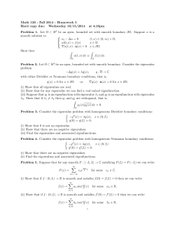


© Copyright 2026