
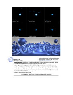
Induction sounding of the Earth`s mantle at a new Russian
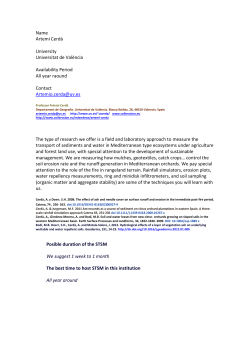
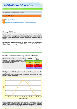
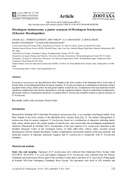
Acta Geophysica
vol. 63, no. 2, Apr. 2015, pp. 385-397
DOI: 10.2478/s11600-014-0245-2
y
Induction Sounding of the Earth’s Mantle
at a New Russian Geophysical Observatory
op
John MOILANEN and Pavel Yu. PUSHKAREV
Lomonosov Moscow State University, Moscow, Russia
e-mails: [email protected], [email protected]
rc
Abstract
A
ut
ho
Deep magnetotelluric (MT) sounding data were collected and processed in the western part of the East European Craton (EEC). The MT
sounding results correspond well with impedances obtained by magnetovariation (MV) sounding on the new geophysical observatory situated
not far from the western border of Russia. Inversion based on combined
data of both induction soundings let us evaluate geoelectrical structure of
the Earth’s crust and upper and mid-mantle at depths up to 2000 km, taking into account the harmonics of 11-year variations. Results obtained by
different authors and methods are compared with similar investigations
on the EEC such as international projects CEMES in Central Europe and
BEAR in Fennoscandia.
Key words: mantle, geoelectrical structure, East European Craton.
1.
INTRODUCTION
By the late 2011, 35 European geomagnetic observatories have been registered in the International Real Time Magnetic Observatory Network
(INTERMAGNET). Only one of these, Borok (58°04′ N, 38°14′ E), is operating in the European part of Russia (Anisimov et al. 2008). It is evident that
the development of geophysical observatories in Russia is important for the
international community to investigate the Earth’s crust and mantle, for ex________________________________________________
Ownership: Institute of Geophysics, Polish Academy of Sciences;
© 2015 Moilanen and Pushkarev. This is an open access article distributed under the Creative
Commons Attribution-NonCommercial-NoDerivs license,
http://creativecommons.org/licenses/by-nc-nd/3.0/.
386
J. MOILANEN and P.YU. PUSHKAREV
2.
rc
op
y
ample, by monitoring the physical fields. The Aleksandrovka Observatory
belongs to the geophysical base of the Moscow University (250 km to the
south-west of Moscow) which has been under construction since 2006. The
place is poorly populated; there are no other settlements within a radius of
8 km and the distance to the nearest DC electrified railway is over 50 km,
thus ensuring a low level of industrial noise. The settlement is electrified and
the base is provided with diesel-generator emergency electric power. Internet
communication is supported by two-way (GPS/GLONASS) satellite systems. The non-magnetic pavilion construction has been completed
(54°53′79′′ N and 35°00′87′′ E) and geophysical data have been collected
since May 2011. The purpose of the Observatory is to measure the full vector of the Earth’s magnetic field (LEMI 025 fluxgate magnetometer; Korepanov et al. 1998), and to carry out uninterrupted recording of variations in
horizontal components of the electric field (Shustov et al. 2012). Seismological three-component measurement stations were also installed. We hope
to install proton magnetometer for absolute values of magnetic field measurement in the nearest future.
THEORETICAL BASE
A
ut
ho
The impedance is the basis of induction soundings. It was introduced by Leontovich in Russia at the beginning of 1930s (Rytov 1940). The strict theory
of radio-waves spreading in the medium was developed by Rytov, who was
Leontovich’s follower (see Senior and Volakis 1995). Induction soundings
were put into practice using equations for the first term of series. They were
obtained for the boundary between isolated and conductive media. The impedance was considered as a scalar, or strictly speaking the functional of
conductivity distribution via skin depth (Rikitake 1948, Tikhonov 1950,
Cagniard 1953). Today, the impedance is a matrix that is formed by anisotropy or heterogeneity of the medium. It was introduced by Berdichevsky and
Cantwell (see Berdichevsky and Dmitriev 2008). Equations for magnetotelluric (MT) and generalized magnetovariation (GMV) soundings are as follows:
E x (ω ) = Z xx (ω ) Bx (ω ) + Z xy (ω ) B y (ω ),
E y (ω ) = Z yx (ω ) Bx (ω ) + Z yy (ω ) B y (ω ),
Bx (ω ) = Yxx (ω ) E x (ω ) + Yxy (ω ) E y (ω ),
(1)
B y (ω ) = Yyx (ω ) E x (ω ) + Yyy (ω ) E y (ω ),
Bz (ω ) ≈ C (ω , r ) div Bτ (ω ) + grad C (ω , r ) Bτ (ω ) .
(1а)
Here C(ω, r) is a response function in GMV sounding method, where r is
a radius vector. It is transformed into apparent resistivity in SI with the for-
INDUCTION STUDY AT THE NEW OBSERVATORY
387
mula: ρ* = iωμ0C2 where i is the imaginary unit, μ0 = 4π10–7 [Henry/m]
the permeability of the free space, ω = 2π/T the circular frequency and
Т-the period. The laconic Eq. 1a was formulated by Guglielmi and Gokhberg (1987), and Schmucker (2003). A more precise theory was presented
by Shuman and Kulik (2002), and Shuman (2007) (see Semenov and
Shuman 2010). The complex Fourier amplitudes for the corresponding
components of MT field, Bτ, Ex, Ey, Bx, By, Bz, are connected through matrices of impedance ||Z|| and admittance ||Y||:
⎛ Yxx
Y =⎜
⎜ Yyx
⎝
Yxy ⎞
⎟.
Yyy ⎟⎠
y
Z xy ⎞
⎟,
Z yy ⎟⎠
(2)
op
⎛ Z xx
Z =⎜
⎜ Z yx
⎝
A
ut
ho
rc
For an isotropic horizontal uniform medium, grad С = 0 (components of
this vector on the x and y axis are different from tippers). The Eq. 1а can be
transformed to the equality Bz(ω) ≈ C(ω, r) div Bτ(ω), which was introduced
for MV soundings by Berdichevsky et al. (1969) and Schmucker (1970). It
can be simplified for Dst variations, because the field induced by ring currents in the magnetosphere is linearly polarized in the Earth (Olsen 1998).
This field is sufficient for defining the Earth response function (Banks
1969):
2 Bθ (ω )
(3)
iω Br (ω ) = C (ω , r )
.
R μ0 tg (θ 0 )
Here R is the Earth’s radius, θ0 the geomagnetic colatitude of observation
place, and Br, Bθ the spectra of radial and colatitude components of the magnetic field. Equation 3 is valid in geomagnetic coordinate system on the
sphere.
If all the elements of impedance matrix are found and Zxx ≡ Zyy = 0,
Zxy = Zyx = Z regardless of the direction (uncommon case in practice), the
conductive medium can be presented as uniform, isotropic halfspace with
one scalar impedance Z(ω). It is transformed to the scalar resistivity as follows
μ Z2
(4)
ρ= 0 .
ω
In a more common case, Zxy ≠ Zyx and additional impedances are nonzero. Then we have a non isotropic medium. In the best case it can be described by tangential anisotropic uniform halfspace. Its resistivity is defined
by plate tensor. Components of apparent resistivity tensor can be found by
the following expressions (Eq. 5), which were obtained theoretically from
Maxwell equations by Reilly (1979) (see Weckmann et al. 2003) and Semenov (2000):
388
J. MOILANEN and P.YU. PUSHKAREV
(
)
) ω,
(
)
) ω.
2
ρ xx = μ0 Z xy
− Z xx Z yy ω , ρ xy = μ0 Z xx Z yx − Z xy ω ,
(
ρ yx = μ0 Z yy Z xy − Z yx
(
2
− Z xx Z yy
ρ yy = μ0 Z yx
(5)
Effective apparent resistivity is used for heterogeneous media. It is usually defined from polar diagrams of impedance or admittance matrixes.
However, you can quite easily localize the heterogeneity place by examining
the effective apparent resistivity. It can be calculated by using the generally
accepted formula, without guidance of possible heterogeneity degree:
y
ρeff = μ0 ( Z xx Z yy − Z xy Z yx ) ω .
(6)
3.
rc
op
This approach is well applicable during anomalous conductivity zones
searching in exploration geophysics. But it is inadmissible during deep
Earth’s research because of the lack of proven data (drilling is well proven
data for exploration geophysics).
Model with horizontal anisotropy is worth to be considered for conductive structure definition of the Earth’s mantle. Its anomalous zones are local.
It can be modeled by stratified, anisotropic structure in regional scale.
DATA PROCESSING
A
ut
ho
Processing of MT data leads to defining the elements of MT matrix (Berdichevsky and Dmitriev 2008), i.e., two unknowns from one of Eqs. 1.
In the GMV sounding case (Eq. 1a) the number of unknowns increases
to three at least: scalar impedance and two tippers. Such a decision can be
evaluated just under the assumption that the number of process realizations
is big enough, for example, in the context of the theory of stochastic processes.
The obtained values have a stochastic character and so are characterized
by confidence intervals under the assumption that displacement errors (bias),
which depend on noises, are small. This is indicated by the corresponding
coherencies (Reddy and Rankin 1974). There is a method to avoid bias by
correlation of all observed data with similar data in a remote point (Gamble
et al. 1979).
There are a lot of algorithms for defining ||Z|| and ||Y|| matrices by records of MT field. For example, one method is based on narrow band digital
filtration (Narsky 1994, Berdichevsky and Dmitriev 2002), another one is
based on classical method of spectral analysis (Sims et al. 1971), and a third
one analyzes data in time domain (Nowożyński 2004). There is an interesting fact. The theory is constructed for a single frequency but impedances often characterize a certain band. It is also a set of realizations but for
neighbouring frequencies.
389
op
y
INDUCTION STUDY AT THE NEW OBSERVATORY
A
ut
ho
rc
Fig. 1. An example of 15-day interval of MT field registered on the Aleksandrovka
Observatory in June 2011. Вx and Вy are the components of magnetic induction vector, x the direction to the geographical north, y to the east, Ex and Ey are the components of electric field; the length of receiving lines is 100 m.
Fig. 2. Removing diurnal variations on the example of 15-days record on Alexandrovka base in June 2011 (Bx – component of the magnetic field, BxSq – filtration
result).
The MT data chosen for analysis were obtained in summer 2011. Some
part of these data is presented in Fig. 1. While defining impedances it is necessary to switch from Eq. 1 for monochromatic electromagnetic wave to
a continuous distribution of spectral frequency. Spectral distributions of field
390
J. MOILANEN and P.YU. PUSHKAREV
A
ut
ho
rc
op
y
components let the required functions values with their casual errors and bias
(it is often higher than casual errors). The coherence defines reliability of
implementation of Eqs. 1, 1а for real data (Semenov 2000).
For a long period, the data processing was performed by using the Petrischev/Tkachev program (Method 1, Semenov 1985). Processing scheme of
MT-data in this method includes removing short-term spikes with a nonlinear filter (Naudy and Dreyer 1968), removing diurnal harmonics of observed
field (Fig. 2) (Parkinson 1983) and, finally, selection of data with high coherency, i.e., less distorted sections with noises.
It is worth noting that the main directions for different periods are different. Three sections were selected. The main direction was selected to be 150
degrees for the first section, T ∈ [30, 2500] s; 170 degrees for the second
section, T ∈ [2500, 8000] s; and 150 degrees (the same as at the first one) for
the third section, T ∈ [8000, 25 000] s (Fig. 3). The second processing stage
includes analyzing the whole record with the selected main direction. Different displacement windows are chosen. This window is charged with the
length of data for the fast Fourier transform.
Fig. 3. Polar diagrams of primary and additional components of apparent resistivity
2
, Co 2yx –
tensor [Ohm·m] (upper image) and square coherencies: Co2pl – plural, Coxy
2
singular, Coxx – input signals (bottom), received for impedance Z (left) and admittance Y (right) estimations for T = 10 000 s.
INDUCTION STUDY AT THE NEW OBSERVATORY
391
A
ut
ho
rc
op
y
The observed data were processed by different algorithms. The first
method was used for processing just on the Aleksandrovka Observatory.
Varentsov’s algorithm (Method 2) was used in multi reference scheme. It is
formed on robust averaging of estimates for several base points. Also, there
were some boundary conditions on horizontal MV response changes between investigation point and remote bases (Varentsov 2007).
Additional MT and Audio-MT three-day’s data were added to the joint
process by Varentsov’s and Larsen’s algorithms (Larsen et al. 1996)
(Method 3).
Fig. 4. Complex apparent resistivities of central part of the EEC estimated by three
independent MT routines at the Aleksandrovka Observatory and GMV method at the
Moscow Observatory.
392
4.
J. MOILANEN and P.YU. PUSHKAREV
COMPARISON OF PROCESSING RESULTS
THE INVERSION
A
ut
ho
5.
rc
op
y
Method 1 does not take into account frequency characteristics of the equipment. Results obtained by this algorithm differ from the Varentsov’s and
Larsen’s algorithms in low period area (Fig. 4). It is necessary to consider
frequency characteristics of the equipment for the period range lower than
600 s (T < 6000 s). Reliability of acquired data was improved using several
base stations and robust averaging procedure. This is well seen especially in
the long period area (T > 6000 s). The results of different processing are well
corresponding up to the period of T ≈ 3 hours (T = 104 s). Then serious discrepancies occur (Semenov and Shuman 2010, Shimizu et al. 2011). Three
kinds of source fields are dominant at the period range 104-105 s daily oscillations (Sq variations) connected with the Earth’s rotation, bays caused by
polar cusp currents, and Dst variations caused by the magnetospheric ring
current. The bays can be considered as a plane wave (Vanyan et al. 2002)
with the vertical magnetic component in the middle latitudes, while the Dst
variations contain the stable magnetic field which is collinear with geomagnetic axis (Banks 1981, Fujii and Shultz 2002). However, the MT soundings
can be replaced by GMV soundings for the periods of 3-30 hours (Semenov
et al. 2011). The data of Moscow Observatory (CEMES project, Semenov et
al. 2008) were used for those purposes (Fig. 4).
First of all, the phase inversion of the impedance was accomplished by
OCCAM algorithm (Constable et al. 1987). Thus, the module of apparent resistivity tensor was corrected for surface heterogeneity obtained by MT data
(Fig. 5).
Inversions by the well-known OCCAM and D+ algorithms were held for
corrected responses of MT and GMV methods. D+ let us create geoelectrical
horizontal layered media. Conductive layers approximate by thin layers with
finite conductance (Parker 1980).
Sediments, crust, asthenosphere, and mid-mantle layer were picked out
during 1D interpretation (Fig. 6a). The sediments of Moscow syncline have a
thickness of 800 m.
The upper boundary of asthenosphere was picked out at a depth of
280 km. The upper boundary of the mid-mantle layer is at a depth of
660 km. The D+ results are quite representative. The upper boundary of the
asthenosphere has a depth of 230 km. The mid-mantle layer has its edges at
depths of 670 and 900 km. Additional conductive layer was picked out by
the D+ algorithm. It has the conductance of 160 S at a depth of 65 km. We
think this layer can be the appearance of the conductive layers of the lower
crust. They should be shallower. We used previous investigations for evalua-
393
op
y
INDUCTION STUDY AT THE NEW OBSERVATORY
rc
Fig. 5. The correction result obtained by OCCAM (dashed black) algorithm. Complex apparent resistivities estimated by the MT method for Aleksandrovka are
shown as empty points and the MV method for the Moscow Observatory are shown
as error bars.
(b)
A
ut
ho
(a)
Fig. 6. Comparison of inversion results of MT and MV data for Aleksandrovka and
Moscow Observatories; solid line is the OCCAM decision, arrows show D+ thin
layers with their conductance (left panel) and conductance comparison obtained on
different observatories. ALX – Aleksandrovka Observatory, BEAR – Fennoscandian
experiment (Varentsov et al. 2002, Sokolova and Varentsov 2007), BEL – observatory in Poland, LOW – observatory in Sweden. Data from two last observatories
were obtained during CEMES project (Semenov and Jozwiak 2006, Semenov et
al. 2008).
tion of the obtained results. These were the BEAR project, based on data obtained in Fennoscandian region, and CEMES in the central part of Europe.
394
J. MOILANEN and P.YU. PUSHKAREV
The comparison was carried out by the curves of integral conductance
(Fig. 6b). The choice was made of the S curves. Each conductivity distribution corresponds with the one conductance value. So the uniqueness theorem
for 1D inversion is proved only for infinite frequency range.
6.
RESULTS AND DISCUSSION
rc
op
y
Aleksandrovka is a geophysical observatory of Moscow University. Longperiod registration of MT-field is held here. The obtained data were processed by several authors with different algorithms, such as the only observation point processing or using several base stations. The robust estimation
was used. It has become a standard procedure during MT data processing.
We have got close results for T < 104 s for all researching algorithms.
For longer periods it is hard to get truthful estimations due to several reasons. Estimation procedures of transfer operators for several base stations
improve processing result. The obtained results correspond well with deep
geoelectrical mantle properties. Moreover, they figure on a relative homogeneity of the mantle on the EEC. The sharp increase of mantle conductivity
begins with depths of 300-400 km. We think it is connected with the asthenosphere.
A
ut
ho
A c k n o w l e d g m e n t s . The authors express appreciation to I. Varentsov, N. Palshin for processed MT materials, M. Petrishchev, A. Tkachev,
and J. Larsen for vested algorithms. The authors also acknowledge to the reviewers, V.Yu. Semenov and anonymous one, for their valuable remarks.
References
Anisimov, S.V., E.M. Dmitriev, N.K. Sycheva, A.N. Sychev, V.P. Shcherbakov, and
Y.K. Vinogradov (2008), Information technology in geomagnetic measurements perfomed in the Borok Geophysical Observatory, Geofiz. Icc. 9,
3, 62-76 (in Russian).
Banks, R.J. (1969), Geomagnetic variations and the electrical conductivity of the
upper mantle, Geophys. J. Int. 17, 5, 457-487, DOI: 10.1111/j.1365-246X.
1969.tb00252.x.
Banks, R.J. (1981), Strategies for improved global electromagnetic response estimates, J. Geomagn. Geoelectr. 33, 11, 569-585, DOI: 10.5636/jgg.33.569.
Berdichevsky, M.N., and V.I. Dmitriev (2002), Magnetotellurics in the Context of
the Theory of Ill-Posed Problems, Investigations in Geophysics, No. 11,
Society of Exploration Geophysicists, Tulsa, 215 pp.
INDUCTION STUDY AT THE NEW OBSERVATORY
395
Berdichevsky, M.N.,and V.I. Dmitriev (2008), Models and Methods of Magnetotellurics, Springer, Berlin, 563 pp.
Berdichevsky, M.N., L.L. Vanyan, and E.B. Fainberg (1969), The frequency sounding of the Earth by spherical analysis of electromagnetic variations, Geomagn. Aeronomy 9, 2, 372-374 (in Russian).
Cagniard, L. (1953), Basic theory of the magneto-telluric method of geophysical
prospecting, Geophysics 18, 3, 605-635, DOI: 10.1190/1.1437915.
y
Constable, S.C., R.L. Parker, and C.G. Constable (1987), Occam’s inversion:
A practical algorithm for generating smooth models from electromagnetic
sounding data, Geophysics 52, 3, 289-300, DOI: 10.1190/1.1442303.
op
Fujii, I., and A. Schultz (2002), The 3D electromagnetic response of the Earth to
ring current and auroral oval excitation, Geophys. J. Int. 151, 3, 689-709,
DOI: 10.1046/j.1365-246X.2002.01775.x.
Gamble, T.D., W.M. Goubau, and J. Clarke (1979), Magnetotellurics with a remote
magnetic reference, Geophysics 44, 1, 53-68, DOI: 10.1190/1.1440923.
rc
Guglielmi, A.V., and M.B. Gokhberg (1987), On the magnetotelluric sounding in
the seismically active areas, Izv. – Phys. Solid Earth 33, 11, 122-123 (in
Russian).
A
ut
ho
Korepanov, V., A. Best, B. Bondaruk, H.-J. Linthe, J. Marianiuk, K. Pajunpää,
L. Rakhlin, and J. Reda (1998), Experience of observatory practice with
LEMI-004 magnetometers, Rev. Geofis. 48, 31-40.
Larsen, J.C., R.L. Mackie, A. Manzella, A. Fiordelisi, and S. Rieven (1996), Robust
smooth magnetotelluric transfer functions, Geophys. J. Int. 124, 3, 801-819,
DOI: 10.1111/j.1365-246X.1996.tb05639.x.
Narsky, N.V. (1994), Robust methods of processing magnetotelluric variation, Ph.D.
Thesis, Moscow State University, Moscow, Russia, 130 pp. (in Russian).
Naudy, H., and H. Dreyer (1968), Essai de filtrage non-linéaire appliqué aux profils
aéromagnétiques, Geophys. Prospect. 16, 2, 171-178, DOI: 10.1111/j.13652478.1968.tb01969.x (in French).
Nowożyński, K. (2004), Estimation of magnetotelluric transfer functions in the time
domain over a wide frequency band, Geophys. J. Int. 158, 1, 32-41, DOI:
10.1111/j.1365-246X.2004.02288.x.
Olsen, N. (1998), The electrical conductivity of the mantle beneath Europe derived
from C-responses from 3 to 720 hr, Geophys. J. Int. 133, 2, 298-308, DOI:
10.1046/j.1365-246X.1998.00503.x.
Parker, R.L. (1980), The inverse problem of electromagnetic induction: Existence
and construction of solutions based on incomplete data, J. Geophys. Res.
85, B8, 4421-4428, DOI: 10.1029/JB085iB08p04421.
Parkinson, W.D. (1983), Introduction to Geomagnetism, Scottish Academic Press,
Edinburgh, 433 pp.
396
J. MOILANEN and P.YU. PUSHKAREV
Reddy, I.K., and D. Rankin (1974), Coherence functions for magnetotelluric analysis, Geophysics 39, 3, 312-320, DOI: 10.1190/1.1440430.
Reilly, W.I. (1979), Anisotropy tensors in magnetotelluric application, Tech. Rep.,
Department of Scientific and Industrial Research, Wellington, New Zealand.
Rikitake, T. (1948), Notes on electromagnetic induction within the Earth, Bull.
Earthq. Res. Inst. 24, 1/4, 1-9.
y
Rytov, S.E. (1940), Calculation of the skin-effect by the perturbation method,
J. Exp. Theor. Phys. 10, 2, 180-189 (in Russian).
op
Schmucker, U. (1970), Anomalies of Geomagnetic Variations in the Southwestern
United States, University of California Press, Berkeley.
Schmucker, U. (2003), Horizontal spatial gradient sounding and geomagnetic depth
sounding in the period range of daily variations. In: A. Hördt and J.B. Stoll
(eds.), Protokoll über das Kolloquium Elektromagnetische Tiefenforschung,
29.09.-3.10.2003, Königstein, Deutschland, 306-317.
rc
Semenov, V.Yu. (1985), Processing of Magnetotelluric Sounding Data, Nedra,
Moscow, 133 pp. (in Russian).
Semenov, V.Yu. (2000), On the apparent resistivity in magnetotelluric sounding,
Izv. – Phys. Solid Earth 36, 1, 99-100.
A
ut
ho
Semenov, V.Yu., and W. Jozwiak (2006), Lateral variations of the mid-mantle conductance beneath Europe, Tectonophysics 416, 1-4, 279-288, DOI: 10.1016/
j.tecto.2005.11.017.
Semenov, V.Yu., and V.N. Shuman (2010), Impedances for induction soundings of
the Earth’s mantle, Acta Geophys. 58, 4, 527-542, DOI: 10.2478/s11600010-0003-z.
Semenov, V.Yu., J. Pek, A. Ádám, W. Jóźwiak, B. Ladanyvskyy, I.M. Logvinov,
P. Pushkarev, and J. Vozar (2008), Electrical structure of the upper mantle
beneath Central Europe: Results of the CEMES project, Acta Geophys. 56,
4, 957-981, DOI: 10.2478/s11600-008-0058-2.
Semenov, V.Yu., B. Ladanivskyy, and K. Nowożyński (2011), New induction
sounding tested in central Europe, Acta Geophys. 59, 5, 815-832, DOI:
10.2478/s11600-011-0030-4.
Senior, T.B., and J.L. Volakis (1995), Approximate Boundary Conditions in Electromagnetics, IEE Press, London, 353 pp.
Shimizu, H., A. Yoneda, K. Baba, H. Utada, and N.A. Palshin (2011), Sq effect on
the electromagnetic response functions in the period range between 104 and
105 s, Geophys. J. Int. 186, 1, 193-206, DOI: 10.1111/j.1365-246X.2011.
05036.x.
Shuman, V.N. (2007), Imaginary surface vectors in multidimensional inverse problems of geoelectrics, Izv. – Phys. Solid Earth 43, 3, 205-210, DOI: 10.1134/
S1069351307030044.
INDUCTION STUDY AT THE NEW OBSERVATORY
397
Shuman, V., and S. Kulik (2002), The fundamental relations of impedance type in
general theories of the electromagnetic induction studies, Acta Geophys.
Pol. 50, 4, 607-618.
y
Shustov, N.L., V.A. Kulikov, E.V. Moilanen, A.Yu. Polenov, P.Yu. Pushkarev,
V.K. Khmelevskoi, and A.G. Yakovlev (2012), The creation of a geophysical observatory at the Aleksandrovka research base of the Geological Faculty of Moscow State University in the Kaluga Region, Moscow Univ.
Geol. Bull. 67, 4, 253-258, DOI: 10.3103/S0145875212040096.
Sims, W.E., F.X. Bostick, and H.W. Smith (1971), The estimation of magnetotelluric impedance tensor elements from measured data, Geophysics 36, 5, 938942, DOI: 10.1190/1.1440225.
op
Sokolova, E.Yu., and I.M. Varentsov (2007), Deep array electromagnetic sounding
on the Baltic Shield: External excitation model and implications for upper
mantle conductivity studies, Tectonophysics 445, 1-2, 3-25, DOI: 10.1016/
j.tecto.2007.07.006.
rc
Tikhonov, A.N. (1950), On determining electrical characteristics of the deep layers
of the Earth’s crust, Doklady 73, 2, 295-297.
Vanyan, L.L., V.A. Kuznetsov, T.V. Lyubetskaya, N.A. Palshin, T. Korja, I. Lahti,
and BEAR Working Group (2002), Electrical conductivity of the crust beneath Central Lapland, Izv. – Phys. Solid Earth 38, 10, 798-815.
A
ut
ho
Varentsov, I.M. (2007), Arrays of simultaneous electromagnetic soundings: design,
data processing and analysis. In: V.V. Spichak (ed.), Electromagnetic
Sounding of the Earth’s Interior, Methods in Geochemistry and Geophysics, Vol. 40, Elsevier, Amsterdam, 259-275.
Varentsov, I.M., M. Engels, T. Korja, M.Yu. Smirnov, and the BEAR Working
Group (2002), A generalised geoelectric model of Fennoscandia: A challenging database for long-period 3D modelling studies within the Baltic
Electromagnetic Array Research (BEAR) Project, Izv. – Phys. Solid Earth
38, 11, 855-896.
Vozar, J., and V.Yu. Semenov (2010), Compatibility of induction methods for mantle soundings, J. Geophys. Res. 115, B3, B03101, DOI: 10.1029/2009JB
006390.
Weckmann, U., O. Ritter, and V. Haak (2003), Images of the magnetotelluric apparent resistivity tensor, Geophys. J. Int. 155, 2, 456-468, DOI: 10.1046/
j.1365-246X.2003.02062.x.
Received 22 November 2013
Received in revised form 27 March 2014
Accepted 7 April 2014


© Copyright 2026