
IMPACTS of Impervious Cover on Aquatic Systems
Watershed Protection Research Monograph No. 1
IMPACTS
of Impervious
Cover on
Aquatic Systems
Center for
Watershed
Protection
March 2003
Cover photograph Ellicott City, Maryland 2003.
Courtesy Anne Kitchell, Center for Watershed Protection.
Watershed Protection Research Monograph No. 1
Impacts of Impervious
Cover on Aquatic Systems
March 2003
Prepared by:
Center for Watershed Protection
8391 Main Street
Ellicott City, MD 21043
www.cwp.org
www.stormwatercenter.net
Copyright (c) 2003 by the Center for Watershed Protection.
Material may be quoted provided credit is given. Printed in the
United States of Amercia on recycled paper.
Foreword
Foreword
We are extremely pleased to launch the first
edition of a new series called Watershed
Protection Research Monographs. Each
monograph will synthesize emerging research
within a major topical area in the practice of
watershed protection. The series of periodic
monographs will replace our journal
Watershed Protection Techniques, which
lapsed in 2002. We hope this new format will
provide watershed managers with the science
and perspectives they need to better protect and
restore their local watersheds.
This monograph was written to respond to
many inquiries from watershed managers and
policy makers seeking to understand the
scientific basis behind the relationship between
impervious cover and the health of aquatic
ecosystems. It reviews more than 225 research
studies that have explored the impact of
impervious cover and other indicators of
urbanization on aquatic systems. This report
comprehensively reviews the available scientific data on how urbanization influences
hydrologic, physical, water quality, and
biological indicators of aquatic health, as of
late 2002.
Our intention was to organize the available
scientific data in a manner that was accessible
to watershed leaders, policy-makers and
agency staff. In addition, the research itself,
which spans dozens of different academic
departments and disciplines, was conducted in
many different eco-regions, climatic zones,
and stream types. In order to communicate
across such a wide audience, we have resorted
to some simplifications, avoided some important particulars, refrained from some jargon,
and tried, wherever possible, to use consistent
terminology. Thus, the interpretations and
conclusions contained in this document are
ours alone, and our readers are encouraged to
consult the original sources when in doubt.
We would also like to note that the Center for
Watershed Protection and the University of
Alabama are currently developing a major
national database on stormwater quality. The
database will contain nearly 4,000 stationstorm events collected by municipalities as part
of the U.S. EPA’s National Pollutant Discharge
Elimination System (NPDES) Phase I Stormwater Permit Program. We anticipate releasing
a data report in late 2003 that will provide a
much needed update of stormwater event mean
concentrations (EMCs).
As of this writing, many research efforts are
underway that will further test and refine these
relationships (most notably, the U.S. Geological Survey gradients initiative, but also many
other local, state and academic efforts). We
hope that this report provides a useful summary of the existing science, suggests some
directions for new research, and stimulates
greater discussion of this important topic in
watershed management. We also feel it is time
for a major conference or symposium, where
this diverse community can join together to
discuss methods, findings and the important
policy implications of their research.
Impacts of Impervious Cover on Aquatic Systems
i
Foreword
ii
Impacts of Impervious Cover on Aquatic Systems
Acknowledgments
Acknowledgments
Putting this first research monograph together took a lot of energy, editing and analysis, and
many Center staff devoted their time and energy over the last two years to get it done. The
project team consisted of Karen Cappiella, Deb Caraco, Samantha Corbin, Heather Holland,
Anne Kitchell, Stephanie Linebaugh, Paul Sturm, and Chris Swann. Special thanks are extended
to Tiffany Wright, who worked tirelessly to assemble, edit and otherwise polish the final draft.
I am also grateful to Michael Paul of Tetratech, Inc., who graciously provided us with an extensive literature review from his PhD days at the University of Georgia that contained many
obscure and hard to find citations. Portions of this monograph were developed as part of a
literature review conducted as part of a work assignment for the U.S. EPA Office of Wastewater
Management in 2001, which proved indispensable in our efforts. Lastly, I would like to thank the
hundreds of scientists who have contributed their time and data to explore and test the relationships between urbanization and aquatic health.
Tom Schueler
Center for Watershed Protection
Impacts of Impervious Cover on Aquatic Systems
iii
Acknowledgments
iv
Impacts of Impervious Cover on Aquatic Systems
Table of Contents
Table of Contents
Foreword
..................................................................................................................................... i
Acknowledgments .................................................................................................................................... iii
List of Acronyms and Abbreviations ........................................................................................................... xi
Chapter 1: Introduction
1.1 Is Impervious Cover Still Important? A Review of Recent Stream Research ............................ 1
1.1.1
Strength of the Evidence for the ICM ..................................................................... 3
1.1.2
Reinterpretation of the ICM ..................................................................................... 5
1.1.3
Influence of Watershed Treatment Practices on the ICM ................................... 9
1.1.4
Recommendations for Further ICM Research ..................................................... 12
1.2 Impacts of Urbanization on Downstream Receiving Waters .................................................... 14
1.2.1
Relationship Between Impervious Cover and Stormwater Quality ................... 14
1.2.2
Water Quality Response to Stormwater Pollution ................................................ 15
1.2.3
Effect of Watershed Treatment on Stormwater Quality ..................................... 18
1.3 Implications of the ICM for Watershed Managers .................................................................... 21
1.3.1
Management of Non-Supporting Streams............................................................ 21
1.3.2
Use of the ICM for Urban Stream Classification .................................................. 22
1.3.3
Role of the ICM In Small Watershed Planning ..................................................... 22
1.4 Summary
.................................................................................................................................. 24
Chapter 2: Hydrologic Impacts of Impervious Cover
2.1 Introduction .................................................................................................................................. 25
2.2 Increased Runoff Volume ............................................................................................................. 27
2.3 Increased Peak Discharge Rate .................................................................................................. 30
2.4 Increased Bankfull Flow ................................................................................................................ 31
2.5 Decreased Baseflow ..................................................................................................................... 34
2.6 Conclusions .................................................................................................................................. 37
Chapter 3: Physical Impacts of Impervious Cover
3.1 Difficulty in Measuring Habitat ..................................................................................................... 40
3.1.1
The Habitat Problem ............................................................................................... 40
3.2 Changes in Stream Geometry ..................................................................................................... 42
3.2.1
Channel Enlargement ............................................................................................ 42
3.2.2
Effect of Channel Enlargement on Sediment Yield ............................................ 45
3.3 Effect on Composite Measures of Stream Habitat .................................................................... 46
3.4 Effect on Individual Elements of Stream Habitat ....................................................................... 47
3.4.1
Bank Erosion and Bank Stability ............................................................................. 47
3.4.2
Embeddedness ....................................................................................................... 47
3.4.3
Large Woody Debris (LWD) .................................................................................... 49
3.4.4
Changes in Other Individual Stream Parameters ............................................... 49
3.5 Increased Stream Warming ......................................................................................................... 50
3.6 Alteration of Stream Channel Networks ..................................................................................... 52
3.6.1
Channel Modification ............................................................................................ 52
3.6.2
Barriers to Fish Migration ......................................................................................... 53
3.7 Conclusion .................................................................................................................................. 54
Chapter 4: Water Quality Impacts of Impervious Cover
4.1 Introduction .................................................................................................................................. 55
4.2 Summary of National and Regional Stormwater Pollutant Concentration Data .................. 56
4.2.1
National Data .......................................................................................................... 56
4.2.2
Regional Differences Due to Rainfall ................................................................... 56
4.2.3
Cold Region Snowmelt Data ................................................................................. 58
4.3 Relationship Between Pollutant Loads and Impervious Cover: The Simple Method ............. 61
4.4 Sediment
.................................................................................................................................. 63
Impacts of Impervious Cover on Aquatic Systems
v
Table of Contents
4.4.1
Concentrations ....................................................................................................... 63
4.4.2
Impacts of Sediment on Streams .......................................................................... 63
4.4.3
Sources and Source Areas of Sediment .............................................................. 64
4.5 Nutrients
.................................................................................................................................. 67
4.5.1
Concentrations ....................................................................................................... 67
4.5.2
Impacts of Nutrients on Streams ........................................................................... 68
4.5.3
Sources and Source Areas of Nutrients ................................................................ 69
4.6 Trace Metals .................................................................................................................................. 71
4.6.1
Concentrations ....................................................................................................... 71
4.6.2
Impacts of Metals on Streams ............................................................................... 72
4.6.3
Sources and Source Areas of Trace Metals ......................................................... 73
4.7 Hydrocarbons: PAH, Oil and Grease ......................................................................................... 75
4.7.1
Concentrations ....................................................................................................... 75
4.7.2
Impacts of Hydrocarbons on Streams .................................................................. 75
4.7.3
Sources and Source Areas of Hydrocarbons ...................................................... 76
4.8 Bacteria & Pathogens .................................................................................................................. 77
4.8.1
Concentrations ....................................................................................................... 77
4.8.2
Impacts of Bacteria and Pathogens on Streams ................................................ 79
4.8.3
Sources and Source Areas of Bacteria and Pathogens .................................... 80
4.9 Organic Carbon ............................................................................................................................ 82
4.9.1
Concentrations ....................................................................................................... 82
4.9.2
Impacts of Organic Carbon on Streams .............................................................. 82
4.9.3
Sources and Source Areas of Total Organic Carbon ......................................... 82
4.10
MTBE
.................................................................................................................................. 83
4.10.1 Concentrations ....................................................................................................... 83
4.10.2 Impacts of MTBE on Streams .................................................................................. 83
4.10.3 Sources and Source Areas of MTBE ...................................................................... 84
4.11
Pesticides ............................................................................................................................... 85
4.11.1 Concentrations ....................................................................................................... 86
4.11.2 Impacts of Pesticides on Streams ......................................................................... 86
4.11.3 Sources and Source Areas of Pesticides .............................................................. 87
4.12
Deicers .................................................................................................................................. 88
4.12.1 Concentrations ....................................................................................................... 89
4.12.2 Impacts of Deicers on Streams ............................................................................. 89
4.12.3 Sources and Source Areas of Deicers .................................................................. 90
4.13
Conclusion ............................................................................................................................. 91
Chapter 5: Biological Impacts of Impervious Cover
5.1 Introduction .................................................................................................................................. 93
5.2 Indicators and General Trends .................................................................................................... 95
5.2.1 Biological Indicators ................................................................................................. 95
5.2.2 Watershed Development Indices .......................................................................... 95
5.2.3 General Trends ......................................................................................................... 97
5.3 Effects on Aquatic Insect Diversity ............................................................................................ 100
5.3.1 Findings Based on Impervious Cover Indicators .................................................. 100
5.3.2 Findings Based on Other Development Indicators ............................................. 104
5.4 Effects on Fish Diversity ............................................................................................................... 105
5.4.1 Findings Based on Impervious Cover Indicators .................................................. 105
5.4.2 Findings Based on other Development Indicators .............................................. 110
5.5 Effects on Amphibian Diversity .................................................................................................. 112
5.6 Effects on Wetland Diversity ....................................................................................................... 114
5.7 Effects on Freshwater Mussel Diversity ...................................................................................... 115
5.8 Conclusion ................................................................................................................................ 116
References
Glossary
vi
................................................................................................................................ 117
................................................................................................................................ 137
Impacts of Impervious Cover on Aquatic Systems
Table of Contents
List of Tables
1
2
3
4
5
6
7
8
9
10
11
12
13
14
15
16
17
18
19
20
21
22
23
24
25
26
27
28
29
30
31
32
33
34
35
36
37
38
39
40
41
42
43
44
45
The Strength of Evidence: A Review of Current Research on Urban Stream
Quality Indicators ............................................................................................................................. 4
Land Use/IC Relationships for Suburban Areas of the Chesapeake Bay .................................. 9
Summary of Urban Stormwater Pollutant Loads on Quality of Receiving Waters ................... 14
The Effectiveness of Stormwater Treatment Practices in Removing
Pollutants - Percent Removal Rate ............................................................................................... 18
Median Effluent Concentrations from Stormwater Treatment Practices ................................. 19
Additional Considerations for Urban Stream Classification ....................................................... 23
Research Review of Increased Runoff Volume and Peak Discharge in Urban Streams ........ 28
Hydrologic Differences Between a Parking Lot and a Meadow .............................................. 29
Comparison of Bulk Density for Undisturbed Soils and Common Urban Conditions ............... 29
Research Review of Increased Bankfull Discharge in Urban Streams ...................................... 32
Research Review of Decreased Baseflow in Urban Streams .................................................... 34
Physical Impacts of Urbanization on Streams ............................................................................. 41
Research Review of Channel Enlargement and Sediment Transport in Urban Streams ........ 43
Research Review of Changes in Urban Stream Habitat ............................................................ 48
Research Review of Thermal Impacts in Urban Streams ........................................................... 50
National EMCs for Stormwater Pollutants .................................................................................... 57
Regional Groupings by Annual Rainfall Amount ........................................................................ 58
Stormwater Pollutant EMCs for Different U.S. Regions ................................................................ 59
Mean and Median Nutrient and Sediment Stormwater Concentrations for
Residential Land Use Based on Rainfall Regions ......................................................................... 59
EPA 1986 Water Quality Standards and Percentage of Metal Concentrations
Exceeding Water Quality Standards by Rainfall Region ............................................................ 60
Runoff and Pollutant Characteristics of Snowmelt Stages ........................................................ 60
EMCs for Total Suspended Solids and Turbidity ........................................................................... 63
Summary of Impacts of Suspended Sediment on the Aquatic Environment .......................... 64
Summary of Impacts of Deposited Sediments on the Aquatic Environment .......................... 64
Sources and Loading of Suspended Solids Sediment in Urban Areas ...................................... 65
Source Area Geometric Mean Concentrations for Suspended Solids in Urban Areas .......... 66
Mean TSS Inflow and Outflow at Uncontrolled, Controlled and Model Construction Sites ... 66
EMCs of Phosphorus and Nitrogen Urban Stormwater Pollutants ............................................. 67
Source Area Monitoring Data for Total Nitrogen and Total Phosphorus in Urban Areas ........ 69
EMCs and Detection Frequency for Metals in Urban Stormwater ............................................ 71
Average Total Recoverable and Dissolved Metals for 13 Stormwater Flows and
Nine Baseflow Samples from Lincoln Creek in 1994 ................................................................... 72
Percentage of In-situ Flow-through Toxicity Tests Using Daphnia magna and
Pimephales promelas with Significant Toxic Effects from Lincoln Creek .................................. 73
Metal Sources and Source Area “Hotspots” in Urban Areas ..................................................... 74
Metal Source Area Concentrations in the Urban Landscape .................................................. 74
Hydrocarbon EMCs in Urban Areas .............................................................................................. 75
Bacteria EMCs in Urban Areas ...................................................................................................... 78
Cryptosporidium and Giardia EMCs ............................................................................................ 79
Percent Detection of Giardia cysts and Cryptosporidium oocysts in Subwatersheds and
Wastewater Treatment Plant Effluent in the New York City Water Supply Watersheds .......... 80
Typical Coliform Standards for Different Water Uses .................................................................. 80
EMCs for Organic Carbon in Urban Areas .................................................................................. 82
MTBE Detection Frequency ........................................................................................................... 83
Median Concentrations and Detection Frequency of Herbicides and
Insecticides in Urban Streams ....................................................................................................... 85
Use and Water Quality Effect of Snowmelt Deicers ................................................................... 88
EMCs for Chloride in Snowmelt and Stormwater Runoff in Urban Areas ................................. 89
Summary of State Standards for Salinity of Receiving Waters ................................................... 90
Impacts of Impervious Cover on Aquatic Systems
vii
Table of Contents
46
47
48
49
50
51
52
53
54
Review of Stressors to Urban Streams and Effects on Aquatic Life ........................................... 94
Examples of Biodiversity Metrics Used to Assess Aquatic Communities ................................... 96
Alternate Land Use Indicators and Significant Impact Levels .................................................. 98
Recent Research Examining the Relationship Between IC and Aquatic
Insect Diversity in Streams ............................................................................................................ 101
Recent Research Examining the Relationship of Other Indices of Watershed
Development on Aquatic Insect Diversity in Streams .............................................................. 102
Recent Research Examining the Relationship Between Watershed IC
and the Fish Community .............................................................................................................. 106
Recent Research Examining Urbanization and Freshwater Fish Community Indicators ...... 108
Recent Research on the Relationship Between Percent Watershed
Urbanization and the Amphibian Community .......................................................................... 113
Recent Research Examining the Relationship Between Watershed Development
and Urban Wetlands .................................................................................................................... 114
List of Figures
1
2
3
4
5
6
7
8
9
10
11
12
13
14
15
16
17
18
19
20
21
22
23
24
25
26
27
28
29
30
31
32
33
34
35
viii
Impervious Cover Model ................................................................................................................. 2
Typical Scatter Found in IC/Stream Quality Indicator Research ................................................ 5
Relationship of IC and FC in Puget Sound Subwatersheds ......................................................... 6
The Double Scatter Problem: Difficulties in Detecting the Effect of Watershed Treatment .. 10
Estimated Phosphorous Load as a Function of IC, Discounted Stormwater
Treatment and Better Site Design ................................................................................................. 19
Altered Hydrograph in Response to Urbanization ...................................................................... 25
Runoff Coefficient vs. IC ................................................................................................................ 27
Discharge for Urban and Rural Streams in North Carolina ........................................................ 30
Effect on Flood Magnitudes of 30% Basin IC ............................................................................... 31
Relationship of Urban/Rural 100-year Peak Flow Ratio to Basin
Development Factor and IC ......................................................................................................... 31
Increase in Bankfull Flows Due to Urbanization ........................................................................... 32
Increase in Number of Exceedences of Bankfull Flow Over Time With Urbanization ............. 33
Percent of Gage Reading Above Mean Annual Flow .............................................................. 33
Relationship Between Baseflow and Watershed Impervious Cover ........................................ 34
Baseflow Response to Urbanization ............................................................................................. 35
Relationship Between Percentage Baseflow and Percent IC .................................................. 35
Effect of IC on Summer Baseflow (Corrected for Catchment Area) ....................................... 36
Effect of Watershed IC on Summer Stream Velocity .................................................................. 36
Urban Stream Channels with Progressively Greater IC .............................................................. 40
Increased Shear Stress from a Hydrograph ................................................................................. 42
Stream Channel Enlargement in Watts Branch .......................................................................... 44
Ultimate Channel Enlargement .................................................................................................... 45
Relationship Between Habitat Quality and IC in Maine Streams .............................................. 46
Fine Material Sediment Deposition as a Function of IC ............................................................. 47
LWD as a Function of IC ................................................................................................................. 49
Stream Temperature Increase in Response to Urbanization ..................................................... 51
Drainage Network of Rock Creek, D.C. and Four Mile Creek, VA
Before and After Urbanization ...................................................................................................... 52
Fish Migration Barriers in the Urbanized Anacostia Watershed ................................................. 53
Snowmelt Runoff Hydrograph ....................................................................................................... 60
The Simple Method - Basic Equations .......................................................................................... 61
TSS from Bank Erosion vs. IC ........................................................................................................... 65
Nitrate-Nitrogen Concentration in Stormwater Runoff .............................................................. 68
Total Phosphorus Concentration in Stormwater ......................................................................... 68
Total Phosphorus From Bank Erosion as a Function of IC ........................................................... 70
Fecal Coliform Levels in Urban Stormwater ................................................................................ 77
Impacts of Impervious Cover on Aquatic Systems
Table of Contents
36
37
38
39
40
41
42
43
44
45
46
47
48
49
50
51
52
Relationship Between IC and Fecal Coliform Concentrations ................................................. 79
MTBE Concentrations in Surface Water from Eight Cities .......................................................... 83
Concentrations of Pesticides in Stormwater in King County, WA ............................................. 87
U.S. Highway Salt Usage Data ....................................................................................................... 88
Combined Fish and Benthic IBI vs. IC ........................................................................................... 98
Relationship Between B-IBI, Coho/Cutthroat Ratios, and Watershed IC ................................. 99
Index for Biological Integrity as a Function of Population Density ............................................ 99
Trend Line Indicating Decline in Benthic IBI as IC Increases .................................................... 103
Compilation of Puget Lowland Watershed Biological Data ................................................... 103
IC and IBI at Stream Sites in the Patapsco River Basin, MD ..................................................... 103
IC vs. Aquatic Insect Sensitivity - EPT scores in Delaware Streams .......................................... 103
Average and Spring EPT Index Values vs. % IC in 20 Small Watersheds in Maine .................. 104
Fish IBI vs. Watershed IC for Streams in Patapsco River Basin, MD .......................................... 105
Fish IBI and Number of Species vs. % IC in Wisconsin Streams ................................................. 107
IC and Effects on Fish Species Diversity in Four Maryland Subwatersheds ............................ 107
Coho Salmon/Cutthroat Trout Ratio for Puget Sound .............................................................. 109
Mean Proportion of Fish Taxa in Urban and Non-Urban Streams,
Valley Forge Watershed, PA ........................................................................................................ 110
53 Relationship Between Watershed Population Density and Stream IBI Scores ....................... 111
54 Amphibian Species Richness as a Function of Watershed IC in
Puget Sound Lowland Wetlands ................................................................................................. 113
Impacts of Impervious Cover on Aquatic Systems
ix
Table of Contents
x
Impacts of Impervious Cover on Aquatic Systems
Acronyms and Abbreviations
Acronyms and Abbreviations
B-IBI
BOD
BSD
C-IBI
cfs
COD
CSO
Cu
DOC
du/ac
EMC
EPT
FC
GIS
IBI
IC
ICM
lbs/ac
LWD
mg/kg
mg/l
MPN
MTBE
N
N/R
NO2
NO3
Benthic Index of Biotic Integrity
Biological Oxygen Demand
Better Site Design
Combined Index of Biotic Integrity
cubic feet per second
Chemical Oxygen Demand
Combined Sewer Overflow
Copper
Dissolved Organic Carbon
dwelling units per acre
Event Mean Concentration
Ephemeroptera, Plecoptera and
Trichoptera
Forest Cover
Geographic Information Systems
Index of Biotic Integrity
Impervious Cover
Impervious Cover Model
pounds per acre
Large Woody Debris
milligrams per kilogram
milligrams per liter (equal to ppm)
Most Probable Number
Methyl Tertiary-Butyl Ether
Number of Studies
data not reported
Nitrite
Nitrate
NOx
NPDES
Nitrogen Oxides
National Pollutant
Discharge Elimination System
NTU
Nephelometric Turbidity Unit
NURP
National Urban Runoff Program
PAH
Polycylic Aromatic Hydrocarbons
PCB
Polychlorinated Biphenyl
ppb
Parts per billion (equal to ug/l)
ppm
Parts per million (equal to mg/l)
RBP
Rapid Bioassessment Protocol
SLAMM Source Loading Assessment/
Management Model
SPMD
Semi-Permeable Membrane Device
SSO
Sanitary Sewer Overflow
STP
Stormwater Treatment Practice
TC
Turf Cover
TDS
Total Dissolved Solids
TKN
Total Kjeldhal Nitrogen
TMDL Total Maximum Daily Load
Total N Total Nitrogen
Total P
Total Phosphorous
TOC
Total Organic Carbon
TSS
Total Suspended Solids
ug/l
micrograms per liter (equal to ppb)
VMT
Vehicle Miles Traveled
VOC
Volatile Organic Compound
WLF
Water Level Fluctuation
WTP
Wastewater Treatment Plant
Impacts of Impervious Cover on Aquatic Systems
xi
Acronyms and Abbreviations
xii
Impacts of Impervious Cover on Aquatic Systems
Chapter 1: Introduction
Chapter 1: Introduction
This research monograph comprehensively
reviews the available scientific data on the
impacts of urbanization on small streams and
receiving waters. These impacts are generally
classified according to one of four broad
categories: changes in hydrologic, physical,
water quality or biological indicators. More
than 225 research studies have documented the
adverse impact of urbanization on one or more
of these key indicators. In general, most
research has focused on smaller watersheds,
with drainage areas ranging from a few hundred acres up to ten square miles.
Streams vs. Downstream
Receiving Waters
Urban watershed research has traditionally
pursued two core themes. One theme has
evaluated the direct impact of urbanization on
small streams, whereas the second theme has
explored the more indirect impact of urbanization on downstream receiving waters, such as
rivers, lakes, reservoirs, estuaries and coastal
areas. This report is organized to profile recent
research progress in both thematic areas and to
discuss the implications each poses for urban
watershed managers.
When evaluating the direct impact of urbanization on streams, researchers have emphasized
hydrologic, physical and biological indicators
to define urban stream quality. In recent years,
impervious cover (IC) has emerged as a key
paradigm to explain and sometimes predict
how severely these stream quality indicators
change in response to different levels of
watershed development. The Center for
Watershed Protection has integrated these
research findings into a general watershed
planning model, known as the impervious
cover model (ICM). The ICM predicts that
most stream quality indicators decline when
watershed IC exceeds 10%, with severe
degradation expected beyond 25% IC. In the
first part of this review, we critically analyze
the scientific basis for the ICM and explore
some of its more interesting technical implications.
While many researchers have monitored the
quality of stormwater runoff from small
watersheds, few have directly linked these
pollutants to specific water quality problems
within streams (e.g., toxicity, biofouling,
eutrophication). Instead, the prevailing view is
that stormwater pollutants are a downstream
export. That is, they primarily influence
downstream receiving water quality. Therefore, researchers have focused on how to
estimate stormwater pollutant loads and then
determine the water quality response of the
rivers, lakes and estuaries that receive them.
To be sure, there is an increasing recognition
that runoff volume can influence physical and
biological indicators within some receiving
waters, but only a handful of studies have
explored this area. In the second part of this
review, we review the impacts of urbanization
on downstream receiving waters, primarily
from the standpoint of stormwater quality. We
also evaluate whether the ICM can be extended
to predict water quality in rivers, lakes and
estuaries.
This chapter is organized as follows:
1.1 A Review of Recent Urban Stream
Research and the ICM
1.2 Impacts of Urbanization on Downstream
Receiving Waters
1.3 Implications of the ICM for Watershed
Managers
Impacts of Impervious Cover on Aquatic Systems
1
Chapter 1: Introduction
1.1 A Review of Recent Urban
Stream Research and the ICM
In 1994, the Center published “The Importance
of Imperviousness,” which outlined the scientific evidence for the relationship between IC
and stream quality. At that time, about two
dozen research studies documented a reasonably strong relationship between watershed IC
and various indicators of stream quality. The
research findings were subsequently integrated
into the ICM (Schueler, 1994a and CWP,
1998). A brief summary of the basic assumptions of the ICM can be found in Figure 1. The
ICM has had a major influence in watershed
planning, stream classification and land use
regulation in many communities. The ICM is a
deceptively simple model that raises extremely
complex and profound policy implications for
watershed managers.
The ICM has been widely applied in many
urban watershed settings for the purposes of
small watershed planning, stream classification, and supporting restrictive development
regulations and watershed zoning. As such, the
ICM has stimulated intense debate among the
planning, engineering and scientific communi-
ties. This debate is likely to soon spill over into
the realm of politics and the courtroom, given
its potential implications for local land use and
environmental regulation. It is no wonder that
the specter of scientific uncertainty is frequently invoked in the ICM debate, given the
land use policy issues at stake. In this light, it
is helpful to review the current strength of the
evidence for and against the ICM.
The ICM is based on the following assumptions and caveats:
•
Applies only to 1st, 2nd and 3rd order
streams.
•
Requires accurate estimates of percent IC,
which is defined as the total amount of
impervious cover over a subwatershed
area.
•
Predicts potential rather than actual stream
quality. It can and should be expected that
some streams will depart from the predictions of the model. For example, monitoring indicators may reveal poor water
quality in a stream classified as “sensitive”
or a surprisingly high biological diversity
Stream Quality
Figure 1: Impervious Cover Model
Watershed Impervious Cover
2
Impacts of Impervious Cover on Aquatic Systems
Chapter 1: Introduction
score in a “non-supporting” one. Consequently, while IC can be used to initially
diagnose stream quality, supplemental
field monitoring is recommended to
actually confirm it.
•
Does not predict the precise score of an
individual stream quality indicator but
rather predicts the average behavior of a
group of indicators over a range of IC.
Extreme care should be exercised if the
ICM is used to predict the fate of individual species (e.g., trout, salmon, mussels).
•
“Thresholds” defined as 10 and 25% IC are
not sharp “breakpoints,” but instead reflect
the expected transition of a composite of
individual indicators in that range of IC.
Thus, it is virtually impossible to distinguish real differences in stream quality
indicators within a few percentage points
of watershed IC (e.g., 9.9 vs. 10.1%).
•
Should only be applied within the
ecoregions where it has been tested,
including the mid-Atlantic, Northeast,
Southeast, Upper Midwest, and Pacific
Northwest.
•
Has not yet been validated for non-stream
conditions (e.g., lakes, reservoirs, aquifers
and estuaries).
•
Does not currently predict the impact of
watershed treatment.
In this section, we review available stream
research to answer four questions about the
ICM:
1. Does recent stream research still support
the basic ICM?
2. What, if any, modifications need to be
made to the ICM?
3. To what extent can watershed practices
shift the predictions of the ICM?
4. What additional research is needed to test
the ICM?
1.1.1 Strength of the Evidence
for the ICM
Many researchers have investigated the IC/
stream quality relationship in recent years. The
Center recently undertook a comprehensive
analysis of the literature to assess the scientific
basis for the ICM. As of the end of 2002, we
discovered more than 225 research studies that
measured 26 different urban stream indicators
within many regions of North America. We
classified the research studies into three basic
groups.
The first and most important group consists of
studies that directly test the IC/stream quality
indicator relationship by monitoring a large
population of small watersheds. The second
and largest group encompasses secondary
studies that indirectly support the ICM by
showing significant differences in stream
quality indicators between urban and nonurban watersheds. The third and last group of
studies includes widely accepted engineering
models that explicitly use IC to directly predict
stream quality indicators. Examples include
engineering models that predict peak discharge
or stormwater pollutant loads as a direct
function of IC. In most cases, these relationships were derived from prior empirical
research.
Table 1 provides a condensed summary of
recent urban stream research, which shows the
impressive growth in our understanding of
urban streams and the watershed factors that
influence them. A negative relationship
between watershed development and nearly all
of the 26 stream quality indicators has been
established over many regions and scientific
disciplines. About 50 primary studies have
tested the IC/stream quality indicator relationship, with the largest number looking at
biological indicators of stream health, such as
the diversity of aquatic insects or fish. Another
150 or so secondary studies provide evidence
that stream quality indicators are significantly
different between urban and non-urban watersheds, which lends at least indirect support for
the ICM and suggests that additional research
to directly test the IC/stream quality indicator
Impacts of Impervious Cover on Aquatic Systems
3
Chapter 1: Introduction
Table 1:
1: The
The Strength
Strengthof
of Evidence:
Evidence:
AAReview
on Urban
Urban Stream
StreamIndicators
Indicators
Review of
of the
the Current
Current Research on
Stream Quality Indicator
#
IC
UN
EM
RV
Notes
Increased Runoff Volume
2
Y
Y
Y
N
extensive national data
Increased Peak Discharge
7
Y
Y
Y
Y
type of drainage system key
Increased Frequency of Bankfull Flow
2
?
Y
N
N
hard to measure
Diminished Baseflow
8
?
Y
N
Y
inconclusive data
Stream Channel Enlargement
8
Y
Y
N
Y
stream type important
Increased Channel Modification
4
Y
Y
N
?
stream enclosure
Loss of Riparian Continuity
4
Y
Y
N
?
can be affected by buffer
Reduced Large Woody Debris
4
Y
Y
N
?
Pacific NW studies
Decline in Stream Habitat Quality
11
Y
Y
N
?
Changes in Pool Riffle/Structure
4
Y
Y
N
?
Reduced Channel Sinuosity
1
?
Y
N
?
straighter channels
Decline in Streambed Quality
2
Y
Y
N
?
embeddedness
Increased Stream Temperature
5
Y
Y
N
?
buffers and ponds also a factor
Increased Road Crossings
3
?
Y
N
?
create fish barriers
Increased Nutrient Load
30+
?
Y
Y
N
higher stormwater EMCs
Increased Sediment Load
30+
?
Y
N
Y
higher EMCs in arid regions
Increased Metals & Hydrocarbons
20+
?
Y
Y
N
related to traffic/VMT
Increased Pesticide Levels
7
?
Y
N
Y
may be related to turf cover
Increased Chloride Levels
5
?
Y
N
Y
related to road density
Violations of Bacteria Standards
9
Y
Y
N
Y
indirect association
Decline in Aquatic Insect Diversity
33
Y
Y
N
N
IBI and EPT
Decline in Fish Diversity
19
Y
Y
N
N
regional IBI differences
Loss of Coldwater Fish Species
6
Y
Y
N
N
trout and salmon
Reduced Fish Spawning
3
Y
Y
N
?
Decline in Wetland Plant Diversity
2
N
Y
N
?
water level fluctuation
Decline in Amphibian Community
5
Y
Y
N
?
few studies
#: total number of all studies that evaluated the indicator for urban watersheds
IC: does balance of studies indicate a progressive change in the indicator as IC increases? Answers: Yes, No or No data
(?)
UN: If the answer to IC is no, does the balance of the studies show a change in the indicator from non-urban to urban
watersheds? Yes or No
EM Is the IC/stream quality indicator relationship implicitly assumed within the framework of widely accepted engineering
models? Yes, No or No models yet exist (?)
RV: If the relationship has been tested in more than one eco-region, does it generally show major differences between
ecoregions? Answers: Yes, No, or insufficient data (?)
4
Impacts of Impervious Cover on Aquatic Systems
Chapter 1: Introduction
relationship is warranted. In some cases, the
IC/stream quality indicator relationship is
considered so strongly established by historical
research that it has been directly incorporated
into accepted engineering models. This has
been particularly true for hydrological and
water quality indicators.
cases, the overall trend for the indicator is
down, but considerable variation exists along
the trend line. Often, linear regression equations between IC and individual stream quality
indicators produce relatively modest correlation coefficients (reported r2 of 0.3 to 0.7 are
often considered quite strong).
1.1.2 Reinterpretation of the ICM
Figure 2 shows typical examples of the IC/
stream quality indicator relationship that
illustrate the pattern of statistical variability.
Variation is always encountered when dealing
with urban stream data (particularly so for
biological indicators), but several patterns exist
that have important implications for watershed
managers.
Although the balance of recent stream research
generally supports the ICM, it also offers
several important insights for interpreting and
applying the ICM, which are discussed next.
Statistical Variability
Scatter is a common characteristic of most IC/
stream quality indicator relationships. In most
a. Fish IBI vs. IC in Fairfax, VA (Fairfax County, 2001)
b. CPSS vs. IC in Montgomery County, MD (MNCPPC, 2000)
c. Large Woody Debris vs. IC (Booth et al., 1997)
d. Biological Condition vs. Total Watershed IC (Booth, 2000)
Figure 2: Typical Scatter Found in IC/Stream Quality Indicator Research
Impacts of Impervious Cover on Aquatic Systems
5
Chapter 1: Introduction
The first pattern to note is that the greatest
scatter in stream quality indicator scores is
frequently seen in the range of one to 10% IC.
These streams, which are classified as “sensitive” according to the ICM, often exhibit low,
moderate or high stream quality indicator
scores, as shown in Figure 2. The key interpretation is that sensitive streams have the potential to attain high stream quality indicator
scores, but may not always realize this potential.
Quite simply, the influence of IC in the one to
10% range is relatively weak compared to
other potential watershed factors, such as
percent forest cover, riparian continuity,
historical land use, soils, agriculture, acid mine
drainage or a host of other stressors. Consequently, watershed managers should never rely
on IC alone to classify and manage streams in
watersheds with less than 10% IC. Rather, they
should evaluate a range of supplemental
watershed variables to measure or predict
actual stream quality within these lightly
developed watersheds.
The second important pattern is that variability
in stream quality indicator data is usually
dampened when IC exceeds 10%, which
presumably reflects the stronger influence of
stormwater runoff on stream quality indicators.
In particular, the chance that a stream quality
indicator will attain a high quality score is
sharply diminished at higher IC levels. This
trend becomes pronounced within the 10 to
25% IC range and almost inevitable when
watershed IC exceeds 25%. Once again, this
pattern suggests that IC is a more robust and
reliable indicator of overall stream quality
beyond the 10% IC threshold.
Other Watershed Variables and the ICM
Several other watershed variables can potentially be included in the ICM. They include
forest cover, riparian forest continuity and turf
cover.
Forest cover (FC) is clearly the main rival to
IC as a useful predictor of stream quality in
urban watersheds, at least for humid regions of
North America. In some regions, FC is simply
the reciprocal of IC. For example, Horner and
May (1999) have demonstrated a strong
interrelationship between IC and FC for
subwatersheds in the Puget Sound region
(Figure 3). In other regions, however, “pre-
Figure 3: Relationship of IC and FC in Puget Sound Subwatersheds
(Horner and May, 1999)
6
Impacts of Impervious Cover on Aquatic Systems
Chapter 1: Introduction
development” land use represents a complex
mosaic of crop land, pasture and forest.
Therefore, an inverse relationship between FC
and IC may not be universal for subwatersheds
that have witnessed many cycles of deforestation and cultivation.
It should come as little surprise that the
progressive loss of FC has been linked to
declining stream quality indicators, given that
forested watersheds are often routinely used to
define natural reference conditions for streams
(Booth, 2000 and Horner et al., 2001). Mature
forest is considered to be the main benchmark
for defining pre-development hydrology within
a subwatershed, as well. Consequently, FC is
perhaps the most powerful indicator to predict
the quality of streams within the “sensitive”
category (zero to 10% IC).
To use an extreme example, one would expect
that stream quality indicators would respond
quite differently in a subwatershed that had
90% FC compared to one that had 90% crop
cover. Indeed, Booth (1991) suggests that
stream quality can only be maintained when IC
is limited to less than 10% and at least 65% FC
is retained within a subwatershed. The key
management implication then is that stream
health is best managed by simultaneously
minimizing the creation of IC and maximizing
the preservation of native FC.
watersheds. Researchers have yet to come up
with a standard definition of riparian continuity, but it is usually defined as the proportion
of the perennial stream network in a
subwatershed that has a fixed width of mature
streamside forest. A series of studies indicates
that aquatic insect and fish diversity are
associated with high levels of riparian continuity (Horner et al., 2001; May et al., 1997;
MNCPPC, 2000; Roth et al., 1998). On the
other hand, not much evidence has been
presented to support the notion that riparian
continuity has a strong influence on hydrology
or water quality indicators.
One watershed variable that received little
attention is the fraction of watershed area
maintained in turf cover (TC). Grass often
comprises the largest fraction of land area
within low-density residential development
and could play a significant role in streams that
fall within the “impacted” category (10 to 25%
IC). Although lawns are pervious, they have
sharply different properties than the forests and
farmlands they replace (i.e., irrigation, compacted soils, greater runoff, and much higher
input of fertilizers and pesticides, etc.). It is
interesting to speculate whether the combined
area of IC and TC might provide better predictions about stream health than IC area alone,
particularly within impacted subwatersheds.
FC has also been shown to be useful in predicting the quality of terrestrial variables in a
subwatershed. For example, the Mid-Atlantic
Integrated Assessment (USEPA, 2000) has
documented that watershed FC can reliably
predict the diversity of bird, reptile and amphibian communities in the mid-Atlantic
region. Moreover, the emerging discipline of
landscape ecology provides watershed managers with a strong scientific foundation for
deciding where FC should be conserved in a
watershed. Conservation plans that protect and
connect large forest fragments have been
shown to be effective in conserving terrestrial
species.
Several other watershed variables might have
at least supplemental value in predicting
stream quality. They include the presence of
extensive wetlands and/or beaverdam complexes in a subwatershed; the dominant form
of drainage present in the watershed (tile
drains, ditches, swales, curb and gutters, storm
drain pipes); the average age of development;
and the proximity of sewer lines to the stream.
As far as we could discover, none of these
variables has been systematically tested in a
controlled population of small watersheds. We
have observed that these factors could be
important in our field investigations and often
measure them to provide greater insight into
subwatershed behavior.
Riparian forest continuity has also shown
considerable promise in predicting at least
some indicators of stream quality for urban
Lastly, several watershed variables that are
closely related to IC have been proposed to
predict stream quality. These include popula-
Impacts of Impervious Cover on Aquatic Systems
7
Chapter 1: Introduction
tion, percent urban land, housing density, road
density and other indices of watershed development. As might be expected, they generally
track the same trend as IC, but each has some
significant technical limitations and/or difficulties in actual planning applications (Brown,
2000).
Individual vs. Multiple Indicators
The ICM does not predict the precise score of
individual stream quality indicators, but rather
predicts the average behavior of a group of
indicators over a range of IC. Extreme care
should be exercised if the ICM is used to
predict the fate of individual indicators and/or
species. This is particularly true for sensitive
aquatic species, such as trout, salmon, and
freshwater mussels. When researchers have
examined the relationship between IC and
individual species, they have often discovered
lower thresholds for harm. For example,
Boward et al. (1999) found that brook trout
were not found in subwatersheds that had more
than 4% IC in Maryland, whereas Horner and
May (1999) asserted an 8% threshold for
sustaining salmon in Puget Sound streams.
The key point is that if watershed managers
want to maintain an individual species, they
should be very cautious about adopting the
10% IC threshold. The essential habitat
requirements for many sensitive or endangered
species are probably determined by the most
sensitive stream quality indicators, rather than
the average behavior of all stream quality
indicators.
Direct Causality vs. Association
A strong relationship between IC and declining
stream quality indicators does not always mean
that the IC is directly responsible for the
decline. In some cases, however, causality can
be demonstrated. For example, increased
stormwater runoff volumes are directly caused
by the percentage of IC in a subwatershed,
although other factors such as conveyance,
slope and soils may play a role.
In other cases, the link is much more indirect.
For these indicators, IC is merely an index of
the cumulative amount of watershed develop-
8
ment, and more IC simply means that a greater
number of known or unknown pollutant
sources or stressors are present. In yet other
cases, a causal link appears likely but has not
yet been scientifically demonstrated. A good
example is the more than 50 studies that have
explored how fish or aquatic insect diversity
changes in response to IC. While the majority
of these studies consistently shows a very
strong negative association between IC and
biodiversity, they do not really establish which
stressor or combination of stressors contributes
most to the decline. The widely accepted
theory is that IC changes stream hydrology,
which degrades stream habitat, and in turn
leads to reduced stream biodiversity.
Regional Differences
Currently, the ICM has been largely confirmed
within the following regions of North America:
the mid-Atlantic, the Northeast, the Southeast,
the upper Midwest and the Pacific Northwest.
Limited testing in Northern California, the
lower Midwest and Central Texas generally
agrees with the ICM. The ICM has not been
tested in Florida, the Rocky Mountain West,
and the Southwest. For a number of reasons, it
is not certain if the ICM accurately predicts
biological indicators in arid and semiarid
climates (Maxted, 1999).
Measuring Impervious Cover
Most researchers have relied on total impervious cover as the basic unit to measure IC at the
subwatershed level. The case has repeatedly
been made that effective impervious cover is
probably a superior metric (e.g., only counting
IC that is hydraulically connected to the
drainage system). Notwithstanding, most
researchers have continued to measure total IC
because it is generally quicker and does not
require extensive (and often subjective)
engineering judgement as to whether it is
connected or not. Researchers have used a
wide variety of techniques to estimate
subwatershed IC, including satellite imagery,
analysis of aerial photographs, and derivation
from GIS land use layers. Table 2 presents
some standard land use/IC relationships that
were developed for suburban regions of the
Chesapeake Bay.
Impacts of Impervious Cover on Aquatic Systems
Chapter 1: Introduction
Table 2: Land Use/IC Relationships for
Suburban Areas of the Chesapeake Bay
(Cappiella and Brown, 2001)
Sample
Number
(N)
Mean
IC (SE)
Land Use
Category
Sample
Number
(N)
Mean
IC (SE)
Agriculture
8
1.9 – 0.3
Institutional
30
34.4 – 3.45
Open Urban Land
11
8.6 – 1.64
Light
20
53.4 – 2.8
2 Acre Lot Residential
12
10.6 – 0.65
Commercia
23
72.2 – 2.0
1 Acre Lot Residential
23
14.3 – 0.53
Churches
8
39.9 – 7.8 1
1/2 Acre Lot Residential
20
21.2 – 0.78
Schools
13
30.3 – 4.8
1/4 Acre Lot Residential
23
27.8 – 0.60
Municipals
9
35.4 – 6.3
1/8 Acre Lot Residential
10
32.6 – 1.6
Golf
4
5.0 – 1.7
Townhome Residential
20
40.9 – 1.39
Cemeteries
3
8.3 – 3.5
Multifamily Residential
18
44.4 – 2.0
Parks
4
12.5 – 0.7
Land Use
Category
Three points are worth noting. First, it is fair to
say that most researchers have spent more
quality control effort on their stream quality
indicator measurements than on their
subwatershed IC estimates. At the current time,
no standard protocol exists to estimate
subwatershed IC, although Cappiella and
Brown (2001) presented a useful method. At
best, the different methods used to measure IC
make it difficult to compare results from
different studies, and at worst, it can introduce
an error term of perhaps +/- 10% from the true
value within an individual subwatershed.
Second, it is important to keep in mind that IC
is not constant over time; indeed, major
changes in subwatershed IC have been observed within as few as two years. Consequently, it is sound practice to obtain
subwatershed IC estimates from the most
recent possible mapping data, to ensure that it
coincides with stream quality indicator measurements. Lastly, it is important to keep in
mind that most suburban and even rural zoning
categories exceed 10% IC (see Table 2).
Therefore, from a management standpoint,
planners should try to project future IC, in
order to determine the future stream classification for individual subwatersheds.
1.1.3 Influence of Watershed
Treatment Practices on the ICM
The most hotly debated question about the
ICM is whether widespread application of
watershed practices such as stream buffers or
stormwater management can mitigate the
impact of IC, thereby allowing greater development density for a given watershed. At this
point in time, there are fewer than 10 studies
that directly bear on this critical question.
Before these are reviewed, it is instructive to
look at the difficult technical and scientific
issues involved in detecting the effect of
watershed treatment, given its enormous
implications for land use control and watershed
management.
The first tough issue is how to detect the effect
of watershed treatment, given the inherent
scatter seen in the IC/stream quality indicator
relationship. Figure 4 illustrates the “double
scatter” problem, based on three different
urban stream research studies in Delaware,
Maryland and Washington. A quick inspection
of the three plots shows how intrinsically hard
it is to distinguish the watershed treatment
effect. As can be seen, stream quality indicators in subwatersheds with treatment tend to
Impacts of Impervious Cover on Aquatic Systems
9
Chapter 1: Introduction
a.
b.
a. Horner and May, 1999
b. MNCPPC, 2000
c. Maxted and Shaver, 1997
c.
Figure 4: The Double Scatter Problem: Difficulties in Detecting the
Effect of Watershed Treatment
overplot those in subwatersheds that lack
treatment. While subtle statistical differences
may be detected, they are not visibly evident.
This suggests that the impact of watershed
treatment would need to be extremely dramatic
to be detected, given the inherent statistical
variability seen in small watersheds (particularly so within the five to 25% IC range where
scatter is considerable).
In an ideal world, a watershed study design
would look at a controlled population of small
urban watersheds that were developed with and
without watershed practices to detect the
impact of “treatment.” In the real world,
however, it is impossible to strictly control
subwatershed variables. Quite simply, no two
subwatersheds are ever alike. Each differs
slightly with respect to drainage area, IC,
10
forest cover, riparian continuity, historical land
use, and percent watershed treatment. Researchers must also confront other real world
issues when designing their watershed treatment experiments.
For example, researchers must carefully
choose which indicator or group of indicators
will be used to define stream health. IC has a
negative influence on 26 stream quality
indicators, yet nearly all of the watershed
treatment research so far has focused on just a
few biological indicators (e.g., aquatic insect
or fish diversity) to define stream health. It is
conceivable that watershed treatment might
have no effect on biological indicators, yet
have a positive influence on hydrology, habitat
or water quality indicators. At this point, few
of these indicators have been systematically
Impacts of Impervious Cover on Aquatic Systems
Chapter 1: Introduction
tested in the field. It is extremely doubtful that
any watershed practice can simultaneously
improve or mitigate all 26 stream quality
indicators, so researchers must carefully
interpret the outcomes of their watershed
treatment experiments.
The second issue involves how to quantify
watershed treatment. In reality, watershed
treatment collectively refers to dozens of
practices that are installed at individual development sites in the many years or even decades
it takes to fully “build out” a subwatershed.
Several researchers have discovered that
watershed practices are seldom installed
consistently across an entire subwatershed. In
some cases, less than a third of the IC in a
subwatershed was actually treated by any
practice, because development occurred prior
to regulations; recent projects were exempted,
waived or grandfathered; or practices were
inadequately constructed or maintained
(Horner and May, 1999 and MNCPPC, 2000).
Even when good coverage is achieved in a
watershed, such as the 65 to 90% reported in
studies of stormwater ponds (Jones et al.,
1996; Maxted, 1999; Maxted and Shaver,
1997), it is still quite difficult to quantify the
actual quality of treatment. Often, each
subwatershed contains its own unique mix of
stormwater practices installed over several
decades, designed under diverse design criteria, and utilizing widely different stormwater
technologies. Given these inconsistencies,
researchers will need to develop standard
protocols to define the extent and quality of
watershed treatment.
Effect of Stormwater Ponds
With this in mind, the effect of stormwater
ponds and stream buffers can be discussed.
The effect of larger stormwater ponds in
mitigating the impacts of IC in small watersheds has received the most scrutiny to date.
This is not surprising, since larger ponds often
control a large fraction of their contributing
subwatershed area (e.g. 100 to 1,000 acres) and
are located on the stream itself, therefore
lending themselves to easier monitoring. Three
studies have evaluated the impact of large
stormwater ponds on downstream aquatic
insect communities (Jones et al., 1996; Maxted
and Shaver, 1997; Stribling et al., 2001). Each
of these studies was conducted in small
headwater subwatersheds in the mid-Atlantic
Region, and none was able to detect major
differences in aquatic insect diversity in
streams with or without stormwater ponds.
Four additional studies statistically evaluated
the stormwater treatment effect in larger
populations of small watersheds with varying
degrees of IC (Horner and May, 1999; Horner
et al., 2001; Maxted, 1999; MNCPPC, 2000).
These studies generally sampled larger watersheds that had many stormwater practices but
not necessarily complete watershed coverage.
In general, these studies detected a small but
positive effect of stormwater treatment relative
to aquatic insect diversity. This positive effect
was typically seen only in the range of five to
20% IC and was generally undetected beyond
about 30% IC. Although each author was
hesitant about interpreting his results, all
generally agreed that perhaps as much as 5%
IC could be added to a subwatershed while
maintaining aquatic insect diversity, given
effective stormwater treatment. Forest retention and stream buffers were found to be very
important, as well. Horner et al. (2001) reported a somewhat stronger IC threshold for
various species of salmon in Puget Sound
streams.
Some might conclude from these initial
findings that stormwater ponds have little or no
value in maintaining biological diversity in
small streams. However, such a conclusion
may be premature for several reasons. First,
the generation of stormwater ponds that was
tested was not explicitly designed to protect
stream habitat or to prevent downstream
channel erosion, which would presumably
promote aquatic diversity. Several states have
recently changed their stormwater criteria to
require extended detention for the express
purpose of preventing downstream channel
erosion, and these new criteria may exert a
stronger influence on aquatic diversity. Instead, their basic design objective was to
maximize pollutant removal, which they did
reasonably well.
Impacts of Impervious Cover on Aquatic Systems
11
Chapter 1: Introduction
The second point to stress is that streams with
larger stormwater ponds should be considered
“regulated streams” (Ward and Stanford,
1979), which have a significantly altered
aquatic insect community downstream of the
ponds. For example, Galli (1988) has reported
that on-stream wet stormwater ponds shift the
trophic structure of the aquatic insect community. The insect community above the pond
was dominated by shredders, while the insect
community below the pond was dominated by
scrapers, filterers and collectors. Of particular
note, several pollution-sensitive species were
eliminated below the pond. Galli reported that
changes in stream temperatures, carbon supply
and substrate fouling were responsible for the
downstream shift in the aquatic insect community. Thus, while it is clear that large stormwater ponds can be expected to have a negative
effect on aquatic insect diversity, they could
still exert positive influence on other stream
quality indicators.
Effect of Stream Buffers
A handful of studies have evaluated biological
indicator scores for urban streams that have
extensive forest buffers, compared to streams
where they were mostly or completely absent
(Horner and May, 1999; Horner et al., 2001;
May et al., 1997; MNCPPC, 2000; Roth et al.,
1998; Steedman, 1988). Biological indicators
included various indices of aquatic insect, fish
and salmon diversity. Each study sampled a
large population of small subwatersheds over a
range of IC and derived a quantitative measure
to express the continuity, width and forest
cover of the riparian buffer network within
each subwatershed. Riparian forests were
hypothesized to have a positive influence on
stream biodiversity, given the direct ways they
contribute to stream habitat (e.g., shading,
woody debris, leaf litter, bank stability, and
organic carbon supply).
All five studies detected a small to moderate
positive effect when forested stream buffers
were present (frequently defined as at least
two-thirds of the stream network with at least
100 feet of stream side forest). The greatest
effect was reported by Horner and May (1999)
and Horner et al. (2001) for salmon streams in
12
the Puget Sound ecoregion. If excellent
riparian habitats were preserved, they generally
reported that fish diversity could be maintained
up to 15% IC, and good aquatic insect diversity
could be maintained with as much as 30% IC.
Steedman (1988) reported a somewhat smaller
effect for Ontario streams. MNCPPC (2000),
May et al. (1997), and Roth et al. (1998) could
not find a statistically significant relationship
between riparian quality and urban stream
quality indicators but did report that most
outliers (defined as higher IC subwatersheds
with unusually high biological indicator
scores) were generally associated with extensive stream side forest.
1.1.4 Recommendations for
Further ICM Research
At this point, we recommend three research
directions to improve the utility of the ICM for
watershed managers. The first direction is to
expand basic research on the relationship
between IC and stream quality indicators that
have received little scrutiny. In particular,
more work is needed to define the relationship
between IC and hydrological and physical
indicators such as the following:
•
•
•
•
Physical loss or alteration of the stream
network
Stream habitat measures
Riparian continuity
Baseflow conditions during dry weather
In addition, more watershed research is needed
in ecoregions and physiographic areas where
the ICM has not yet been widely tested. Key
areas include Florida, arid and semiarid
climates, karst areas and mountainous regions.
The basic multiple subwatershed monitoring
protocol set forth by Schueler (1994a) can be
used to investigate IC/stream quality relationships, although it would be wise to measure a
wider suite of subwatershed variables beyond
IC (e.g., forest cover, turf cover, and riparian
continuity).
The second research direction is to more
clearly define the impact of watershed treatment on stream quality indicators. Based on
Impacts of Impervious Cover on Aquatic Systems
Chapter 1: Introduction
the insurmountable problems encountered in
controlling variation at the subwatershed level,
it may be necessary to abandon the multiple
watershed or paired watershed sampling
approaches that have been used to date.
Instead, longitudinal monitoring studies within
individual subwatersheds may be a more
powerful tool to detect the effect of watershed
treatment. These studies could track changes in
stream quality indicators in individual
subwatersheds over the entire development
cycle: pre-development land use, clearing,
construction, build out, and post construction.
In most cases, longitudinal studies would take
five to 10 years to complete, but they would
allow watershed managers to measure and
control the inherent variability at the
subwatershed level and provide a “before and
after” test of watershed treatment. Of course, a
large population of test subwatersheds would
be needed to satisfactorily answer the watershed treatment question.
The third research direction is to monitor
more non-supporting streams, in order to
provide a stronger technical foundation for
crafting more realistic urban stream standards
and to see how they respond to various water-
shed restoration treatments. As a general rule,
most researchers have been more interested in
the behavior of sensitive and impacted streams.
The non-supporting stream category spans a
wide range of IC, yet we do not really understand how stream quality indicators behave
over the entire 25 to 100% IC range.
For example, it would be helpful to establish
the IC level at the upper end of the range
where streams are essentially transformed into
an artificial conveyance system (i.e., become
pipes or artificial channels). It would also be
interesting to sample more streams near the
lower end of the non-supporting category (25
to 35% IC) to detect whether stream quality
indicators respond to past watershed treatment
or current watershed restoration efforts. For
practical reasons, the multiple subwatershed
sampling approach is still recommended to
characterize indicators in non-supporting
streams. However, researchers will need to
screen a large number of non-supporting
subwatersheds in order to identify a few
subwatersheds that are adequate for subsequent
sampling (i.e., to control for area, IC, development age, percent watershed treatment, type of
conveyance systems, etc.).
Impacts of Impervious Cover on Aquatic Systems
13
Chapter 1: Introduction
1.2 Impacts of Urbanization on
Downstream Receiving Waters
1.2.1 Relationship Between
Impervious Cover and
Stormwater Quality
water quality (Table 3). Several generalizations
can be supported by the majority of research
conducted to date. First, the unit area pollutant
load delivered by stormwater runoff to receiving waters increases in direct proportion to
watershed IC. This is not altogether surprising,
since pollutant load is the product of the
average pollutant concentration and stormwater runoff volume. Given that runoff volume
increases in direct proportion to IC, pollutant
loads must automatically increase when IC
increases, as long the average pollutant concentration stays the same (or increases). This
relationship is a central assumption in most
simple and complex pollutant loading models
(Bicknell et al., 1993; Donigian and Huber,
1991; Haith et al., 1992; Novotny and Chester,
1981; NVPDC, 1987; Pitt and Voorhees,
1989).
Urban stormwater runoff contains a wide range
of pollutants that can degrade downstream
The second generalization is that stormwater
pollutant concentrations are generally similar
In this section, we review the impacts of
urbanization on downstream receiving waters,
primarily from the standpoint of impacts
caused by poor stormwater quality. We begin
by looking at the relationship between IC and
stormwater pollutant loadings. Next, we
discuss the sensitivity of selected downstream
receiving waters to stormwater pollutant loads.
Lastly, we examine the effect of watershed
treatment in reducing stormwater pollutant
loads.
Table 3: Summary of Urban Stormwater Pollutant Loads
on Quality of Receiving Waters
Pollutants in Urban
Stormwater
WQ Impacts To:
E
A
W
Higher
Unit
Load?
Load a
function
of IC?
Other Factors
Important in
Loading
R
L
Suspended Sediment
Y
Y
Y
N
Y
Y [ag]
Y
channel erosion
Total Nitrogen
N
N
Y
Y
N
Y [ag]
Y
septic systems
Total Phosphorus
Y
Y
N
N
Y
Y [ag]
Y
tree canopy
Metals
Y
Y
Y
?
N
Y
Y
vehicles
Hydrocarbons
Y
Y
Y
Y
Y
Y
?
related to VMTs and
hotspots
Bacteria/Pathogens
Y
Y
Y
N
Y
Y
Y
many sources
Organic Carbon
N
?
?
?
Y
Y
Y
MTBE
N
N
N
Y
Y
Y
?
roadway, VMTs
Pesticides
?
?
?
?
Y
Y
?
turf/landscaping
Chloride
?
Y
N
Y
Y
Y
?
road density
Trash/Debris
Y
Y
Y
N
?
Y
Y
curb and gutters
Major Water Quality Impacts Reported for:
R = River, L = Lake, E = Estuary, A = Aquifer, W = Surface Water Supply
Higher Unit Area Load? Yes (compared to all land uses) [ag]: with exception of cropland
Load a function of IC? Yes, increases proportionally with IC
14
Impacts of Impervious Cover on Aquatic Systems
Chapter 1: Introduction
at the catchment level, regardless of the mix of
IC types monitored (e.g., residential, commercial, industrial or highway runoff). Several
hundred studies have examined stormwater
pollutant concentrations from small urban
catchments and have generally found that the
variation within a catchment is as great as the
variation between catchments. Runoff concentrations tend to be log-normally distributed,
and therefore the long term “average” concentration is best expressed by a median value. It
should be kept in mind that researchers have
discovered sharp differences in pollutant
concentrations for smaller, individual components of IC (e.g., rooftops, parking lots, streets,
driveways and the like). Since most urban
catchments are composed of many kinds of IC,
this mosaic quality tempers the variability in
long term pollutant concentrations at the
catchment or subwatershed scale.
The third generalization is that median concentrations of pollutants in urban runoff are
usually higher than in stormwater runoff from
most other non-urban land uses. Consequently,
the unit area nonpoint pollutant load generated
by urban land normally exceeds that of nearly
all watershed land uses that it replaces (forest,
pasture, cropland, open space — see Table 3).
One important exception is cropland, which
often produces high unit area sediment and
nutrient loads in many regions of the country.
In these watersheds, conversion of intensively
managed crops to low density residential
development may actually result in a slightly
decreased sediment or nutrient load. On the
other hand, more intensive land development
(30% IC or more) will tend to equal or exceed
cropland loadings.
The last generalization is that the effect of IC
on stormwater pollutant loadings tends to be
weakest for subwatersheds in the one to 10%
IC range. Numerous studies have suggested
that other watershed and regional factors may
have a stronger influence, such as the underlying geology, the amount of carbonate rock in
the watershed, physiographic region, local soil
types, and most important, the relative fraction
of forest and crop cover in the subwatershed
(Herlihy et al., 1998 and Liu et al., 2000). The
limited influence of IC on pollutant loads is
generally consistent with the finding for
hydrologic, habitat and biological indicators
over this narrow range of IC. Once again,
watershed managers are advised to track other
watershed indicators in the sensitive stream
category, such as forest or crop cover.
1.2.2 Water Quality Response to
Stormwater Pollution
As noted in the previous section, most ICM
research has been done on streams, which are
directly influenced by increased stormwater.
Many managers have wondered whether the
ICM also applies to downstream receiving
waters, such as lakes, water supply reservoirs
and small estuaries. In general, the exact water
quality response of downstream receiving
waters to increased nonpoint source pollutant
loads depends on many factors, including the
specific pollutant, the existing loading generated by the converted land use, and the geometry and hydraulics of the receiving water.
Table 3 indicates the sensitivity of rivers,
lakes, estuaries, aquifers and water supply
reservoirs to various stormwater pollutants.
Lakes and the ICM
The water column and sediments of urban
lakes are impacted by many stormwater
pollutants, including sediment, nutrients,
bacteria, metals, hydrocarbons, chlorides, and
trash/debris. Of these pollutants, limnologists
have always regarded phosphorus as the
primary lake management concern, given that
more than 80% of urban lakes experience
symptoms of eutrophication (CWP, 2001a).
In general, phosphorus export steadily increases as IC is added to a lake watershed,
although the precise amount of IC that triggers
eutrophication problems is unique to each
urban lake. With a little effort, it is possible to
calculate the specific IC threshold for an
individual lake, given its internal geometry, the
size of its contributing watershed, current inlake phosphorus concentration, degree of
watershed treatment, and the desired water
quality goals for the lake (CWP, 2001a). As a
general rule, most lakes are extremely sensitive
Impacts of Impervious Cover on Aquatic Systems
15
Chapter 1: Introduction
to increases in phosphorus loads caused by
watershed IC. Exceptions include lakes that are
unusually deep and/or have very small drainage area/lake area ratios. In most lakes, however, even a small amount of watershed
development will result in an upward shift in
trophic status (CWP, 2001a).
fecal coliform bacteria. Metals and hydrocarbons in stormwater runoff can also contaminate bottom sediments, which can prove toxic
to local biota (Fortner et al., 1996; Fulton et
al., 1996; Kucklick et al., 1997; Lerberg et al.,
2000; Sanger et al., 1999; Vernberg et al.,
1992).
Reservoirs and the ICM
While surface water supply reservoirs respond
to stormwater pollutant loads in the same
general manner as lakes, they are subject to
stricter standards because of their uses for
drinking water. In particular, water supply
reservoirs are particularly sensitive to increased turbidity, pathogens, total organic
carbon, chlorides, metals, pesticides and
hydrocarbon loads, in addition to phosphorus
(Kitchell, 2001). While some pollutants can be
removed or reduced through expanded filtering
and treatment at drinking water intakes, the
most reliable approach is to protect the source
waters through watershed protection and
treatment.
While numerous studies have demonstrated
that physical, hydrologic, water quality and
biological indicators differ in urban and nonurban coastal watersheds, only a handful of
studies have used watershed IC as an indicator
of estuarine health. These studies show significant correlations with IC, although degradation
thresholds may not necessarily adhere to the
ICM due to tidal dilution and dispersion. Given
the limited research, it is not fully clear if the
ICM can be applied to coastal systems without
modification.
Consequently, we often recommend that the
ICM be used as a “threat index” for most
drinking water supplies. Quite simply, if
current or future development is expected to
exceed 10% IC in the contributing watershed,
we recommend that a very aggressive watershed protection strategy be implemented
(Kitchell, 2001). In addition, we contend that
drinking water quality cannot be sustained
once watershed IC exceeds 25% and have yet
to find an actual watershed where a drinking
water utility has been maintained under these
conditions.
Small Tidal Estuaries and Coves and the ICM
The aquatic resources of small tidal estuaries,
creeks, and coves are often highly impacted by
watershed development and associated activities, such as boating/marinas, wastewater
discharge, septic systems, alterations in
freshwater flow and wetland degradation and
loss. Given the unique impacts of eutrophication on the marine system and stringent water
quality standards for shellfish harvesting, the
stormwater pollutants of greatest concern in
the estuarine water column are nitrogen and
16
Atmospheric deposition is considered a
primary source of nitrogen loading to estuarine
watersheds. Consequently, nitrogen loads in
urban stormwater are often directly linked to
IC. Total nitrogen loads have also been linked
to groundwater input, especially from subsurface discharges from septic systems, which are
common in low density coastal development
(Swann, 2001; Valiela et al., 1997; Vernberg et
al., 1996a). Nitrogen is generally considered to
be the limiting nutrient in estuarine systems,
and increased loading has been shown to
increase algal and phytoplankton biomass and
cause shifts in the phytoplankton community
and food web structure that may increase the
potential for phytoplankton blooms and fish
kills (Bowen and Valiela, 2001; Evgenidou et
al., 1997; Livingston, 1996).
Increased nitrogen loads have been linked to
declining seagrass communities, finfish
populations, zooplankton reproduction, invertebrate species richness, and shellfish populations (Bowen and Valiela, 2001; Rutkowski et
al., 1999; Short and Wyllie-Echeverria, 1996;
Valiela and Costa, 1988). Multiple studies
have shown significant increases in nitrogen
loading as watershed land use becomes more
urban (Valiela et al., 1997; Vernberg et al.
1996a; Wahl et al., 1997). While a few studies
Impacts of Impervious Cover on Aquatic Systems
Chapter 1: Introduction
link nitrogen loads with building and population density, no study was found that used IC
as an indicator of estuarine nitrogen loading.
The second key water quality concern in small
estuaries is high fecal coliform levels in
stormwater runoff, which can lead to the
closure of shellfish beds and swimming
beaches. Waterfowl and other wildlife have
also been shown to contribute to fecal coliform
loading (Wieskel et al., 1996). Recent research
has shown that fecal coliform standards are
routinely violated during storm events at very
low levels of IC in coastal watersheds (Mallin
et al., 2001; Vernberg et al., 1996b; Schueler,
1999). Maiolo and Tschetter (1981) found a
significant correlation between human population and closed shellfish acreage in North
Carolina, and Duda and Cromartie (1982)
found greater fecal coliform densities when
septic tank density and IC increased, with an
approximate threshold at 10% watershed IC.
Recently, Mallin et al. (2000) studied five
small North Carolina estuaries of different land
uses and showed that fecal coliform levels
were significantly correlated with watershed
population, developed land and IC. Percent IC
was the most statistically significant indicator
and could explain 95% of the variability in
fecal coliform concentrations. They also found
that shellfish bed closures were possible in
watersheds with less than 10% IC, common in
watersheds above 10% IC, and almost certain
in watersheds above 20% IC. While higher
fecal coliform levels were observed in developed watersheds, salinity, flushing and proximity to pollution sources often resulted in higher
concentrations at upstream locations and at
high tides (Mallin et al., 1999). While these
studies support the ICM, more research is
needed to prove the reliability of the ICM in
predicting shellfish bed closures based on IC.
Several studies have also investigated the
impacts of urbanization on estuarine fish,
macrobenthos and shellfish communities.
Increased PAH accumulation in oysters,
negative effects of growth in juvenile sheepshead minnows, reduced molting efficiency in
copepods, and reduced numbers of grass
shrimp have all been reported for urban
estuaries as compared to forested estuaries
(Fulton et al., 1996). Holland et al. (1997)
reported that the greatest abundance of penaid
shrimp and mummichogs was observed in tidal
creeks with forested watersheds compared to
those with urban cover. Porter et al. (1997)
found lower grass shrimp abundance in small
tidal creeks adjacent to commercial and urban
development, as compared to non-urban
watersheds.
Lerberg et al. (2000) studied small tidal creeks
and found that highly urban watersheds (50%
IC) had the lowest benthic diversity and
abundance as compared to suburban and
forested creeks, and benthic communities were
numerically dominated by tolerant oligochaetes and polychaetes. Suburban watersheds (15
to 35% IC) also showed signs of degradation
and had some pollution tolerant macrobenthos,
though not as markedly as urban creeks.
Percent abundance of pollution-indicative
species showed a marked decline at 30% IC,
and the abundance of pollution-sensitive
species also significantly correlated with IC
(Lerberg et al., 2000). Holland et al. (1997)
reported that the variety and food availability
for juvenile fish species was impacted at 15 to
20% IC.
Lastly, a limited amount of research has
focused on the direct impact of stormwater
runoff on salinity and hypoxia in small tidal
creeks. Blood and Smith (1996) compared
urban and forested watersheds and found
higher salinities in urban watersheds due to the
increased number of impoundments. Fluctuations in salinity have been shown to affect
shellfish and other aquatic populations (see
Vernberg, 1996b). When urban and forested
watersheds were compared, Lerberg et al.
(2000) reported that higher salinity fluctuations
occurred most often in developed watersheds;
significant correlations with salinity range and
IC were also determined. Lerberg et al. (2000)
also found that the most severe and frequent
hypoxia occurred in impacted salt marsh
creeks and that dissolved oxygen dynamics in
tidal creeks were comparable to dead-end
canals common in residential marina-style
Impacts of Impervious Cover on Aquatic Systems
17
Chapter 1: Introduction
as they travel through individual stormwater
treatment practices. Thankfully, we have an
abundance of these performance studies, with
nearly 140 monitoring studies evaluating a
diverse range of STPs, including ponds,
wetlands, filters, and swales (Winer, 2000).
coastal developments. Suburban watersheds
(15 to 35% IC) exhibited signs of degradation
and had some pollution-tolerant macrobenthic
species, though not to the extent of urban
watersheds (50% IC).
In summary, recent research suggests that
indicators of coastal watershed health are
linked to IC. However, more research is
needed to clarify the relationship between IC
and estuarine indicators in small tidal estuaries
and high salinity creeks.
1.2.3 Effect of Watershed Treatment
on Stormwater Quality
Over the past two decades, many communities
have invested in watershed protection practices, such as stormwater treatment practices
(STPs), stream buffers, and better site design,
in order to reduce pollutant loads to receiving
waters. In this section, we review the effect of
watershed treatment on the quality of stormwater runoff.
Effect of Stormwater Treatment Practices
We cannot directly answer the question as to
whether or not stormwater treatment practices
can significantly reduce water quality impacts
at the watershed level, simply because no
controlled monitoring studies have yet been
conducted at this scale. Instead, we must rely
on more indirect research that has tracked the
change in mass or concentration of pollutants
These studies have generally shown that
stormwater practices have at least a moderate
ability to remove many pollutants in urban
stormwater. Table 4 provides average removal
efficiency rates for a range of practices and
stormwater pollutants, and Table 5 profiles the
mean storm outflow concentrations for various
practices. As can be seen, some groups of
practices perform better than others in removing certain stormwater pollutants. Consequently, managers need to carefully choose
which practices to apply to solve the primary
water quality problems within their watersheds.
It is also important to keep in mind that sitebased removal rates cannot be extrapolated to
the watershed level without significant adjustment. Individual site practices are never
implemented perfectly or consistently across a
watershed. At least three discount factors need
to be considered: bypassed load, treatability
and loss of performance over time. For a
review on how these discounts are derived,
consult Schueler and Caraco (2001). Even
under the most optimistic watershed implementation scenarios, overall pollutant reduc-
Table 4: The Effectiveness of Stormwater Treatment Practices in Removing
Pollutants - Percent Removal Rate (Winer, 2000)
N
TSS
TP
OP
TN
NOx
Cu
Zn
Dry Ponds
9
47
19
N/R
25
3.5
26
26
Oil/
Grease11
3
Wet Ponds
Wetlands
Filtering Practices 2
Water Quality
Swales
Ditches3
Infiltration
43
36
18
80
76
86
51
49
59
65
48
57
33
30
38
43
67
-14
57
40
49
66
44
88
78
85
84
70
78
37
9
81
34
1.0
84
31
51
71
62
-25
9
6
31
95
-16
80
N/R
85
-9.0
51
24
82
14
N/R
0
N/R
N/R
N/R
0
N/R
Practice
Bacteria
44
1: Represents data for Oil and Grease and PAH
2: Excludes vertical sand filters
3: Refers to open channel practices not designed for water quality
N/R = Not Reported
18
Impacts of Impervious Cover on Aquatic Systems
Chapter 1: Introduction
Table 5: Median Effluent Concentrations from
Stormwater Treatment Practices (mg/l) (Winer, 2000)
Practice
Dry Ponds2
Wet Ponds
Wetlands
Filtering Practices3
Water Quality Swales
Ditches4
N
3
25
19
8
7
3
TSS
28
17
22
11
14
29
TP
0.18
0.11
0.20
0.10
0.19
0.31
OP
N/R
0.03
0.07
0.07
0.09
N/R
TN
0.86
1.3
1.7
1.1
1.1
2.4
NOx
N/R
0.26
0.36
0.55
0.35
0.72
Cu11
9.0
5.0
7.0
9.7
10
18
Zn11
98
30
31
21
53
32
1. Units for Zn and Cu are micrograms per liter (Fg/l)
2. Data available for Dry Extended Detention Ponds only
3. Excludes vertical sand filters
4. Refers to open channel practices not designed for water quality
N/R = Not Reported
tions by STPs may need to be discounted by at
least 30% to account for partial watershed
treatment.
Even with discounting, however, it is evident
that STPs can achieve enough pollutant
reduction to mimic rural background loads for
many pollutants, as long as the watershed IC
does not exceed 30 to 35%. This capability is
illustrated in Figure 5, which shows phosphorus load as a function of IC, with and without
stormwater treatment.
Effect of Stream Buffers/Riparian Areas
Forested stream buffers are thought to have
very limited capability to remove stormwater
pollutants, although virtually no systematic
monitoring data exists to test this hypothesis.
The major reason cited for their limited
removal capacity is that stormwater generated
from upland IC has usually concentrated
before it reaches the forest buffer and therefore
crosses the buffer in a channel, ditch or storm
drain pipe. Consequently, the opportunity to
filter runoff is lost in many forest buffers in
urban watersheds.
Effect of Better Site Design
Better site design (BSD) is a term for
nonstructural practices that minimize IC,
conserve natural areas and distribute stormwater treatment across individual development
sites. BSD is also known by many other
names, including conservation development,
low-impact development, green infrastructure,
and sustainable urban drainage systems. While
Impervious Cover (%)
Figure 5: Estimated Phosphorus Load as a Function of Impervious Cover, Discounted
Stormwater Treatment and Better Site Design (Schueler and Caraco, 2001)
Impacts of Impervious Cover on Aquatic Systems
19
Chapter 1: Introduction
some maintain that BSD is an alternative to
traditional STPs, most consider it to be an
important complement to reduce pollutant
loads.
While BSD has become popular in recent
years, only one controlled research study has
evaluated its potential performance, and this is
not yet complete (i.e. Jordan Cove, CT).
20
Indirect estimates of the potential value of
BSD to reduce pollutant discharges have been
inferred from modeling and redesign analyses
(Zielinski, 2000). A typical example is provided in Figure 5, which shows the presumed
impact of BSD in reducing phosphorus loadings. As is apparent, BSD appears to be a very
effective strategy in the one to 25% IC range,
but its benefits diminish beyond that point.
Impacts of Impervious Cover on Aquatic Systems
Chapter 1: Introduction
1.3 Implications of the ICM
for Watershed Managers
1.3.1 Management of
Non-Supporting Streams
One of the major policy implications of the
ICM is that in the absence of watershed
treatment, it predicts negative stream impacts
at an extremely low intensity of watershed
development. To put this in perspective,
consider that a watershed zoned for two-acre
lot residential development will generally
exceed 10% IC, and therefore shift from a
sensitive to an impacted stream classification
(Cappiella and Brown, 2001). Thus, if a
community wants to protect an important water
resource or a highly regarded species (such as
trout, salmon or an endangered freshwater
mussel), the ICM suggests that there is a
maximum limit to growth that is not only quite
low, but is usually well below the current
zoning for many suburban or even rural
watersheds. Consequently, the ICM suggests
the unpleasant prospect that massive downzoning, with all of the associated political and
legal carnage involving property rights and
economic development, may be required to
maintain stream quality.
Most researchers acknowledge that streams
with more than 25% IC in their watersheds
cannot support their designated uses or attain
water quality standards and are severely
degraded from a physical and biological
standpoint. As a consequence, many of these
streams are listed for non-attainment under the
Clean Water Act and are subject to Total
Maximum Daily Load (TMDL) regulations.
Communities that have streams within this
regulatory class must prepare implementation
plans that demonstrate that water quality
standards can ultimately be met.
It is not surprising, then, that the ICM debate
has quickly shifted to the issue of whether or
not watershed treatment practices can provide
adequate mitigation for IC. How much relief
can be expected from stream buffers, stormwater ponds, and other watershed practices, which
might allow greater development density
within a given watershed? Only a limited
amount of research has addressed this question,
and the early results are not reassuring (reviewed in section 1.1.3). At this early stage,
researchers are still having trouble detecting
the impact of watershed treatment, much less
defining it. As noted earlier, both watershed
research techniques and practice implementation need to be greatly improved if we ever
expect to get a scientifically defensible answer
to this crucial question. Until then, managers
should be extremely cautious in setting high
expectations for how much watershed treatment can mitigate IC.
While some communities have started to
restore or rehabilitate these streams in recent
years, their efforts have yielded only modest
improvements in water quality and biological
indicators. In particular, no community has yet
demonstrated that they can achieve water
quality standards in an urban watershed that
exceeds 25% IC. Many communities are
deeply concerned that non-supporting streams
may never achieve water quality standards,
despite massive investments in watershed
restoration. The ICM suggests that water
quality standards may need to be sharply
revised for streams with more than 25% IC, if
they are ever to come into attainment. While
states have authority to create more achievable
standards for non-supporting streams within
the regulatory framework of the Clean Water
Act (Swietlik, 2001), no state has yet exercised
this authority. At this time, we are not aware of
any water quality standards that are based on
the ICM or similar urban stream classification
techniques.
Two political perceptions largely explain why
states are so reticent about revising water
quality standards. The first is a concern that
they will run afoul of anti-degradation provisions within the Clean Water Act or be accused
of “backsliding” by the environmental community. The second concern relates to the demographics of watershed organizations across the
country. According to recent surveys, slightly
more than half of all watershed organizations
Impacts of Impervious Cover on Aquatic Systems
21
Chapter 1: Introduction
represent moderately to highly developed
watersheds (CWP, 2001a). These urban
watershed organizations often have a keen
interest in keeping the existing regulatory
structure intact, since it is perceived to be the
only lever to motivate municipalities to
implement restoration efforts in non-supporting streams.
However, revised water quality standards are
urgently needed to support smart growth
efforts. A key premise of smart growth is that
it is more desirable to locate new development
within a non-supporting subwatershed rather
than a sensitive or impacted one (i.e., concentrating density and IC within an existing
subwatershed helps prevent sprawl from
encroaching on a less developed one). Yet
while smart growth is desirable on a regional
basis, it will usually contribute to already
serious problems in non-supporting watersheds, which makes it even more difficult to
meet water quality standards.
This creates a tough choice for regulators: if
they adopt stringent development criteria for
non-supporting watersheds, their added costs
can quickly become a powerful barrier to
desired redevelopment. If, on the other hand,
they relax or waive environmental criteria,
they contribute to the further degradation of
the watershed. To address this problem, the
Center has developed a “smart watersheds”
program to ensure that any localized degradation caused by development within a nonsupporting subwatershed is more than compensated for by improvements in stream quality
achieved through municipal restoration efforts
(CWP, in press). Specifically, the smart
watersheds program includes 17 public sector
programs to treat stormwater runoff, restore
urban stream corridors and reduce pollution
discharges in highly urban watersheds. It is
hoped that communities that adopt and implement smart watershed programs will be given
greater flexibility to meet state and federal
water quality regulations and standards within
non-supporting watersheds.
22
1.3.2 Use of the ICM for Urban
Stream Classification
The ICM has proven to be a useful tool for
classifying and managing the large inventory
of streams that most communities possess. It is
not unusual for a typical county to have several
thousand miles of headwater streams within its
political boundaries, and the ICM provides a
unified framework to identify and manage
these subwatersheds. In our watershed practice,
we use the ICM to make an initial diagnosis
rather than a final determination for stream
classification. Where possible, we conduct
rapid stream and subwatershed assessments as
a final check for an individual stream classification, particularly if it borders between the
sensitive and impacted category. As noted
earlier, the statistical variation in the IC/stream
quality indicator makes it difficult to distinguish between a stream with 9% versus 11%
IC. Some of the key criteria we use to make a
final stream classification are provided in
Table 6.
1.3.3 Role of the ICM in Small
Watershed Planning
The ICM has also proven to be an extremely
important tool for watershed planning, since it
can rapidly project how streams will change in
response to future land use. We routinely
estimate existing and future IC in our watershed planning practice and find that it is an
excellent indicator of change for
subwatersheds in the zero to 30% IC range. In
particular, the ICM often forces watershed
planners to directly confront land use planning
and land conservation issues early in the
planning process.
On the other hand, we often find that the ICM
has limited planning value when
subwatersheds exceed 30% IC for two practical reasons. First, the ICM does not differentiate stream conditions within this very large
span of IC (i.e., there is no difference in the
stream quality prediction for a subwatershed
that has 39.6% IC versus one that has 58.4%
IC). Second, the key management question for
non-supporting watersheds is whether or not
Impacts of Impervious Cover on Aquatic Systems
Chapter 1: Introduction
they are potentially restorable. More detailed
analysis and field investigations are needed to
determine, in each subwatershed, the answer to
this question. While a knowledge of IC is often
used in these feasibility assessments, it is but
one of many factors that needs to be considered.
Lastly, we have come to recognize several
practical factors when applying the ICM for
small watershed planning. These include
thoughtful delineation of subwatershed boundaries, the proper accounting of a direct drainage area in larger watersheds, and the critical
need for the most recent IC data. More guidance on these factors can be found in Zielinski
(2001).
Impervious cover is not a perfect indicator of
existing stream quality. A number of stream
and subwatershed criteria should be evaluated
in the field before a final classification decision is made, particularly when the stream is
on the borderline between two classifications.
We routinely look at the stream and
subwatershed criteria to decide whether a
borderline stream should be classified as
sensitive or impacted. Table 6 reviews these
additional criteria.
Table 6: Additional Considerations for Urban Stream Classification
Stream Criteria
Reported presence of rare, threatened or endangered species in the aquatic
community (e.g., freshwater mussels, fish, crayfish or amphibians)
Confirmed spawning of cold-water fish species (e.g., trout)
Fair/good, good, or good to excellent macro invertebrate scores
More than 65% of EPT species present in macro-invertebrate surveys
No barriers impede movement of fish between the subwatershed and downstream
receiving waters
Stream channels show little evidence of ditching, enclosure, tile drainage or
channelization
Water quality monitoring indicates no standards violations during dry weather
Stream and flood plain remain connected and regularly interact
Stream drains to a downstream surface water supply
Stream channels are generally stable, as determined by the Rosgen level analysis
Stream habitat scores are rated at least fair to good
Subwatershed Criteria
Contains terrestrial species that are documented as rare, threatened and endangered
Wetlands, flood plains and/or beaver complexes make up more than 10% of
subwatershed area
Inventoried conservation areas comprise more than 10% of subwatershed area
More than 50% of the riparian forest corridor has forest cover and is either publicly
owned or regulated
Large contiguous forest tracts remain in the subwatershed (more than 40% in forest
cover)
Significant fraction of subwatershed is in public ownership and management
Subwatershed connected to the watershed through a wide corridor
Farming, ranching and livestock operations in the subwatershed utilize best
management practices
Prior development in the subwatershed has utilized stormwater treatment practices
Impacts of Impervious Cover on Aquatic Systems
23
Chapter 1: Introduction
1.4 Summary
The remainder of this report presents greater
detail on the individual research studies that
bear on the ICM. Chapter 2 profiles research
on hydrologic indicators in urban streams,
while Chapter 3 summarizes the status of
current research on the impact of urbanization
on physical habitat indicators. Chapter 4
24
presents a comprehensive review of the impact
of urbanization on ten major stormwater
pollutants. Finally, Chapter 5 reviews the
growing body of research on the link between
IC and biological indicators within urban
streams and wetlands.
Impacts of Impervious Cover on Aquatic Systems
Chapter 2: Hydrologic Impacts of Impervious Cover
Chapter 2: Hydrologic Impacts of
Impervious Cover
The natural hydrology of streams is fundamentally changed by increased watershed development. This chapter reviews the impacts of
watershed development on selected indicators
of stream hydrology.
This chapter is organized as follows:
2.1
2.2
2.3
2.4
2.5
2.6
Introduction
Increased Runoff Volume
Increased Peak Discharge Rates
Increased Bankfull Flow
Decreased Baseflow
Conclusions
2.1 Introduction
Fundamental changes in urban stream hydrology occur as a result of three changes in the
urban landscape that accompany land development. First, large areas of the watershed are
paved, rendering them impervious. Second,
soils are compacted during construction, which
significantly reduces their infiltration capabilities. Lastly, urban stormwater drainage sys-
tems are installed that increase the efficiency
with which runoff is delivered to the stream
(i.e., curbs and gutters, and storm drain pipes).
Consequently, a greater fraction of annual
rainfall is converted to surface runoff, runoff
occurs more quickly, and peak flows become
larger. Additionally, dry weather flow in
streams may actually decrease because less
groundwater recharge is available. Figure 6
illustrates the change in hydrology due to
increased urban runoff as compared to predevelopment conditions.
Research has demonstrated that the effect of
watershed urbanization on peak discharge is
more marked for smaller storm events. In
particular, the bankfull, or channel forming
flow, is increased in magnitude, frequency and
duration. Increased bankfull flows have strong
ramifications for sediment transport and
channel enlargement. All of these changes in
the natural water balance have impacts on the
physical structure of streams, and ultimately
affect water quality and biological diversity.
Figure 6: Altered Hydrograph in Response to Urbanization
(Schueler, 1987)
Impacts of Impervious Cover on Aquatic Systems
25
Chapter 2: Hydrologic Impacts of Impervious Cover
The relationship between watershed IC and
stream hydrology is widely accepted, and has
been incorporated into many hydrologic
engineering models over the past three decades. Several articles provide a good summary of these (Bicknell et al., 1993; Hirsch et
al., 1990; HEC, 1977; Huber and Dickinson,
1988; McCuen and Moglen, 1988; Overton and
Meadows, 1976; Pitt and Voorhees, 1989;
Schueler, 1987; USDA, 1992; 1986).
26
The primary impacts of watershed development on stream hydrology are as follows:
•
•
•
•
Increased runoff volume
Increased peak discharge rates
Increased magnitude, frequency, and
duration of bankfull flows
Diminished baseflow
Impacts of Impervious Cover on Aquatic Systems
Chapter 2: Hydrologic Impacts of Impervious Cover
2.2 Increased Runoff Volume
Impervious cover and other urban land use
alterations, such as soil compaction and storm
drain construction, alter infiltration rates and
increase runoff velocities and the efficiency
with which water is delivered to streams. This
decrease in infiltration and basin lag time can
significantly increase runoff volumes. Table 7
reviews research on the impact of IC on runoff
volume in urban streams. Schueler (1987)
demonstrated that runoff values are directly
related to subwatershed IC (Figure 7). Runoff
data was derived from 44 small catchment
areas across the country for EPA’s Nationwide
Urban Runoff Program.
Table 8 illustrates the difference in runoff
volume between a meadow and a parking lot,
as compiled from engineering models. The
parking lot produces more than 15 times more
runoff than a meadow for the same storm
event.
Urban soils are also profoundly modified
during the construction process. The compaction of urban soils and the removal of topsoil
can decrease the infiltration capacity, causing
increases in runoff volumes (Schueler, 2000).
Bulk density is often used to measure soil
compaction, and Table 9 illustrates how bulk
density increases in many urban land uses.
Note: 44 small urban catchments monitored during the national NURP study
Figure 7: Runoff Coefficient vs. IC (Schueler, 1987)
Impacts of Impervious Cover on Aquatic Systems
27
Chapter 2: Hydrologic Impacts of Impervious Cover
Table 7: Research Review of Increased Runoff Volume and Peak
Discharge in Urban Streams
Reference
Key Finding
Location
Increased Runoff Volume
Schueler,
1987
Runoff coefficients were found to be strongly correlated with IC at 44 sites
nationwide.
U.S.
Neller, 1988
Urban watershed produced more than seven times as much runoff as a
similar rural watershed. Average time to produce runoff was reduced by 63%
in urban watersheds compared to rural watersheds.
Australia
Increased Peak Discharge
Hollis, 1975
Leopold,
1968
28
Review of data from several studies showed that floods with a return period
of a year or longer are not affected by a 5% watershed IC; small floods may
be increased 10 times by urbanization; flood with a return period of 100
years may be doubled in size by a 30% watershed IC.
N/A
Data from seven nationwide studies showed that 20% IC can cause the
mean annual flood to double.
U.S.
Neller, 1988
Average peak discharge from urban watersheds was 3.5 times higher than
peak runoff from rural watersheds.
Australia
Doll et al.,
2000
Peak discharge was greater for 18 urban streams versus 11 rural Piedmont
streams.
NC
Sauer et al.,
1983
Estimates of flood discharge for various recurrence intervals showed that less
than 50% watershed IC can result in a doubling of the 2-year, 10-year, and
100-year floods.
U.S.
Leopold,
1994
Watershed development over a 29-year period caused the peak discharge
of the 10-year storm to more than double.
MD
Kibler et al.,
1981
Rainfall/runoff model for two watersheds showed that an increase in IC
caused a significant increase in mean annual flood.
PA
Konrad and
Booth, 2002
Evaluated streamflow data at 11 streams and found that the fraction of
annual mean discharges was exceeded and maximum annual
instantaneous discharges were related to watershed development and
road density for moderately and highly developed watersheds.
WA
Impacts of Impervious Cover on Aquatic Systems
Chapter 2: Hydrologic Impacts of Impervious Cover
Table 8: Hydrologic Differences Between a Parking Lot and a Meadow
(Schueler, 1994a)
Hydrologic or Water Quality Parameter
Parking Lot
Meadow
0.95
0.06
Time of Concentration (minutes)
4.8
14.4
Peak Discharge, two-year, 24-hour storm (cfs)
4.3
0.4
Peak Discharge Rate, 100-year storm (cfs)
12.6
3.1
Runoff Volume from one-inch storm (cu. ft)
3,450
218
8
1.8
Runoff Coefficient
Runoff Velocity @ two-year storm (ft/sec)
Key Assumptions:
2-yr, 24-hr storm = 3.1 in; 100-yr storm = 8.9 in.
Parking Lot: 100% imperviousness; 3% slope; 200ft flow length; hydraulic radius =.03; concrete channel;
suburban Washington C values
Meadow: 1% impervious; 3% slope; 200 ft flow length; good vegetative condition; B soils; earthen
channel
Source: Schueler, 1994a
Table 9: Comparison of Bulk Density for Undisturbed Soils and
Common Urban Conditions (Schueler, 2000)
Undisturbed Soil
Type or Urban
Condition
Surface Bulk
Density
(grams/cubic
centimeter)
Urban Condition
Surface Bulk Density
(grams/cubic
centimeter)
Peat
0.2 to 0.3
Urban Lawns
1.5 to 1.9
Compost
1.0
Crushed Rock
Parking Lot
1.5 to 1.9
Sandy Soils
1.1 to 1.3
Urban Fill Soils
1.8 to 2.0
Silty Sands
1.4
Athletic Fields
1.8 to 2.0
Silt
1.3 to 1.4
Rights-of-Way and
Building Pads (85%)
1.5 to 1.8
Silt Loams
1.2 to 1.5
Rights-of-Way and
Building Pads (95%)
1.6 to 2.1
Organic Silts/Clays
1.0 to 1.2
Concrete
Pavement
2.2
Glacial Till
1.6 to 2.0
Rock
2.65
Impacts of Impervious Cover on Aquatic Systems
29
Chapter 2: Hydrologic Impacts of Impervious Cover
2.3 Increased Peak
Discharge Rate
Watershed development has a strong influence
on the magnitude and frequency of flooding in
urban streams. Peak discharge rates are often
used to define flooding risk. Doll et al. (2000)
compared 18 urban streams with 11 rural
streams in the North Carolina Piedmont and
found that unit area peak discharge was always
greater in urban streams (Figure 8). Data from
Seneca Creek, Maryland also suggest a similar
increase in peak discharge. The watershed
experienced significant growth during the
1950s and 1960s. Comparison of pre- and postdevelopment gage records suggests that the
peak 10-year flow event more than doubled
over that time (Leopold, 1994).
Hollis (1975) reviewed numerous studies on
the effects of urbanization on floods of different recurrence intervals and found that the
effect of urbanization diminishes when flood
recurrence gets longer (i.e., 50 and 100 years).
Figure 9 shows the effect on flood magnitude
in urban watersheds with 30% IC, and shows
the one-year peak discharge rate increasing by
a factor of 10, compared to an undeveloped
watershed. In contrast, floods with a 100-year
recurrence interval only double in size under
the same watershed conditions.
Sauer et al. (1983) evaluated the magnitude of
flooding in urban watersheds throughout the
United States. An equation was developed for
estimating discharge for floods of two-year,
10-year, and 100-year recurrence intervals. The
equations used IC to account for increased
runoff volume and a basin development factor
to account for sewers, curbs and gutters,
channel improvements and drainage development. Sauer noted that IC is not the dominant
factor in determining peak discharge rates for
extreme floods because these storm events
saturate the soils of undeveloped watersheds
and produce high peak discharge rates. Sauer
found that watersheds with 50% IC can increase peak discharge for the two-year flood by
a factor of four, the 10-year flood by a factor of
three, and the 100-year flood by a factor of 2.5,
depending on the basin development factor
(Figure 10).
Figure 8: Peak Discharge for Urban and Rural Streams in North Carolina
(Doll et al., 2000)
30
Impacts of Impervious Cover on Aquatic Systems
Chapter 2: Hydrologic Impacts of Impervious Cover
2.4 Increased Bankfull Flow
Urbanization also increases the frequency and
duration of peak discharge associated with
smaller flood events (i.e., one- to two-year
return storms). In terms of stream channel
morphology, these more frequent bankfull
flows are actually much more important than
large flood events in forming the channel. In
fact, Hollis (1975) demonstrated that urbanization increased the frequency and magnitude of
bankfull flow events to a greater degree than
the larger flood events.
An example of the increase in bankfull flow in
arid regions is presented by the U.S. Geological Survey (1996), which compared the peak
discharge rate from two-year storm events
before and after watersheds urbanized in Parris
Valley, California. Over an approximately 20year period, watershed IC increased by 13.5%,
which caused the two-year peak flow to more
than double. Table 10 reviews other research
studies on the relationship between watershed
IC and bankfull flows in urban streams.
Figure 9: Effect on Flood Magnitudes of 30% Basin IC (Hollis, 1975)
Figure 10: Relationship of Urban/Rural 100-Year Peak Flow Ratio to Basin
Development Factor and IC (Sauer et al., 1983)
Impacts of Impervious Cover on Aquatic Systems
31
Chapter 2: Hydrologic Impacts of Impervious Cover
Table 10: Research Review of Increased Bankfull Discharge in Urban Streams
Reference
Key Finding
Location
Using a simulation model and hydrologic data from four watersheds, it
Booth and
was estimated that more than 10% watershed IC may cause discharge
WA
Reinelt, 1993
from the two-year storm under current conditions to equal or exceed
discharge from the 10-year storm under forested conditions.
Bankfull flow of 1200 cfs was exceeded more frequently over time with
Fongers and
MI
urbanization, and exceedence was three times as frequent from 1930s to
Fulcher, 2001
1990s.
USGS,
Over a 20-year period, IC increased 13.5%, and the two-year peak flow
CA
1996
more than doubled in a semi-arid watershed.
Henshaw and
Two of three watersheds in the Puget Sound lowlands showed increasing
WA
Booth,
flashiness over 50 years with urbanization.
2000
Using hydrologic data from a nine-year period for North Branch
Leopold, 1968 Brandywine Creek, it was estimated that for a 50% IC watershed, bankfull
PA
frequency would be increased fourfold.
Leopold,
Bankfull frequency increased two to seven times after urbanization in
MD
1994
Watts Branch.
For a site downstream of a stormwater pond in Markham, Ontario hours
MacRae,
of exceedence of bankfull flows increased by 4.2 times after the
Ontario
1996
watershed urbanized (34% IC)
Leopold (1968) evaluated data from seven
nationwide studies and extrapolated this data to
illustrate the increase in bankfull flows due to
urbanization. Figure 11 summarizes the
relationship between bankfull flows over a
range of watershed IC. For example, watersheds that have 20% IC increase the number of
flows equal to or greater than bankfull flow by
a factor of two. Leopold (1994) also observed a
dramatic increase in the frequency of the
bankfull event in Watts Branch, an urban
subwatershed in Rockville, Maryland. This
watershed experienced significant urban
development during the 1950s and 1960s.
Leopold compared gage records and found that
the bankfull storm event frequency increased
from two to seven times per year from 1958 to
1987.
More recent data on bankfull flow frequency
was reported for the Rouge River near Detroit,
Michigan by Fongers and Fulcher (2001). They
noted that channel-forming flow (1200 cfs)
was exceeded more frequently as urbanization
increased in the watershed and had become
three times more frequent between 1930 and
1990 (Figure 12).
Figure 11: Increase in Bankfull Flows Due to
Urbanization (Leopold, 1968)
32
McCuen and Moglen (1988) have documented
the increase in duration of bankfull flows in
response to urbanization using hydrology
models. MacRae (1996), monitored a stream in
Markham, Ontario downstream of a stormwater pond and found that the hours of
Impacts of Impervious Cover on Aquatic Systems
Chapter 2: Hydrologic Impacts of Impervious Cover
River Rouge - Number of Exceedances of 1200 cfs
Decade
Figure 12: Increase in Number of Exceedences of Bankfull Flow Over Time
With Urbanization in the Rouge River, MT (Fongers and Fulcher, 2001)
exceedence of bankfull flows increased by a
factor of 4.2 once watershed IC exceeded 30%.
Modeling for seven streams also downstream
of stormwater ponds in Surrey, British Columbia also indicated an increase in bankfull
flooding in response to watershed development
(MacRae, 1996).
Watershed IC also increases the “flashiness” of
stream hydrographs. Flashiness is defined here
as the percent of daily flows each year that
exceeds the mean annual flow. Henshaw and
Booth (2000) evaluated seven urbanized
watersheds in the Puget Sound lowland
streams and tracked changes in flashiness over
50 years (Figure 13). The most urbanized
watersheds experienced flashy discharges.
Henshaw and Booth concluded that increased
runoff in urban watersheds leads to higher but
shorter-duration peak discharges.
Figure 13: Percent of Gage Reading Above Mean Annual Flow for Puget Sound
Lowland Streams (Henshaw and Booth, 2000)
Impacts of Impervious Cover on Aquatic Systems
33
Chapter 2: Hydrologic Impacts of Impervious Cover
2.5
Decreased Baseflow
As IC increases in a watershed, less groundwater infiltration is expected, which can potentially decrease stream flow during dry periods,
(i.e. baseflow). Several East Coast studies
provide support for a decrease in baseflow as a
result of watershed development. Table 11
reviews eight research studies on baseflow in
urban streams.
Klein (1979) measured baseflow in 27 small
watersheds in the Maryland Piedmont and
reported an inverse relationship between IC
and baseflow (Figure 14). Spinello and
Simmons (1992) demonstrated that baseflow in
two urban Long Island streams declined
seasonally as a result of urbanization (Figure
15). Saravanapavan (2002) also found that
percentage of baseflow decreased in direct
proportion to percent IC for 13 subwatersheds
of the Shawsheen River watershed in Massachusetts (Figure 16).
Figure 14: Relationship Between
Baseflow and Watershed IC in the
Streams on Maryland Piedmont
(Klein, 1979)
Table 11: Research Review of Decreased Baseflow in Urban Streams
Reference
Key Finding
Location
Finkenbine et al.,
Summer base flow was uniformly low in 11 streams when IC
Vancouver
2000
reached 40% or greater.
Klein, 1979
Baseflow decreased as IC increased in Piedmont streams.
MD
Percentage of baseflow decreased linearly as IC increased for 13
subwatersheds of Shawsheen River watershed.
MA
Simmons and
Reynolds, 1982
Dry weather flow dropped 20 to 85% after development in
several urban watersheds on Long Island.
NY
Spinello and
Simmons, 1992
Baseflow in two Long Island streams went dry as a result of
urbanization.
NY
No discernable trend over many decades in the annual seven
day low flow discharge for 11 Washington streams.
WA
Saravanapavan,
2002
Konrad and Booth,
2002
34
Wang et al., 2001
Stream baseflow was negatively correlated with watershed IC in
47 small streams, with an apparent breakpoint at 8 to 12% IC.
WI
Evett et al., 1994
No clear relationship between dry weather flow and urban and
rural streams in 21 larger watersheds.
NC
Impacts of Impervious Cover on Aquatic Systems
Chapter 2: Hydrologic Impacts of Impervious Cover
Figure 15: Baseflow Response to Urbanization in Long Island Streams
(Spinello and Simmons, 1992)
Figure 16: Relationship Between Percentage Baseflow and Percent IC in
Massachusetts Streams (Saravanapan, 2002)
Impacts of Impervious Cover on Aquatic Systems
35
Chapter 2: Hydrologic Impacts of Impervious Cover
Finkebine et al. (2000) monitored summer
baseflow in 11 streams near Vancouver, British
Columbia and found that stream base flow was
uniformly low due to decreased groundwater
recharge in watersheds with more than 40% IC
(Figure 17). Baseflow velocity also consistently decreased when IC increased (Figure
18). The study cautioned that other factors can
affect stream baseflow, such as watershed
geology and age of development.
Other studies, however, have not been able to
establish a relationship between IC and declining baseflow. For example, a study in North
Carolina could not conclusively determine that
urbanization reduced baseflow in larger urban
and suburban watersheds in that area (Evett et
al., 1994). In some cases, stream baseflow is
supported by deeper aquifers or originate in
areas outside the surface watershed boundary.
In others, baseflow is augmented by leaking
sewers, water pipes and irrigation return flows.
This appears to be particularly true in arid and
semi-arid areas, where baseflow can actually
increase in response to greater IC (Hollis,
1975). For instance, Crippen and Waananen
(1969) found that Sharon Creek near San
Francisco changed from an ephemeral stream
into a perennial stream after urban development. Increased infiltration from lawn watering
and return flow from sewage treatment plants
are two common sources of augmented
baseflows in these regions (Caraco, 2000a).
Figure 17: Effect of IC on Summer Baseflow
in Vancouver Streams (Finkerbine et al., 2000)
Figure 18: Effect of Watershed IC on Summer
Stream Velocity in Vancouver Streams (Finkerbine et al., 2000)
36
Impacts of Impervious Cover on Aquatic Systems
Chapter 2: Hydrologic Impacts of Impervious Cover
2.6
Conclusions
The changes in hydrology indicators caused by
watershed urbanization include increased
runoff volume; increased peak discharge;
increased magnitude, frequency and duration
of bankfull flows; flashier/less predictable
flows; and decreased baseflow. Many studies
support the direct relationship between IC and
these indicators. However, at low levels of
watershed IC, site-specific factors such as
slope, soils, types of conveyance systems, age
of development, and watershed dimensions
often play a stronger role in determining a
watershed’s hydrologic response.
Overall, the following conclusions can be
drawn from the relationship between watershed
IC and hydrology indicators:
•
•
The relationship between IC and bankfull
flow frequency has not been extensively
documented, although abundant data exists
for differences between urban and nonurban watersheds.
•
The relationship between IC and declining
stream flow is more ambiguous and
appears to vary regionally in response to
climate and geologic factors, as well as
water and sewer infrastructure.
The changes in hydrology indicators caused by
watershed urbanization directly influence
physical and habitat characteristics of streams.
The next chapter reviews how urban streams
physically respond to the major changes to
their hydrology.
Strong evidence exists for the direct
relationship between watershed IC and
increased stormwater runoff volume and
peak discharge. These relationships are
considered so strong that they have been
incorporated into widely accepted engineering models.
Impacts of Impervious Cover on Aquatic Systems
37
Chapter 2: Hydrologic Impacts of Impervious Cover
38
Impacts of Impervious Cover on Aquatic Systems
Chapter 3: Physical Impacts of Impervious Cover
Chapter 3: Physical Impacts of
Impervious Cover
A growing body of scientific literature documents the physical changes that occur in
streams undergoing watershed urbanization.
This chapter discusses the impact of watershed
development on various measures of physical
habitat in urban stream channels and is organized as follows:
3.1
3.2
3.3
3.4
3.5
3.6
3.7
Difficulty in Measuring Habitat
Changes in Channel Geometry
Effect on Composite Indexes of
Stream Habitat
Effect on Individual Elements of
Stream Habitat
Increased Stream Warming
Alteration of Stream Channel Network
Conclusion
This chapter reviews the available evidence on
stream habitat. We begin by looking at geomorphological research that has examined how
the geometry of streams changes in response to
altered urban hydrology. The typical response
is an enlargement of the cross-sectional area of
the stream channel through a process of
channel incision, widening, or a combination
of both. This process triggers an increase in
bank and/or bed erosion that increases sediment transport from the stream, possibly for
several decades or more.
Next, we examine the handful of studies that
have evaluated the relationship between
watershed development and composite indicators of stream habitat (such as the habitat
Rapid Bioassessment Protocol, or RBP). In the
fourth section, we examine the dozen studies
that have evaluated how individual habitat
elements respond to watershed development.
These studies show a consistent picture.
Generally, streams with low levels of IC have
stable banks, contain considerable large woody
debris (LWD) and possess complex habitat
structure. As watershed IC increases, however,
urban streambanks become increasingly
unstable, streams lose LWD, and they develop
a more simple and uniform habitat structure.
This is typified by reduced pool depths, loss of
pool and riffle sequences, reduced channel
roughness and less channel sinuosity.
Water temperature is often regarded as a key
habitat element, and the fifth section describes
the stream warming effect observed in urban
streams in six studies. The last section looks at
the effect of watershed development on the
stream channel network as a whole, in regard
to headwater stream loss and the creation of
fish barriers.
Impacts of Impervious Cover on Aquatic Systems
39
Chapter 3: Physical Impacts of Impervious Cover
3.1.1 The Habitat Problem
3.1 Difficulty in Measuring
Habitat
The physical transformation of urban streams
is perhaps the most conspicuous impact of
watershed development. These dramatic
physical changes are easily documented in
sequences of stream photos with progressively
greater watershed IC (see Figure 19). Indeed,
the network of headwater stream channels
generally disappears when watershed IC
exceeds 60% (CWP).
It is interesting to note that while the physical
impacts of urbanization on streams are widely
accepted, they have rarely been documented by
the research community. As a consequence, no
predictive models exist to quantify how
physical indicators of stream habitat will
decline in response to watershed IC, despite
the fact that most would agree that some kind
of decline is expected (see Table 12).
10% IC
28% IC
31% IC
40% IC
53% IC
55% IC
Figure 19: Urban Stream Channels with Progressively Greater IC
40
Impacts of Impervious Cover on Aquatic Systems
Chapter 3: Physical Impacts of Impervious Cover
The main reason for this gap is that “habitat” is
extremely hard to define, and even more
difficult to measure in the field. Most indices
of physical habitat involve a visual and qualitative assessment of 10 or more individual
habitat elements that are perceived by fishery
and stream biologists to contribute to quality
stream habitat. Since these indices include
many different habitat elements, each of which
is given equal weight, they have not been very
useful in discriminating watershed effects
(Wang et al., 2001).
Researchers have had greater success in
relating individual habitat elements to watershed conditions, such as large woody debris
(LWD), embeddedness, or bank stability. Even
so, direct testing has been limited, partly
because individual habitat elements are hard to
measure and are notoriously variable in both
space and time. Consider bank stability for a
moment. It would be quite surprising to see a
highly urban stream that did not have unstable
banks. Yet, the hard question is exactly how
would bank instability be quantitatively
measured? Where would it be measured — at a
point, a cross-section, along a reach, on the left
bank or the right?
Geomorphologists stress that no two stream
reaches are exactly alike, due to differences in
gradient, bed material, sediment transport,
hydrology, watershed history and many other
factors. Consequently, it is difficult to make
controlled comparisons among different
streams. Indeed, geomorphic theory stresses
that individual stream reaches respond in a
Table 12: Physical Impacts of
Urbanization on Streams
Specific Impacts
Sediment transport modified
Channel enlargement
Channel incision
Stream embeddedness
Loss of large woody debris
Changes in pool/riffle structure
Loss of riparian cover
Reduced channel sinuosity
Warmer in-stream temperatures
Loss of cold water species and
diversity
Channel hardening
Fish blockages
Loss of 1 st and 2nd order streams
through storm drain enclosure
highly dynamic way to changes in watershed
hydrology and sediment transport, and can take
several decades to fully adjust to a new equilibrium.
Returning to our example of defining bank
stability, how might our measure of bank
instability change over time as its watershed
gradually urbanizes, is built out, and possibly
reaches a new equilibrium over several decades? It is not very surprising that the effect
of watershed development on stream habitat is
widely observed, yet rarely measured.
Impacts of Impervious Cover on Aquatic Systems
41
Chapter 3: Physical Impacts of Impervious Cover
3.2 Changes in Stream
Geometry
the stream bank and its flood plain (Allen and
Narramore, 1985; Booth, 1990; Morisawa and
LaFlure, 1979).
As noted in the last chapter, urbanization
causes an increase in the frequency and
duration of bankfull and sub-bankfull flow
events in streams. These flow events perform
more “effective work” on the stream channel,
as defined by Leopold (1994). The net effect is
that an urban stream channel is exposed to
more shear stress above the critical threshold
needed to move bank and bed sediments
(Figure 20). This usually triggers a cycle of
active bank erosion and greater sediment
transport in urban streams. As a consequence,
the stream channel adjusts by expanding its
cross-sectional area, in order to effectively
accommodate greater flows and sediment
supply. The stream channel can expand by
incision, widening, or both. Incision refers to
stream down-cutting through the streambed,
whereas widening refers to lateral erosion of
3.2.1 Channel Enlargement
A handful of research studies have specifically
examined the relationship between watershed
development and stream channel enlargement
(Table 13). These studies indicate that stream
cross-sectional areas can enlarge by as much as
two to eight times in response to urbanization,
although the process is complex and may take
several decades to complete (Pizzuto et al.,
2000; Caraco, 2000b; Hammer, 1972). An
example of channel enlargement is provided in
Figure 21, which shows how a stream crosssection in Watts Branch near Rockville,
Maryland has expanded in response to nearly
five decades of urbanization (i.e., watershed IC
increased from two to 27%).
Figure 20: Increased Shear Stress from a Hydrograph
(MacRae and Rowney, 1992)
42
Impacts of Impervious Cover on Aquatic Systems
Chapter 3: Physical Impacts of Impervious Cover
Table 13: Research Review of Channel Enlargement and Sediment
Transport in Urban Streams
Reference
Key Finding
Location
% IC used as Indicator
Caraco,
2000b
Reported enlargement in ratios of 1.5 to 2.2 for 10 stream reaches
in Watts Branch and computed ultimate enlargement ratios of 2.0
MD
MacCrae
and De
Andrea, 1999
Introduced the concept of ultimate channel enlargement based
on watershed IC and channel characteristics.
Ontario,
TX
Morse, 2001
Demonstrated increased erosion rates with increases in IC
(channels were generally of the same geomorphic type).
ME
Urbanization Used as Indicator
Allen and
Narramore,
1985
Enlargement ratios in two urban streams ranged from 1.7 to 2.4.
TX
Reported that channel response to urbanization depends on
other factors in addition to watershed IC including geology,
vegetation, sediment and flow regimes.
N/A
Booth and
Henshaw,
2001
Evaluated channel cross section erosion rates and determined
that these rates vary based on additional factors including the
underlying geology, age of development and gradient.
WA
Hammer,
1972
Enlargement ratios ranged from 0.7 to 3.8 in urban watersheds.
PA
Bledsoe, 2001
Neller, 1989
Enlargement ratios in small urban catchments ranged from two to
7.19, the higher enlargement ratios were primarily from incision
occurring in small channels.
Pizzuto et al.,
2000
Evaluated channel characteristics of paired urban and rural
streams and demonstrated median bankfull cross sectional
increase of 180%. Median values for channel sinuosity were 8%
lower in urban streams; Mannings N values were found to be 10%
lower in urban streams.
Hession et al.,
in press
Bankfull widths for urban streams were significantly wider than
non-urban streams in 26 paired streams. Forested reaches were
consistently wider than non-forested reaches in urban streams.
MD, DE,
PA
Dartiguenave
et al., 1997
Bank erosion accounted for up to 75% of the sediment transport
in urban watersheds.
TX
Trimble, 1997
Demonstrated channel enlargement over time in an urbanizing
San Diego Creek; Bank erosion accounted for over 66% of the
sediment transport.
CA
Impacts of Impervious Cover on Aquatic Systems
Australia
PA
43
Chapter 3: Physical Impacts of Impervious Cover
10
9
8
Historic cross-section
Historic Section
Elevation (ft-msl)
7
Current Section
Bankfull Depth
6
Ultimate Section ?
5
4
3
Current cross-section
2
1
Ultimate cross-section ?
0
0
5
10
15
20
25
30
35
40
45
Cross Section Stations (ft) - Looking Downstream
Figure 21: Stream Channel Enlargement in Watts Branch, MD 1950-2000 (Caraco, 2000b)
Some geomorphologists suggest that urban
stream channels will reach an “ultimate
enlargement” relative to pre-developed channels (MacRae and DeAndrea, 1999) and that
this can be predicted based on watershed IC,
age of development, and the resistance of the
channel bed and banks. A relationship between
ultimate stream channel enlargement and
watershed IC has been developed for alluvial
streams in Texas, Vermont and Maryland
(Figure 22). Other geomorphologists such as
Bledsoe (2001) and Booth and Henshaw
(2001) contend that channel response to
urbanization is more complex, and also depends on geology, grade control, stream
gradient and other factors.
Channel incision is often limited by grade
control caused by bedrock, cobbles, armored
substrates, bridges, culverts and pipelines.
These features can impede the downward
erosion of the stream channel and thereby limit
the incision process. Stream incision can
become severe in streams that have softer
substrates such as sand, gravel and clay
(Booth, 1990). For example, Allen and
Narramore (1985) showed that channel enlargement in chalk channels was 12 to 67%
greater than in shale channels near Dallas,
44
Texas. They attributed the differences to the
softer substrate, greater velocities and higher
shear stress in the chalk channels.
Neller (1989) and Booth and Henshaw (2001)
also report that incised urban stream channels
possess cross-sectional areas that are larger
than would be predicted based on watershed
area or discharge alone. This is due to the fact
that larger floods are often contained within
the stream channel rather than the floodplain.
Thus, incised channels often result in greater
erosion and geomorphic change. In general,
stream conditions that can foster incision
include erodible substrates, moderate to high
stream gradients, and an absence of grade
control features.
Channel widening occurs more frequently
when streams have grade control and the
stream has cut into its bank, thereby expanding
its cross-sectional area. Urban stream channels
often have artificial grade controls caused by
frequent culverts and road crossings. These
grade controls often cause localized sediment
deposition that can reduce the capacity of
culverts and bridge crossings to pass flood
waters.
Impacts of Impervious Cover on Aquatic Systems
Chapter 3: Physical Impacts of Impervious Cover
14.00
12.00
Enlargement Ratio
10.00
8.00
6.00
4.00
2.00
0.00
0.0
10.0
20.0
30.0
40.0
50.0
60.0
70.0
80.0
Imperviousness (%)
Figure 22: Ultimate Channel Enlargement in MD, UT and TX Alluvial Streams
(MacRae and DeAndrea, 1999 and CWP, 2001b)
The loss of flood plain and riparian vegetation
has been strongly associated with watershed
urbanization (May et al., 1997). A few studies
have shown that the loss of riparian trees can
result in increased erosion and channel migration rates (Beeson and Doyle, 1995 and
Allmendinger et al., 1999). For example,
Beeson and Doyle (1995) found that meander
bends with vegetation were five times less
likely to experience significant erosion from a
major flood than non-vegetated meander
bends.Hession et al. (in press) observed that
forested reaches consistently had greater
bankfull widths than non-forested reaches in a
series of urban streams in Pennsylvania,
Maryland and Delaware.
3.2.2 Effect of Channel Enlargement
on Sediment Yield
where channel erosion accounts for only five to
20% of the annual sediment yield (Collins et
al., 1997 and Walling and Woodward, 1995).
Some geomorphologists speculate that urban
stream channels will ultimately adjust to their
post-development flow regime and sediment
supply. Finkenbine et al. (2000) observed these
conditions in Vancouver streams, where study
streams eventually stabilized two decades after
the watersheds were fully developed. In older
urban streams, reduced sediment transport can
be expected when urbanization has been
completed. At this point, headwater stream
channels are replaced by storm drains and
pipes, which can transport less sediment. The
lack of available sediment may cause downstream channel erosion, due to the diminished
sediment supply found in the stream.
Regardless of whether a stream incises,
widens, or does both, it will greatly increase
sediment transport from the watershed due to
erosion. Urban stream research conducted in
California and Texas suggests that 60 to 75%
of the sediment yield of urban watersheds can
be derived from channel erosion (Trimble,
1997 and Dartingunave et al., 1997) This can
be compared to estimates for rural streams
Impacts of Impervious Cover on Aquatic Systems
45
Chapter 3: Physical Impacts of Impervious Cover
3.3 Effect on Composite
Measures of Stream Habitat
Composite measures of stream habitat refer to
assessments such as EPA’s Habitat Rapid
Bioassessment Protocol (RBP) that combine
multiple habitat elements into a single score or
index (Barbour et al., 1999). For example, the
RBP requires visual assessment of 10 stream
habitat elements, including embeddedness,
epifaunal substrate quality, velocity/depth
regime, sediment deposition, channel flow
status, riffle frequency, bank stabilization,
streambank vegetation and riparian vegetation
width. Each habitat element is qualitatively
scored on a 20 point scale, and each element is
weighted equally to derive a composite score
for the stream reach.
To date, several studies have found a relationship between declining composite habitat
indicator scores and increasing watershed IC in
different eco-regions of the United States. A
typical pattern in the composite habitat scores
is provided for headwater streams in Maine
(Morse, 2001; Figure 23). This general finding
has been reported in the mid-Atlantic, Northeast and the Northwest (Black and Veatch,
1994; Booth and Jackson, 1997; Hicks and
Larson, 1997; Maxted and Shaver, 1997;
Morse, 2001; Stranko and Rodney, 2001).
However, other researchers have found a much
weaker relationship between composite habitat
scores and watershed IC. Wang and his colleagues (2001) found that composite habitat
scores were not correlated with watershed IC
in Wisconsin streams, although it was correlated with individual habitat elements, such as
streambank erosion. They noted that many
agricultural and rural streams had fair to poor
composite habitat scores, due to poor riparian
management and sediment deposition. The
same basic conclusion was also reported for
streams of the Maryland Piedmont (MNCPPC,
2000).
Figure 23: Relationship Between Habitat Quality and IC in Maine Streams (Morse, 2001)
46
Impacts of Impervious Cover on Aquatic Systems
Chapter 3: Physical Impacts of Impervious Cover
3.4 Effect on Individual
Elements of Stream Habitat
may reflect the lack of a universally recognized method to measure comparative bank
erosion in the field.
Roughly a dozen studies have examined the
effect of watershed development on the
degradation of individual stream habitat
features such as bank stability, embeddedness,
riffle/pool quality, and loss of LWD (Table
14). Much of this data has been acquired from
the Pacific Northwest, where the importance of
such habitat for migrating salmon has been a
persistent management concern.
3.4.2 Embeddedness
3.4.1 Bank Erosion and
Bank Stability
It is somewhat surprising that we could only
find one study that related bank stability or
bank erosion to watershed IC. Conducted by
Booth (1991) in the streams of the Puget
Sound lowlands, the study reported that stream
banks were consistently rated as stable in
watersheds with less than 10% IC, but became
progressively more unstable above this threshold. Dozens of stream assessments have found
high rates of bank erosion in urban streams, but
none, to our knowledge, has systematically
related the prevalence or severity of bank
erosion to watershed IC. As noted earlier, this
Embeddedness is a term that describes the
extent to which the rock surfaces found on the
stream bottom are filled in with sand, silts and
clay. In a healthy stream, the interstitial pores
between cobbles, rock and gravel generally
lack fine sediments, and are an active habitat
zone and detrital processing area. The increased sediment transport in urban streams
can rapidly fill up these pores in a process
known as embedding. Normally,
embeddedness is visually measured in riffle
zones of streams. Riffles tend to be an important habitat for aquatic insects and fish (such as
darters and sculpins). Clean stream substrates
are also critical to trout and salmon egg
incubation and embryo development. May et
al. (1997) demonstrated that the percent of fine
sediment particles in riffles generally increased
with watershed IC (Figure 24). However,
Finkenbine et al. (2000) reported that
embeddedness eventually decreased slightly
after watershed land use and sediment transport had stabilized for 20 years.
Figure 24: Fine Material Sediment Deposition as a Function of IC in Pacific
Northwest Streams (Horner et al., 1997)
Impacts of Impervious Cover on Aquatic Systems
47
Chapter 3: Physical Impacts of Impervious Cover
Table 14: Research Review of Changes in Urban Stream Habitat
Reference
Key Finding
Location
% IC Used as Indicator
Black & Veatch,
1994
Habitat scores were ranked as poor in five subwatersheds that had
greater than 30% IC.
MD
Increase in degraded habitat conditions with increases in watershed IC.
WA
Hicks and Larson,
1997
Reported a reduction in composite stream habitat indices with increasing
watershed IC.
MA
May et al., 1997
Composite stream habitat declined most rapidly during the initial phase of
the watershed urbanization, when percent IC exceeded the 5-10% range.
WA
Stranko and
Rodney, 2001
Composite index of stream habitat declined with increasing watershed IC
in coastal plain streams.
MD
Wang et al., 2001
Composite stream habitat scores were not correlated with watershed IC in
47 small watersheds, although channel erosion was. Non-urban watersheds
were highly agricultural and often lacked riparian forest buffers.
WI
Reported that stream habitat scores were not correlated with IC in
suburban watersheds.
MD
Morse, 2001
Composite habitat values tended to decline with increases in watershed
IC.
ME
Booth, 1991
Channel stability and fish habitat quality declined rapidly after 10%
watershed IC.
WA
Booth and
Jackson, 1997
MNCPPC, 2000
Booth et al., 1997
Decreased LWD with increased IC.
PNW
Finkenbine et al.,
2000
LWD was scarce in streams with greater than 20% IC in Vancouver.
B.C.
When IC levels were >5%, average LWD densities fell below 300
pieces/kilometer.
PNW
Interstitial spaces in streambed sediments begin to fill with increasing
watershed IC.
PNW
Horner & May, 1999
Horner et al., 1997
Urbanization Used as Indicator
Dunne and
Leopold, 1978
Natural channels replaced by storm drains and pipes; increased erosion
rates observed downstream.
MD
May et al., 1997
Forested riparian corridor width declines with increased watershed IC.
PNW
MWCOG, 1992
Fish blockages caused by bridges and culverts noted in urban watersheds.
D.C.
Pizzuto et al., 2000
Richey, 1982
Scott et al., 1986
Spence et al., 1996
48
Urban streams had reduced pool depth, roughness, and sinuosity,
compared to rural streams; Pools were 31% shallower in urban streams
compared to non-urban ones.
PA
Altered pool/riffle sequence observed in urban streams.
WA
Loss of habitat diversity noted in urban watersheds.
PNW
Large woody debris is important for habitat diversity and anadromous fish.
PNW
Impacts of Impervious Cover on Aquatic Systems
Chapter 3: Physical Impacts of Impervious Cover
3.4.3 Large Woody Debris (LWD)
LWD is a habitat element that describes the
approximate volume of large woody material
(< four inches in diameter) found in contact
with the stream. The presence and stability of
LWD is an important habitat parameter in
streams. LWD can form dams and pools, trap
sediment and detritus, stabilize stream channels, dissipate flow energy, and promote
habitat complexity (Booth et al., 1997). LWD
creates a variety of pool features (plunge,
lateral, scour and backwater); short riffles;
undercut banks; side channels; and a range of
water depths (Spence et al., 1996). Urban
streams tend to have a low supply of LWD, as
increased stormwater flows transport LWD and
clears riparian areas. Horner et al. (1997)
presents evidence from Pacific Northwest
streams that LWD decreases in response to
increasing watershed IC (Figure 25).
3.4.4 Changes in Other Individual
Stream Parameters
One of the notable changes in urban stream
habitat is a decrease in pool depth and a
general simplification of habitat features such
as pools, riffles and runs. For example, Richey
(1982) and Scott et al. (1986) reported an
increase in the prevalence of glides and a
corresponding altered riffle/pool sequence due
to urbanization. Pizzuto et al. (2000) reported a
median 31% decrease in pool depth in urban
streams when compared to forested streams.
Pizzuto et al. also reported a modest decrease
in channel sinuosity and channel roughness in
the same urban streams in Pennsylvania.
Several individual stream habitat parameters
appear to have received no attention in urban
stream research to date. These parameters
include riparian shading, wetted perimeter,
various measures of velocity/depth regimes,
riffle frequency, and sediment deposition in
pools. More systematic monitoring of these
individual stream habitat parameters may be
warranted.
Figure 25: LWD as a Function of IC in Puget Sound Streams (Horner et al., 1997)
Impacts of Impervious Cover on Aquatic Systems
49
Chapter 3: Physical Impacts of Impervious Cover
3.5 Increased Stream Warming
IC directly influences our local weather in
urban areas. This effect is obvious to anyone
walking across a parking lot on a hot summer
day, when temperatures often reach a scorching 110 to 120 degrees F. Parking lots and
other hard surfaces tend to absorb solar energy
and release it slowly. Furthermore, they lack
the normal cooling properties of trees and
vegetation, which act as natural air conditioners. Finally, urban areas release excess heat as
a result of the combustion of fossil fuels for
heating, cooling and transportation. As a result,
highly urban areas tend to be much warmer
than their rural counterparts and are known as
urban heat islands. Researchers have found that
summer temperatures tend to be six to eight
degrees F warmer in the summer and two to
four degrees F warmer during the winter
months.
Water temperature in headwater streams is
strongly influenced by local air temperatures.
Summer temperatures in urban streams have
been shown to increase by as much as five to
12 degrees F in response to watershed development (Table 15). Increased water temperatures
can preclude temperature-sensitive species
from being able to survive in urban streams.
Figure 26 shows the stream warming phenomenon in small headwater streams in the Maryland Piedmont.
Galli (1990) reported that stream temperatures
throughout the summer increased in urban
watersheds. He monitored five headwater
streams in the Maryland Piedmont with
different levels of IC. Each urban stream had
mean temperatures that were consistently
warmer than a forested reference stream, and
stream warming appeared to be a direct
function of watershed IC. Other factors, such
as lack of riparian cover and the presence of
ponds, were also demonstrated to amplify
stream warming, but the primary contributing
factor appeared to be watershed IC.
Johnson (1995) studied how stormwater
influenced an urban trout stream in Minnesota
and reported up to a 10 degree F increase in
stream water temperatures after summer storm
events. Paul et al. (2001) evaluated stream
temperatures for 30 subwatersheds to the
Etowah River in Georgia, which ranged from
five to 61% urban land. They found a correlation between summer daily mean water temperatures and the percentage of urban land in a
subwatershed.
Table 15: Research Review of Thermal Impacts in Urban Streams
Reference
Key Finding
Location
%IC Used as Indicator
Galli, 1990
Increase in stream temperatures of five to 12 degrees
Fahrenheit in urban watersheds; stream warming linked to IC.
MD
Urbanization Used as Indicator
50
Johnson, 1995
Up to 10 degrees Fahrenheit increases in stream temperatures
after summer storm events in an urban area
MN
LeBlanc et al., 1997
Calibrated a model predicting stream temperature increase
as a result of urbanization
Ontario
MCDEP, 2000
Monitoring effect of urbanization and stormwater ponds on
stream temperatures revealed stream warming associated
with urbanization and stormwater ponds
MD
Paul et al., 2001
Daily mean stream temperatures in summer increased with
urban land use
GA
Impacts of Impervious Cover on Aquatic Systems
Chapter 3: Physical Impacts of Impervious Cover
Figure 26: Stream Temperature Increase in Response to IC in Maryland
Piedmont Streams (Galli, 1990)
Discharges from stormwater ponds can also
contribute to stream warming in urban watersheds. Three studies highlight the temperature
increase that can result from stormwater ponds.
A study in Ontario found that baseflow temperatures below wet stormwater ponds increased by nine to 18 degrees F in the summer
(SWAMP, 2000a, b). Oberts (1997) also
measured change in the baseflow temperature
as it flowed through a wetland/wet pond
system in Minnesota. He concluded that the
temperature had increased by an average of
nine degrees F during the summer months.
Galli (1988) also observed a mean increase of
two to 10 degrees F in four stormwater ponds
located in Maryland.
Impacts of Impervious Cover on Aquatic Systems
51
Chapter 3: Physical Impacts of Impervious Cover
3.6.1 Channel Modification
3.6 Alteration of Stream
Channel Networks
Urban stream channels are often severely
altered by man. Channels are lined with rip rap
or concrete, natural channels are straightened,
and first order and ephemeral streams are
enclosed in storm drain pipes. From an engineering standpoint, these modifications rapidly
convey flood waters downstream and locally
stabilize stream banks. Cumulatively, however,
these modifications can have a dramatic effect
on the length and habitat quality of headwater
stream networks.
Over time, watershed development can alter or
eliminate a significant percentage of the
perennial stream network. In general, the loss
of stream network becomes quite extensive
when watershed IC exceeds 50%. This loss is
striking when pre- and post-development
stream networks are compared (Figure 27).
The first panel illustrates the loss of stream
network over time in a highly urban Northern
Virginia watershed; the second panel shows
how the drainage network of Rock Creek has
changed in response to watershed development.
a.
1964
1913
b.
1917
1998
Figure 27: a. Drainage Network of Rock Creek, D.C. (Dunne and Leopold, 1978) and
b. Drainage Network of Four Mile Run, VA Before and After Urbanization (NVRC, 2001)
52
Impacts of Impervious Cover on Aquatic Systems
Chapter 3: Physical Impacts of Impervious Cover
In a national study of 269 gaged urban watersheds, Sauer et al. (1983) observed that
channelization and channel hardening were
important watershed variables that control
peak discharge rates. The channel modifications increase the efficiency with which runoff
is transported through the stream channel,
increasing critical shear stress velocities and
causing downstream channel erosion.
3.6.2 Barriers to Fish Migration
Infrastructure such as bridges, dams, pipelines
and culverts can create partial or total barriers
to fish migration and impair the ability of fish
to move freely in a watershed. Blockages can
have localized effects on small streams where
non-migratory fish species can be prevented
from re-colonizing upstream areas after acutely
toxic events. The upstream movement of
anadromous fish species such as shad, herring,
salmon and steelhead can also be blocked by
these barriers. Figure 28 depicts the prevalence
of fish barriers in the Anacostia Watershed
(MWCOG, 1992).
Figure 28: Fish Migration Barriers in the Anacostia Watershed of D.C. and MD
(MWCOG, 1992)
Impacts of Impervious Cover on Aquatic Systems
53
Chapter 3: Physical Impacts of Impervious Cover
3.7 Conclusion
Watershed development and the associated
increase in IC have been found to significantly
degrade the physical habitat of urban streams.
In alluvial streams, the effects of channel
enlargement and sediment transport can be
severe at relatively low levels of IC (10 to
20%). However, the exact response of any
stream is also contingent upon a combination
of other physical factors such as geology,
vegetation, gradient, the age of development,
sediment supply, the use and design of stormwater treatment practices, and the extent of
riparian buffers (Bledsoe, 2001).
Despite the uncertainty introduced by these
factors, the limited geomorphic research to
date suggests that physical habitat quality is
almost always degraded by higher levels of
watershed IC. Even in bedrock-controlled
channels, where sediment transport and
channel enlargement may not be as dramatic,
researchers have noted changes in stream
habitat features, such as embeddedness, loss of
LWD, and stream warming.
Overall, the following conclusions can be
made about the influence of watershed development on the physical habitat of urban
streams:
54
•
The major changes in physical habitat in
urban streams are caused by the increased
frequency and duration of bankfull and
sub-bankfull discharges, and the attendant
changes in sediment supply and transport.
As a consequence, many urban streams
experience significant channel enlargement. Generally, channel enlargement is
most evident in alluvial streams.
•
Typical habitat changes observed in urban
streams include increased embeddedness,
reduced supply of LWD, and simplification of stream habitat features such as
pools, riffles and runs, as well as reduced
channel sinuosity.
•
Stream warming is often directly linked to
watershed development, although more
systematic subwatershed sampling is
needed to precisely predict the extent of
warming.
•
Channel straightening, hardening and
enclosure and the creation of fish barriers
are all associated with watershed development. More systematic research is needed
to establish whether these variables can be
predicted based on watershed IC.
•
In general, stream habitat diminishes at
about 10% watershed IC, and becomes
severely degraded beyond 25% watershed
IC.
While our understanding of the relationship
between stream habitat features and watershed
development has improved in recent years, the
topic deserves greater research in three areas.
First, more systematic monitoring of composite habitat variables needs to be conducted
across the full range of watershed IC. In
particular, research is needed to define the
approximate degree of watershed IC where
urban streams are transformed into urban
drainage systems.
Second, additional research is needed to
explore the relationship between watershed IC
and individual and measurable stream habitat
parameters, such as bank erosion, channel
sinuosity, pool depth and wetted perimeter.
Lastly, more research is needed to determine if
watershed treatment such as stormwater
practices and stream buffers can mitigate the
impacts of watershed IC on stream habitat.
Together, these three research efforts could
provide a technical foundation to develop a
more predictive model of how watershed
development influences stream habitat.
Impacts of Impervious Cover on Aquatic Systems
Chapter 4: Water Quality Impacts of Impervious Cover
Chapter 4: Water Quality Impacts of
Impervious Cover
This chapter presents information on pollutant
concentrations found in urban stormwater
runoff based on a national and regional data
assessment for nine categories of pollutants.
Included is a description of the Simple
Method, which can be used to estimate pollutant loads based on the amount of IC found in a
catchment or subwatershed. This chapter also
addresses specific water quality impacts of
stormwater pollutants and explores research on
the sources and source areas of stormwater
pollutants.
This chapter is organized as follows:
4.1
4.2
4.8
4.9
4.10
4.11
4.12
4.13
Introduction
Summary of National and Regional
Stormwater Pollutant Concentration
Data
Relationship Between Pollutant Loads
and IC: The Simple Method
Sediment
Nutrients
Trace Metals
Hydrocarbons (PAH and Oil and
Grease)
Bacteria and Pathogens
Organic Carbon
MTBE
Pesticides
Deicers
Conclusion
4.1
Introduction
4.3
4.4
4.5
4.6
4.7
Streams are usually the first aquatic system to
receive stormwater runoff, and their water
quality can be compromised by the pollutants
it contains. Stormwater runoff typically
contains dozens of pollutants that are detectable at some concentration, however small.
Simply put, any pollutant deposited or derived
from an activity on land will likely end up in
stormwater runoff, although certain pollutants
are consistently more likely to cause water
quality problems in receiving waters. Pollutants that are frequently found in stormwater
runoff can be grouped into nine broad categories: sediment, nutrients, metals, hydrocarbons,
bacteria and pathogens, organic carbon,
MTBE, pesticides, and deicers.
The impact that stormwater pollutants exert on
water quality depends on many factors, including concentration, annual pollutant load, and
category of pollutant. Based on nationally
reported concentration data, there is considerable variation in stormwater pollutant concentrations. This variation has been at least
partially attributed to regional differences,
including rainfall and snowmelt. The volume
and regularity of rainfall, the length of snow
accumulation, and the rate of snowmelt can all
influence stormwater pollutant concentrations.
The annual pollutant load can have long-term
effects on stream water quality, and is particularly important information for stormwater
managers to have when dealing with non-point
source pollution control. The Simple Method is
a model developed to estimate the pollutant
load for chemical pollutants, assuming that the
annual pollutant load is a function of IC. It is
an effective method for determining annual
sediment, nutrient, and trace metal loads. It
cannot always be applied to other stormwater
pollutants, since they are not always correlated
with IC.
The direct water quality impact of stormwater
pollutants also depends on the type of pollutant, as different pollutants impact streams
differently. For example, sediments affect
stream habitat and aquatic biodiversity;
nutrients cause eutrophication; metals, hydrocarbons, deicers, and MTBE can be toxic to
aquatic life; and organic carbon can lower
dissolved oxygen levels.
The impact stormwater pollutants have on
Impacts of Impervious Cover on Aquatic Systems
55
Chapter 4: Water Quality Impacts of Impervious Cover
water quality can also directly influence human
uses and activities. Perhaps the pollutants of
greatest concern are those with associated
public health impacts, such as bacteria and
pathogens. These pollutants can affect the
availability of clean drinking water and limit
consumptive recreational activities, such as
swimming or fishing. In extreme situations,
these pollutants can even limit contact recreational activities such as boating and wading.
It should be noted that although there is much
research available on the effects of urbanization on water quality, the majority has not been
focused on the impact on streams, but on the
response of lakes, reservoirs, rivers and
estuaries. It is also important to note that not
all pollutants are equally represented in monitoring conducted to date. While we possess
excellent monitoring data for sediment,
nutrients and trace metals, we have relatively
little monitoring data for pesticides, hydrocarbons, organic carbon, deicers, and MTBE.
4.2 Summary of National and
Regional Stormwater Pollutant
Concentration Data
4.2.1 National Data
National mean concentrations of typical
stormwater pollutants are presented in Table
16. National stormwater data are compiled
from the Nationwide Urban Runoff Program
(NURP), with additional data obtained from
the U.S.Geological Survey (USGS), as well as
initial stormwater monitoring conducted for
EPA’s National Pollutant Discharge Elimination System (NPDES) Phase I stormwater
program.
In most cases, stormwater pollutant data is
reported as an event mean concentration
(EMC), which represents the average concentration of the pollutant during an entire stormwater runoff event.
When evaluating stormwater EMC data, it is
important to keep in mind that regional EMCs
can differ sharply from the reported national
pollutant EMCs. Differences in EMCs between
regions are often attributed to the variation in
the amount and frequency of rainfall and
snowmelt.
4.2.2 Regional Differences
Due to Rainfall
The frequency of rainfall is important, since it
influences the accumulation of pollutants on IC
that are subsequently available for wash-off
during storm events. The USGS developed a
national stormwater database encompassing
1,123 storms in 20 metropolitan areas and used
it as the primary data source to define regional
differences in stormwater EMCs. Driver
(1988) performed regression analysis to
determine which factors had the greatest
influence on stormwater EMCs and determined
that annual rainfall depth was the best overall
predictor. Driver grouped together stormwater
EMCs based on the depth of average annual
rainfall, and Table 17 depicts the regional
rainfall groupings and general trends for each
56
Impacts of Impervious Cover on Aquatic Systems
Chapter 4: Water Quality Impacts of Impervious Cover
region. Table 18 illustrates the distribution of
stormwater EMCs for a range of rainfall
regions from 13 local studies, based on other
monitoring studies. In general, stormwater
EMCs for nutrients, suspended sediment and
metals tend to be higher in arid and semi-arid
Table 16: National EMCs for Stormwater Pollutants
Pollutant
Source
EMCs
Mean
Median
Number of Events
Sediments (mg/l)
TSS
(1)
78.4
54.5
3047
Nutrients (mg/l)
Total P
(1)
0.32
0.26
3094
Soluble P
(1)
0.13
0.10
1091
Total N
(1)
2.39
2.00
2016
TKN
(1)
1.73
1.47
2693
Nitrite & Nitrate
(1)
0.66
0.53
2016
Metals (Fg/l)
Copper
(1)
13.4
11.1
1657
Lead
(1)
67.5
50.7
2713
Zinc
(1)
162
129
2234
Cadmium
(1)
0.7
N/R
150
Chromium
(4)
4
7
164
PAH
(5)
3.5
N/R
N/R
Oil and Grease
(6)
3
N/R
N/R
Hydrocarbons (mg/l)
Bacteria and Pathogens (colonies/ 100ml)
Fecal Coliform
(7)
15,038
N/R
34
Fecal
Streptococci
(7)
35,351
N/R
17
Organic Carbon (mg/l)
TOC
(11)
17
15.2
19 studies
BOD
(1)
14.1
11.5
1035
COD
(1)
52.8
44.7
2639
1.6
592
326
MTBE (Fg/l)
MTBE
(8)
N/R
Pesticides (Fg/l)
Diazinon
(10)
N/R
0.025
(2)
N/R
0.55
76
Chlorpyrifos
(10)
N/R
N/R
327
Atrazine
(10)
N/R
0.023
327
Prometon
(10)
N/R
0.031
327
Simazine
(10)
N/R
0.039
327
397
282
Chloride (mg/l)
Chloride
(9)
N/R
Sources: (1) Smullen and Cave, 1998; (2) Brush et al., 1995; (3) Baird et al., 1996; (4) Bannerman et al., 1996; (5)
Rabanal and Grizzard, 1995; (6) Crunkilton et al., 1996; (7) Schueler, 1999; (8) Delzer, 1996; (9) Environment
Canada, 2001; (10) USEPA, 1998; (11) CWP, 2001a
N/R - Not Reported
Impacts of Impervious Cover on Aquatic Systems
57
Chapter 4: Water Quality Impacts of Impervious Cover
Table 17: Regional Groupings by Annual Rainfall Amount
(Driver, 1988)
Region
Region I:
Low Rainfall
Region II:
Moderate
Rainfall
Region III:
High Rainfall
Annual Rainfall
States Monitored
Concentration Data
<20 inches
AK, CA, CO, NM,
UT
Highest mean and median values for
Total N, Total P, TSS and COD
20
40 inches
>40 inches
HA, IL, MI, MN, MI,
NY, TX, OR, OH,
WA, WI
Higher mean and median values
than Region III for TSS, dissolved
phosphorus and cadmium
FL, MD, MA, NC,
NH, NY, TX, TN, AR
Lower values for many parameters
likely due to the frequency of storms
and the lack of build up in pollutants
regions and tend to decrease slightly when
annual rainfall increases (Table 19).
It is also hypothesized that a greater amount of
sediment is eroded from pervious surfaces in
arid or semi-arid regions than in humid regions
due to the sparsity of protective vegetative
cover. Table 19 shows that the highest concentrations of total suspended solids were recorded in regions with least rainfall. In addition, the chronic toxicity standards for several
metals are most frequently exceeded during
low rainfall regions (Table 20).
4.2.3 Cold Region Snowmelt Data
In colder regions, snowmelt can have a significant impact on pollutant concentrations. Snow
accumulation in winter coincides with pollutant build-up; therefore, greater concentrations
of pollutants are measured during snowmelt
events. Sources of snowpack pollution in urban
areas include wet and dry atmospheric deposition, traffic emissions, urban litter, deteriorated
infrastructure, and deicing chemicals and
abrasives (WERF, 1999).
Oberts et al. (1989) measured snowmelt
pollutants in Minnesota streams and found that
as much as 50% of annual sediment, nutrient,
hydrocarbon and metal loads could be attributed to snowmelt runoff during late winter and
early spring. This trend probably applies to any
region where snow cover persists through
much of the winter. Pollutants accumulate in
the snowpack and then contribute high concentrations during snowmelt runoff. Oberts (1994)
58
described four types of snowmelt runoff events
and the resulting pollutant characteristics
(Table 21).
A typical hydrograph for winter and early
spring snow melts in a northern cold climate is
portrayed in Figure 29. The importance of
snowpack melt on peak runoff during March
1989 can clearly be seen for an urban watershed located in St. Paul, Minnesota.
Major source areas for snowmelt pollutants
include snow dumps and roadside snowpacks.
Pollutant concentrations in snow dumps can be
as much as five times greater than typical
stormwater pollutant concentrations (Environment Canada, 2001). Snow dumps and packs
accumulate pollutants over the winter months
and can release them during a few rain or snow
melt events in the early spring. High levels of
chloride, lead, phosphorus, biochemical
oxygen demand, and total suspended solids
have been reported in snow pack runoff ( La
Barre et al, 1973; Oliver et al., 1974; Pierstorff
and Bishop, 1980; Scott and Wylie, 1980; Van
Loon, 1972).
Atmospheric deposition can add pollutants to
snow piles and snowpacks. Deposited pollutants include trace metals, nutrients and particles that are primarily generated by fossil fuel
combustion and industrial emissions (Boom
and Marsalek, 1988; Horkeby and Malmqvist,
1977; Malmqvist, 1978; Novotny and Chester,
1981; Schrimpff and Herrman, 1979).
Impacts of Impervious Cover on Aquatic Systems
Chapter 4: Water Quality Impacts of Impervious Cover
Table 18: Stormwater Pollutant Event Mean Concentration for Different U.S. Regions
(Units: mg/l, except for metals which are in Fg/l)
Region II - Moderate
Rainfall
San Diego, CA
Boise, ID
Denver, CO
Dallas, TX
Marquette, MI
Austin, TX
MD
Louisville, KY
GA
FL
MN
Snow
Phoenix, AZ
Region III - High Rainfall
National
Region I - Low Rainfall
(1)
(2)
(3)
(4)
(5)
(6)
(7)
(8)
(9)
(10)
(11)
(11)
(12)
N/A
7.1"
10"
11"
15"
28"
32"
32"
41"
43"
51"
52"
N/R
3000
40
36
15
35
32
12
N/R
107
21
81
N/R
49
TSS
78.4
227
330
116
242
663
159
190
67
98
258
43
112
Total N
2.39
3.26
4.55
4.13
4.06
2.70
1.87
2.35
N/R
2.37
2.52
1.74
4.30
Total P
0.32
0.41
0.7
0.75
0.65
0.78
0.29
0.32
0.33
0.32
0.33
0.38
0.70
Soluble P
0.13
0.17
0.4
0.47
N/R
N/R
0.04
0.24
N/R
0.21
0.14
0.23
0.18
Copper
14
47
25
34
60
40
22
16
18
15
32
1.4
N/R
Lead
68
72
44
46
250
330
49
38
12.5
60
28
8.5
100
Zinc
162
204
180
342
350
540
111
190
143
190
148
55
N/R
BOD
14.1
109
21
89
N/R
112
15.4
14
14.4
88
14
11
N/R
COD
52.8
239
105
261
227
106
66
98
N/R
38
73
64
112
Reference
Annual
Rainfall
(in.)
Number of
Events
Pollutant
Sources: Adapted from Caraco, 2000a: (1) Smullen and Cave, 1998; (2) Lopes et al.; 1995; (3) Schiff, 1996; (4) Kjelstrom, 1995
(computed); (5) DRCOG, 1983, (6) Brush et al., 1995; (7) Steuer et al., 1997; (8) Barrett et al., 1995; (9) Barr, 1997; (10) Evaldi et al., 1992; (11)
Thomas and McClelland, 1995; (12) Oberts, 1994 N/R = Not Reported; N/A = Not Applicable
Table 19: Mean and Median Nutrient and Sediment Stormwater Concentrations for
Residential Land Use Based on Rainfall Regions (Driver, 1988)
Region
Total N (median)
Total P (median)
TSS (mean)
4
0.45
320
Region II: Moderate Rainfall
2.3
0.31
250
Region III: High Rainfall
2.15
0.31
120
Region I: Low Rainfall
Impacts of Impervious Cover on Aquatic Systems
59
Chapter 4: Water Quality Impacts of Impervious Cover
Table 20: EPA 1986 Water Quality Standards and Percentage of Metal
Concentrations Exceeding Water Quality Standards by Rainfall Region (Driver, 1988)
EPA Standards
Cadmium
Copper
Lead
Zinc
10 Fg/l
12 Fg/l
32 Fg/l
47 Fg/l
Percent Exceedance of EPA Standards
Region I: Low Rainfall
1.5%
89%
97%
97%
Region II: Moderate Rainfall
0
78%
89%
85%
Region III: High Rainfall
0
75%
91%
84%
Table 21: Runoff and Pollutant Characteristics of Snowmelt Stages (Oberts, 1994)
Snowmelt
Stage
Duration
/Frequency
Runoff
Volume
Pollutant Characteristics
Pavement
Short, but many
times in winter
Low
Acidic, high concentrations of soluble
pollutants; Chloride, nitrate, lead;
total load is minimal
Roadside
Moderate
Moderate
Pervious Area
Rain-on-Snow
Gradual, often
most at end of
season
Short
High
Extreme
Moderate concentrations of both
soluble and particulate pollutants
Dilute concentrations of soluble
pollutants; moderate to high
concentrations of particulate
pollutants depending on flow
High concentrations of particulate
pollutants; moderate to high
concentrations of soluble pollutants;
high total load
Figure 29: Snowmelt Runoff Hydrograph for Minneapolis Stream (Oberts, 1994)
60
Impacts of Impervious Cover on Aquatic Systems
Chapter 4: Water Quality Impacts of Impervious Cover
4.3 Relationship Between
Pollutant Loads and IC:
The Simple Method
Urban stormwater runoff contains a wide range
of pollutants that can degrade downstream
water quality. The majority of stormwater
monitoring research conducted to date supports
several generalizations. First, the unit area
pollutant load delivered to receiving waters by
stormwater runoff increases in direct proportion to watershed IC. This is not altogether
surprising, since pollutant load is the product
of the average pollutant concentration and
stormwater runoff volume. Given that runoff
volume increases in direct proportion to IC,
pollutant loads must automatically increase
when IC increases, as long the average pollutant concentration stays the same (or increases).
This relationship is a central assumption in
most simple and complex pollutant loading
models (Bicknell et al., 1993; Donigian and
Huber, 1991; Haith et al., 1992; Novotny and
Chester, 1981; NVPDC, 1987; Pitt and
Voorhees, 1989).
Recognizing the relationship between IC and
pollutant loads, Schueler (1987) developed the
“Simple Method” to quickly and easily estimate stormwater pollutant loads for small
urban watersheds (see Figure 30). Estimates of
pollutant loads are important to watershed
managers as they grapple with costly decisions
on non-point source control. The Simple
Method is empirical in nature and utilizes the
extensive regional and national database
(Driscoll, 1983; MWCOG, 1983; USEPA,
1983). Figure 30 provides the basic equations
to estimate pollutant loads using the Simple
Figure 30: The Simple Method - Basic Equations
The Simple Method estimates pollutant loads as the product of annual runoff volume
and pollutant EMC, as:
(1) L = 0.226 * R * C * A
Where: L = Annual load (lbs), and:
R = Annual runoff (inches)
C = Pollutant concentration in stormwater, EMC (mg/l)
A = Area (acres)
0.226 = Unit conversion factor
For bacteria, the equation is slightly different, to account for the differences in units. The
modified equation for bacteria is:
(2) L = 1.03 *10-3 * R * C * A
Where: L = Annual load (Billion Colonies), and:
R = Annual runoff (inches)
C = Bacteria concentration (#/100 ml)
A = Area (acres)
1.03 * 10-3 = Unit conversion factor
Annual Runoff
The Simple Method calculates the depth of annual runoff as a product of annual runoff
volume and a runoff coefficient (Rv). Runoff volume is calculated as:
(3) R = P * Pj * Rv
Where: R = Annual runoff (inches), and:
P = Annual rainfall (inches)
Pj = Fraction of annual rainfall events that produce runoff (usually 0.9)
Rv = Runoff coefficient
In the Simple Method, the runoff coefficient is calculated based on IC in the
subwatershed. The following equation represents the best fit line for the data set (N=47,
R2=0.71).
(4) Rv=0.05+0.9Ia
Where: Rv = runoff coefficient, and:
Ia = Impervious fraction
Impacts of Impervious Cover on Aquatic Systems
61
Chapter 4: Water Quality Impacts of Impervious Cover
Method. It assumes that loads of stormwater
pollutants are a direct function of watershed
IC, as IC is the key independent variable in the
equation.
The technique requires a modest amount of
information, including the subwatershed
drainage area, IC, stormwater runoff pollutant
EMCs, and annual precipitation. With the
Simple Method, the investigator can either
divide up land use into specific areas (i.e.
residential, commercial, industrial, and roadway) and calculate annual pollutant loads for
each land use, or utilize a generic urban land
use. Stormwater pollutant EMC data can be
derived from the many summary tables of
local, regional, or national monitoring efforts
provided in this chapter (e.g., Tables 16, 18,
22, 28, 30, 35, 36, 40, and 44). The model also
requires different IC values for separate land
uses within a subwatershed. Representative IC
data from Cappiella and Brown (2001) were
provided in Table 2 (Chapter 1).
Additionally, the Simple Method should not be
used to estimate annual pollutant loads of
deicers, hydrocarbons and MTBE, because
they have not been found to be correlated with
IC. These pollutants have been linked to other
indicators. Chlorides, hydrocarbons and MTBE
are often associated with road density and
vehicle miles traveled (VMT). Pesticides are
associated with turf area, and traffic patterns
and “hotspots” have been noted as potential
indicators for hydrocarbons and MTBE.
Limitations of the Simple Method
The Simple Method should provide reasonable
estimates of changes in pollutant export
resulting from urban development. However,
several caveats should be kept in mind when
applying this method.
62
The Simple Method is most appropriate for
assessing and comparing the relative
stormflow pollutant load changes from different land uses and stormwater treatment scenarios. The Simple Method provides estimates
of storm pollutant export that are probably
close to the “true” but unknown value for a
development site, catchment, or subwatershed.
However, it is very important not to overemphasize the precision of the load estimate
obtained. For example, it would be inappropriate to use the Simple Method to evaluate
relatively similar development scenarios (e.g.,
34.3% versus 36.9% IC). The Simple Method
provides a general planning estimate of likely
storm pollutant export from areas at the scale
of a development site, catchment or
subwatershed. More sophisticated modeling is
needed to analyze larger and more complex
watersheds.
In addition, the Simple Method only estimates
pollutant loads generated during storm events.
It does not consider pollutants associated with
baseflow during dry weather. Typically,
baseflow is negligible or non-existent at the
scale of a single development site and can be
safely neglected. However, catchments and
subwatersheds do generate significant
baseflow volume. Pollutant loads in baseflow
are generally low and can seldom be distinguished from natural background levels
(NVPDC, 1979).
Consequently, baseflow pollutant loads
normally constitute only a small fraction of the
total pollutant load delivered from an urban
area. Nevertheless, it is important to remember
that the load estimates refer only to storm
event derived loads and should not be confused
with the total pollutant load from an area. This
is particularly important when the development
density of an area is low. For example, in a low
density residential subwatershed (IC < 5%), as
much as 75% of the annual runoff volume
could occur as baseflow. In such a case, annual
baseflow load may be equivalent to the annual
stormflow load.
Impacts of Impervious Cover on Aquatic Systems
Chapter 4: Water Quality Impacts of Impervious Cover
4.4 Sediment
Sediment is an important and ubiquitous
pollutant in urban stormwater runoff. Sediment
can be measured in three distinct ways: Total
Suspended Solids (TSS), Total Dissolved
Solids (TDS) and turbidity. TSS is a measure
of the total mass suspended sediment particles
in water. The measurement of TSS in urban
stormwater helps to estimate sediment load
transported to local and downstream receiving
waters. Table 22 summarizes stormwater
EMCs for total suspended solids, as reported
by Barrett et al. (1995), Smullen and Cave
(1998), and USEPA (1983). TDS is a measure
of the dissolved solids and minerals present in
stormwater runoff and is used as a primary
indication of the purity of drinking water.
Since few stormwater monitoring efforts have
focused on TDS, they are not reported in this
document. Turbidity is a measure of how
suspended solids present in water reduce the
ability of light to penetrate the water column.
Turbidity can exert impacts on aquatic biota,
such as the ability of submerged aquatic
vegetation to receive light and the ability of
fish and aquatic insects to use their gills (Table
23).
4.4.1 Concentrations
TSS concentrations in stormwater across the
country are well documented. Table 18 reviews
mean TSS EMCs from 13 communities across
the country and reveals a wide range of recorded concentrations. The lowest concentration of 43 mg/l was reported in Florida, while
TSS reached 663 mg/l in Dallas, Texas.
Variation in sediment concentrations has been
attributed to regional rainfall differences
(Driver, 1988); construction site runoff
(Leopold, 1968); and bank erosion
(Dartiguenave et al., 1997). National values are
provided in Table 22.
Turbidity levels are not as frequently reported
in national and regional monitoring summaries.
Barrett and Malina (1998) monitored turbidity
at two sites in Austin, Texas and reported a
mean turbidity of 53 NTU over 34 storm
events (Table 22).
4.4.2 Impacts of Sediment on
Streams
The impacts of sediment on aquatic biota are
well documented and can be divided into
impacts caused by suspended sediment and
those caused by deposited sediments (Tables
23 and 24).
In general, high levels of TSS and/or turbidity
can affect stream habitat and cause sedimentation in downstream receiving waters. Deposited sediment can cover benthic organisms
such as aquatic insects and freshwater mussels. Other problems associated with high
sediments loads include stream warming by
reflecting radiant energy due to increased
turbidity (Kundell and Rasmussen, 1995),
decreased flow capacity (Leopold, 1973), and
increasing overbank flows (Barrett and Malina,
1998). Sediments also transport other pollutants which bind to sediment particles. Significant levels of pollutants can be transported by
sediment during stormwater runoff events,
Table 22: EMCs for Total Suspended Solids and Turbidity
EMCs
Mean
Median
Number
of Events
78.4
54.5
3047
Smullen and Cave, 1998
174
113
2000
USEPA, 1983
53
N/R
423
Barrett and Malina, 1998
Pollutant
Source
TSS (mg/l)
Turbidity (NTU)
N/R = Not Reported
Impacts of Impervious Cover on Aquatic Systems
63
Chapter 4: Water Quality Impacts of Impervious Cover
Table 23: Summary of Impacts of Suspended Sediment on the
Aquatic Environment (Schueler and Holland, 2000)
Abrades and damages fish gills, increasing risk of infection and disease
Scouring of periphyton from stream (plants attached to rocks)
Loss of sensitive or threatened fish species when turbidity exceeds 25 NTU
Shifts in fish community toward more sediment-tolerant species
Decline in sunfish, bass, chub and catfish when month turbidity exceeds 100 NTU
Reduces sight distance for trout, with reduction in feeding efficiency
Reduces light penetration causing reduction in plankton and aquatic plant growth
Adversely impacts aquatic insects, which are the base of the food chain
Slightly increases the stream temperature in the summer
Suspended sediments can be a major carrier of nutrients and metals
Reduces anglers chances of catching fish
Table 24: Summary of Impacts of Deposited Sediments on the Aquatic Environment
(Schueler and Holland, 2000)
1. Physical smothering of benthic aquatic insect community
2. Reduced survival rates for fish eggs
3. Destruction of fish spawning areas and eggs
4. Embeddedness of stream bottom reduced fish and macroinvertebrate habitat value
5. Loss of trout habitat when fine sediments are deposited in spawning or riffle-runs
6. Sensitive or threatened darters and dace may be eliminated from fish community
7. Increase in sediment oxygen demand can deplete dissolved oxygen in streams
8. Significant contributing factor in the alarming decline of freshwater mussels
9. Reduced channel capacity, exacerbating downstream bank erosion and flooding
10. Reduced flood transport capacity under bridges and through culverts
11. Deposits diminish scenic and recreational values of waterways
including trace metals, hydrocarbons and
nutrients (Crunkilton et al., 1996;
Dartiguenave et al., 1997; Gavin and Moore,
1982; Novotny and Chester, 1989; Schueler
1994b).
4.4.3 Sources and Source Areas
of Sediment
Sediment sources in urban watersheds include
stream bank erosion; erosion from exposed
soils, such as from construction sites; and
washoff from impervious areas (Table 25).
As noted in this chapter, streambank erosion is
generally considered to be the primary source
of sediment to urban streams. Recent studies
by Dartiguenave et al. (1997) and Trimble
(1997) determined that streambank erosion
64
contributes the majority of the annual sediment
budget of urban streams. Trimble (1997)
directly measured stream cross sections,
sediment aggradation and suspended sediment
loads and determined that two-thirds of the
annual sediment budget of a San Diego,
California watershed was supplied by
streambank erosion. Dartiguenave et al. (1997)
developed a GIS based model in Austin, Texas
to determine the effects of stream bank erosion
on the annual sediment budget. They compared
modeled sediment loads from the watershed
with the actual sediment loads measured at
USGS gaging stations and concluded that more
than 75% of the sediment load came from
streambank erosion. Dartiguenave et al. (1997)
reported that sediment load per unit area
increases with increasing IC (Figure 31).
Impacts of Impervious Cover on Aquatic Systems
Chapter 4: Water Quality Impacts of Impervious Cover
Sediment loads are also produced by washoff
of sediment particles from impervious areas
and their subsequent transport in stormwater
runoff sediment. Source areas include parking
lots, streets, rooftops, driveways and lawns.
Streets and parking lots build up dirt and grime
from the wearing of the street surface, exhaust
particulates, “blown on” soil and organic
matter, and atmospheric deposition. Lawn
runoff primarily contains soil and organic
matter. Urban source areas that produce the
highest TSS concentrations include streets,
parking lots and lawns (Table 26).
Parking lots and streets are not only responsible for high concentrations of sediment but
also high runoff volumes. The SLAMM source
loading model (Pitt and Voorhees, 1989) looks
at runoff volume and concentrations of pollutants from different urban land uses and predicts stream loading. When used in the Wisconsin and Michigan subwatersheds, it demonstrated that parking lots and streets were
responsible for over 70% of the TSS delivered
to the stream. (Steuer et al., 1997;
Waschbusch et al., 2000).
Table 25: Sources and Loading of Suspended Solids Sediment in Urban Areas
Sources
Loading
Source
75% of stream sediment budget
Dartinguenave et al., 1997
66% of stream sediment budget
Trimble, 1997
397 mg/l (geometric mean)
Bannerman et al., 1993
262 mg/l
Steuer et al., 1997
11.5% (estimated; 2 sites)
Waschbusch et al., 2000
Construction Sites
200 to 1200 mg/l
Table 27
Washoff from Impervious
Surfaces
78 mg/l (mean)
Table 16
Bank Erosion
Overland Flow- Lawns
Figure 31: TSS from Bank Erosion vs. IC in Texas Streams (Daringuenave et al., 1997)
Impacts of Impervious Cover on Aquatic Systems
65
Chapter 4: Water Quality Impacts of Impervious Cover
The third major source of sediment loads is
erosion from construction sites. Several studies
have reported extremely high TSS concentrations in construction site runoff, and these
findings are summarized in Table 27. TSS
concentrations from uncontrolled construction
sites can be more than 150 times greater than
those from undeveloped land (Leopold, 1968)
and can be reduced if erosion and sediment
control practices are applied to construction
sites.
Table 26: Source Area Geometric Mean Concentrations for Suspended Solids in Urban Areas
Source Area
Suspended Solids (mg/l)
Source
(1)
(2)
(3)
Commercial Parking Lot
11 0
58
51
High Traffic Street
22 6
232
65
Medium Traffic Stre et
30 5
326
51
Low Traffic Street
17 5
662
68
Commercial Rooftop
24
15
18
Residential Rooftop
36
27
15
15 7
173
N/R
397
59
Residential Drive way
Residential Lawn
(1)
Sources: Steuer et al., 1997;
Reported
26 2
(2)
Bannerman et al., 1993;
(3)
Waschbusch et al., 2000; N/R = Not
Table 27: Mean TSS Inflow and Outflow at Uncontrolled, Controlled and
Simulated Construction Sites
Source
Mean Inflow TSS
Concentration
(mg/l)
Mean Outflow TSS
Concentration
(mg/l)
Location
Uncontrolled Sites
Horner et al., 1990
7,363
281
PNW
Schueler and Lugbill,1990
3,646
501
MD
York and Herb, 1978
4,200
N/R
MD
Islam et al., 1988
2,950
N/R
OH
212
MD
Controlled Sites
Schueler and Lugbill, 1990
466
Simulated Sediment Concentrations
Jarrett, 1996
9,700
800
PA
Sturm and Kirby, 1991
1,500-4,500
200-1,000
GA
Barfield and Clar, 1985
1,000-5,000
200-1,200
MD
Dartiguenave et al., 1997
N/R
600
TX
N/R = Not Reported
66
Impacts of Impervious Cover on Aquatic Systems
Chapter 4: Water Quality Impacts of Impervious Cover
4.5 Nutrients
Nitrogen and phosphorus are essential nutrients
for aquatic systems. However, when they
appear in excess concentrations, they can exert
a negative impact on receiving waters. Nutrient
concentrations are reported in several ways.
Nitrogen is often reported as nitrate (NO3) and
nitrite (NO2), which are inorganic forms of
nitrogen; total nitrogen (Total N), which is the
sum of nitrate, nitrite, organic nitrogen and
ammonia; and total Kjeldhal nitrogen (TKN),
which is organic nitrogen plus ammonia.
Phosphates are frequently reported as soluble
phosphorus, which is the dissolved and reactive form of phosphorus that is available for
uptake by plants and animals. Total phosphorus (Total P) is also measured, which includes
both organic and inorganic forms of phosphorus. Organic phosphorus is derived from living
plants and animals, while inorganic phosphate
is comprised of phosphate ions that are often
bound to sediments.
4.5.1 Concentrations
urban and agricultural watersheds producing
the highest nutrient loads (Chessman et al.
1992; Paul et al., 2001; USGS, 2001b and
Wernick et al.,1998). Typical nitrogen and
phosphorus EMC data in urban stormwater
runoff are summarized in Table 28.
Some indication of the typical concentrations
of nitrate and phosphorus in stormwater runoff
are evident in Figures 32 and 33. These graphs
profile average EMCs in stormwater runoff
recorded at 37 residential catchments across
the U.S. The average nitrate EMC is remarkably consistent among residential neighborhoods, with most clustered around the mean of
0.6 mg/l and a range of 0.25 to 1.4 mg/l. The
concentration of phosphorus during storms is
also very consistent with a mean of 0.30 mg/l
and a rather tight range of 0.1 to 0.66 mg/l
(Schueler, 1995).
The amount of annual rainfall can also influence the magnitude of nutrient concentrations
in stormwater runoff. For example, both
Caraco (2000a) and Driver (1988) reported that
the highest nutrient EMCs were found in
stormwater from arid or semi-arid regions.
Many studies have indicated that nutrient
concentrations are linked to land use type, with
Table 28: EMCs of Phosphorus and Nitrogen Urban Stormwater Pollutants
EMCs (mg/l)
Mean
Median
Number of
Events
0.315
0.259
3094
Smullen and Cave, 1998
0.337
0.266
1902
USEPA, 1983
0.129
0.103
1091
Smullen and Cave, 1998
0.1
0.078
767
USEPA, 1983
2.39
2.00
2016
Smullen and Cave, 1998
2.51
2.08
1234
USEPA, 1983
1.73
1.47
2693
Smullen and Cave, 1998
1.67
1.41
1601
USEPA, 1983
0.658
0.533
2016
Smullen and Cave, 1998
0.837
0.666
1234
USEPA, 1983
Pollutant
Source
Total P
Soluble P
Total N
TKN
Nitrite &
Nitrate
Impacts of Impervious Cover on Aquatic Systems
67
mg/l
Chapter 4: Water Quality Impacts of Impervious Cover
mg/l
Figure 32: Nitrate-Nitrogen Concentration in Stormwater Runoff at 37
Sites Nationally (Schueler, 1999)
Figure 33: Total Phosphorus Concentration in Stormwater at 37
Sites Nationally (Schueler, 1999)
4.5.2 Impacts of Nutrients
on Streams
Much research on the impact of nutrient loads
has been focused on lakes, reservoirs and
estuaries, which can experience eutrophication.
Nitrogen and phosphorus can contribute to
algae growth and eutrophic conditions, depending on which nutrient limits growth
(USEPA, 1998). Dissolved oxygen is also
affected by eutrophication. When algae or
aquatic plants that are stimulated by excess
nutrients die off, they are broken down by
68
bacteria, which depletes the oxygen in the
water. Relatively few studies have specifically
explored the impact of nutrient enrichment on
urban streams. Chessman et al. (1992) studied
the limiting nutrients for periphyton growth in
a variety of streams and noted that the severity
of eutrophication was related to low flow
conditions. Higher flow rates in streams may
cycle nutrients faster than in slow flow rates,
thus diminishing the extent of stream eutrophication.
Impacts of Impervious Cover on Aquatic Systems
Chapter 4: Water Quality Impacts of Impervious Cover
4.5.3 Sources and Source
Areas of Nutrients
Phosphorus is normally transported in surface
water attached to sediment particles or in
soluble forms. Nitrogen is normally transported by surface water runoff in urban watersheds. Sources for nitrogen and phosphorus in
urban stormwater include fertilizer, pet waste,
organic matter (such as leaves and detritus),
and stream bank erosion. Another significant
source of nutrients is atmospheric deposition.
Fossil fuel combustion by automobiles, power
plants and industry can supply nutrients in both
wet fall and dry fall. The Metropolitan Washington Council of Governments (MWCOG,
1983) estimated total annual atmospheric
deposition rates of 17 lbs/ac for nitrogen and
0.7 lbs/ac for phosphorus in the Washington,
D.C. metro area.
Research from the upper Midwest suggests
“hot spot” sources can exist for both nitrogen
and phosphorus in urban watersheds. Lawns, in
particular, contribute greater concentrations of
Total N, Total P and dissolved phosphorus than
other urban source areas. Indeed, source
research suggests that nutrient concentrations
in lawn runoff can be as much as four times
greater than other urban sources such as
streets, rooftops or driveways (Bannerman et
al., 1993; Steuer et al., 1997 and Waschbusch
et al., 2000) (Table 29). This finding is significant, since lawns can comprise more than 50%
of the total area in suburban watersheds. Lawn
care, however, has seldom been directly linked
to elevated nutrient concentrations during
storms. A very recent lakeshore study noted
that phosphorus concentrations were higher in
fertilized lawns compared to unfertilized
lawns, but no significant difference was noted
for nitrogen (Garn, 2002).
Wash-off of deposited nutrients from IC is
thought to be a major source of nitrogen and
phosphorus during storms (MWCOG, 1983).
While the concentration of nitrogen and
phosphorus from parking lots and streets is
lower than lawns, the volume of runoff is
significantly higher. In two studies using the
SLAMM source loading model (Pitt and
Voorhees, 1989), parking lots and streets were
responsible for over 30% of the nitrogen and
were second behind lawns in their contributions to the phosphorus load (Steuer et al.,
1997; Waschbusch et al., 2000).
Table 29: Source Area Monitoring Data for Total Nitrogen
and Total Phosphorous in Urban Areas
Source Area
Total N (mg/l)
Source
Total P (mg/l)
(1)
(1)
(2)
(3)
Commercial Parking Lot
1.94
0.20
N/R
0.10
High Traffic Street
2.95
0.31
0.47
0.18
Med. Traffic Street
1.62
0.23
1.07
0.22
Low Traffic Street
1.17
0.14
1.31
0.40
Commercial Rooftop
2.09
0.09
0.20
0.13
Residential Rooftop
1.46
0.06
0.15
0.07
Residential Driveway
2.10
0.35
1.16
N/R
Residential Lawn
9.70
2.33
2.67
0.79
Basin Outlet
1.87
0.29
0.66
N/R
(1)
Steuer et al., 1997;
(2)
Bannerman et al., 1993;
(3)
Waschbusch et al., 2000; N/R= Not Reported
Impacts of Impervious Cover on Aquatic Systems
69
Chapter 4: Water Quality Impacts of Impervious Cover
Figure 34: Total Phosphorus from Bank Erosion as a Function of IC in Texas Streams
(Dartiguenave et al., 1997)
Streambank erosion also appears to be a major
source of nitrogen and phosphorus in urban
streams. Both nitrogen and phosphorus are
often attached to eroded bank sediment, as
indicated in a recent study by Dartiguenave et
al. (1997) in Austin, Texas. They showed that
channel erosion contributed nearly 50% of the
Total P load shown for subwatersheds with IC
levels between 10 and 60 % (Figure 34). These
findings suggest that prevention or reduction of
downstream channel erosion may be an
important nutrient reduction strategy for urban
watersheds.
20% of snowmelt events contained 65% of the
phosphorus and 90% of the nitrogen load.
Ayers et al. (1985) reported that a higher
percentage of the annual nitrate, TKN and
phosphorus load was derived from snowmelt
runoff compared to stormwater runoff in an
urban Minnesota watershed, which presumably
reflects the accumulation of nutrients in the
snowpack during the winter.
Snowmelt runoff generally has higher nutrient
EMCs, compared to stormwater runoff. Oberts
(1994) found that TKN and nitrate EMCs were
much higher in snowmelt at all sites. The same
pattern has also been observed for phosphorus
EMCs during snowmelt and stormwater runoff.
Zapf-Gilje et al. (1986) found that the first
70
Impacts of Impervious Cover on Aquatic Systems
Chapter 4: Water Quality Impacts of Impervious Cover
4.6 Trace Metals
Many trace metals can be found at potentially
harmful concentrations in urban stormwater.
Certain metals, such as zinc, copper, lead,
cadmium and chromium, are consistently
present at concentrations that may be of
concern. These metals primarily result from
the use of motor vehicles, weathering of metals
and paints, burning of fossil fuels and atmospheric deposition.
Metals are routinely reported as the total
recoverable form or the dissolved form. The
dissolved form refers to the amount of metal
dissolved in the water, which excludes metals
attached to suspended particles that cannot
pass through a 0.45 micron filter. Total recoverable refers to the concentration of an unfiltered sample that is treated with hot dilute
mineral acid. In general, the toxicity of metals
is related more to the dissolved form than the
recoverable form.
4.6.1 Concentrations
Stormwater EMCs for zinc, copper, lead,
cadmium and chromium vary regionally and
are reviewed in Table 30. Regional differences
in trace metal concentrations and water quality
standard exceedence appears to be related to
climate. In general, drier regions often have a
Table 30: EMCs and Detection Frequency for Metals in Urban Stormwater
Metal
Zinc
Copper
Lead
Cadmium
Chromium
EMCs
(Fg/l)
Mean
Median
Number
of
Events
162
129
2234
Smullen and Cave, 1998
176
140
1281
USEPA, 1983
13.5
11.1
1657
Smullen and Cave, 1998
66.6
54.8
849
USEPA, 1983
67.5
50.7
2713
Smullen and Cave, 1998
175( 2)
131 (2)
1579
USEPA, 1983
0.7
N/R
150
USEPA, 1983
0.5
N/R
100
USEPA, 1993
N/R
0.75 R
0.96 C
2.1 I
30
Baird et al., 1996
3I
1U
N/R
9
Doerfer and Urbonas, 1993
4
N/R
32
Baird et al., 1996
N/R
2.1 R
10 C
7I
30
Baird et al., 1996
N/R
7
164
Detection
(1)
Frequency(1)
Source
94%
91%
94%
48%
58%
Bannerman et al., 1993
N/R = Not Reported; R- Residential, C- Commercial, I- Industrial; (1) as reprinted in USEPA, 1983; (2) Lead levels have
declined over time with the introduction of unleaded gasoline
Impacts of Impervious Cover on Aquatic Systems
71
Chapter 4: Water Quality Impacts of Impervious Cover
Table 31: Average Total Recoverable and Dissolved Metals for 13 Stormwater Flows
and Nine Baseflow Samples from Lincoln Creek in 1994 (Crunkilton et al., 1996)
Total Recoverable
Metal (Fg/l)
Storm Flow
Baseflow
Storm Flow
Baseflow
Lead
35
3
1.7
1.2
Zinc
133
22
13
8
Copper
23
7
5
4
Cadmium
0.6
0.1
0.1
0.1
higher risk of exceeding trace metal concentration standards.
Crunkilton et al. (1996) measured recoverable
and dissolved metals concentrations in Lincoln
Creek, Wisconsin and found higher EMCs
during storm events compared to baseflow
periods (Table 31). They also found that total
recoverable metal concentrations were almost
always higher than the dissolved concentration
(which is the more available form).
4.6.2 Impacts of Trace Metals
on Streams
Although a great deal is known about the
concentration of metals in urban stormwater,
much less is known about their possible
toxicity on aquatic biota. The primary concern
related to the presence of trace metals in
streams is their potential toxicity to aquatic
organisms. High concentrations can lead to
bioaccumulation of metals in plants and
animals, possible chronic or acute toxicity, and
contamination of sediments, which can affect
bottom dwelling organisms (Masterson and
Bannerman, 1994). Generally, trace metal
concentrations found in urban stormwater are
not high enough to cause acute toxicity (Field
and Pitt, 1990). The cumulative accumulation
of trace metal concentrations in bottom sediments and animal tissues are of greater concern. Some evidence exists for trace metal
accumulation in bottom sediments of receiving
waters and for bioaccumulation in aquatic
species (Bay and Brown, 2000 and Livingston,
1996).
72
Dissolved
Relatively few studies have examined the
chronic toxicity issue. Crunkilton et al. (1996)
found that concentrations of lead, zinc and
copper exceeded EPA’s Chronic Toxicity
Criteria more than 75% of the time in
stormflow in stormwater samples for Lincoln
Creek in Wisconsin. When exposed to storm
and base flows in Lincoln Creek, Ceriodaphnia
dubia, a common invertebrate test species,
demonstrated significant mortality in extended
flow-through tests. Around 30% mortality was
recorded after seven days of exposure and 70%
mortality was recorded after 14 days.
Crunkilton et al. (1996) also found that significant mortality in bullhead minnows occurred in
only 14% of the tests by the end of 14 days,
but mortality increased to 100% during exposures of 17 to 61 days (see Table 32). In a
related study in the same watershed, Masterson
and Bannerman (1994) determined that crayfish in Lincoln Creek had elevated levels of
lead, cadmium, chromium and copper when
compared to crayfish from a reference stream.
The Lincoln Creek research provides limited
evidence that prolonged exposure to trace
metals in urban streams may result in significant toxicity.
Most toxicity research conducted on urban
stormwater has tested for acute toxicity over a
short period of time (two to seven days).
Shorter term whole effluent toxicity protocols
are generally limited to seven days (Crunkilton
et al., 1996). Research by Ellis (1986) reported
delayed toxicity in urban streams. Field and
Pitt (1990) demonstrated that pollutants
deposited to the stream during storm events
Impacts of Impervious Cover on Aquatic Systems
Chapter 4: Water Quality Impacts of Impervious Cover
may take upwards of 10 to 14 days to exert
influence. The research suggests that longer
term in-situ and flow-through monitoring are
needed to definitively answer the question
whether metal levels in stormwater can be
chronically toxic.
An additional concern is that trace metals cooccur with other pollutants found in urban
stormwater, and it is not clear whether they
interact to increase or decrease potential
toxicity. Hall and Anderson (1988) investigated the toxicity and chemical composition of
urban stormwater runoff in British Columbia
and found that the interaction of pollutants
changed the toxicity of some metals. In laboratory analysis with Daphnia pulex, an aquatic
invertebrate, they found that the toxicity of
iron was low and that its presence reduced the
toxicity of other metals. On the other hand, the
presence of lead increased the toxicity of
copper and zinc.
Interaction with sediment also influences the
impact of metals. Often, over half of the trace
metals are attached to sediment (MWCOG,
1983). This effectively removes the metals
from the water column and reduces the availability for biological uptake and subsequent
bioaccumulation (Gavin and Moore, 1982 and
OWML, 1983). However, metals accumulated
in bottom sediment can then be resuspended
during storms (Heaney and Huber, 1978). It is
important to note that the toxic effect of metals
can be altered when found in conjunction with
other substances. For instance, the presence of
chlorides can increase the toxicity of some
metals. Both metals and chlorides are common
pollutants in snowpacks (see section 4.2 for
more snow melt information).
4.6.3 Sources and Source Areas of
Trace Metals
Research conducted in the Santa Clara Valley
of California suggests that cars can be the
dominant loading source for many metals of
concern, such as cadmium, chromium, copper,
lead, mercury and zinc (EOA, Inc., 2001).
Other sources are also important and include
atmospheric deposition, rooftops and runoff
from industrial and residential sites.
The sources and source areas for zinc, copper,
lead, chromium and cadmium are listed in
Table 33. Source areas for trace metals in the
urban environment include streets, parking
lots, snowpacks and rooftops. Copper is often
found in higher concentrations on urban
streets, because some vehicles have brake pads
that contain copper. For example, the Santa
Clara study estimated that 50% of the total
copper load was due to brake pad wear (Woodward-Clyde, 1992). Sources of lead include
atmospheric deposition and diesel fuel emissions, which frequently occur along rooftops
Table 32: Percentage of In-situ Flow-through Toxicity Tests Using Daphnia magna and
Pimephales promelas with Significant Toxic Effects from Lincoln Creek (Crunkilton et al., 1996)
Species
D. magna
P. promelas
Effect
Percent of Tests with Significant (p<0.05) Toxic Effects as
Compared to Controls According to Exposure
48 hours
96 hours
7 days
14 days
17-61
days
Mortality
0
N/R
36%
93%
N/R
Reduced
Reproduction
0
N/R
36%
93%
N/R
Mortality
N/R
0
0
14%
100%
Reduced
Biomass
N/R
N/R
60%
75%
N/R
N/R = Not Reported
Impacts of Impervious Cover on Aquatic Systems
73
Chapter 4: Water Quality Impacts of Impervious Cover
and streets. Zinc in urban environments is a
result of the wear of automobile tires (estimated 60% in the Santa Clara study), paints,
and weathering of galvanized gutters and
downspouts. Source area concentrations of
trace metals are presented in Table 34. In
general, trace metal concentrations vary
considerably, but the relative rank among
source areas remains relatively constant. For
example, a source loading model developed for
an urban watershed in Michigan estimated that
parking lots, driveways and residential streets
were the primary source areas for zinc, copper
and cadmium loads (Steuer et al., 1997).
Table 33: Metal Sources and Source Area “Hotspots” in Urban Areas
Metal
Sources
Source Area Hotspots
Zinc
tires, fuel combustion, galvanized pipes, roofs and
gutters, road salts *estimate of 60% from tires
parking lots, commercial and
industrial rooftops, and streets
Copper
auto brake linings, pipes and fittings, algacides, and
electroplating *estimate of 50% from brake pad wear
parking lots, commercial roofs
and streets
Lead
diesel fuel, paints and stains
Cadmium
component of motor oil and corrodes from alloys and
parking lots, rooftops, and streets
plated surfaces
Chromium
found in exterior paints and corrodes from alloys and most frequently found in industrial
plated surfaces
and commercial runoff
parking lots, rooftops, and streets
Sources: Bannerman et al., 1993; Barr, 1997; Steuer et al., 1997; Good, 1993; Woodward - Clyde, 1992
Fg/l)
Table 34: Metal Source Area Concentrations in the Urban Landscape (F
Source Area
Dissolved
Zinc
Total
Zinc
Source
(1)
(2)
(1)
(2)
(2)
(1)
(3)
(1)
(3)
(2)
Commercial
Parking Lot
64
178
10.7
9
15
N/R
N/R
40
N/R
22
High Traffic
Street
73
508
11.2
18
46
2.1
1.7
37
25
50
Medium Traffic
Street
44
339
7.3
24
56
1.5
1.9
29
46
55
Low Traffic Street
24
220
7.5
9
24
1.5
.5
21
10
33
Commercial
Rooftop
263
330
17.8
6
9
20
N/R
48
N/R
9
Residential
Rooftop
188
149
6.6
10
15
4.4
N/R
25
N/R
21
Residential
Driveway
27
107
11.8
9
17
2.3
N/R
52
N/R
17
N/R
59
N/R
13
13
N/R
N/R
N/R
N/R
N/R
23
203
7.0
5
16
2.4
N/R
49
N/R
32
Residential Lawn
Basin Outlet
Dissolved
Copper
Total
Copper
Dissolved Lead
Total Lead
Sources: (1) Steuer et al., 1997; (2) Bannerman et al., 1993; (3) Waschbusch, 2000; N/R = Not Reported
74
Impacts of Impervious Cover on Aquatic Systems
Chapter 4: Water Quality Impacts of Impervious Cover
4.7.1 Concentrations
4.7 Hydrocarbons:
PAH, Oil and Grease
Table 35 summarizes reported EMCs of PAH
and oil and grease derived from storm event
monitoring at three different areas of the U.S.
The limited research on oil and grease concentrations in urban runoff indicated that the
highest concentrations were consistently found
in commercial areas, while the lowest were
found in residential areas.
Hydrocarbons are petroleum-based substances
and are found frequently in urban stormwater.
The term “hydrocarbons” is used to refer to
measurements of oil and grease and polycyclic-aromatic hydrocarbons (PAH). Certain
components of hydrocarbons, such as pyrene
and benzo[b]fluoranthene, are carcinogens and
may be toxic to biota (Menzie-Cura , 1995).
Hydrocarbons normally travel attached to
sediment or organic carbon. Like many pollutants, hydrocarbons accumulate in bottom
sediments of receiving waters, such as urban
lakes and estuaries. Relatively few studies have
directly researched the impact of hydrocarbons
on streams.
4.7.2 Impacts of Hydrocarbons
on Streams
The primary concern of PAH and oil and
grease on streams is their potential
bioaccumulation and toxicity in aquatic
organisms. Bioaccumulation in crayfish, clams
and fish has been reported by Masterson and
Bannerman (1994); Moring and Rose (1997);
and Velinsky and Cummins (1994).
Table 35: Hydrocarbon EMCs in Urban Areas
Hydrocarbon
Indicator
PAH
(Fg/l)
Oil and
Grease
(mg/l)
EMC
Source
Location
Mean
Number
of Events
3.2*
12
Menzie-Cura, 1995
MA
7.1
19
Menzie-Cura, 1995
MA
13.4
N/R
Crunkilton et al., 1996
WI
1.7 R**
9C
3I
30
Baird et al., 1996
3
N/R
USEPA, 1983
U.S.
5.4*
8
Menzie-Cura, 1995
MA
3.5
10
Menzie-Cura, 1995
MA
3.89 R
13.13 C
7.10 I
N/R
Silverman et al., 1988
2.35 R
5.63 C
4.86 I
107
Barr, 1997
TX
CA
MD
N/R = Not Reported; R = Residential, C = Commercial, I = Industrial; * = geometric mean, ** = median
Impacts of Impervious Cover on Aquatic Systems
75
Chapter 4: Water Quality Impacts of Impervious Cover
Moring and Rose (1997) also showed that not
all PAH compounds accumulate equally in
urban streams. They detected 24 different PAH
compounds in semi-permeable membrane
devices (SPMDs), but only three PAH compounds were detected in freshwater clam
tissue. In addition, PAH levels in the SPMDs
were significantly higher than those reported in
the clams.
While acute PAH toxicity has been reported at
extremely high concentrations (Ireland et al.,
1996), delayed toxicity has also been found
(Ellis, 1986). Crayfish from Lincoln Creek had
a PAH concentration of 360 Fg/kg, much
higher than the concentration thought to be
carcinogenic (Masterson and Bannerman,
1994). By comparison, crayfish in a non-urban
stream had undetectable PAH levels. Toxic
effects from PAH compounds may be limited
since many are attached to sediment and may
be less available, with further reduction
occurring through photodegradation (Ireland et
al., 1996).
4.7.3 Sources and Source
Areas of Hydrocarbons
In most residential stormwater runoff, hydrocarbon concentrations are generally less than
5mg/l, but the concentrations can increase to
five to 10 mg/l within some commercial,
industrial and highway areas (See Table 35).
Specific “hotspots” for hydrocarbons include
gas stations, commuter parking lots, convenience stores, residential parking areas and
streets (Schueler and Shepp, 1993). These
authors evaluated hydrocarbon concentrations
within oil and grease separators in the Washington Metropolitan area and determined that
gas stations had significantly higher concentrations of hydrocarbons and trace metals, as
compared to other urban source areas. Source
area research in an urban catchment in Michigan showed that commercial parking lots
contributed 64% of the total hydrocarbon load
(Steuer et al., 1997). In addition, highways
were found to be a significant contributor of
hydrocarbons by Lopes and Dionne (1998).
The metabolic effect of PAH compounds on
aquatic life is unclear. Crunkilton et al. (1996)
found potential metabolic costs to organisms,
but Masterson and Bannerman (1994) and
MacCoy and Black (1998) did not. The longterm effect of PAH compounds in sediments of
receiving waters remains a question for further
study.
76
Impacts of Impervious Cover on Aquatic Systems
Chapter 4: Water Quality Impacts of Impervious Cover
4.8 Bacteria and Pathogens
Bacteria are single celled organisms that are
too small to see with the naked eye. Of particular interest are coliform bacteria, typically
found within the digestive system of warmblooded animals. The coliform family of
bacteria includes fecal coliform, fecal streptococci and Escherichia coli, which are consistently found in urban stormwater runoff. Their
presence confirms the existence of sewage or
animal wastes in the water and indicates that
other harmful bacteria, viruses or protozoans
may be present, as well. Coliform bacteria are
indicators of potential public health risks and
not actual causes of disease.
A pathogen is a microbe that is actually known
to cause disease under the right conditions.
Two of the most common waterborne pathogens in the U.S. are the protozoans
Cryptosporidium parvum and Giardia lambia.
Cryptosporidium is a waterborne intestinal
parasite that infects cattle and domestic
animals and can be transmitted to humans,
causing life-threatening problems in people
with impaired immune systems (Xiao et al.,
2001). Giardia can cause intestinal problems in
humans and animals when ingested (Bagley et
al., 1998). To infect new hosts, protozoans
create hard casings known as oocysts
(Cryptosporidium) or cysts (Giardia) that are
shed in feces and travel through surface waters
in search of a new host.
4.8.1 Concentrations
Concentrations of fecal coliform bacteria in
urban stormwater typically exceed the 200
MPN/100 ml threshold set for human contact
recreation (USGS, 2001b). Bacteria concentrations also tend to be highly variable from storm
to storm. For example, a national summary of
fecal coliform bacteria in stormwater runoff is
shown in Figure 35 and Table 36. The variability in fecal coliform ranges from 10 to 500,000
MPN/100ml with a mean of 15,038 MPN/
100ml (Schueler, 1999). Another national
database of more than 1,600 stormwater events
computed a mean concentration of 20,000
Fecal Coliform Levels in Urban Stormwater:
A National Review
Stormwater runoff levels from 34 small catchments in
13 monitoring studies conducted:
AL, AZ, ID, KY, MD, NC, NH, NY, SD, TN, TX, WA, WI
Figure 35: Fecal Coliform Levels in Urban Stormwater ( Schueler, 1999)
Impacts of Impervious Cover on Aquatic Systems
77
Chapter 4: Water Quality Impacts of Impervious Cover
Table 36: Bacteria EMCs in Urban Areas
Bacteria Type
EMCs
(MPN/100ml)
Number of
Events
Source
Location
15,038
34
Schueler, 1999
U.S.
20,000
1600
Pitt, 1998
U.S.
7,653
27
Thomas and McClelland,
1995
GA
20,000 R*
6900 C
9700 I
30*
Baird et al., 1996
TX
77,970
21 watersheds
Chang et al., 1990
TX
4,500
189
Varner, 1995
WA
23,500
3
Young and Thackston,
1999
TN
35,351
17
Schueler, 1999
U.S.
28,864 R
27
Thomas and McClelland,
1995
GA
56,000 R *
18,000 C
6,100 I
30*
Baird et al., 1996
TX
Mean
Fecal Coliform
Fecal Strep
N/R = Not Reported, R = Residential Area, C = Commercial Area, I = Industrial Area, * = Median
MPN/100ml for fecal coliform (Pitt, 1998).
Fecal streptococci concentrations for 17 urban
sites across the country had a mean of 35,351
MPN/100ml (Schueler, 1999).
Young and Thackston (1999) showed that
bacteria concentrations at four sites in metro
Nashville were directly related to watershed
IC. Increasing IC reflects the cumulative
increase in potential bacteria sources in the
urban landscape, such as failing septic systems,
sewage overflows, dogs, and inappropriate
discharges. Other studies show that concentrations of bacteria are typically higher in urban
areas than rural areas (USGS, 1999a), but they
are not always directly related to IC. For
example, Hydroqual (1996) found that concentrations of fecal coliform in seven
subwatersheds of the Kensico watershed in
New York were generally higher for more
developed basins, but fecal coliform concentra-
78
tions did not directly increase with IC in the
developed basins (Figure 36).
There is some evidence that higher concentrations of coliform are found in arid or semi-arid
watersheds. Monitoring data from semi-arid
regions in Austin, San Antonio, and Corpus
Christi, Texas averaged 61,000, 37,500 and
40,500 MPN/100ml, respectively (Baird et
al.,1996 and Chang et al. 1990). Schiff (1996),
in a report of Southern California NPDES
monitoring, found that median concentrations
of fecal coliform in San Diego were 50,000
MPN/100ml and averaged 130,000 MPN/
100ml in Los Angeles. In all of these arid and
semi-arid regions, concentrations were significantly higher than the national average of
15,000 to 20,000 MPN/100ml.
Impacts of Impervious Cover on Aquatic Systems
Chapter 4: Water Quality Impacts of Impervious Cover
4.8.2 Impacts of Bacteria and
Pathogens on Streams
Concentrations of Cryptosporidium and
Giardia in urban stormwater are shown in
Table 37. States et al. (1997) found high
concentrations of Cryptosporidium and Giardia in storm samples from a combined sewer in
Pittsburgh (geometric mean 2,013 oocysts/
100ml and 28,881 cysts/100ml). There is
evidence that urban stormwater runoff may
have higher concentrations of Cryptosporidium
and Giardia than other surface waters, as
reported in Table 38 (Stern, 1996). Both
pathogens were detected in about 50% of urban
stormwater samples, suggesting some concern
for drinking water supplies.
Fecal coliform bacteria indicate the potential
for harmful bacteria, viruses, or protozoans and
are used by health authorities to determine
public health risks. These standards were
established to protect human health based on
exposures to water during recreation and
drinking. Bacteria standards for various water
uses are presented in Table 39 and are all
easily exceeded by typical urban stormwater
concentrations. In fact, over 80,000 miles of
streams and rivers are currently in non-attain-
Table 37: Cryptosporidium and Giardia EMCs
EMCs
Pathogens
Cryptosporidium
Giardia
Mean
Median
Number
of Events
oocysts
37.2
3.9
78
Stern, 1996
oocysts/100ml
2013
N/R
N/R
States et al., 1997
cysts
41.0
6.4
78
Stern, 1996
cysts/100ml
28,881
N/R
N/R
States et al., 1997
Units
Source
N/R= Not reported
Figure 36: Relationship Between IC and Fecal Coliform Concentrations in
New York Streams (Hydroqual, 1996)
Impacts of Impervious Cover on Aquatic Systems
79
Chapter 4: Water Quality Impacts of Impervious Cover
Table 38: Percent Detection of Giardia cysts and Cryptosporidium oocysts in
Subwatersheds and Wastewater Treatment Plant Effluent in the
New York City Water Supply Watersheds (Stern, 1996)
Number of
Sources/
Number of
Samples
Total
Giardia
Confirmed
Giardia
Total
Cryptosporidium
Confirmed
Cryptosporidium
8/147
41.5%
12.9%
15.7%
5.4%
Urban
Subwatershed
5/78
41.0%
6.4%
37.2%
3.9%
Agricultural
Subwatershed
5/56
30.4%
3.6%
32.1%
3.6%
Undisturbed
Subwatershed
5/73
26.0%
0.0%
9.6%
1.4%
Source Water
Sampled
Wastewater
Effluent
Percent Detection
Table 39: Typical Coliform Standards for Different Water Uses (USEPA, 1998)
Water Use
Microbial Indicator
Typical Water Standard
Water Contact Recreation
Fecal Coliform
<200 MPN per 100ml
Drinking Water Supply
Fecal Coliform
<20 MPN per 100ml
Shellfish Harvesting
Fecal Coliform
<14 MPN/ 100ml
Treated Drinking Water
Total Coliform
No more than 1% coliform positive
samples per month
E.Coli
<126 MPN per 100ml
Freshwater Swimming
Important Note: Individual state standards may employ different sampling methods, indicators, averaging periods,
averaging methods, instantaneous maximums and seasonal limits. MPN = most probable number. Higher or lower
limits may be prescribed for different water use classes.
ment status because of high fecal coliform
levels (USEPA, 1998).
4.8.3 Sources and Source Areas of
Bacteria and Pathogens
Sources of coliform bacteria include waste
from humans and wildlife, including livestock
and pets. Essentially, any warm-blooded
species that is present in significant numbers in
a watershed is a potential culprit. Source
identification studies, using methods such as
DNA fingerprinting, have put the blame on
species such as rats in urban areas, ducks and
geese in stormwater ponds, livestock from
80
hobby farms, dogs and even raccoons
(Blankenship, 1996; Lim and Olivieri, 1982;
Pitt, 1998; Samadpour and Checkowitz, 1998).
Transport of bacteria takes place through direct
surface runoff, direct inputs to receiving
waters, or indirect secondary sources. Source
areas in the urban environment for direct
runoff include lawns and turf, driveways,
parking lots and streets. For example, dogs
have high concentrations of fecal coliform in
their feces and have a tendency to defecate in
close proximity to IC (Schueler, 1999).
Weiskel et al. (1996) found that direct inputs
of fecal coliform from waterfowl can be very
Impacts of Impervious Cover on Aquatic Systems
Chapter 4: Water Quality Impacts of Impervious Cover
important; these inputs accounted for as much
as 67% of the annual coliform load to Buttermilk Bay, Massachusetts.
Indirect sources of bacteria include leaking
septic systems, illicit discharges, sanitary
sewer overflows (SSOs), and combined sewer
overflows (CSOs). These sources have the
potential to deliver high coliform concentrations to urban streams. In fact, extremely high
bacteria concentrations are usually associated
with wastewater discharges. CSOs and SSOs
occur when the flow into the sewer exceeds the
capacity of the sewer lines to drain them. CSOs
result from stormwater flow in the lines, and
SSOs are a result of infiltration problems or
blockages in the lines.
Illicit connections from businesses and homes
to the storm drainage system can discharge
sewage or washwater into receiving waters.
Illicit discharges can often be identified by
baseflow sampling of storm sewer systems.
Leaking septic systems are estimated to
comprise between 10 and 40% of the systems,
and individual inspections are the best way to
determine failing systems (Schueler, 1999).
There is also evidence that coliform bacteria
can survive and reproduce in stream sediments
and storm sewers (Schueler, 1999). During a
storm event, they often become resuspended
and add to the in-stream bacteria load. Source
area studies reported that end of pipe concentrations were an order of magnitude higher
than any source area on the land surface;
therefore, it is likely that the storm sewer
system itself acts as a source of fecal coliform
(Bannerman et al., 1993 and Steuer et al.,
1997). Resuspension of fecal coliform from
fine stream sediments during storm events has
been reported in New Mexico (NMSWQB,
1999). The sediments in-stream and in the
storm sewer system may be significant
contributors to the fecal coliform load.
Sources of Cryptosporidium and Giardia
include human sewage and animal feces.
Cryptosporidium is commonly found in cattle,
dogs and geese. Graczyk et al. (1998) found
that migrating Canada geese were a vector for
Cryptosporidium and Giardia, which has
implications for water quality in urban ponds
that support large populations of geese.
Impacts of Impervious Cover on Aquatic Systems
81
Chapter 4: Water Quality Impacts of Impervious Cover
4.9 Organic Carbon
Total organic carbon (TOC) is often used as an
indicator of the amount of organic matter in a
water sample. Typically, the more organic
matter present in water, the more oxygen
consumed, since oxygen is used by bacteria in
the decomposition process. Adequate levels of
dissolved oxygen in streams and receiving
waters are important because they are critical
to maintain aquatic life. Organic carbon is
routinely found in urban stormwater, and high
concentrations can result in an increase in
Biochemical Oxygen Demand (BOD) and
Chemical Oxygen Demand (COD). BOD and
COD are measures of the oxygen demand
caused by the decay of organic matter.
4.9.1 Concentrations
Urban stormwater has a significant ability to
exert a high oxygen demand on a stream or
receiving water, even two to three weeks after
an individual storm event (Field and Pitt,
1990). Average concentrations of TOC, BOD
and COD in urban stormwater are presented in
Table 40. Mean concentrations of TOC, BOD
and COD during storm events in nationwide
studies were 17 mg/l, 14.1 mg/l and 52.8 mg/l,
respectively (Kitchell, 2001 and Smullen and
Cave,1998).
4.9.2 Impacts of Organic
Carbon on Streams
streams, rivers, lakes and estuaries. The initial
effect of increased concentrations of TOC,
BOD or COD in stormwater runoff may be a
depression in oxygen levels, which may persist
for many days after a storm, as deposited
organic matter gradually decomposes (Field
and Pitt, 1990).
TOC is also a concern for drinking water
quality. Organic carbon reacts with chlorine
during the drinking water disinfection process
and forms trihalomethanes and other disinfection by-products, which can be a serious
drinking water quality problem (Water, 1999).
TOC concentrations greater than 2 mg/l in
treated water and 4 mg/l in source water can
result in unacceptably high levels of disinfection byproducts and must be treated to reduce
TOC or remove the disinfection byproducts
(USEPA, 1998). TOC can also be a carrier for
other pollutants, such as trace metals, hydrocarbons and nutrients.
4.9.3 Sources and Source Areas of
Total Organic Carbon
The primary sources of TOC in urban areas
appear to be decaying leaves and other organic
matter, sediment and combustion by-products.
Source areas include curbs, storm drains,
streets and stream channels. Dartiguenave et
al. (1997) determined that about half of the
annual TOC load in urban watersheds of
Austin, TX was derived from the eroding
streambanks.
TOC is primarily a concern for aquatic life
because of its link to oxygen demand in
Table 40: EMCs for Organic Carbon in Urban Areas
EMCs (mg/l)
Organic Carbon Source
Mean
Total Organic Carbon (TOC)
Biological Oxygen Demand (BOD)
Chemical Oxygen Demand (COD)
Median
Number of
Events
Source
32.0
N/R
423
Barrett and Malina, 1998
17
15.2
19 studies
Kitchell, 2001
14.1
11.5
1035
Smullen and Cave, 1998
10.4
8.4
474
USEPA, 1983
52.8
44.7
2639
Smullen and Cave, 1998
66.1
55
1538
USEPA, 1983
N/R = Not Reported
82
Impacts of Impervious Cover on Aquatic Systems
Chapter 4: Water Quality Impacts of Impervious Cover
4.10 MTBE
Methyl tertiary butyl-ether (MTBE) is a
volatile organic compound (VOC) that is
added to gasoline to increase oxygen levels,
which helps gas burn cleaner (called an
oxygenate). MTBE has been used as a performance fuel additive since the 1970s. In 1990,
the use of oxygenates was mandated by federal
law and concentrations of MTBE in gasoline
increased. Today, MTBE is primarily used in
large metropolitan areas that experience air
pollution problems. Since 1990, MTBE has
been detected at increasing levels in both
surface water and groundwater and is one of
the most frequently detected VOCs in urban
watersheds (USGS, 2001a). EPA has declared
MTBE to be a potential human carcinogen at
high doses. In March 2000, a decision was
made by EPA to follow California’s lead to
significantly reduce or eliminate the use of
MTBE in gasoline.
presence of MTBE in 27% of the shallow wells
monitored in eight urban areas across the
country (Figure 37). Detection frequency was
significantly higher in New England and
Denver, as shown in Table 41. In a second
study conducted in 16 metropolitan areas,
Delzer (1999) found that 83% of MTBE
detections occurred between October and
March, the time when MTBE is primarily used
as a fuel additive. The median MTBE concentration was 1.5 ppb, well below EPA’s draft
advisory level of 20 ppb (Delzer, 1996).
4.10.2 Impacts of MTBE on Streams
The primary concerns regarding MTBE are
that it is a known carcinogen to small mammals, a suspected human carcinogen at higher
Table 41: MTBE Detection Frequency
Location
Detection
Frequency
Source
Year
211 shallow wells in
eight urban areas
27%
Delzer
1999
Surface water
samples in 16
metro areas
7%
Delzer
1996
4.10.1 Concentrations
MTBE is highly soluble in water and therefore
not easily removed once it enters surface or
ground water. Delzer (1999) detected the
Figure 37: MTBE Concentrations in Surface Water from Eight Cities (Delzer, 1996)
Impacts of Impervious Cover on Aquatic Systems
83
Chapter 4: Water Quality Impacts of Impervious Cover
doses and may possibly be toxic to aquatic life
in small streams (Delzer, 1996). MTBE can
also cause taste and odor problems in drinking
water at fairly low concentrations. EPA issued
a Drinking Water Advisory in 1997 that
indicated that MTBE concentrations less than
20 ppb should not cause taste and odor problems for drinking water. However, the Association of California Water Agencies reports
that some consumers can detect MTBE at
levels as low as 2.5 ppb (ACWA, 2000).
Because MTBE is frequently found in groundwater wells, it is thought to be a potential
threat to drinking water (Delzer, 1999). For
example, Santa Monica, California reportedly
lost half of its groundwater drinking water
supply due to MTBE contamination (Bay and
Brown, 2000). MTBE has also been detected in
human blood, especially in people frequently
exposed to gasoline, such as gas station
attendants (Squillace et al., 1995).
84
4.10.3 Sources and Source
Areas of MTBE
Since MTBE is a gasoline additive, its potential sources include any area that produces,
transports, stores, or dispenses gasoline,
particularly areas that are vulnerable to leaks
and spills. Leaking underground storage tanks
are usually associated with the highest MTBE
concentrations in groundwater wells (Delzer,
1999). Vehicle emissions are also an important
source of MTBE. Elevated levels are frequently observed along road corridors and
drainage ditches. Once emitted, MTBE can
travel in stormwater runoff or groundwater.
Main source areas include heavily used multilane highways. Gas stations may also be a
hotspot source area for MTBE contamination.
Another potential source of MTBE is watercraft, since two cycle engines can discharge as
much as 20 to 30% of their fuel through the
exhaust (Boughton and Lico, 1998). MTBE
concentrations are clearly associated with
increased use of gas engines, and there is
concern that MTBE is an increasing component of atmospheric deposition (Boughton and
Lico, 1998 and UC Davis, 1998).
Impacts of Impervious Cover on Aquatic Systems
Chapter 4: Water Quality Impacts of Impervious Cover
4.11 Pesticides
Pesticides are used in the urban environment to
control weeds, insects and other organisms that
are considered pests. EPA estimates that nearly
70 million pounds of active pesticide ingredients are applied to urban lawns each year as
herbicides or insecticides. Herbicides are used
on urban lawns to target annual and perennial
broadleaf weeds, while insecticides are used to
control insects. Many types of pesticides are
available for use in urban areas. Immerman
and Drummond (1985) report that 338 differ-
ent active ingredients are applied to lawns and
gardens nationally. Each pesticide varies in
mobility, persistence and potential aquatic
impact. At high levels, many pesticides have
been found to have adverse effects on ecological and human health. Several recent research
studies by the USGS have shown that insecticides are detected with the greatest frequency
in urban streams, and that pesticide detection
frequency increases in proportion to the
percentage of urban land in a watershed
(Ferrari et al., 1997; USGS, 1998, 1999a-b,
2001b). A national assessment by the USGS
Table 42: Median Concentrations and Detection Frequency of Herbicides and
Insecticides in Urban Streams
Pollutant
Detection
Frequency
Median
Concentration (Fg/l)
Number of
Samples
Source
Insecticides
Diazinon
75%
0.025
326
USGS, 1998b
92%
0.55
76
Brush et al., 1995
17%
0.002
41%
Non Detect
327
USGS, 1998b
14%
0.004
1218
Brush et al., 1995
46%
Non Detect
327
USGS, 1998b
22%
0.003
1128
Ferrari et al., 1997
1795
Ferrari et al., 1997
Chlorpyrifos
Carbaryl
Herbicides
86%
0.023
327
USGS, 1998b
72%
0.099
2076
Ferrari et al., 1997
84%
0.031
327
USGS, 1998b
56%
0.029
1531
Ferrari et al., 1997
88%
0.039
327
USGS, 1998b
17%
0.046
1995
Ferrari et al., 1997
67%
1.1
11
Dindorf, 1992
17%
0.035
786
Ferrari et al., 1997
Dicamba
22%
1.8
4
Dindorf, 1992
MCPP
56%
1.8
10
Dindorf, 1992
MCPA
28%
1.0
5
Dindorf, 1992
Atrazine
Prometon
Simazine
2,4 -D
Impacts of Impervious Cover on Aquatic Systems
85
Chapter 4: Water Quality Impacts of Impervious Cover
(2001a) also indicates that insecticides are
usually detected at higher concentrations in
urban streams than in agricultural streams.
4.11.1 Concentrations
Median concentrations and detection frequency
for common pesticides are shown in Table 42.
Herbicides that are frequently detected in
urban streams include atrazine; simazine;
prometon; 2,4-D; dicamba; MCPP; and
MCPA. Insecticides are also frequently encountered in urban streams, including
diazinon, chlorpyrifos, malathion, and carbaryl. A USGS (1996) study monitored 16
sites in Gills Creek in Columbia, South Carolina over four days. This study reported that
pesticide detection frequency increased as
percent urban land increased.
Wotzka et al. (1994) monitored herbicide
levels in an urban stream in Minneapolis,
Minnesota during more than 40 storms. They
found herbicides, such as 2,4-D; dicamba;
MCPP; and MCPA in 85% of storm runoff
events sampled. Total herbicide EMCs ranged
from less than one to 70 µg/l. Ferrari et al.
(1997) analyzed 463 streams in the midAtlantic region for the presence of 127 pesticide compounds. At least one pesticide was
detected at more than 90% of the streams
sampled.
Diazinon is one of the most commonly detected insecticides in urban stormwater runoff
and dry weather flow. Diazinon was detected
in 75% of National Water Quality Assessment
(NAWQA) samples, 92% of stormflow
samples from Texas, and 100% of urban
stormflow samples in King County, Washington (Brush et al., 1995 and USGS, 1999b).
Diazinon is most frequently measured at
concentrations greater than freshwater aquatic
life criteria in urban stormwater (USGS,
1999a). USGS reports that diazinon concentrations were generally higher during urban
stormflow (Ferrari et al., 1997).
86
4.11.2 Impacts of Pesticides
on Streams
Many pesticides are known or suspected
carcinogens and can be toxic to humans and
aquatic species. However, many of the known
health effects require exposure to higher
concentrations than typically found in the
environment, while the health effects of
chronic exposure to low levels are generally
unknown (Ferrari et al., 1997).
Studies that document the toxicity of insecticides and herbicides in urban stormwater have
been focused largely on diazinon. Diazinon is
responsible for the majority of acute toxicity in
stormwater in Alameda County, California and
King County, Washington (S.R. Hansen &
Associates, 1995). Concentrations of diazinon
in King County stormwater frequently exceed
the freshwater aquatic life criteria (Figure 38).
Similarly, research on Sacramento, California
streams revealed acute toxicity for diazinon in
100% of stormwater samples using
Ceriodaphnia as the test organism (Connor,
1995). Diazinon has a half-life of 42 days and
is very soluble in water, which may explain its
detection frequency and persistence in urban
stormwater. Diazinon is also reported to attach
fairly readily to organic carbon; consequently,
it is likely re-suspended during storm events.
Insecticide concentrations exceeding acute and
chronic toxicity thresholds for test organisms
such as Ceriodaphnia have frequently been
found in urban stormwater in New York,
Texas, California, and Washington (Scanlin
and Feng, 1997; Brush et al., 1995; USGS,
1999b). The possibility exists that pesticides
could have impacts on larger bodies of water,
but there is a paucity of data on the subject at
this time.
Impacts of Impervious Cover on Aquatic Systems
Chapter 4: Water Quality Impacts of Impervious Cover
4.11.3 Sources and Source
Areas of Pesticides
Sources for pesticides in urban areas include
applications by homeowners, landscaping
contractors and road maintenance crews.
Source areas for pesticides in urban areas
include lawns in residential areas; managed
turf, such as golf courses, parks, and ball
fields; and rights-of-way in nonresidential
areas. Storage areas, which are subject to spills
and leaks, can also be a source area. A study in
San Francisco was able to trace high diazinon
concentrations in some streams back to just a
few households which had applied the
pesticide at high levels (Scanlin and Feng,
1997). Two herbicides, simazine and atrazine, were detected in over 60% of samples
in King County, WA stormwater but were
not identified as being sold in retail stores. It
is likely these herbicides are applied to
nonresidential areas such as rights-of-way,
parks and recreational areas (USGS, 1999b).
Because pesticides are typically applied to
turf, IC is not a direct indicator for pesticide
concentrations, although they can drift onto
paved surfaces and end up in stormwater
runoff.
Figure 38: Concentrations of Pesticides in Stormwater in King County, WA
(S.R. Hansen & Associates, 1995 and USGS, 1999b)
Impacts of Impervious Cover on Aquatic Systems
87
Chapter 4: Water Quality Impacts of Impervious Cover
4.12 Deicers
Deicers are substances used to melt snow and
ice to keep roads and walking areas safe. The
most commonly used deicer is sodium chloride, although it may also be blended with
calcium chloride or magnesium chloride. Other
less frequently used deicers include urea and
glycol, which are primarily used at airports to
deice planes. Table 43 summarizes the composition, use and water quality effects of common
deicers.
Chlorides are frequently found in snowmelt
and stormwater runoff in most regions that
experience snow and ice in the winter months
(Oberts, 1994 and Sherman, 1998). Figure 39
shows that the application of deicer salts has
increased since 1940 from 200,000 tons to 10
to 20 million tons per year in recent years (Salt
Institute, 2001). Several U.S. and Canadian
studies indicate severe inputs of road salts on
water quality and aquatic life (Environment
Canada, 2001 and Novotny et al., 1999).
Ta Table 43: Use and Water Quality Effect of Snowmelt Deicers
(Ohrel, 1995; Sills and Blakeslee, 1992)
Deicer
Description
Use
Chlorides
Chloride based
deicer usually
combined with Na,
Ca or Mg
Road Deicer and
Residential Use
Nitrogen-based
fertilizer product
Used as
alternative to
glycol
Urea
Ethylene
Glycol
Petroleum based
organic compounds,
similar to antifreeze
Water Quality Effect
Cl complexes can release heavy
metals, affect soil permeability,
impacts to drinking water, potential
toxic effects to small streams
Increased nitrogen in water and
potential toxicity to organisms
Used at airports
Toxicity effects, high BOD and COD,
for deicing planes hazardous air pollutant
Figure 39: U.S. Highway Salt Usage Data (Salt Institute, 2001)
88
Impacts of Impervious Cover on Aquatic Systems
Chapter 4: Water Quality Impacts of Impervious Cover
4.12.1 Concentrations
Chloride concentrations in snowmelt runoff
depend on the amount applied and the dilution
in the receiving waters. Data for snowmelt and
stormwater runoff from several studies are
presented in Table 44. For example, chloride
concentrations in Lincoln Creek in Wisconsin
were 1,612 mg/l in winter snowmelt runoff, as
compared to 40 mg/l in non-winter runoff
(Novotny et al., 1999 and Masterson and
Bannerman, 1994). Chloride concentrations in
the range of 2,000 to 5,000 mg/l have been
reported for Canadian streams (Environment
Canada, 2001). Novotny et al. (1999) monitored chloride concentrations in snowmelt near
Syracuse, New York and found that residential
watersheds had higher chloride concentrations
than rural watersheds.
Concentrations of glycol in stormwater runoff
are also highly variable and depend on the
amount of deicer used, the presence of a
recovery system, and the nature of the precipitation event. Corsi et al. (2001) monitored
streams receiving stormwater runoff from a
Wisconsin airport. They found concentrations
of propylene glycol as high as 39,000 mg/l at
airport outfall sites during deicing operations
and concentrations of up to 960 mg/l during
low-flow sampling at an airport outfall site.
4.12.2 Impacts of Deicers
on Streams
Chloride levels can harm aquatic and terrestrial
life and contaminate groundwater and drinking
water supplies (Ohrel, 1995). Generally,
chloride becomes toxic to many organisms
when it reaches concentrations of 500 to1,000
mg/l (Environment Canada, 2001). These
concentrations are common in small streams in
snow regions, at least for short periods of time.
Many plant species are relatively intolerant to
high salt levels in wetland swales and roadside
corridors. Fish are also negatively affected by
high chloride concentrations, with sensitivity
as low as 600 mg/l for some species (Scott and
Wylie, 1980).
Table 45 compares the maximum chloride
concentrations for various water uses in eight
states (USEPA, 1988). Snowmelt chloride
concentrations typically exceed these levels.
Table 44: EMCs for Chloride in Snowmelt and Stormwater Runoff in Urban Areas in
Form of
Runoff
Snowmelt
Nonwinter
Storm
Event
EMCs (mg/l)
Sources
Location
Mean
Number of
Events
116*
49
Oberts, 1994
MN
2119
N/R
Sherman, 1998
Ontario
1267 R
474 U
N/R
Novotny et al., 1999
NY
1612
N/R
Masterson and Bannerman,
1994
WI
397
282
Environment Canada, 2001
Ontario,
Canada
42
61
Brush et al., 1995
TX
45
N/R
Sherman, 1998
Ontario
40.5
N/R
Masterson and Bannerman,
1994
WI
N/R = Not Reported, R = residential, U = urban, * = Median
Impacts of Impervious Cover on Aquatic Systems
89
Chapter 4: Water Quality Impacts of Impervious Cover
Chloride is a concern in surface drinking water
systems because it can interfere with some of
the treatment processes and can cause taste
problems at concentrations as low as 250 mg/l.
Chloride is also extremely difficult to remove
once it enters the water.
Glycol-based deicers have been shown to be
highly toxic at relatively low concentrations in
streams receiving airport runoff. These deicers
contain many proprietary agents, which may
increase their toxicity and also make it very
difficult to set standards for their use (Hartwell
et al., 1995). Corsi et al. (2001) observed acute
toxicity of Ceriodaphnia dubia, Pimephelas
promelax, Hyalela azteca, and Chironimus
tentans in Wisconsin streams that experienced
propylene glycol concentrations of 5,000 mg/l
or more. Chronic toxicity was observed for
Ceriodaphnia dubia and Pimephelas promelax
at propylene glycol concentrations of 1,500
mg/l in the same study. In addition, glycol
exerts an extremely high BOD on receiving
waters, which can quickly reduce or eliminate
dissolved oxygen. Glycol can also be toxic to
small animals that are attracted by its sweet
taste (Novotny et al., 1999).
As with many urban pollutants, the effects of
chloride can be diluted in larger waterbodies.
In general, small streams are more likely to
experience chloride effects, compared to
rivers, which have a greater dilution ability.
4.12.3 Sources and Source
Areas of Deicers
The main sources for deicers in urban watersheds include highway maintenance crews,
airport deicing operations, and homeowner
applications. Direct road application is the
largest source of chloride, by far. Source areas
include roads, parking lots, sidewalks, storm
drains, airport runways, and snow collection
areas. Because deicers are applied to paved
surfaces, the primary means of transport to
streams is through stormwater and meltwater
runoff. Therefore, concentrations of deicer
compounds are typically associated with
factors such as road density or traffic patterns.
Table 45: Summary of State Standards for Salinity of Receiving Waters (USEPA, 1988)
State
Limiting Concentration (mg/l)
Beneficial Use
CO
250*
Drinking water
500
General water supply
250
Drinking water
IN
500
Drinking water
MA
250
Class A waters
250
Drinking water
500
Class A fishing and recreation
250
Drinking water
250
Drinking water
100
Fish propagation
250
Drinking water
IL
MN
OH
SD
VA
* Monthly average
90
Impacts of Impervious Cover on Aquatic Systems
Chapter 4: Water Quality Impacts of Impervious Cover
4.13 Conclusion
IC collects and accumulates pollutants deposited from the atmosphere, leaked from vehicles, or derived from other sources. The
pollutants build up over time but are washed
off quickly during storms and are often efficiently delivered to downstream waters. This
can create water quality problems for downstream rivers, lakes and estuaries.
As a result of local and national monitoring
efforts, we now have a much better understanding of the nature and impacts of stormwater pollution. The typical sample of urban
stormwater is characterized by high levels of
many common pollutants such as sediment,
nutrients, metals, organic carbon, hydrocarbons, pesticides, and fecal coliform bacteria.
Other pollutants that have more recently
become a concern in urban areas include
MTBE, deicers, and the pathogens
Cryptosporidium and Giardia. Concentrations
of most stormwater pollutants can be characterized, over the long run, by event mean storm
concentrations. Monitoring techniques have
also allowed researchers to identify source
areas for pollutants in the urban environment,
including stormwater hotspots, which generate
higher pollutant loads than normal development.
In general, most monitoring data shows that
mean pollutant storm concentrations are higher
in urban watersheds than in non-urban ones.
For many urban pollutants, EMCs can be used
to predict stormwater pollutant loads for urban
watersheds, using IC as the key predictive
variable. While a direct relationship between
IC and pollutant concentrations does not
usually exist, IC directly influences the volume
of stormwater and hence, the total load. A few
exceptions are worth noting. MTBE, deicers,
and PAH appear to be related more to traffic or
road density than IC. Additionally, MTBE and
PAH concentrations may be greater at hotspot
source areas, which are not always widely or
uniformly distributed across a watershed.
Pesticides, bacteria and pathogens are often
associated with turf areas rather than IC.
Bacteria and pathogen sources also include
direct inputs from wildlife and inappropriate
sewage discharges that are not uniformly
distributed across a watershed and are not
directly related to IC.
Further research into the relationship between
stormwater pollutant loads and other watershed
indicators may be helpful. For example, it
would be interesting to see if turf cover is a
good indicator of stream quality for impacted
streams. Other important watershed indicators
worth studying are the influence of watershed
treatment practices, such as stormwater
practices and stream buffers.
The direct effects of stormwater pollutants on
aquatic systems appears to be a function of the
size of the receiving water and the initial health
of the aquatic community. For example, a
small urban stream receiving high stormwater
pollutant concentrations would be more likely
to experience impacts than a large river, which
is diluted by other land uses. Likewise, organisms in sensitive streams should be more
susceptible to stormwater pollutants than
pollution-tolerant organisms found in nonsupporting streams.
Overall, the following conclusions can be
made:
•
Sediment, nutrient and trace metal loads in
stormwater runoff can be predicted as a
function of IC, although concentrations are
not tightly correlated with watershed IC.
•
Violations of bacteria standards are
indirectly associated with watershed IC.
•
It is not clear whether loads of hydrocarbons, pesticides or chlorides can be
predicted on the basis of IC at the small
watershed level.
•
More research needs to be conducted to
evaluate the usefulness of other watershed
indicators to predict stormwater pollutant
loads. For example, traffic, road density or
hotspots may be useful in predicting
MTBE, deicer and hydrocarbon loads.
Also, watershed turf cover may be useful
in predicting pesticide and bacterial loads.
Impacts of Impervious Cover on Aquatic Systems
91
Chapter 4: Water Quality Impacts of Impervious Cover
•
92
Most research on pollutants in stormwater
runoff has been conducted at the small
watershed level. Additional research is
needed to evaluate the impact of watershed
treatment, such as stormwater and buffer
practices to determine the degree to which
these may change stormwater concentrations or loads.
•
Regional differences are evident for many
stormwater pollutants, and these appear to
be caused by either differences in rainfall
frequency or snowmelt.
Impacts of Impervious Cover on Aquatic Systems
Chapter 5: Biological Impacts of Impervious Cover
Chapter 5: Biological Impacts of
Impervious Cover
This chapter reviews research on the impact of
urbanization on the aquatic community,
focusing on aquatic insects, fish, amphibians,
freshwater mussels, and freshwater wetlands.
Specifically, the relationship between the
health of the aquatic community and the
amount of watershed IC is analyzed within the
context of the Impervious Cover Model (ICM).
The chapter is organized as follows:
5.1
5.2
5.3
5.4
5.5
5.6
5.7
5.8
Introduction
Indicators and General Trends
Effects on Aquatic Insect1 Diversity
Effects on Fish Diversity
Effects on Amphibian Diversity
Effects on Wetland Diversity
Effects on Freshwater Mussel
Diversity
Conclusion
5.1
Introduction
A number of studies, crossing different
ecoregions and utilizing various techniques,
have examined the link between watershed
urbanization and its impact on stream and
wetland biodiversity. These studies reveal that
a relatively small amount of urbanization has a
negative effect on aquatic diversity, and that as
watersheds become highly urban, aquatic
diversity becomes extremely degraded. As
documented in prior chapters, hydrologic,
physical, and water quality changes caused by
watershed urbanization all stress the aquatic
community and collectively diminish the
quality and quantity of available habitat. As a
result, these stressors generally cause a decline
in biological diversity, a change in trophic
structure, and a shift towards more pollutiontolerant organisms.
Many different habitat conditions are critical
for supporting diverse aquatic ecosystems. For
example, streambed substrates are vulnerable
to deposition of fine sediments, which affects
spawning, egg incubation and fry-rearing.
Many aquatic insect species shelter in the large
pore spaces among cobbles and boulders,
particularly within riffles. When fine sediment
fills these pore spaces, it reduces the quality
and quantity of available habitat. The aquatic
insect community is typically the base of the
food chain in streams, helps break down
organic matter and serves as a food source for
juvenile fish.
Large woody debris (LWD) plays a critical
role in the habitat of many aquatic insects and
fish. For example, Bisson et al. (1988) contend
that no other structural component is more
important to salmon habitat than LWD,
especially in the case of juvenile coho salmon.
Loss of LWD due to the removal of stream
side vegetation can significantly hinder the
survival of more sensitive aquatic species.
Since LWD creates different habitat types, its
quality and quantity have been linked to
salmonid rearing habitat and the ability of
multiple fish species to coexist in streams.
The number of stream crossings (e.g., roads,
sewers and pipelines) has been reported to
increase directly in proportion to IC (May et
al., 1997). Such crossings can become partial
or total barriers to upstream fish migration,
particularly if the stream bed downcuts below
the fixed elevation of a culvert or pipeline.
Fish barriers can prevent migration and
recolonization of aquatic life in many urban
streams.
Urbanization can also increase pollutant levels
and stream temperatures. In particular, trace
metals and pesticides often bind to sediment
particles and may enter the food chain, particularly by aquatic insects that collect and filter
particles. While in-stream data is rare, some
data are available for ponds. A study of trace
1
Throughout this chapter, the term “aquatic insects” is used rather than the more cumbersome but technically correct
“benthic macroinvertebrates.”
Impacts of Impervious Cover on Aquatic Systems
93
Chapter 5: Biological Impacts of Impervious Cover
metal bioaccumulation of three fish species
found in central Florida stormwater ponds
discovered that trace metal levels were significantly higher in urban ponds than in non-urban
control ponds, often by a factor of five to 10
(Campbell, 1995; see also Karouna-Renier,
1995). Although typical stormwater pollutants
are rarely acutely toxic to fish, the cumulative
effects of sublethal pollutant exposure may
influence the stream community (Chapter 4).
Table 46 summarizes some of the numerous
changes to streams caused by urbanization that
have the potential to alter aquatic biodiversity.
For a comprehensive review of the impacts of
urbanization on stream habitat and
biodiversity, the reader should consult Wood
and Armitage (1997) and Hart and Finelli
(1999).
Table 46: Review of Stressors to Urban Streams and Effects on Aquatic Life
Stream Change
Effects on Organisms
Alterations in habitat complexity
Changes in availability of food organisms, related to timing of
Increased flow
emergence and recovery after disturbance
volumes/ Channel
Reduced prey diversity
forming storms
Scour-related mortality
Long-term depletion of LWD
Accelerated streambank erosion
Crowding and increased competition for foraging sites
Decreased base flows
Increased vulnerability to predation
Increased fine sediment deposition
Reduced survival of eggs and alevins, loss of habitat due to
Increase in sediment
deposition
transport
Siltation of pool areas, reduced macroinvertebrate
reproduction
Shift in the balance of species due to habitat change
Loss of pools and riffles
Loss of deep water cover and feeding areas
Reduced survival of eggs
Changes in substrate
Loss of inter-gravel fry refugial spaces
composition
Reduced aquatic insect production
Loss of cover from predators and high flows
Reduced sediment and organic matter storage
Loss of LWD
Reduced pool formation and organic substrate for aquatic
insects
Changes in migration patterns
Increase in
Increased metabolic activity, increased disease and parasite
temperature
susceptibility
Increased mortality of sensitive fish
Loss of spawning habitat for adults
Creation of fish
Inability to reach overwintering sites
blockages
Loss of summer rearing habitat,
Increased vulnerability to predation
Decreased channel stability
Loss of vegetative
Loss of undercut banks
rooting systems
Reduced streambank integrity
Channel straightening
Increased stream scour
or hardening
Loss of habitat complexity
Reduced survival of eggs and alevins
Reduction in water
Acute and chronic toxicity to juveniles and adult fish
quality
Increased physiological stress
Reduced survival of eggs
Increase in turbidity
Reduced plant productivity
Physiological stress on aquatic organisms
Oxygen depletion due to algal blooms, increased
Algae blooms
eutrophication rate of standing waters
94
Impacts of Impervious Cover on Aquatic Systems
Chapter 5: Biological Impacts of Impervious Cover
5.2 Indicators and
General Trends
Stream indicators are used to gauge aquatic
health in particular watersheds. The two main
categories of stream indicators are biotic and
development indices. Biotic indices use
stream diversity as the benchmark for aquatic
health and use measures, such as species
abundance, taxa richness, EPT Index, native
species, presence of pollution-tolerant species,
dominance, functional feeding group comparisons, or proportion with disease or anomalies.
Development indices evaluate the relationship
between the degree of watershed urbanization
and scores for the biotic indices. Common
development indices include watershed IC,
housing density, population density, and
percent urban land use.
5.2.1 Biological Indicators
Biotic indices are frequently used to measure
the health of the aquatic insect or fish community in urban streams. Because many aquatic
insects have limited migration patterns or a
sessile mode of life, they are particularly wellsuited to assess stream impacts over time.
Aquatic insects integrate the effects of shortterm environmental variations, as most species
have a complex but short life cycle of a year or
less. Sensitive life stages respond quickly to
environmental stressors, but the overall
community responds more slowly. Aquatic
insect communities are comprised of a broad
range of species, trophic levels and pollution
tolerances, thus providing strong information
for interpreting cumulative effects. Unlike fish,
aquatic insects are abundant in most small, first
and second order streams. Individuals are
relatively easy to identify to family level, and
many “intolerant” taxa can be identified to
lower taxonomic levels with ease.
Fish are good stream indicators over longer
time periods and broad habitat conditions
because they are relatively long-lived and
mobile. Fish communities generally include a
range of species that represents a variety of
trophic levels (omnivores, herbivores, insectivores, planktivores, and piscivores). Fish tend
to integrate the effects of lower trophic levels;
thus, their community structure reflects the
prevailing food sources and habitat conditions.
Fish are relatively easy to collect and identify
to the species level. Most specimens can be
sorted and identified in the field by experienced fisheries scientists and subsequently
released unharmed.
A review of the literature indicates that a wide
variety of metrics are used to measure the
aquatic insect and fish community. Community
indices, such as the Index of Biotic Integrity
(IBI) for fish and the Benthic Index of Biotic
Integrity (B-IBI) for the aquatic insect community are a weighted combination of various
metrics that typically characterize the community from “excellent” to “poor.” Common
metrics of aquatic community are often based
on a composite of measures, such as species
richness, abundance, tolerance, trophic status,
and native status. Combined indices (C-IBI)
measure both fish and aquatic insect metrics
and a variety of physical habitat conditions to
classify streams. Table 47 lists several common metrics used in stream assessments. It
should be clearly noted that community and
combined indices rely on different measurements and cannot be directly compared. For a
comprehensive review of aquatic community
indicators, see Barbour et al.(1999).
5.2.2 Watershed Development
Indices
Watershed IC, housing density, population
density, and percent urban land have all been
used as indices of the degree of watershed
development. In addition, reverse indicators
such as percent forest cover and riparian
continuity have also been used. The majority
of studies so far have used IC to explore the
relationship between urbanization and aquatic
diversity. Percent urban land has been the
second most frequently used indicator to
describe the impact of watershed development.
Table 48 compares the four watershed development indices and the thresholds where
significant impacts to aquatic life are typically
observed.
Impacts of Impervious Cover on Aquatic Systems
95
Chapter 5: Biological Impacts of Impervious Cover
Table 47: Examples of Biodiversity Metrics Used to Assess Aquatic Communities
Measurement
Applied to:
Definition of Measurement
Abundance
Fish, Aquatic Insects
Total number of individuals in a sample; sometimes modified to exclude
tolerant species.
Taxa Richness
Fish, Aquatic Insects
Total number of unique taxa identified in a sample. Typically, an
increase in taxa diversity indicates better water and habitat quality.
EPT Index
Aquatic Insects
Taxa belonging to the following three groups: Ephemeroptera (mayflies),
Plecoptera (stoneflies), Trichoptera (caddisflies). Typically, species in
these orders are considered to be pollution-intolerant taxa and are
generally the first to disappear with stream quality degradation.
Native Status
Fish
Native vs. non-native taxa in the community.
Riffle benthic insectivorous individuals. Total number of benthic
insectivores. Often these types of individuals, such as darters, sculpins,
and dace are found in high velocity riffles and runs and are sensitive to
physical habitat degradation.
Specific Habitat
Fish
Minnow species Total number of minnow species present. Often used as
an indicator of pool habitat quality. Includes all species present in the
family Cyprinidae, such as daces, minnows, shiners, stonerollers, and
chubs.
Tolerant Species Fish, Aquatic Insects
The total number of species sensitive to and the number tolerant of
degraded conditions. Typically, intolerant species decline with
decreasing water quality and stream habitat. A common high pollutiontolerant species that is frequently used is Chironomids.
Dominance
The proportion of individuals at each station from the single most
abundant taxa at that particular station. Typically, a community
dominated by a single taxa may be indicative of stream degradation.
Fish, Aquatic Insects
Fish
Functional
Feeding Group
Comparisons
Disease/
Anomalies
Omnivores/ Generalists: The proportion of individuals characterized as
omnivores or generalists to the total number of individuals. Typically,
there is a shift away from specialized feeding towards more
opportunistic feeders under degraded conditions as food sources
become unreliable.
Insectivores: The proportion of individuals characterized as insectivores
to the total number of individuals. Typically, the abundance of
insectivores decreases relative to increasing stream degradation.
Aquatic Insects
Others: The proportion of individuals characterized as shredders,
scrapers, or filter feeders to the total number of individuals. Typically,
changes in the proportion of functional feeders characterized as
shredders can be reflective of contaminated leaf matter. In addition, an
overabundance of scrapers over filterers can be indicative of increased
benthic algae.
Fish
Proportion of individuals with signs of disease or abnormalities. This is
ascertained through gross external examination for abnormalities during
the field identification process. Typically, this metric assumes that
incidence of disease and deformities increases with increasing stream
degradation.
* This table is not meant to provide a comprehensive listing of metrics used for diversity indices; it is intended to provide
examples of types of measures used in biological stream assessments (see Barbour et al., 1999).
96
Impacts of Impervious Cover on Aquatic Systems
Chapter 5: Biological Impacts of Impervious Cover
5.2.3 General Trends
Most research suggests that a decline in both
species abundance and diversity begins at or
around 10% watershed IC (Schueler, 1994a).
However, considerable variations in aquatic
diversity are frequently observed from five to
20% IC, due to historical alterations, the
effectiveness of watershed management,
prevailing riparian conditions, co-occurrence
of stressors, and natural biological variation
(see Chapter 1).
Figures 40 through 42 display the negative
relationship commonly seen between biotic
indices and various measures of watershed
development. For example, stream research in
the Maryland Piedmont indicated that IC was
the best predictor of stream condition, based on
a combined fish and aquatic insect IBI
(MNCPPC, 2000). In general, streams with
less than 6% watershed IC were in “excellent”
condition, whereas streams in “good” condition had less than 12% IC, and streams in
“fair” condition had less than 20%. Figure 40
shows the general boundaries and typical
variation seen in MNCPPC stream research.
Figure 41 illustrates that B-IBI scores and
Coho Salmon/Cutthroat Trout Ratio are a
function of IC for 31 streams in Puget Sound,
Washington. The interesting finding was that
“good” to “excellent” B-IBI scores (greater
than 25) were reported in watersheds that had
less than 10% IC, with eight notable outliers.
These outliers had greater IC (25 to 35%) but
similar B-IBI scores. These outliers are unique
in that they had a large upstream wetland and/
or a large, intact riparian corridor upstream
(i.e. >70% of stream corridor had buffer width
>100 feet).
Figure 42 depicts the same negative relationship between watershed urbanization and fishIBI scores but uses population density as the
primary metric of development (Dreher, 1997).
The six-county study area included the Chicago metro area and outlying rural watersheds.
Significant declines in fish-IBI scores were
noted when population density exceeded 1.5
persons per acre.
The actual level of watershed development at
which an individual aquatic species begins to
decline depends on several variables, but may
be lower than that indicated by the ICM. Some
researchers have detected impacts for individual aquatic species at watershed IC levels as
low as 5%. Other research has suggested that
the presence of certain stressors, such as
sewage treatment plant discharges (Yoder and
Miltner, 2000) or construction sites (Reice,
2000) may alter the ICM and lower the level of
IC at which biodiversity impacts become
evident.
Impacts of Impervious Cover on Aquatic Systems
97
Chapter 5: Biological Impacts of Impervious Cover
Table 48: Alternate Land Use Indicators and Significant Impact Levels
(Brown, 2000; Konrad and Booth, 2002)
Land Use
Indicator
Level at which
Significant Impact
Observed
Typical Value for
Low Density
Residential Use
Comments
% IC
10-20%
10%
Most accurate; highest level of effort
and cost
1 unit/acre
Low accuracy in areas of substantial
commercial or industrial
development; less accurate at small
scales
Housing
Density
>1 unit/acre
Population
Density
1.5 to 8+
people/acre
2.5 people/acre
Low accuracy in areas of substantial
commercial or industrial
development; less accurate at small
scales
% Urban
Land Use
33% (variable)
10-100%
Does not measure intensity of
development; moderately accurate
at larger watershed scales
Road Density
5 miles/square mile
2 miles/square mile
Appears to be a potentially useful
indicator
Figure 40: Combined Fish and Benthic IBI vs. IC in Maryland Piedmont Streams
(MNCPPC, 2000)
98
Impacts of Impervious Cover on Aquatic Systems
Chapter 5: Biological Impacts of Impervious Cover
Figure 41: Relationship Between B-IBI, Coho/Cutthroat Ratios, and
Watershed IC in Puget Sound Streams (Horner et al., 1997)
Figure 42: Index for Biological Integrity as a Function of Population Density in Illinois
(Dreher, 1997)
Impacts of Impervious Cover on Aquatic Systems
99
Chapter 5: Biological Impacts of Impervious Cover
5.3 Effects on Aquatic
Insect Diversity
The diversity, richness and abundance of the
aquatic insect community is frequently used to
indicate urban stream quality. Aquatic insects
are a useful indicator because they form the
base of the stream food chain in most regions
of the country. For this reason, declines or
changes in aquatic insect diversity are often an
early signal of biological impact due to watershed development. The aquatic insect community typically responds to increasing development by losing species diversity and richness
and shifting to more pollution-tolerant species.
More than 30 studies illustrate how IC and
urbanization affect the aquatic insect community. These are summarized in Tables 49 and
50.
5.3.1 Findings Based on IC
Indicators
Klein (1979) was one of the first researchers to
note that aquatic insect diversity drops sharply
in streams where watershed IC exceeded 10 to
15%. While “good” to “fair” diversity was
noted in all headwater streams with less than
10% IC, nearly all streams with 12% or more
watershed IC recorded “poor” diversity. Other
studies have confirmed this general relationship between IC and the decline of aquatic
insect species diversity. Their relationships
have been an integral part in the development
of the ICM. The sharp drop in aquatic insect
diversity at or around 12 to 15% IC was also
observed in streams in the coastal plain and
Piedmont of Delaware (Maxted and Shaver,
1997).
Impacts at development thresholds lower than
10% IC have also been observed by Booth
(2000), Davis (2001), Horner et al. (1997) and
Morse (2001). There seems to be a general
recognition that the high levels of variability
observed below 10% IC indicate that other
factors, such as riparian condition, effluent
discharges, and pollution legacy may be better
indicators of aquatic insect diversity (Horner
and May, 1999; Kennen, 1999; Steedman,
1988; Yoder et al., 1999).
100
The exact point at which aquatic insect diversity shifts from fair to poor is not known with
absolute precision, but it is clear that few, if
any, urban streams can support diverse aquatic
insect communities with more than 25% IC.
Indeed, several researchers failed to find
aquatic insect communities with good or
excellent diversity in any highly urban stream
(Table 52). Indeed, MNCPPC (2000) reported
that all streams with more than 20% watershed
IC were rated as “poor.”
Several good examples of the relationship
between IC and B-IBI scores are shown in
Figures 43 through 45. Figure 43 depicts the
general trend line in aquatic insect diversity as
IC increased at 138 stream sites in Northern
Virginia (Fairfax County, 2001). The survey
study concluded that stream degradation
occurred at low levels of IC, and that older
developments lacking more efficient site
design and stormwater controls tended to have
particularly degraded streams. Figures 44 and
45 show similar trends in the relationship
between IC and aquatic insect B-IBI scores in
Maryland and Washington streams. In particular, note the variability in B-IBI scores observed below 10% IC in both research studies.
Often, shift in the aquatic insect community
from pollution-sensitive species to pollutiontolerant species occurs at relatively low IC
levels (<10%). This shift is often tracked using
the EPT metric, which evaluates sensitive
species found in the urban stream community
in the orders of Ephemeroptera (mayflies),
Plecoptera (stoneflies), and Trichoptera
(caddisflies). EPT species frequently disappear
in urban streams and are replaced by more
pollution-tolerant organisms, such as chironomids, tubificid worms, amphipods and snails.
In undisturbed streams, aquatic insects employ
specialized feeding strategies, such as shredding leaf litter, filtering or collecting organic
matter that flows by, or preying on other
insects. These feeding guilds are greatly
reduced in urban streams and are replaced by
grazers, collectors and deposit feeders. Maxted
and Shaver (1997) found that 90% of sensitive
Impacts of Impervious Cover on Aquatic Systems
Chapter 5: Biological Impacts of Impervious Cover
Table 49: Recent Research Examining the Relationship Between IC and Aquatic Insect Diversity in Streams
Index
Key Finding (s)
Source
Location
Community
Index
Three years stream sampling across the state at 1000 sites found that when IC was
>15%, stream health was never rated good based on a C-IBI.
Boward et al.,
1999
MD
Community
Index
Insect community and habitat scores were all ranked as poor in five
subwatersheds that were greater than 30% IC.
Black and
Veatch, 1994
MD
Community
Index
Puget sound study finds that some degradation of aquatic invertebrate diversity
can occur at any level of human disturbance (at least as measured by IC). 65% of
watershed forest cover usually indicates a healthy aquatic insect community.
Booth, 2000
WA
Community
Index
In a Puget Sound study, the steepest decline of B-IBI was observed after 6% IC.
There was a steady decline, with approximately 50% reduction in B-IBI at 45% IC.
Horner et al.,
1997
WA
Community
Index
B-IBI decreases with increasing urbanization in study involving 209 sites, with a sharp
decline at 10% IC. Riparian condition helps mitigate effects.
Steedman,
1988
Ontario
Community
Index
Wetlands, forest cover and riparian integrity act to mitigate the impact of IC on
aquatic insect communities.
Horner et al.,
2001
WA, MD,
TX
Community
Index
B-IBI declines for aquatic insect with increasing IC at more than 200 streams.
Fairfax Co.,
2001
VA
Community
Index
Two-year stream study of eight Piedmont watersheds reported B-IBI scores declined
sharply at an IC threshold of 15-30%.
Meyer and
Couch,2000
GA
Community
Index
Montgomery County study; subwatersheds with <12% IC generally had streams in
good to excellent condition based on a combined fish and aquatic insect IBI.
Watersheds with >20% IC had streams in poor condition.
MNCPPC,
2000
MD
Community
Index
Study of 1st, 2 nd, and 3rd order streams in the Patapsco River Basin showed negative
relationship between B-IBI and IC.
Dail et al.,
1998
MD
Community
Index
While no specific threshold was observed, impacts were seen at even low levels of
IC. B-IBI values declined with increasing IC, with high scores observed only in
reaches with <5% IC or intact riparian zones or upstream wetlands.
Horner and
May, 1999
WA
Community
Index
The C-IBI also decreased by 50% at 10-15% IC. These trends were particularly strong
at low-density urban sites (0-30% IC).
Maxted and
Shaver, 1997
DE
Diversity
In both coastal plain and Piedmont streams, a sharp decline in aquatic insect
diversity was found around 10-15% IC.
Shaver et al.,
1995
DE
Diversity
In a comparison of Anacostia subwatersheds, there was significant decline in the
diversity of aquatic insects at 10% IC.
MWCOG,
1992
DC
Diversity
In several dozen Piedmont headwater streams, aquatic diversity declined
significantly beyond 10-12% IC.
Klein, 1979
MD
EPT Value
In a 10 stream study with watershed IC ranging from three to 30%, a significant
decline in EPT values was reported as IC increased (r2 = 0.76).
Davis, 2001
MO
Sensitive
Species
In a study of 38 wadeable, non-tidal streams in the urban Piedmont, 90% of sensitive
organisms were eliminated from the benthic community after watershed IC reaches
10-15%.
Maxted and
Shaver, 1997
DE
Species
Abundance
EPT values
For streams draining 20 catchments across the state, an abrupt decline in species
abundance and EPT taxa was observed at approximately 6% IC.
Morse, 2001
ME
Impacts of Impervious Cover on Aquatic Systems
101
Chapter 5: Biological Impacts of Impervious Cover
Table 50: Recent Research Examining the Relationship of Other Indices of Watershed
Development on Aquatic Insect Diversity in Streams
Biotic
Key Finding (s)
Source
Location
Kennen, 1999
NJ
Percent Urban Land use
Community
Index
Study of 700 streams in 5 major drainage basins found that the amount of urban
land and total flow of municipal effluent were the most significant factors in
predicting severe impairment of the aquatic insect community. Amount of
forested land in drainage area was inversely related to impairment severity.
Community
Index
All 40 urban sites sampled had fair to very poor B-IBI scores, compared to
undeveloped reference sites.
Yoder, 1991
OH
Community
Index
A negative correlation between B-IBI and urban land use was noted. Community
characteristics show similar patterns between agricultural and forested areas the
most severe degradation being in urban and suburban areas.
Meyer and
Couch, 2000
GA
EPT Value,
Diversity,
Community
Index
A comparison of three stream types found urban streams had lowest diversity and
richness. Urban streams had substantially lower EPT scores (22% vs 5% as number of
all taxa, 65% vs 10% as percent abundance) and IBI scores in the poor range.
Crawford and
Lenat, 1989
NC
Sensitive
Species
Urbanization associated with decline in sensitive taxa, such as mayflies, caddisflies
and amphipods while showing increases in oligochaetes.
Pitt and
Bozeman, 1982
CA
Sensitive
Species
Dramatic changes in aquatic insect community were observed in most urbanizing
stream sections. Changes include an abundance of pollution-tolerant aquatic
insect species in urban streams.
Kemp and
Spotila, 1997
PA
Diversity
As watershed development levels increased, the aquatic insect diversity declined.
Richards et al.,
1993
MN
Diversity
Significant negative relationship between number of aquatic insect species and
degree of urbanization in 21 Atlanta streams.
Benke et al.,
1981
GA
Diversity
Drop in insect taxa from 13 to 4 was noted in urban streams.
Garie and
McIntosh, 1986
NJ
Diversity
Aquatic insect taxa were found to be more abundant in non-urban reaches than
in urban reaches of the watershed.
Pitt and
Bozeman, 1982
CA
Diversity
A study of five urban streams found that as watershed land use shifted from rural to
urban, aquatic insect diversity decreased.
Masterson and
Bannerman,
1994
WI
Other Land Use Indicators
Community
Index
Most degraded streams were found in developed areas, particularly older
developments lacking newer and more efficient stormwater controls.
Fairfax Co.,
2001
VA
Diversity
Urban streams had sharply lower aquatic insect diversity with human population
above four persons/acre in northern VA.
Jones and
Clark, 1987
VA
EPT Value
Monitoring of four construction sites in three varying regulatory settings found that
EPT richness was related to enforcement of erosion and sediment controls. The
pattern demonstrated that EPT richness was negatively affected as one moved
from upstream to at the site, except for one site.
Reice, 2000
NC
Sensitive
Species
In a Seattle study, aquatic insect community shifted to chironomid, oligochaetes
and amphipod species that are pollution-tolerant and have simple feeding guild.
Pedersen and
Perkins,1986
WA
102
Impacts of Impervious Cover on Aquatic Systems
Chapter 5: Biological Impacts of Impervious Cover
species (based on EPT richness, % EPT
abundance, and Hilsenhoff Biotic Index) were
eliminated from the aquatic insect community
when IC exceeded 10 to 15% in contributing
watersheds of Delaware streams (Figure 46). In
a recent study of 30 Maine watersheds, Morse
(2001) found that reference streams with less
than 5% watershed IC had significantly more
EPT taxa than more urban streams. He also
observed no significant differences in EPT
Index values among streams with six to 27%
watershed IC (Figure 47).
Figure 43: Trend Line Indicating Decline in
Benthic IBI as IC Increases in Northern VA
Streams (Fairfax County, 2001)
Figure 45: IC and B-IBI at Stream Sites in the
Patapsco River Basin, MD
(Dail et al., 1998)
Impacts of Impervious Cover on Aquatic Systems
Figure 44: Relationship Between IC and B-IBI
Scores in Aquatic Insects in Streams of the
Puget Sound Lowlands (Booth, 2000)
Figure 46: IC vs. Aquatic Insect Sensitivity EPT Scores in Delaware Streams
(Maxted and Shaver, 1997)
103
Chapter 5: Biological Impacts of Impervious Cover
Figure 47: Average and Spring EPT Index Values vs.% IC in 20 Small Watersheds
in Maine (Morse, 2001)
5.3.2 Findings Based on Other
Development Indicators
Development indices, such as percent urban
land use, population density, and forest and
riparian cover have also been correlated with
changes in aquatic insect communities in urban
streams. Declines in benthic IBI scores have
frequently been observed in proportion to the
percent urban land use in small watersheds
(Garie and McIntosh, 1986; Kemp and Spotila,
1997; Kennen, 1999; Masterson and
Bannerman, 1994; Richards et al., 1993;
USEPA, 1982).
A study in Washington state compared a
heavily urbanized stream to a stream with
limited watershed development and found that
the diversity of the aquatic insect community
declined from 13 taxa in reference streams to
five taxa in more urbanized streams (Pedersen
and Perkins, 1986). The aquatic insect taxa that
were lost were poorly suited to handle the
variable erosional and depositional conditions
found in urban streams. Similarly, a comparison of three North Carolina streams with
different watershed land uses concluded the
urban watershed had the least taxa and lowest
EPT scores and greatest proportion of pollution-tolerant species (Crawford and Lenat,
1989).
104
Jones and Clark (1987) monitored 22 streams
in Northern Virginia and concluded that
aquatic insect diversity diminished markedly
once watershed population density exceeded
four or more people per acre. The population
density roughly translates to ½ - 1 acre lot
residential use, or about 10 to 20 % IC. Kennen
(1999) evaluated 700 New Jersey streams and
concluded that the percentage of watershed
forest was positively correlated with aquatic
insect density. Meyer and Couch (2000)
reported a similar cover relationship between
aquatic insect diversity and watershed and
riparian forest cover for streams in the Atlanta,
GA region. A study in the Puget Sound region
found that aquatic insect diversity declined in
streams once forest cover fell below 65%
(Booth, 2000).
Impacts of Impervious Cover on Aquatic Systems
Chapter 5: Biological Impacts of Impervious Cover
5.4 Effects on Fish Diversity
Fish communities are also excellent environmental indicators of stream health. In general,
an increase in watershed IC produces the same
kind of impact on fish diversity as it does for
aquatic insects. The reduction in fish diversity
is typified by a reduction in total species, loss
of sensitive species, a shift toward more
pollution-tolerant species, and decreased
survival of eggs and larvae. More than 30
studies have examined the relationship between watershed development and fish diversity; they are summarized in Tables 51 and 52.
About half of the research studies used IC as
the major index of watershed development,
while the remainder used other indices, such as
percent urban land use, population density,
housing density, and forest cover.
5.4.1 Findings Based on
IC Indicators
Recent stream research shows a consistent,
negative relationship between watershed
development and various measures of fish
diversity, such as diversity metrics, species
loss and structural changes.
Typically, a notable decline in fish diversity
occurs around 10 to 15% watershed IC
(Boward et al., 1999; Galli, 1994; Klein, 1979;
Limburg and Schmidt, 1990; MNCPPC, 2000;
MWCOG, 1992; Steward, 1983). A somewhat
higher threshold was observed by Meyer and
Couch (2000) for Atlanta streams with 15 to
30% IC; lower thresholds have also been
observed (Horner et al., 1997 and May et al.,
1997). A typical relationship between watershed IC and fish diversity is portrayed in
Figure 48, which shows data from streams in
the Patapsco River Basin in Maryland (Dail et
al., 1998). Once again, note the variability in
fish-IBI scores observed below 10% IC.
Wang et al. (1997) evaluated 47 Wisconsin
streams and found an apparent threshold
around 10% IC. Fish-IBI scores were “good”
to “excellent” below this threshold, but were
consistently rated as “fair” to “poor.” Additionally, Wang documented that the total
number of fish species drops sharply when IC
increases (Figure 49). Often, researchers also
reported that increases in IC were strongly
correlated with several fish metrics, such as
increases in non-native and pollution-tolerant
species in streams in Santa Clara, California
(EOA, Inc., 2001).
Figure 48: Fish-IBI vs. Watershed IC for Streams in the Patapsco River Basin, MD
(Dail et al., 1998)
Impacts of Impervious Cover on Aquatic Systems
105
Chapter 5: Biological Impacts of Impervious Cover
Table 51: Recent Research Examining the Relationship Between Watershed IC and the Fish Community
Biotic
Key Finding (s)
Source
Location
Abundance
Brown trout abundance and recruitment declined sharply at 10-15% IC.
Galli, 1994
MD
Salmonids
Seattle study showed marked reduction in coho salmon populations noted at 10-15%
IC at nine streams.
Steward,
1983
WA
Limburg and
Schmidt,
1990
NY
Dail et al.,
1998
MD
Black and
Veatch,1994
MD
MNCPPC,
2000
MD
Anadromous Fish Resident and anadromous fish eggs and larvae declined in 16 subwatersheds
Eggs
draining to the Hudson River with >10% IC area.
Community
Index
1st, 2 nd, and 3rd order streams in the Patapsco River Basin showed negative
relationship between IBI and IC.
Community
Index
Fish IBI and habitat scores were all ranked as poor in five subwatersheds that were
greater than 30% IC.
Community
Index
In the Potomac subregion, subwatersheds with < 12% IC generally had streams in
good to excellent condition based on a combined fish and aquatic insect IBI.
Watersheds with >20% IC had streams in poor condition.
Community
Index
In a two-year study of Piedmont streams draining eight watersheds representing
various land uses in Chattahochee River Basin, fish community quality dropped
sharply at an IC threshold of 15-30%.
Meyer and
Couch,
2000
GA
Diversity
Of 23 headwater stream stations, all draining <10% IC areas, rated as good to
fair; all with >12% were rated as poor. Fish diversity declined sharply with
increasing IC between 10-12%.
Schueler
and Galli,
1992
MD
MWCOG,
1992
MD
Wang et al.,
1997
WI
Comparison of 4 similar subwatersheds in Piedmont streams, there was significant
Diversity,
decline in the diversity of fish at 10% IC. Sensitive species (trout and sculpin) were lost
Sensitive Species
at 10-12%.
Diversity,
Community
Index
In a comparison of watershed land use and fish community data for 47 streams
between the 1970s and 1990s, a strong negative correlation was found between
number species and IBI scores with effective connected IC. A threshold of 10% IC
was observed with community quality highly variable below 10% but consistently low
above 10% IC.
Diversity
In several dozen Piedmont headwater streams fish diversity declined significantly in
areas beyond 10-12% IC.
Klein, 1979
MD
Diversity ,
Abundance,
Non-native
Species
IC strongly associated with several fisheries species and individual-level metrics,
including number of pollution-tolerant species, diseased individuals, native and nonnative species and total species present
EOA, Inc.,
2001
CA
Juvenile Salmon
Ratios
In Puget Sound study, the steepest decline of biological functioning was observed
after six percent IC. There was a steady decline, with approximately 50% reduction
in initial biotic integrity at 45% IC area.
Horner et
al., 1997
WA
Juvenile Salmon
Ratio
Physical and biological stream indicators declined most rapidly during the initial
phase of the urbanization process as total IC area exceeded the five to 10% range.
May et al.,
1997
WA
Salmonoid
Negative effects of urbanization (IC) with the defacto loss of non-structural BMPs
(wetland forest cover and riparian integrity) on salmon ratios
Horner et
al., 2001
WA, MD, TX
While no specific threshold was observed (impacts seen at even low levels of IC),
Salmonoid,
Coho/cutthroat salmon ratios >2:1 were found when IC was < 5%. Ratios fell below
Sensitive Species
one at IC levels below 20 %.
Horner and
May, 1999
WA
Three years stream sampling across the state (approximately 1000 sites), MBSS found
Sensitive species,
that when IC was >15%, stream health was never rated good based on CBI, and
Salmonid
pollution sensitive brook trout were never found in streams with >2% IC.
Boward et
al., 1999
MD
Sensitive
Species,
Salmonids
106
Luchetti and
Seattle study observed shift from less tolerant coho salmon to more tolerant cutthroat
Feurstenburg
trout population between 10 and 15% IC at nine sites.
1993
WA
Impacts of Impervious Cover on Aquatic Systems
Chapter 5: Biological Impacts of Impervious Cover
Sensitive fish are defined as species that
strongly depend on clean and stable bottom
substrates for feeding and/or spawning. Sensitive fish often show a precipitous decline in
urban streams. The loss of sensitive fish
species and a shift in community structure
towards more pollution-tolerant species is
confirmed by multiple studies. Figure 50
shows the results of a comparison of four
similar subwatersheds in the Maryland Piedmont that were sampled for the number of fish
species present (MWCOG, 1992). As the level
of watershed IC increased, the number of fish
species collected dropped. Two sensitive
species, including sculpin, were lost when IC
increased from 10 to 12%, and four more
species were lost when IC reached 25%.
Significantly, only two species remained in the
fish community at 55% watershed IC.
Salmonid fish species (trout and salmon) and
anadromous fish species appear to be particularly impacted by watershed IC. In a study in
the Pacific Northwest, sensitive coho salmon
were seldom found in watersheds above 10 or
15% IC (Luchetti and Feurstenburg, 1993 and
Steward, 1983). Key stressors in urban
streams, such as higher peak flows, lower dry
weather flows, and reduction in habitat complexity (e.g. fewer pools, LWD, and hiding
places) are believed to change salmon species
composition, favoring cutthroat trout populations over the natural coho populations
(WDFW, 1997).
A series of studies from the Puget Sound
reported changes in the coho/cutthroat ratios of
juvenile salmon as watershed IC increased
(Figure 51). Horner et al. (1999) found Coho/
Cutthroat ratios greater than 2:1 in watersheds
with less than 5 % IC. Ratios fell below 1:1
when IC exceeded 20%. Similar results were
reported by May et al. (1997). In the midAtlantic region, native trout have stringent
temperature and habitat requirements and are
seldom present in watersheds where IC exceeds 15% (Schueler, 1994a). Declines in trout
spawning success are evident above 10% IC.
In a study of over 1,000 Maryland streams,
Boward et al. (1999) found that sensitive brook
trout were never found in streams that had more
than 4% IC in their contributing watersheds.
Imperviousness (%)
Figure 49: Fish-IBI and Number of Species vs. % IC in
Wisconsin Streams (Wang et al., 1997)
Fish Diversity
Anacostia River Basin
Figure 50: IC and Effects on Fish Species Diversity in Four
Maryland Subwatersheds (MWCOG, 1992)
Impacts of Impervious Cover on Aquatic Systems
107
Chapter 5: Biological Impacts of Impervious Cover
Table 52: Recent Research Examining Urbanization and Freshwater Fish Community Indicators
Biotic
Key Finding (s)
Source
Location
Yoder, 1991
OH
Urbanization
Community
Index
All 40 urban sites sampled had fair to very poor IBI scores, compared to
undeveloped reference sites.
Community
Index
Negative correlations between biotic community and riparian conditions and
forested areas were found. Similar levels of fish degradation were found
between suburban and agricultural; urban areas were the most severe.
Meyer and
Couch, 2000
GA
Community
Index
Residential urban land use caused significant decrease in fish-IBI scores at 33%.
In more urbanized Cuyahoga, a significant drop in IBI scores occurred around
8% urban land use in the watershed. When watersheds smaller than 100mi2 were
analyzed separately, the level of urban land associated with a significant drop
in IBI scores occurred at around 15%. Above one du/ac, most sites failed to
attain biocriteria regardless of degree of urbanization.
Yoder et al.,
1999
OH
Community
Index,
Abundance
As watershed development increased to about 10%, fish communities simplified
to more habitat and trophic generalists and fish abundance and species
richness declined. IBI scores for the urbanized stream fell from the good to
fair category.
Weaver, 1991
VA
Diversity
A study of five urban streams found that as land use shifted from rural to urban,
fish diversity decreased.
Masterson
and
Bannerman,
1994
WI
Diversity,
Community
Index
A comparison of three stream types found urban streams had lowest diversity
and richness. Urban streams had IBI scores in the poor range.
Crawford
and Lenat,
1989
NC
Salmon
Spawning,
Flooding
Frequency
In comparing three streams over a 25-year period (two urbanizing and one
remaining forested), increases in flooding frequencies and decreased trends in
salmon spawning were observed in the two urbanizing streams, while no
changes in flooding or spawning were seen in the forested system.
Moscript and
Montgomery,
1997
WA
Sensitive
Species
Observed dramatic changes in fish communities in most urbanizing stream
sections, such as absence of brown trout and abundance of pollution-tolerant
species in urban reaches.
Kemp and
Spotila,1997
PA
Sensitive
Species,
Diversity
Decline in sensitive species diversity and composition and changes in trophic
structure from specialized feeders to generalists was seen in an urbanizing
watershed from 1958 to 1990. Low intensity development was found to affect
warm water stream fish communities similarly as more intense development.
Weaver and
Garman,
1994
VA
Warm Water
Habitat
Biocriteria
25-30% urban land use defined as the upper threshold where attainment of
warm water habitat biocriterion is effectively lost. Non-attainment also may
occur at lower thresholds given the co-occurrence of stressors, such as pollution
legacy, WTPs and CSOs.
Yoder and
Miltner, 2000
OH
Community
Index, Habitat
The amount of urban land use upstream of sample sites had a strong negative
relationship with biotic integrity, and there appeared to be a threshold between
10 and 20% urban land use where IBI scores declined dramatically. Watersheds
above 20% urban land invariably had scores less than 30 ( poor to very
poor ). Habitat scores were not tightly correlated with degraded fish community
attributes.
Wang et al.,
1997
WI
Community
Index
A study in the Patapsco Basin found significant correlation of fish IBI scores with
percent urbanized land over all scales (catchment, riparian area, and local
area).
Roth et al.,
1998
MD
108
Impacts of Impervious Cover on Aquatic Systems
Chapter 5: Biological Impacts of Impervious Cover
Table 52 (continued): Recent Research Examining Urbanization and Freshwater Fish Community Indicators
Biotic
Key Finding (s)
Source
Location
Pitt, 1982
CA
Urbanization
Evaluated effects of runoff in both urban and non-urban streams; found that
native species dominated the non-urban portion of the watershed but
accounted for only seven percent of species found in the urban portions of the
watershed.
Sensitive
Species
Other Land Use Indicators
Community
Index, Habitat
Atlanta study found that as watershed population density increased, there was
a negative impact on urban fish and habitat. Urban stream IBI scores were
inversely related to watershed population density, and once density exceeded
four persons/acre, urban streams were consistently rated as very poor.
Couch et al.,
1997
GA
Community
Index
In an Atlanta stream study, modified IBI scores declined once watershed
population density exceeds four persons/acre in 21 urban watersheds
DeVivo et al.,
1997
GA
Community
Index
In a six-county study (including Chicago, its suburbs and outlying
rural/agricultural areas), streams showed a strong correlation between
population density and fish community assessments such that as population
density increased, community assessment scores went from the better good range to fair - poor. Significant impacts seen at 1.5 people/acre.
Dreher, 1997
IL
Community
Index
Similarly, negative correlations between biotic community and riparian
conditions and forested areas were also found. Similar levels of fish degradation
were found between suburban and agricultural; urban areas were the most
severe.
Meyer and
Couch, 2000
GA
Community
Index
Amount of forested land in basin directly related to IBI scores for fish community
condition.
Roth et al.,
1996
MD
Salmonid,
Sensitive
Species
Species community changes from natural coho salmon to cutthroat trout
population with increases in peak flow, lower low flow, and reductions in stream
complexity.
WDFW, 1997
WA
Figure 51: Coho Salmon/Cutthroat Trout Ratio for Puget Sound Streams (Horner et al., 1997)
Impacts of Impervious Cover on Aquatic Systems
109
Chapter 5: Biological Impacts of Impervious Cover
Many fish species have poor spawning success
in urban streams and poor survival of fish eggs
and fry. Fish barriers, low intragravel dissolved
oxygen, sediment deposition and scour are all
factors that can diminish the ability of fish
species to successfully reproduce. For example, Limburg and Schmidt (1990) discovered that the density of anadromous fish eggs
and larvae declined sharply in subwatersheds
with more than 10% IC.
5.4.2 Findings Based on Other
Development Indicators
Urban land use has frequently been used as a
development indicator to evaluate the impact
on fish diversity. Streams in urban watersheds
typically had lower fish species diversity and
richness than streams located in less developed
watersheds. Declines in fish diversity as a
function of urban land cover have been documented in numerous studies (Crawford and
Lenat, 1989; Masterson and Bannerman, 1994;
Roth et al., 1998; Yoder, 1991, and Yoder et
al., 1999). USEPA (1982) found that native
fish species dominated the fish community of
non-urban streams, but accounted for only 7%
of the fish community found in urban streams.
Kemp and Spotila (1997) evaluated streams in
Pennsylvania and noted the loss of sensitive
species (e.g. brown trout) and the increase of
pollution-tolerant species, such as sunfish and
creek chub (Figure 52).
Wang et al. (1997) cited percentage of urban
land in Wisconsin watersheds as a strong
negative factor influencing fish-IBI scores in
streams and observed strong declines in IBI
scores with 10 to 20% urban land use. Weaver
and Garman (1994) compared the historical
changes in the warm-water fish community of
a Virginia stream that had undergone significant urbanization and found that many of the
sensitive species present in 1958 were either
absent or had dropped sharply in abundance
when the watershed was sampled in 1990.
Overall abundance had dropped from 2,056
fish collected in 1958 to 417 in 1990. In
addition, the 1990 study showed that 67% of
the catch was bluegill and common shiner, two
species that are habitat and trophic “generalists.” This shift in community to more habitat
and trophic generalists was observed at 10%
urban land use (Weaver, 1991).
Yoder et al. (1999) evaluated a series of
streams in Ohio and reported a strong decrease
in warm-water fish community scores around
33% residential urban land use. In the more
urbanized Cuyahoga streams, sharp drops in
Figure 52: Mean Proportion of Fish Taxa in Urban and Non-Urban Streams, Valley
Forge Watershed, PA (Kemp and Spotila, 1997)
110
Impacts of Impervious Cover on Aquatic Systems
Chapter 5: Biological Impacts of Impervious Cover
Figure 53: Relationship Between Watershed Population Density and Stream
IBI Scores in Georgia Streams (DeVivo et al., 1997)
fish-IBI scores occurred around 8% urban land
use, primarily due to certain stressors which
functioned to lower the non-attainment threshold. When watersheds smaller than 100mi2
were analyzed separately, the percentage of
urban land use associated with a sharp drop in
fish-IBI scores was around 15%. In a later
study, Yoder and Miltner (2000) described an
upper threshold for quality warm-water fish
habitat at 25 to 30% urban land use.
Watershed population and housing density
have also been used as indicators of the health
of the fish community. In a study of 21 urban
watersheds in Atlanta, DeVivo et al. (1997)
observed a shift in mean fish-IBI scores from
“good to fair” to “very poor” when watershed
population density exceeded four people/acre
(Figure 53). A study of Midwest streams in
metropolitan Illinois also found a negative
relationship between increase in population
density and fish communities, with significant
impacts detected at population densities of 1.5
people or greater per acre (Dreher, 1997). In
the Columbus and Cuyahoga watersheds in
Ohio, Yoder et al. (1999) concluded that most
streams failed to attain fish biocriteria above
one dwelling unit/acre.
Impacts of Impervious Cover on Aquatic Systems
111
Chapter 5: Biological Impacts of Impervious Cover
5.5 Effects on
Amphibian Diversity
Amphibians spend portions of their life cycle
in aquatic systems and are frequently found
within riparian, wetland or littoral areas.
Relatively little research has been conducted to
directly quantify the effects of watershed
development on amphibian diversity. Intuitively, it would appear that the same stressors
that affect fish and aquatic insects would also
affect amphibian species, along with riparian
wetland alteration. We located four research
studies on the impacts of watershed urbanization on amphibian populations; only one was
related to streams (Boward et al., 1999), while
others were related to wetlands (Table 53).
A primary factor influencing amphibian
diversity appears to be water level fluctuations
(WLF) in urban wetlands that occur as a result
of increased stormwater discharges. Chin
(1996) hypothesized that increased WLF and
other hydrologic factors affected the abun-
112
dance of egg clutches and available amphibian
breeding habitat, thereby ultimately influencing amphibian richness. Increased WLF can
limit reproductive success by eliminating
mating habitat and the emergent vegetation to
which amphibians attach their eggs.
Taylor (1993) examined the effect of watershed development on 19 freshwater wetlands
in King County, WA and concluded that the
additional stormwater contributed to greater
annual WLF. When annual WLF exceeded
about eight inches, the richness of both the
wetland plant and amphibian communities
dropped sharply. Large increases in WLF were
consistently observed in freshwater wetlands
when IC in upstream watersheds exceeded 10
to 15%. Further research on streams and
wetlands in the Pacific northwest by Horner et
al. (1997) demonstrated the correlation between watershed IC and diversity of amphibian
species. Figure 54 illustrates the relationship
between amphibian species abundance and
watershed IC, as documented in the study.
Impacts of Impervious Cover on Aquatic Systems
Chapter 5: Biological Impacts of Impervious Cover
Table 53: Recent Research on the Relationship Between Percent Watershed
Urbanization and the Amphibian Community
Indicator
Key Finding(s)
Reference Year
Location
Boward et al.,
1999
MD
Taylor, 1993
WA
Species Richness
In 30 wetlands, species richness of reptiles and
amphibians was significantly related to density of
paved roads on lands within a two kilometer
radius.
Findlay and
Houlahan,1997
Ontario
Species Richness
Decline in amphibian species richness as wetland
WLF increased. While more of a continuous
decline rather than a threshold, WLF = 22
centimeters may represent a tolerance boundary
for amphibian community.
Horner et al.,
1997
WA
Amphibian Density
Mean annual water fluctuation inversely
correlated to amphibian density in urban
wetlands.
Taylor, 1993
WA
% IC
In a three-year stream sampling across the state
Reptile and Amphibian (approximately 1000 sites), MBSS found only
Abundance
hardy pollution-tolerant reptiles and amphibians
in stream corridors with >25% IC drainage area.
Amphibian Density
Mean annual water fluctuation inversely
correlated to amphibian density in urban
wetlands. Declines noted beyond 10% IC.
Other Studies
Figure 54: Amphibian Species Richness as a Function of Watershed IC in
Puget Sound Lowland Wetlands (Horner et al., 1997)
Impacts of Impervious Cover on Aquatic Systems
113
Chapter 5: Biological Impacts of Impervious Cover
5.6 Effects on
Wetland Diversity
We found a limited number of studies that
evaluated the impact of watershed urbanization
on wetland plant diversity (Table 54). Two
studies used IC as an index of watershed
development and observed reduced wetland
plant diversity around or below 10% IC (Hicks
and Larson, 1997 and Taylor, 1993). WLF and
road density were also used as indicators
(Findlay and Houlahan, 1997; Horner et al.,
1997; Taylor, 1993).
Horner et al. (1997) reported a decline in plant
species richness in emergent and scrub-shrub
wetland zones of the Puget Sound region as
WLF increased. They cautioned that species
numbers showed a continuous decline rather
than a threshold value; however, it was indicated that WLF as small as 10 inches can
represent a tolerance boundary for wetland
plant communities. Horner further stated that
in 90% of the cases where WLF exceeded 10
inches, watershed IC exceeded 21%.
Table 54: Recent Research Examining the Relationship Between Watershed
Development and Urban Wetlands
Watershed
Indicator
Key Finding(s)
Reference
Location
Biotic
% IC
Insect
Community
Significant declines in various indicators of
wetland aquatic macro-invertebrate
community health were observed as IC
increased to 8-9%.
Hicks and
Larson, 1997
CT
WLF, Water
Quality
There is a significant increase in WLF,
conductivity, fecal coliform bacteria, and
total phosphorus in urban wetland as IC
exceeds 3.5%.
Taylor et al.,
1995
WA
Plant Density
Declines in urban wetland plant density
noted in areas beyond 10% IC.
Taylor, 1993
WA
Other Watershed Indicators
114
Plant Density
Mean annual water fluctuation inversely
correlated to plant density in urban wetlands.
Taylor, 1993
WA
Plant Species
Richness
Decline in plant species richness in emergent
and scrub-shrub wetland zones as WLF
increased. While more of a continuous
decline, rather than a threshold, WLF=22
centimeters may represent a tolerance
boundary for the community
Horner et al.,
1997
WA
Plant Species
Richness
In 30 wetlands, species richness was
significantly related to density of paved roads
within a two kilometer radius of the wetland.
Findlay and
Model predicted that a road density of
Houlahan,1997
2kilometers per hectare in paved road within
1000 meters of wetland will lead to a 13%
decrease in wetland plant species richness.
Ontario
Impacts of Impervious Cover on Aquatic Systems
Chapter 5: Biological Impacts of Impervious Cover
5.7 Effects on Freshwater
Mussel Diversity
Freshwater mussels are excellent indicators of
stream quality since they are filter-feeders and
essentially immobile. The percentage of
imperiled mussel species in freshwater
ecoregions is high (Williams et al., 1993). Of
the 297 native mussel species in the United
States, 72% are considered endangered,
threatened, or of special concern, including 21
mussel species that are presumed to be extinct.
Seventy mussel species (24%) are considered
to have stable populations, although many of
these have declined in abundance and distribution. Modification of aquatic habitats and
sedimentation are the primary reasons cited for
the decline of freshwater mussels (Williams et
al., 1993).
Freshwater mussels are very susceptible to
smothering by sediment deposition. Consequently, increases in watershed development
and sediment loading are suspected to be a
factor leading to reduced mussel diversity. At
sublethal levels, silt interferes with feeding and
metabolism of mussels in general (Aldridge et
al., 1987). Major sources of mortality and loss
of diversity in mussels include impoundment
of rivers and streams, and eutrophication
(Bauer, 1988). Changes in fish diversity and
abundance due to dams and impoundments can
also influence the availability of mussel hosts
(Williams et al., 1992).
Freshwater mussels are particularly sensitive to
heavy metals and pesticides (Keller and Zam,
1991). Although the effects of metals and
pesticides vary from one species to another,
sub-lethal levels of PCBs, DDT, Malathion,
Rotenone and other compounds are generally
known to inhibit respiratory efficiency and
accumulate in tissues (Watters, 1996). Mussels
are more sensitive to pesticides than many
other animals tested and often act as “firstalerts” to toxicity long before they are seen in
other organisms.
We were unable to find any empirical studies
relating impacts of IC on the freshwater mussel
communities of streams.
Impacts of Impervious Cover on Aquatic Systems
115
Chapter 5: Biological Impacts of Impervious Cover
5.8
Conclusion
The scientific record is quite strong with
respect to the impact of watershed urbanization
on the integrity and diversity of aquatic
communities. We reviewed 35 studies that
indicated that increased watershed development led to declines in aquatic insect diversity
and about 30 studies showing a similar impact
on fish diversity. The scientific literature
generally shows that aquatic insect and freshwater fish diversity declines at fairly low levels
of IC (10 to 15%), urban land use (33%),
population density (1.5 to eight people/acre)
and housing density (>1 du/ac). Many studies
also suggest that sensitive elements of the
aquatic community are affected at even lower
levels of IC. Other impacts include loss of
sensitive species and reduced abundance and
spawning success. Research supports the ICM,
although additional research is needed to
establish the upper threshold at which watershed development aquatic biodiversity can be
restored.
One area where more research is needed
involves determining how regional and climatic variations affect aquatic diversity in the
ICM. Generally, it appears that the 10% IC
threshold applies to streams in the East Coast
and Midwest, with Pacific Northwest streams
showing impacts at a slightly higher level. For
streams in the arid and semi-arid Southwest, it
is unclear what, if any, IC threshold exists
given the naturally stressful conditions for
these intermittent and ephemeral streams
116
(Maxted, 1999). Southwestern streams are
characterized by seasonal bursts of short but
intense rainfall and tend to have aquatic
communities that are trophically simple and
relatively low in species richness (Poff and
Ward, 1989).
Overall, the following conclusions can be
drawn:
•
IC is the most commonly used index to
assess the impacts of watershed urbanization on aquatic insect and fish diversity.
Percent urban land use is also a common
index.
•
The ICM may not be sensitive enough to
predict biological diversity in watersheds
with low IC. For example, below 10%
watershed IC, other watershed variables
such as riparian continuity, natural forest
cover, cropland, ditching and acid rain may
be better for predicting stream health.
•
More research needs to be done to determine the maximum level of watershed
development at which stream diversity can
be restored or maintained. Additionally,
the capacity of stormwater treatment
practices and stream buffers to mitigate
high levels of watershed IC warrants more
systematic research.
•
More research is needed to test the ICM on
amphibian and freshwater mussel diversity.
Impacts of Impervious Cover on Aquatic Systems
References
References
Aldridge, D., B. Payne and A. Miller. 1987.
“The Effects of Intermittent Exposure to
Suspended Solids and Turbulence on
Three Species of Freshwater Mussels.”
Environmental Pollution 45:17-28.
Allen, P. and R. Narramore. 1985. “Bedrock
Controls on Stream Channel Enlarement
with Urbanization, North Central Texas.”
American Water Resource Association
21(6).
Allmendinger, N.L., J.E. Pizzuto, T.E. Johnson
and W.C. Hession. 1999. “Why Channels
with ‘Grassy’ Riparian Vegetation Are
Narrower than Channels with Forested
Riparian Vegetation.” Eos (Transactions,
American Geophysical Union), v. 80, Fall
Meeting Supplement, Abstract H32D-10.
Association of California Water Agencies
(ACWA). 2000. Website. http://
www.acwanet.com/news_info/testimony/
tsca5-00.doc
Ayers, M., R. Brown and G. Oberts. 1985.
Runoff and Chemical Loading in Small
Watersheds in the Twin Cities Metropolitan Area, Minnesota. U.S. Geological
Survey Water Resources Investigations
Report 85-4122.
Bagley, S., M. Aver, D. Stern and M. Babiera.
1998. “Sources and Fate of Giardia Cysts
and Cryptosporidium Oocysts in Surface
Waters.” Journal of Lake and Reservoir
Management 14(2-3): 379-392.
Baird, C., T. Dybala, M. Jennings and
D.Ockerman. 1996. Characterization of
Nonpoint Sources and Loadings to Corpus
Christi National Estuary Program Study
Area. Corpus Christi Bay National Estuary
Program. City of Corpus Christi, TX.
Bannerman, R., A. Legg and S. Greb. 1996.
Quality of Wisconsin Stormwater 19891994. U.S. Geological Survey. Reston,
VA.Open File Report 96-458.
Bannerman, R., D. Owens, R. Dodds and N.
Hornewer. 1993. “Sources of Pollutants in
Wisconsin Stormwater.” Water Science
and Technology 28(3-5): 241-259.
Barbour, M., J. Gerritsen, B. Snyder and J.
Stribling. 1999. Rapid Bioassessment
Protocols for Use in Streams and Wadeable Rivers: Periphyton, Benthic
Macroinvertebrates and Fish. 2nd Edition.
EPA 841-B-99-002. U.S. EPA Office of
Water. Washington, D.C.
Barfield, B. and M. Clar. 1985. Development of
New Design Criteria for Sediment Traps
and Basins. Prepared for the Maryland
Resource Administration. Annapolis, MD.
Barr, R. 1997. Maryland NPDES Phase I
Monitoring Data. Maryland Department of
the Environment. Baltimore, MD.
Barrett, M. and J. Malina. 1998. Comparison
of Filtration Systems and Vegetated
Controls for Stormwater Treatment. 3rd
International Conference on Diffuse
Pollution. Scottish Environment Protection
Agency, Edinburg Scotland.
Barrett, M., R. Zuber, E. Collins and J. Malina.
1995. A Review and Evaluation of Literature Pertaining to the Quantity and Control of Pollution from Highway Runoff and
Construction. CRWR Online Report 95-5.
Bauer, G. 1988. “Threats to the Freshwater
Pearl Mussel Margaritifera margaritifera
L. in Central Europe.” Biological Conservation 45: 239-253.
Impacts of Impervious Cover on Aquatic Systems
117
References
Bay, S. and J. Brown. 2000. Assessment of
MTBE Discharge Impacts on California
Marine Water Quality. State Water Resources Control Board. Southern California Coastal Water Research Project.
Westminster, California.
Beeson, C. and P. Doyle. 1995. “Comparison
of Bank Erosion at Vegetated and Nonvegetated Bends.” Water Resources
Bulletin 31(6).
Benke, A., E. Willeke, F. Parrish and D. Stites.
1981. Effects of Urbanization on Stream
Ecosystems. Office of Water Research and
Technology. US Department of the Interior. Completion Report Project No. A055-GA.
Bicknell, B., J. Imhoff, J. Kittle, A. Donigian
and R. Johanson. 1993. Hydrologic Simulation Program-Fortran-HSPF. Users
Manual for Release 10.0. EPA 600/3-84066. Environmental Research Laboratory,
U.S. EPA, Athens, GA.
Bisson, P., K. Sullivan, and J. Nielsen. 1988.
“Channel Hydraulics, Habitat Use, and
Body
Form of Juvenile Coho Salmon,
Steelhead, and Cutthroat Trout in
Streams.” Transactions of the American
Fisheries Society 117:262-273.
Black and Veatch. 1994. Longwell Branch
Restoration-Feasibility Study Vol. 1.
Carroll County, MD Office of Environmental Services.
Blankenship, K. 1996. “Masked Bandit Uncovered in Water Quality Theft.” Bay Journal
6(6).
Bledsoe, B. 2001. “Relationships of Stream
Response to Hydrologic Changes.” Linking
Stormwater BMP Designs and Performance to Receiving Water Impacts Mitigation Proceedings. Snowmass, CO.
118
Blood, E. and P. Smith. 1996. “Water Quality
in Two High-Salinity Estuaries: Effects of
Watershed Alteration.” Sustainable
Development in the Southeastern Coastal
Zone. F.J. Vernberg, W.B. Vernberg and T.
Siewicki (eds.). Belle W. Baruch Library
in Marine Science, No. 20. University of
South Carolina Press, Columbia, SC.
Boom, A. and J. Marsalek. 1988. “Accumulation of Polycyclic Aromatic Hydrocarbons.
(PAHs) in an Urban Snowpack.” Science
of the Total Environment 74:148.
Booth, D. 2000. “Forest Cover, Impervious
Surface Area, and the Mitigation of
Urbanization Impacts in King County,
WA.” Prepared for King County Water
and Land Resource Division. University of
Washington.
Booth, D. 1991. “Urbanization and the Natural
Drainage System-Impacts, Solutions and
Prognoses.” Northwest Environmental
Journal 7(1): 93-118.
Booth, D. 1990. “Stream Channel Incision
Following Drainage Basin Urbanization.”
Water Resources Bulletin 26(3): 407-417.
Booth, D. and P. Henshaw. 2001. “Rates of
Channel Erosion in Small Urban Streams.”
Water Science and Application 2:17-38.
Booth, D. and C. Jackson. 1997. “Urbanization of Aquatic Systems: Degradation
Thresholds, Stormwater Detection and the
Limits of Mitigation.” Journal AWRA
33(5): 1077- 1089.
Booth, D. and L. Reinelt. 1993. Consequences
of Urbanization on Aquatic Systems Measured Effects, Degradation Thresholds, and Corrective Strategies. Watershed
‘93 Proceedings. Alexandria, Virginia.
Impacts of Impervious Cover on Aquatic Systems
References
Booth, D., D. Montgomery and J. Bethel.
1997. “Large Woody Debris in the Urban
Streams of the Pacific Northwest.” Effects
of Watershed Development and Management on Aquatic Ecosystems. Roesner,
L.A. Editor. Proceedings of the ASCE
Conference. Snowbird, Utah.
Boughton, C. and M. Lico. 1998. Volatile
Organic Compounds in Lake Tahoe,
Nevada and California. United States
Geological Survey. Fact Sheet FS-055-98.
Boward, D., P. Kazyak, S. Stranko, M. Hurd
and T. Prochaska. 1999. From the Mountains to the Sea: The State of Maryland’s
Freshwater Streams. EPA 903-R-99-023.
Maryland Deparment of Natural Resources. Annapolis, MD.
Bowen, J. and I. Valiela. 2001. “ The Ecological Effects of Urbanization of Coastal
Watersheds: Historical Increases in
Nitrogen Loads and Eutrophication of
Waquiot Bay Estuaries.” Canadian Journal of Fisheries and Aquatic Sciences
58(8):1489-1500.
Brown, K. 2000. “Housing Density and Urban
Land Use as Stream Quality Indicators.”
Watershed Protection Techniques 3(3):
735-739.
Brown, W. 2000. “A Study of Paired
Catchments Within Peavine Creek, Georgia.” Watershed Protection Techniques
3(2):681-684.
Brush, S., M. Jennings, J. Young and H.
McCreath. 1995. NPDES Monitoring –
Dallas – Ft. Worth, Texas Area. In Stormwater NPDES Related Monitoring Needs.
Proceedings of an Engineering Foundation
Conference. Edited by Harry Torno. New
York, NY.
Campbell, K.R. 1995. “Concentrations of
Heavy Metals associated with Urban
Runoff in Fish Living in Stormwater
Ponds.” Archives of Environmental Contamination and Toxicology 27:352-356.
Cappiella, K. and K. Brown. 2001. Impervious
Cover and Land Use in the Chesapeake
Bay Watershed. Center for Watershed
Protection. Ellicott City, MD.
Caraco, D. 2000a. “Stormwater Strategies for
Arid and Semi-arid Watersheds.” Watershed Protection Techniques 3(3):695-706.
Caraco, D. 2000b. “The Dynamics of Urban
Stream Channel Enlargement.” Watershed
Protection Techniques 3(3):729-734.
Center for Watershed Protection (CWP). In
press. Smart Watersheds: Integrating
Local Programs to Achieve Measurable
Progress in Urban Watershed Restoration.
Ellicott City, MD.
CWP. 2001a. “Managing Phosphorus Inputs
Into Lakes.” Watershed Protection Techniques 3(4): 769-796.
CWP. 2001b. Watts Branch Watershed Study
and Management Plan. Prepared for City
of Rockville, Maryland. Ellicott City, MD.
CWP. 1998. Rapid Watershed Planning
Manual. Ellicott City, MD.
Chang G., J. Parrish and C. Souer. 1990. The
First Flush of Runoff and its Effect on
Control Structure Design. Environmental
Resource Management Division - Department of Environmental and Conservation
Services. Austin, TX.
Chessman, B., P. Hutton and J. Burch. 1992.
“Limiting Nutrients for Periphyton Growth
in Sub-alpine Forest, Agricultural and
Urban Streams.” Freshwater Biology 28:
349-361.
Chin, N. 1996. Watershed Urbanization Effects
on Palustrine Wetlands: A Study of the
Hydrologic, Vegetative, and Amphibian
Community Response Over Eight Years.
M.S. Thesis. Department of Civil Engineering. University of Washington.
Impacts of Impervious Cover on Aquatic Systems
119
References
Collins, A, D. Walling and G. Leeks. 1997.
“Source Type Ascription for Fluvial
Suspended Sediment Based on a Quantitative Composite Fingerprinting Technique.”
Catena 29:1-27.
Connor, V. 1995. Pesticide Toxicity in Stormwater Runoff. Technical Memorandum.
California Regional Water Quality Control
Board, Central Valley Region. Sacramento,
California.
Corsi, S., D. Hall and S. Geis. 2001. “Aircraft
and Runway Deicers at General Mitchell
International Airport, Milwaukee, Wisconsin, USA. 2. Toxicity of Aircraft and
Runway Deicers.” Environmental Toxicology and Chemistry 20(7):1483-1490.
Couch, C. et al. 1997. “Fish Dynamics in
Urban Streams Near Atlanta, Georgia.”
Technical Note 94. Watershed Protection
Techniques. 2(4): 511-514.
Crawford, J. and D. Lenat. 1989. Effects of
Land Use on Water Quality and the Biota
of Three Streams in the Piedmont Province
of North Carolina. United States Geological Service.Raleigh, NC. Water Resources
Investigations Report 89-4007.
Crippen and Waananen. 1969. Hydrologic
Effects of Suburban Development Near
Palo Alto, California. Open file report.
U.S. Geologic Survey, Menlo Park,
Califronia.
Crunkilton, R., J. Kleist, J. Ramcheck, W.
DeVita and D. Villeneuve. 1996. “Assessment of the Response of Aquatic Organisms to Long-term In Situ Exposures of
Urban Runoff.” Effects of Watershed
Development and Management on Aquatic
Ecosystems. Roesner, L.A. Editor. Proceedings of the ASCE Conference. Snowbird, Utah.
120
Dail, H., P. Kazyak, D. Boward and S. Stranko.
1998. Patapsco River Basin: Environmental Assessment of Stream Conditions.
Maryland Department of Natural Resources. Chesapeake Bay and Watershed
Programs CBP-MANTA-EA-98-4.
Dartiguenave, C., I. ECLille and D.
Maidment. 1997. Water Quality Master
Planning for Austin, TX. CRWR Online
Report 97-6.
Davis, J. 2001. Personal communication.
Department of Rural Sociology, University
of Missouri, Columbia, MO.
Delzer, G.C. 1999. National Water-Quality
Assessment Program: Quality of Methyl
Tert-Butyl Ether (MTBE) Data for
Ground-water Samples Collected During
1993-95. United States Geological Survey
Fact Sheet. FS-101-99.
Delzer, G.C. 1996. Occurrence of the Gasoline
Oxygenate MTBE and BTEX Compounds
in Urban Stormwater in the United States,
1991-95. Untied States Geological Survey
Water-Resources Investigation Report.
WRIR 96-4145.
Denver Regional Council of Governments
(DRCOG). 1983. Urban Runoff Quality in
the Denver Region. Denver, CO.
DeVivo, J., C. Couch and B. Freeman. 1997.
Use of Preliminary Index of Biotic Integrity in Urban Streams Around Atlanta,
Georgia. Georgia Water Resources Conference. Atlanta, Georgia.
Dindorf, C. 1992. Toxic and Hazardous
Substances in Urban Runoff. Hennepin
Conservation District. Minnetonka, MN.
Doerfer, J. and B. Urbonas. 1993. Stormwater
Quality Characterization in the Denver
Metropolitan Area. Denver NPDES.
Denver, CO.
Impacts of Impervious Cover on Aquatic Systems
References
Doll, B., D. Wise-Frederick, C. Buckner, S.
Wilkerson, W. Harman and R. Smith.
2000. “Hydraulic Geometry Relationships
for Urban Streams Throughout the Piedmont of North Carolina.” Source unknown.
Donigian, A and W. Huber. 1991. Modeling of
Nonpoint Source Water Quality in Urban
and Non-urban Areas. EPA/600/3-91/-39.
U.S. EPA. Washington, D.C.
Dreher, D. 1997. “Watershed Urbanization
Impacts on Stream Quality Indicators in
Northeastern Illinois.” Assessing the
Cumulative Impacts of Watershed Development on Aquatic Ecosystems and Water
Quality. D. Murray and R. Kirshner (ed.).
Northeastern Illinois Planning Commission. Chicago, IL.
Driscoll, E. 1983. Rainfall/ Runoff Relationships from the NURP Runoff Database.
Stormwater and Quality Models Users
Group Meeting. Montreal, Quebec.1983.
Driver, N. 1988. National Summary and
Regression Models of Storm-Runoff Loads
and Volumes in Urban Watersheds in the
United States. Thesis. Colorado School of
Mines. Golden, Colorado.
Duda, A.M. and K.D. Cromartie. 1982.
“Coastal Pollution from Septic Tank
Drainfields.” Journal of the Environmental Engineering Division ASCE. 108:12651279.
Dunne, T. and L. Leopold. 1978. Water in
Environmental Planning. W. Freeman and
Company, New York, NY.
Ellis, J. 1986. “Pollutional Aspects of Urban
Runoff.” In Urban Runoff Pollution. (eds.)
H. Torno, J. Marsalek and M. Desbordes.
Springer-Verlag, Berlin.
Environment Canada. 2001. Priority Substances List Assessment Reports. Road
Salt. Ministry of Environment. Toronto,
Canada.
EOA, Inc. 2001. Stormwater Environmental
Indicators. Pilot Demonstration Project.
Final Report. Water Environment Research
Foundation. Santa Clara Urban Runoff
Pollution Prevention Project. Santa Clara,
CA.
Evaldi, R., R. Burns and B. Moore. 1992.
Stormwater Data for Jefferson County,
Kentucky, 1991-1992. U.S. Geological
Survey. Open File Report 92-638.
Evett, J., M. Love and J. Gordon. 1994. Effects
of Urbanization and Land Use Changes on
Low Stream Flow. North Carolina Water
Resources Research Institute. Report No.
284.
Evgenidou, A., A. Konkle, A. D’Ambrosio, A.
Corcoran, J. Bowen, E. Brown, D.
Corcoran, C. Dearholt, S. Fern, A. Lamb,
J. Michalowski, I. Ruegg and J. Cebrian.
1997. “Effects of Increased Nitrogen
Loading on the Abundance of Diatoms and
Dinoflagellates in Estuarine Phytoplanktonic Communities.” The Biological
Bulletin 197(2):292.
Fairfax County Department of Public Works
and Environmental Services (Fairfax Co).
2001. Fairfax County Stream Protection
Strategy Baseline Study. Stormwater
Management Branch, Stormwater Planning
Division, Fairfax County, VA.
Ferrari, M., S. Altor, J. Blomquist and J.
Dysart. 1997. Pesticides in the Surface
Water of the Mid-Atlantic Region. United
States Geological Survey. Water-Resources Investigations Report 97-4280.
Field, R. and R. Pitt. 1990. “Urban Storminduced Discharge Impacts: US Environmental Protection Agency Research
Program Review.” Water Science Technology (22): 10-11.
Findlay, C. and J. Houlahan. 1997. “Anthropogenic Correlates of Species Richness in
Southeastern Ontario Wetlands.” Conservation Biology 11(4):1000-1009.
Impacts of Impervious Cover on Aquatic Systems
121
References
Finkenbine, J., J. Atwater and D. Mavinic.
2000. “Stream Health After Urbanization.”
Journal of the American Water Resources
Association 36(5): 1149-1160.
Garie, H. and A. McIntosh. 1986. “Distribution
of Benthic Macroinvertebrates in Streams
Exposed to Urban Runoff.” Water Resources Bulletin 22:447-458.
Fongers, D.and J. Fulcher. 2001. Hydrologic
Impacts Due to Development: The Need
for Adequate Runoff Detention and Stream
Protection. Michigan Department of
Environmental Quality.
Garn, H. 2002. Effects of Lawn Fertilizer on
Nutrient Concentrations in Runoff from
Lakeshore Lawns, Lauderdale Lakes,
Wisconsin. USGS Water-Resources
Investigation Report 02-4130.
Fortner, A.R., M. Sanders and S.W. Lemire.
1996. “Polynuclear Aromatic Hydrocarbon
and Trace Metal Burdens in Sediment and
the Oyster, Crassostrea virginica Gmelin,
from Two High-Salinity Estuaries in South
Carolina.” In Sustainable Development in
the Southeastern Coastal Zone. F.J.
Vernberg, W.B. Vernberg and T. Siewicki
(eds.). Belle W. Baruch Library in Marine
Science, No. 20. University of South
Carolina Press, Columbia, SC.
Gavin, D. V. and R.K. Moore. 1982. Toxicants
in Urban Runoff. Prepared for the U.S.
Environmental Protection Agency’s
Nationwide Urban Runoff Program.
Seattle, WA.
Fulton, M., G. Chandler and G. Scott. 1996.
“Urbanization Effects on the Fauna of a
Southeastern U.S.A. Bar-Built Estuary.” In
Sustainable Development in the Southeastern Coastal Zone. F.J. Vernberg, W.B.
Vernberg and T. Siewicki (eds.). Belle W.
Baruch Library in Marine Science, No. 20.
University of South Carolina Press,
Columbia, SC.
Galli, F. 1988. A Limnological Study of an
Urban Stormwater Management Pond and
Stream Ecosystem. M.S. Thesis. George
Mason University.
Galli, J. 1994. Personal communication.
Department of Environmental Programs.
Metropolitan Washington Council of
Governments. Washington, DC.
Galli, J. 1990. Thermal Impacts Associated
with Urbanization and Stormwater Management Best Management Practices.
Metropolitan Washington Council of
Governments. Maryland Department of
Environment. Washington, D.C.
122
Good, J. 1993. “Roof Runoff as a Diffuse
Source of Metals and Aquatic Toxicology
in Stormwater.” Waterscience Technology
28(3-5):317-322.
Graczyk, T. K., R. Fayer, J. M Trout, E. J.
Lewis, C. A. Farley, I. Sulaiman and A.A.
Lal. 1998. “Giardia sp. Cysts and Infectious Cryptosporidium parvum Oocysts in
the Feces of Migratory Canada geese
(Branta canadensis).” Applied and Environmental Microbiology 64(7):2736-2738.
Haith, D., R. Mandel and R. Wu. 1992.
GWLF-Generalized Watershed Loading
Functions. Version 2.0 Users Manual.
Cornell University. Agricultural Engineering Department.
Hall, K. and B. Anderson. 1988. “The Toxicity
and Chemical Composition of Urban
Stormwater Runoff.” Canadian Journal of
Civil Engineering 15:98-106.
Hammer, T. 1972. “Stream Channel Enlargement Due to Urbanization.” Water Resources Research 8(6): 1530-1540.
Hart, D. and C. Finelli. 1999. “PhysicalBiological Coupling in Streams: the
Pervasive Effects of Flow on Benthic
Organisms.” Annu. Rev. Ecol. Syst.
30:363-95.
Impacts of Impervious Cover on Aquatic Systems
References
Hartwell S., D. Jordahl, J. Evans and E. May.
1995. “Toxicity of Aircraft De-icer and
Anti-icer Solutions to Aquatic Organisms.”
Environmental Toxicology and Chemistry
14:1375-1386.
Heaney, J. and W. Huber. 1978. Nationwide
Assessment of Receiving Water Impacts
from Urban Storm Water Pollution. United
States Environmental Protection Agency.
Cincinnati, OH.
Herlihy, A, J. Stoddard and C. Johnson. 1998.
“The Relationship Between Stream Chemistry and Watershed Land Cover in the
Mid-Atlantic Region, U.S.” Water, Air and
Soil Pollution 105: 377-386.
Henshaw, P. and D. Booth, 2000. “Natural
Restabilization of Stream Channels in
Urban Watersheds.” Journal of the American Water Resources Association
36(6):1219-1236.
Hession, W., J. Pizzuto, T. Johnson and R.
Horowitz. In press. Influence of Bank
Vegetation on Channel Morphology in
Rural and Urban Watersheds.
Hicks, A. and J. Larson. 1997. The Impact of
Urban Stormwater Runoff on Freshwater
Wetlands and the Role of Aquatic Invertebrate Bioassessment. The Environment
Institute, University of Massachusetts.
Amherst, MA.
Hirsch, R., J. Walker, J. Day and R. Kallio.
1990. “The Influence of Man on Hydrologic Systems.” Surface Water Hydrology
O-1:329-347.
Hollis, F. 1975. “The Effects of Urbanization
on Floods of Different Recurrence Intervals.” Water Resources Research 11:431435.
Holland, F., G. Riekerk, S. Lerberg, L.
Zimmerman, D. Sanger, G. Scott, M.
Fulton, B. Thompson, J. Daugomah, J.
DeVane, K. Beck and A. Diaz. 1997. The
Tidal Creek Project Summary Report.
Marine Resources Research Institute, SC
Department of Natural Resources.
Horkeby, B. and P. Malmqvist. 1977.
Microsubstances in Urban Snow Water.
IAHS-AISH. Publication 123:252-264.
Horner, R. and C. May. 1999. “Regional
Study Supports Natural Land Cover
Protection as Leading Best Management
Practice for Maintaining Stream Ecological Integrity.” In: Comprehensive Stormwater & Aquatic Ecosystem Management
Conference Papers. First South Pacific
Conference, February 22-26, New Zealand.
Vol 1. p. 233-247.
Horner, R., D. Booth, A. Azous and C. May.
1997. “Watershed Determinants of Ecosystem Functioning.” In Roesner, L.A.
Editor. Effects of Watershed Development
and Management on Aquatic Ecosystems.
Proceedings of the ASCE Conference.
Snowbird, Utah. 1996.
Horner, R., J. Guerdy and M. Kortenhoff.
1990. Improving the Cost Effectiveness of
Highway Construction Site Erosion and
Pollution Control. Washington State
Transportation Center and the Federal
Highway Administration. Seattle, WA.
Horner, R., C. May, E. Livingston and J.
Maxted. 1999. “Impervious Cover,
Aquatic Community Health, and Stormwater BMPs: Is There a Relationship?” In
Proceedings of The Sixth Biennial Stormwater Research and Watershed Management Conference. Sept 14-17. 1999.
Tampa Florida. Soutwest Florida Water
Management District. Available on-line:
http://www.stormwater-resources.com/
proceedings_of_the_sixth_biennia.htm
Impacts of Impervious Cover on Aquatic Systems
123
References
Horner, R., C. May, E. Livingston, D. Blaha,
M. Scoggins, J. Tims and J. Maxted. 2001.
“Structural and Non-structural BMPs for
Protecting Streams.” in Linking Stormwater BMP Designs and Performance to
Receiving Water Impact Mitigation. B.
Urbonas (editor). Proceedings of an
Engineering Research Foundation Conference. Smowmass, CO. American Society
of Civil Engineers (TRS). pp. 60-77.
Huber, W. and R. Dickinson. 1988. Storm
Water Management Model (SWMM).
Version 4. Users Manaul. EPA/600/3-88/
001a). US EPA. Athens, GA.
Hydrologic Engineering Center (HEC). 1977.
Storage, Treatment, Overflow and Runoff
Model (STORM). Users Manual. Generalized Computer Program. 7233-S8-L7520.
Hydroqual, Inc. 1996. Design Criteria Report:
Kensico Watershed Stormwater Best
Management Facilities: Appendix C.
Report prepared for City of New York.
Department of Environmental Protection.
124
Johnson, K. 1995. Urban Storm Water Impacts
on a Coldwater Resource. Presentation to
the Society of Environmental Toxicology
and Chemistry (SETAC) Second World
Congress. Vancouver, B.C., Canada..
Jones, R., A. Via-Norton and D. Morgan. 1996.
“Bioassessment of the BMP Effectiveness
in Mitigating Stormwater Impacts on
Aquatic Biota.” In Roesner, L.A. Editor.
Effects of Watershed Development and
Management on Aquatic Ecosystems.
Proceedings of the ASCE Conference.
Snowbird, Utah.
Jones, R. and C. Clark. 1987. “Impact of
Watershed Urbanization on Stream Insect
Communities.” Water Resources Bulletin
15(4).
Karouna-Renier, N. 1995. An Assessment of
Contaminant Toxicity to Aquatic MacroInvertebrates in Urban Stormwater Treatment Ponds. M.S. Thesis. University of
Maryland. College Park, MD.
Immerman, F. and D. Drummon. 1985. National Urban Pesticide Applications
Survey. Research Triangle Institute.
Publication No. 2764/08-01F.
Keller, A. and S. Zam. 1991. “The Acute
Toxicity of Selected Metals to the Freshwater Mussel, Anodonta imbecillis.”
Environmental Toxicology and Chemistry
10: 539-546.
Ireland, D., G. Burton, Jr. and G. Hess. 1996.
“In Situ Toxicity Evaluations of Turbidity
and Photoinduction of Polycyclic Aromatic
Hydrocarbons.” Environmental Toxicology
and Chemistry 15(4): 574-581.
Kemp, S. and J. Spotila. 1997. “Effects of
Urbanization on Brown Trout Salmo trutta,
Other Fishes and Macroinvertebrates in
Valley Creek, Valley Forge, PA.” American Midl. Nat. 138:55-68.
Islam, M., D. Tuphron and H. Urata-Halcomb.
1988. Current Performance of Sediment
Basins and Sediment Yield Measurement in
Unincorporated Hamilton County, OH.
Hamilton County Soil and Water Conservation District.
Kennen, J. 1999. “Relation of
Macroinvertebrate Community Impairment
to Catchment Characteristics in New
Jersey Streams.” Journal of the American
Water Resources Association 35(4):939955.
Jarrett, A. 1996. Sediment Basin Evaluation
and Design Improvements. Pennsylvania
State University. Prepared for Orange
County Board of Commissioners.
Kibler, D., D. Froelich and G. Aron. 1981.
“Analyzing Urbanization Impacts on
Pennsylvania Flood Peaks.” Water Resources Bulletin 17(2):270-274.
Impacts of Impervious Cover on Aquatic Systems
References
Kitchell, A. 2001. “Managing for a Pure Water
Supply.” Watershed Protection Techniques
3(4): 797-812.
Leopold, L. 1973. “River Change with Time:
An Example.” Geological Society of
America Bulletin 84: 1845-1860.
Kjelstrom, L. 1995. Data for Adjusted Regional Regression Models of Volume and
Quality of Urban Stormwater Runoff in
Boise and Garden City, Idaho, 1993-94.
United States Geological Survey. Water
Resources Investigations Report 95-4228.
Leopold, L. 1968. Hydrology for Urban land
Use Planning - A Guidebook on the
Hydrologic Effects of Urban Land Use.
Washington, D.C. Geological Survey
Circular 554.
Klein, R. 1979. “Urbanization and Stream
Quality Impairment.” Water Resources
Bulletin 15(4):948-963.
Konrad, C. and D. Booth. 2002. Hydrologic
Trends Associated with Urban Development for Selected Streams in the Puget
Sound Basin - Western Washington. USGS
Water Resources Investigation Report 024040.
Kucklick, J.K., S. Silversten, M. Sanders and
G.I. Scott. 1997. “Factors Influencing
Polycyclic Aromatic Hydrocarbon Distributions in South Carolina Estuarine
Sediments.” Journal of Experimental
Marine Biology and Ecology 213:13-30.
Kundell, J. and T. Rasmussen. 1995. Recommendations of the Georgia Board of
Regent’s Scientific Panel on Evaluating
the Erosion Measurement Standard
Defined by the Georgia Erosion and
Sedimentation Act. Proceedings of the
1995 Georgia Water Resources Conference. Athens, Georgia.
La Barre, N., J. Milne and B. Oliver. 1973.
“Lead Contamination of Snow.” Water
Research 7:1,215-1,218.
LeBlanc, R., R. Brown and J. FitzGibbon.
1997. “Modeling the Effects of Land Use
Change on the Water Temperature in
Unregulated Urban Streams.” Journal of
Environmental Management 49: 445-469.
Leopold, L. 1994. A View of the River. Harvard
University Press, Cambridge, MA.
Lerberg, S., F. Holland and D. Sanger. 2000.
“Responses of Tidal Creek Macrobenthic
Communities to the Effects of Watershed
Development.” Estuaries 23(6):838-853.
Lim, S. and V. Olivieri. 1982. Sources of
Microorganisms in Urban Runoff. Johns
Hopkins School of Public Health and
Hygiene. Jones Falls Urban Runoff
Project. Baltimore, MD.
Limburg, K. and R. Schmidt. 1990. “Patterns
of Fish Spawning in Hudson River Tributaries-Response to an Urban Gradient?”
Ecology 71(4): 1231-1245.
Liu, Z., D. Weller, D. Correll and T. Jordan.
2000. “Effects of Land Cover and Geology
on Stream Chemistry in Watersheds of
Chesapeake Bay.” Journal of American
Water Resources Association 36(6): 13491365.
Livingston, R. 1996. “Eutrophication in
Estuaries and Coastal Systems: Relationship of Physical Alterations, Salinity
Stratification, and Hypoxia.” In Sustainable Development in the Southeastern
Coastal Zone. F.J. Vernberg, W.B.
Vernberg and T. Siewicki (eds.). Belle W.
Baruch Library in Marine Science, No. 20.
University of South Carolina Press,
Columbia, SC.
Lopes, T. and S. Dionne. 1998. A Review of
Semi-Volatile and Volatile Organic
Compounds in Highway Runoff and Urban
Stormwater. USGS Open file report 98409.
Impacts of Impervious Cover on Aquatic Systems
125
References
Lopes, T., K. Fossum, J. Phillips and J.
Marical. 1995. Statistical Summary of
Selected Physical, Chemical, and Microbial Contaminants and Estimates of
Constituent Loads in Urban Stormwater in
Maricopa County, Arizona. USGS Water
Resources Investigations Report 94-4240.
Luchetti, G. and R. Feurstenburg. 1993.
Relative Fish Use in Urban and Non-urban
Streams Proceedings. Conference on Wild
Salmon. Vancouver, British Columbia.
MacCoy, D. and R. Black. 1998. Organic
Compounds and Trace Elements in Freshwater Streambed Sediment and Fish from
the Puget Sound Basin. USGS Fact Sheet
105-98.
MacRae, C. 1996. “Experience From Morphological Research on Canadian Streams: Is
Control of the Two-year Frequency Runoff
Event the Best Basis for Stream Channel
Protection?” In Roesner, L.A. Editor.
Effects of Watershed Development and
Management on Aquatic Ecosystems.
Proceedings of the ASCE Conference.
Snowbird, Utah.
MacRae, C. and M. DeAndrea. 1999. Assessing the Impact of Urbanization on Channel
Morphology. 2nd International Conference
on Natural Channel Systems. Niagra Falls,
OT.
MacRae, C. and A. Rowney. 1992. The Role of
Moderate Flow Events and Bank Structure
in the Determination of Channel Response
to Urbanization. 45th Annual Conference.
Resolving Conflicts and Uncertainty in
Water Management. Proceeding of the
Canadian Water Resources Association,
Kingston, Ontario.
Maiolo, J. and P. Tschetter. 1981. “Relating
Population Growth to Shellfish Bed
Closures: a Case Study from North Carolina.” Coastal Zone Management Journal
9(1).
126
Mallin, M., E. Esham, K. Williams and J.
Nearhoof. 1999. “Tidal Stage Variability
of Fecal Coliform and Chlorophyll a
Concentrations in Coastal Creeks.” Marine
Pollution Bulletin 38 (5):414-422.
Mallin, M., K. Williams, E. Esham and R.
Lowe. 2000. “Effect of Human Development on Bacteriological Water Quality in
Coastal Watersheds.” Ecological Applications 10(4) 1047-1056.
Mallin, M., S. Ensign, M. McIver, G. Swank
and P. Fowler. 2001. “Demographic,
Landscape and Metrologic Factors Controlling the Microbial Pollution of Coastal
Waters.” Hydrobiologia 460:185-193.
Malmqvist, P. 1978. “Atmospheric Fallout and
Street Cleaning- Effects on Urban Snow
Water and Snow.” Progress in Water
Technology 10(5/6):495-505.
Maryland-National Capital Park and Planning
Commission (MNCPPC). 2000. Stream
Condition Cumulative Impact Models For
the Potomac Subregion. Prepared for the
Maryland- National Park and Planning
Commission, Silver Spring, MD.
Masterson, J. and R. Bannerman. 1994. Impact
of Stormwater Runoff on Urban Streams in
Milwaukee County, Wisconsin. Wisconsin
Department of Natural Resources. Madison, WI.
Maxted, J. 1999. “The Effectiveness of Retention Basins to Protect Downstream Aquatic
Life in Three Regions of the United
States.” In Conference Proceedings.
Volume one. Comprehensive Stormwater
and Aquatic Ecosystem Management. First
South Pacific Conference. 22-26 February,
1999. Auckland Regional Council.
Auckland, New Zealand pp. 215- 222.
Impacts of Impervious Cover on Aquatic Systems
References
Maxted, J. and E. Shaver. 1997. “The Use of
Retention Basins to Mitigate Stormwater
Impacts on Aquatic Life.” In Roesner, L.A.
Editor. Effects of Watershed Development
and Management on Aquatic Ecosystems.
Proceedings of the ASCE Conference.
Snowbird, Utah.
May, C., R. Horner, J. Karr, B. Mar and E.
Welch. 1997. “Effects of Urbanization on
Small Streams in the Puget Sound Lowland Ecoregion.” Watershed Protection
Techniques 2(4): 483-494.
McCuen R. and G. Moglen. 1988.
“Multicriterion Stormwater Management
Methods.” Journal of Water Resources
Planning and Management 4 (114).
Menzie-Cura & Associates. 1995. Measurements and Loadings of Polycyclic Aromatic Hydrocarbons (PAH) in Stormwater,
Combined Sewer Overflows, Rivers, and
Publically Owned Treatment Works
(POTWs) Discharging to Massachusetts
Bays. Report to the Massachusetts Bay
Program, August 1995, MBP-95-06.
Metropolitan Washington Council of Governments (MWCOG). 1992. Watershed
Restoration Sourcebook. Department of
Environmental Programs. MWCOG,
Washington, DC.
MWCOG. 1983. Urban runoff in Washington
Metropolitan Area- Final Report. Washington. D.C Area Urban Runoff Program.
Prepared for USEPA. WRPB.
Morisawa, M. and E. LaFlure. 1979. Hydraulic
Geometry, Stream Equalization and
Urbanization. Proceedings of the Tenth
Annual Geomorphology Symposia Series:
Adjustments of the Fluvial System.
Binghamton, New York.
Moring, J. and D. Rose. 1997. “Occurrence and
Concentrations of Polycyclic Aromatic
Hydrocarbon in Semipermeable Membrane
Devices and Clams in Three Urban
Streams of the Dallas-Fort Worth Metropolitan Area, Texas.” Chemosphere 34(3):
551-566.
Morse, C. 2001. The Response of First and
Second Order Streams to Urban Land-use
in Maine, USA. Masters Thesis, The
University of Maine, Orono, ME.
Moscript, A. and D. Montgomery. 1997.
“Urbanization, Flood Frequency, and
Salmon Abundance in Puget Lowland
Streams.” Journal of the American Water
Resources Association. 33:1289-1297.
Neller, R. 1989. “Induced Channel Enlargement in Small Urban Catchments,
Armidale, New South Wales.” Environmental Geology and Water Sciences 14(3):
167-171.
Neller, R. 1988. “A Comparison of Channel
Erosion in Small Urban and Rural
Catchments, Armidale, New South
Wales.” Earth Surface Processes and
Landforms 13:1-7.
Meyer, J. and C. Couch. 2000. Influences of
Watershed Land Use on Stream Ecosystem
Structure and Function. NCERQA Grant
Final Report.
New Mexico Surface Water Quality Bureau
(NMSWQB). 1999. Total Maximum Daily
Load for Fecal Coliform on Canadian
River Basin Six Mile, Cieneguilla and
Moreno Creeks (Cimarron).
Montgomery County Department of Environmental Protection (MCDEP). 2000. Special
Protection Area Report.
Northern Virginia Planning District Commission (NVPDC). 1987. BMP Handbook for
the Occoquan Watershed. Annandale, VA.
NVPDC. 1979. Guidebook for Evaluating
Urban Nonpoint Source Strategies. Prepared for the Metropolitan Washington
Council of Governments.
Impacts of Impervious Cover on Aquatic Systems
127
References
Northern Virginia Regional Commission
(NVRC). 2001. The Effect of Urbanization
on the Natural Drainage Network in the
Four Mile Run Watershed.
Oliver, G., P. Milene and N. La Barre. 1974.
“Chloride and Lead in Urban Snow.”
Journal Water Pollution Control Federation 46(4):766-771.
Novotny, V. and G. Chester. 1989. “Delivery
of Sediment and Pollutants from Nonpoint
Sources: a Water Quality Perspective.”
Journal of Soil and Water Conservation
44:568-576.
Overton, D. and M. Meadows. 1976. Storm
Water Modeling. Academic Press. New
York, NY.
Novotny, V. and G. Chester. 1981. Handbook
of Nonpoint Pollution: Sources and
Management. Van Nostrand Reinhold
Company. NY.
Novotny, V., D. W. Smith, D. A. Kuemmel, J.
Mastriano and A. Bartosova. 1999. Urban
and Highway Snowmelt: Minimizing the
Impact on Receiving Water. Water Environment Research Foundation. Alexandria,
VA.
Obert, G. 1999. “Return to Lake McCarrons:
Does the Performance of Wetlands Hold
up Over Time?” Watershed Protection
Techniques 3(1):597-600.
Oberts, G. 1994. “Influence of Snowmelt
Dynamics on Stormwater Runoff Quality.”
Watershed Protection Techniques 1(2):5561.
Oberts, G., P. Wotzka and J. Hartsoe.1989. The
Water Quality Performance of Select
Urban Runoff Treatment Systems. Metropolitan Council, St. Paul, MN. Publ. No.
590-89-062a.
Occoquan Watershed Monitoring Lab
(OWML). 1983. Washington Area NURP
Report VPISU: Final Report. Metropolitan
Washington Council of Governments.
Manassas, VA.
Ohrel, R. 1995. “Rating Deicer Agents – Road
Salts Stand Firm.” Watershed Protection
Techniques 1(4):217-220.
128
Paul, M., D. Leigh and C. Lo. 2001. Urbanization in the Etowwah River Basin: Effects
on Stream Temperature and Chemistry.
Proceedings of the 2001 Georgia Water
Resources Conference. University of
Georgia, Athens, GA.
Pedersen, E. and M. Perkins. 1986. “The Use
of Benthic Invertebrate Data for Evaluating Impacts of Urban Runoff.”
Hydrobiologia 139: 13-22.
Pierstorff, B. and P. Bishop. 1980. “ Water
Pollution From Snow Removal Operation.” Journal of Environmental Engineering Division 106 (EE2):377-388.
Pitt, R. 1998. “Epidemiology and Stormwater
Managment.” In Stormwater Quality
Management. CRC/Lewis publishers. New
York, NY.
Pitt, R. and M. Bozeman. 1982. “Sources of
Urban Runoff Pollution and Its Effects on
an Urban Creek.” EPA-600/52-82-090.
U.S. Environmental Protection Agency.
Cincinnati, OH.
Pitt, R. and J. Voorhees. 1989. Source Load
and Management Model (SLAMM) – An
Urban Nonpoint Source Water Quality
Model. Wisconsin Department of Natural
Resources, v. I-III, PUBL-WR-218-89.
Pizzuto, J., W. Hession and M. McBride. 2000.
“Comparing Gravel-Bed Rivers in Paired
Urban and Rural Catchments of Southeastern Pennsylvannia.” Geology 28(1):79-82.
Impacts of Impervious Cover on Aquatic Systems
References
Poff, N. and J. Ward. 1989. “Implications of
Stream Flow Variability and Predictability
for Lotic Community Structure: A Regional Analysis of Streamflow Patterns.”
Canadian Journal of Fisheries and Aquatic
Science 46:1805-1818.
Porter, D.E., D. Edwards, G. Scott, B. Jones
and S. Street. 1997. “Assessing the Impacts of Anthropogenic and Physiographic
Influences on Grass Shrimp in Localized
Salt Marsh Estuaries: a Multi-Disciplinary
Approach.” Aquatic Botany 58:289-306.
Rabanal, F. and T. Grizzard. 1995.“Concentrations of Selected Constituents in Runoff
from Impervious Surfaces in Urban
Catchments of Different Land Use.” In
Proceedings of the 4th Biennial Conference
on Stormwater Research. Oct 1820.Clearwater, Florida. Southwest Florida
Water Management District. pp. 42-52.
Reice, S. 2000. “Regulating Sedimentation and
Erosion Control into Streams: What Really
Works and Why?” In Proceedings of the
National Conference on Tools for Urban
Water Resource Management & Protection. Published by the US Environmental
Protection Agency, Office of Research and
Development, Washington, D.C.
Richards, C., L. Johnson and G. Host. 1993.
Landscape Influence on Habitat, Water
Chemistry, and Macroinvertebrate Assemblages in Midwestern Stream Ecosystems.
Center for Water and the Environment.
Natural Resources Research Institute
(NRRI) Technical Report TR-93-109.
Richey, J. 1982. Effects of Urbanization on a
Lowland Stream in Urban Washington.
PhD Dissertation. University of Washington.
Roth, N., M. Southerland, D. Stebel and A.
Brindley. 1998. Landscape Model of
Cumulative Impacts: Phase I Report.
Maryland Department of Natural Resources.
Roth, N., J. David and D. Erickson. 1996.
“Landscape Influences on Stream Biotic
Integrity Assessed at Multiple Spatial
Scales.” Landscape Ecology 11(3):141156.
Rutkowski, C., W. Burnett, R. Iverson and J.
Chanton. 1999. “The Effect of Groundwater Seepage on Nutrient Delivery and
Seagrass Distribution in the Northeastern
Gulf of Mexico.” Estuaries 22(4):10331040.
S.R. Hanson and Associates. 1995. Final
Report: Identification and Control of
Toxicity in Stormwater Discharges to
Urban Creeks. Prepared for Alameda
County Urban Runoff Clean Water Program.
Samadpour, M. and N. Checkowitz. 1998.
“Little Soos Creek Microbial Source
Tracking.” Washington Water Resource.
(Spring) University of Washington Urban
Water Resources Center.
Salt Institute. 2001. Data on U.S. Salt Sales.
Available on-line: www.saltinstitute.org
Sanger, D., F. Holland and G. Scott. 1999.
“Tidal Creek and Salt Marsh Sediment in
South Carolina Coastal Estuaries: I.
Distribution of Trace Metals.” Archive of
Environmental Contamination and Toxicology (37):445-457.
Saravanapavan, T. 2002. Personal communication.
Sauer, V., T. Stricker and K. Wilson. 1983.
Flood Characteristics of Urban Watersheds in the United States. US Geological
Survey Water Supply Paper 2207.
Scanlin, J. and A. Feng. 1997. Characterization of the Presence and Sources of
Diazinon in the Castro Valley Creek
Watershed. Alameda Countywide Clean
Water Program and Alameda County
Flood Control and Water Conservation
District, Oakland, CA.
Impacts of Impervious Cover on Aquatic Systems
129
References
Schiff, K. 1996. Review of Existing Stormwater
Monitoring Programs for Estimating
Bight-Wide Mass Emissions from Urban
Runoff.
Schrimpff, E. and R. Herrman. 1979. “Regional Patterns of Contaminants (PAH,
Pesticides and Trace metals) in Snow of
Northeast Bavaria and their Relationship to
Human Influence and Orogeographic
Effects.” Water, Air and Soil Pollution
11:481-497.
Schueler, T. 2001. “The Environmental Impact
of Stormwater Ponds.” The Practice of
Watershed Protection. T. Schueler and H.
Holland (Eds). Center for Watershed
Protection. Ellicott City, MD.
Schueler, T. 2000. “The Compaction of Urban
Soils.” Watershed Protection Techniques
3(3):661-665.
Schueler, T. 1999. “Microbes and Urban
Watersheds.” Watershed Protection
Techniques 3(1): 551-596.
Schueler, T. 1994a. “The Importance of
Imperviousness.” Watershed Protection
Techniques 2(4): 100-111.
Schueler, T. 1994b. “Pollutant Dynamics of
Pond Muck.” Watershed Protection
Techniques 1(2).
Schueler, T. 1987. Controlling Urban Runoff:
a Practical Manual for Planning and
Designing Urban Best Management
Practices. Metropolitan Washington
Council of Governments. Washington,
D.C.
Schueler, T. and D. Caraco. 2001. “The
Prospects for Low Impact Land Development at the Watershed Level.” In Linking
Stormwater BMP Designs and Performance to Receiving Water Impacts Mitigation. United Engineering Foundation.
Snowmass, CO.
130
Schueler, T. and J. Galli. 1992. “Environmental Impacts of Stormwater Ponds.” Watershed Restoration Sourcebook. Anacostia
Restoration Team Metropolitan Washington Council Government. Washington D.C.
Schueler, T. and H. Holland. 2000. The Practice of Watershed Protection- Techniques
for Protecting Our Nations, Streams,
Rivers, Lakes and Estuaries. Center for
Watershed Protection. Ellicott City, MD.
Schueler, T. and J. Lugbill. 1990. Performance
of Current Sediment Control Measures at
Maryland Construction Sites. Metropolitan
Washington Council of Governments
(MWCOG).
Schueler, T. and D. Shepp. 1993. The Quantity
of Trapped Sediments in Pool Water
Within Oil Grit Separators in Suburban
MD. Metropolitan Washington Council of
Governments (MWCOG).
Scott, J., C. Steward and Q. Stober. 1986.
“Effects of Urban Development on Fish
Population Dynamics in Kelsey Creek,
Washington.” Transactions of the American Fisheries Society. 115:555-567.
Scott, W. and N. Wylie. 1980. “The Environmental Effects of Snow Dumping: A
Literature Review.” Journal of Environmental Management 10:219-240.
Shaver, E., J. Maxted, G. Curtis and D. Carter.
1995. “Watershed Protection Using an
Integrated Approach.” In B. Urbonas and
L. Roesner Editors. Stormwater NPDESrelated Monitoring Needs. Proceedings of
an Engineering Foundation Conference.
Crested Butte, CO.
Sherman, K. 1998. Severn Sound Urban
Stormwater Pollution Control Planning
Report. Ontario, Canada.
Short, F. and S. Wyllie-Echeverria. 1996.
“Natural and Human-Induced Disturbance
of Seagrasses.” Environmental Conservation 23(1): 17-27.
Impacts of Impervious Cover on Aquatic Systems
References
Sills, R. and P. Blakeslee. 1992. “Chapter 11:
The Environmental Impact of Deicers in
Airport Stormwater Runoff.” Chemical
Deicers and the Environment. Lewis
Publishers. Ann Arbor, MI.
Steedman, R. J. 1988. “Modification and
Assessment of an Index of Biotic Integrity
to Quantify Stream Quality in Southern
Ontario.” Canadian Journal of Fisheries
and Aquatic Sciences 45:492-501.
Silverman, G., M. Stenstrom and S. Fam.
1988. “Land Use Considerations in Reducing Oil and Grease in Urban Stormwater
Runoff.” Journal of Environmental Systems 18(1): 31-46.
Stern, D. 1996. “Initial Investigation of the
Sources and Sinks of Cryptosporidium and
Giardia Within the Watersheds of the New
York City Water Supply System.” In
McDonnel et al. Editors. New York City
Water Supply Studies. Proceedings of an
American Water Resources Association
Symposium. Herndon, VA.
Simmons, D and R. Reynolds. 1982. “Effects
of Urbanization on Baseflow of Selected
South-Shore Streams, Long Island, NY.”
Water Resources Bulletin 18(5): 797-805.
Smullen, J. and K. Cave. 1998. Updating the
U.S. Nationwide Urban Runoff Quality
Database. 3rd International Conference on
Diffuse Pollution. Scottish Environment
Protection Agency, Edinburg Scotland.
1998.
Spence, B., G. Lomnicky, R. Hughes and R.
Novitzki. 1996. An Ecosystem Approach to
Salmonid Conservation. TR-401-96-6057.
ManTech Environmental Research Services Corporation, Corvallis, OR. (Available on the NMFS-NWR website:
Spinello, A.G. and D.L. Simmons. 1992.
Baseflow of 10 South Shore Streams, Long
Island, New York 1976-85 and the Effects
of Urbanization on Baseflow and Flow
Duration. USGS. Water Resources Investigation Report 90-4205.
Squillace, P., D. Pope and C.V. Price. 1995.
Occurrence of the Gasoline Additive
MTBE in Shallow Groundwater in Urban
and Agricultural Areas. USGS Fact Sheet
114-95.
States, S., K. Stadterman, L. Ammon, P.
Vogel, J. Baldizar, D. Wright, L. Conley
and J. Sykora. 1997. “Protozoa in River
Water: Sources, Occurrence and Treatment” Journal of the American Water
Works Association 89(9):74-83.
Steuer, J., W. Selbig, N. Hornewer and Jeffrey
Prey. 1997. Sources of Contamination in
an Urban Basin in Marquette, Michigan
and an Analysis of Concentrations, Loads,
and Data Quality. U.S. Geological Survey,
Water-Resources Investigations Report 974242.
Steward, C. 1983. Salmonoid Populations in
an Urban Environment—Kelsey Creek.,
Washington. Masters Thesis. University of
Washington.
Stormwater Assessment Monitoring Performance (SWAMP). 2000a. Performance
Assessment of a Highway Stormwater
Quality Retention Pond - Rouge River,
Toronto, Ontario. SWAMP Program.
Ontario Ministry of the Environment.
Toronto and Region Conservation Authority. Toronto, Canada.
SWAMP. 2000b. Performance Assessment of a
Stormwater Retrofit Pond - Harding Park,
Richmond Hill, Ontario. SWAMP Program. Ontario Ministry of the Environment. Town of Richmond Hill. Toronto
and Region Conservation Authority.
Toronto, Canada.
Stranko, S. and W. Rodney. 2001. Habitat
Quality and Biological Integrity Assessment of Freshwater Streams in the Saint
Mary’s River Watershed. Maryland
Department of Natural Resources. CBWPMANTA-EA-01-2.
Impacts of Impervious Cover on Aquatic Systems
131
References
Stribling, J., E. Leppo, J. Cummins, J. Galli, S.
Meigs, L. Coffman and M.Cheng. 2001.
“Relating Instream Biological Conditions
to BMP Activities in Streams and Watersheds.” In Linking Stormwater BMP
Designs and Performance to Receiving
Water Impacts Mitigation. United Engineering Foundation. Snowmass, CO.
Sturm, T. and R. Kirby. 1991. Sediment
Reduction in Urban Stormwater Runoff
from Construction Sites. Georgia Institute
of Technology. Atlanta, GA.
Swann, C. 2001. “The Influence of Septic
Systems at the Watershed Level.” Watershed Protection Techniques 3(4):821-834.
Swietlik, W. 2001. “Urban Aquatic Life Uses a Regulatory Perspective.” In Linking
Stormwater BMP Designs and Performance to Receiving Water Impacts Mitigation. United Engineering Foundation.
Snowmass, CO.
Taylor, B.L. 1993. The Influences of Wetland
and Watershed Morphological Characteristics and Relationships to Wetland Vegetation Communities. Master’s Thesis.
Dept. of Civil Engineering. University of
Washington, Seattle, WA.
Taylor, B., K. Ludwa and R. Horner. 1995.
Third Puget Sound Research Meeting
Urbanization Effects on Wetland Hydrology and Water Quality. Proceedings of the
Puget Sound Water Quality Authority
Meeting. Olympia, WA.
132
U.S. Department of Agriculture (USDA).
1992. Computer Program for Project
Formulation-Hydrology (TR-20). Hydrology Unit. Natural Resources Conservation
Service. Washington, D.C.
USDA. 1986. Urban Hydrology for Small
Watersheds. Technical Release 55. (TR55). Soil Conservation Service Engineering Division. Washington, D.C.
United States Environmental Protection
Agency (USEPA). 2000. Mid-Atlantic
Integrated Assessment (MAIA) Project
Summary: Birds Indicate Ecological
Condition of the Mid-Atlantic Highlands.
U.S.EPA, Office of Research and Development, Washington, DC.
USEPA. 1998. The Quality of Our Nation’s
Waters: 1996. U.S.EPA, Office of Water,
Washington, DC. EPA-841-S-97-001.
USEPA. 1993. Guidance Specifying Management Measures for Sources of Non-point
Pollution in Coastal Waters. U.S.EPA,
Office of Water, Washington, DC. 840-B92-002.
USEPA. 1988. Dissolved Solids. Water Quality
Standards Criteria Summaries: A Compilation of State/Federal Criteria. Office of
Water, Regulations, and Standards, Washington, DC.
USEPA. 1983. Results of the Nationwide
Urban Runoff Project: Final Report.
U.S.EPA, Office of Water, Washington,
DC.
Thomas, P. and S. McClelland. 1995. “NPDES
Monitoring - Atlanta, Georgia Region.” In
Stormwater NPDES Related Monitoring
Needs. Proceedings of an Engineering
Foundation Conference. Edited by Harry
Torno. New York, NY.
USEPA. 1982. Sources of Urban Runoff
Pollution and Its Effects on an Urban
Creek. U.S.EPA, Washington, DC. -600/
S2-82-090.
Trimble, S. 1997. “Contribution of Stream
Channel Erosion to Sediment Yield from
an Urbanizing Watershed.” Science 278:
1442-1444.
United States Geological Survey (USGS).
2001a. Selected Findings and Current
Perspectives on Urban and Agricultural
Water Quality. National Water-Quality
Assessment Program. USGS Fact Sheet.
FS-047-01.
Impacts of Impervious Cover on Aquatic Systems
References
USGS. 2001b. The Quality of Our Nation’s
Waters: Nutrients and Pesticides. USGS.
FS-047-01.
USGS. 1999a. Pesticides and Bacteria in an
Urban Stream - Gills Creek, Columbia,
South Carolina. USGS. Fact Sheet FS-13198.
USGS. 1999b. Pesticides Detected in Urban
Streams During Rainstorms and Relations
to Retail Sales of Pesticides in King
County, Washington. USGS. Fact Sheet
097-99.
USGS. 1998. Pesticides in Surface Waters of
the Santee River Basin and Coastal
Drainages, North and South Carolina.
USGS Fact Sheet. FS-007-98.
USGS. 1996. Effects of Increased Urbanizaton
from 1970s to 1990s on Storm Runoff
Characteristics in Perris Valley, California. USGS Water Resources Investigations
Report 95-4273.
University of California at Davis (UC Davis).
1998. UC Report: MTBE Fact Sheet.
Available online: http://tsrtp.ucdavis.edu/
mtberpt
Valiela, I., J. McClelland, J. Hauxwell, P.
Behr, D. Hersh and K. Foreman. 1997.
“Macroalgal Blooms in Shallow Estuaries:
Controls and Ecophysiological and Ecosystem Consequences.” Limonology and
Oceanography 42(5, part 2): 1105-1118.
Valiela, I. and J. Costa. 1988. “Eutrophication
of Buttermilk Bay, a Cape Cod
Embaymnet: Concentrations of Nutrients
and Watershed Nutrient Budgets.” Environmental Management 12(4):539-553.
Van Loon, J. 1972. “The Snow Removal
Controversy.” Water Pollution Control
110:16-20.
Varner, 1995. Characterization and Source
Control of Urban Stormwater Quality. City
of Bellevue Utilities Department. City of
Bellevue, Washington.
Velinsky, D. and J.Cummins. 1994. Distribution of Chemical Contaminants in Wild
Fish Species in the Washington, D.C. Area.
Interstate Commission on the Potomac
River Basin, ICPRB., Rockville, MD.
Report No. 94-1.
Vernberg, W., G. Scott, S. Stroizer, J. Bemiss
and J. Daugomah. 1996a. “The Effects of
Coastal Development on Watershed
Hydrography and Transport of Organic
Carbon.” In Sustainable Development in
the Southeastern Coastal Zone. F.J.
Vernberg, W.B. Vernberg and T. Siewicki
(eds.). Belle W. Baruch Library in Marine
Science, No. 20. University of South
Carolina Press, Columbia, SC.
Vernberg, F., W. Vernberg and T. Siewicki.
1996b. Sustainable Development in the
Southeastern Coastal Zone. Editors. Belle
W. Baruch Library in Marine Science. No.
20. University of South Carolina Press.
Columbia, SC.
Vernberg, F.J., W.B. Vernberg, E. Blood, A.
Fortner, M. Fulton, H. McKellar, W.
Michener, G. Scott, T. Siewicki and K. ElFigi. 1992. “Impact of Urbanization on
High-Salinity Estuaries in the Southeastern
United States.” Netherlands Journal of Sea
Research 30:239-248.
Walling, D. and J.Woodward. 1995. “Tracing
Sources of Suspended Sediment in River
Basins: A Case Study of the River Culm,
Devon, UK.” Marine and Freshwater
Research 46: 324-336.
Wahl, M., H. McKellar and T. Williams. 1997.
“Patterns of Nutirent Loading in Forested
and Urbanized Coastal Streams.” Journal
of Experimental Marine Biology and
Ecology 213:111-131.
Wang, L., J. Lyons, P. Kanehl and R.
Bannerman. 2001. “Impacts of Urbanization on Stream Habitat and Fish Across
Multiple Spatial Scales.” Environmental
Management. 28(2):255-266.
Impacts of Impervious Cover on Aquatic Systems
133
References
Wang, L., J. Lyons, P. Kanehl and R. Gatti.
1997. “Influences of Watershed Land Use
on Habitat Quality and Biotic Integrity in
Wisconsin Streams.” Fisheries 22(6): 6-11.
Ward, J. and J. Stanford. 1979. The Ecology of
Regulated Streams. Plenum Press. New
York, NY.
Waschbusch R., W. Selbig and R. Bannerman.
2000. “Sources of Phosphorus in Stormwater and Street Dirt from Two Urban
Residential Basins in Madison, Wisconsin,
1994-1995.” In: National Conference on
Tools for Urban Water Resource Management and Protection. US EPA February
2000: pp. 15-55.
Washington Department of Fish and Wildlife
(WDFW). 1997. Final Environmental
Impact Statement for the Wild Salmonid
Policy. Olympia, Washington.
Water Environment Research Foundation
(WERF). 1999. Chapter 4: Accumulation
of Pollutants in Snowpack. Urban and
Highway Snowmelt: Minimizing the Impact
on Receiving Water. Alexandria, VA.
Water, B. 1999. Ambient Water Quality
Guidelines for Organic Carbon. Water
Mangement Branch Environment and
Resource Management. Ministry of
Environment, Lands and Parks.
Watters, G. 1996. Reasons for Mussel Decline
and Threats to Continued Existence.
Academy of Natural Sciences, Philadelphia. Available at http://coa.acnatsci.org/
conchnet/uniowhat.html
Weaver, L. 1991. Low-Intensity Watershed
Alteration Effects on Fish Assemblage
Structure and Function in a Virginia
Piedmont Stream. Masters Thesis. Virginia
Commonwealth University. VA.
Weaver, L. and G. Garman. 1994. “Urbanization of a Watershed and Historical
Changes in Stream Fish Assemblage.”
Transactions of the American Fisheries
Society 123: 162-172.
134
Weiskel, P., B. Howes and G.. Heufelder.
1996. “Coliform Contamination of a
Coastal Embayment: Sources and Transport Pathways.” Environmental Science
and Technology 30:1871-1881.
Wernick, B.G., K.E. Cook, and H. Schreier.
1998. “Land Use and Streamwater NitrateN Dynamics in an Urban-rural Fringe
Watershed.” Journal of the American
Water Resources Association 34(3): 639650.
Williams, J., S. Fuller and R. Grace. 1992.
“Effects of Impoundment on Freshwater
Mussels (Mollusca: Bivalvia: Unionidae)
in the Main Channel of the Black Warrior
and Tombigbee Rivers in Western Alabama.” Bulletin of the Alabama Museum of
Natural History 13: 1-10.
Williams, J., M. Warren, Jr., K. Cummings,
J.Harris and R. Neves. 1993. “Conservation Status of Freshwater Mussels of the
United States and Canada.” Fisheries
18(9): 6-22.
Winer, R. 2000. National Pollutant Removal
Performance Database for Stormwater
Treatment Practices, 2nd Edition. Center
for Watershed Protection. Ellicott City,
MD.
Wotzka, P., J. Lee, P. Capel and M. Lin.1994.
Pesticide Concentrations and Fluxes in an
Urban Watershed. Proceedings AWRA
1994 National Symposium on Water
Quality.
Wood, P. and P. Armitage. 1997. “Biological
Effects of Fine Sediment in the Lotic
Environment.” Environmental Management 21(2):203-217.
Woodward-Clyde Consultants. 1992. Source
Identification and Control Report. Prepared for the Santa Clara Valley Nonpoint
Source Control Program. Oakland, California.
Impacts of Impervious Cover on Aquatic Systems
References
Xiao, L., A. Singh, J. Limor, T. Graczyk, S.
Gradus and A. Lal. 2001. “Molecular
Characterization of Cryptosporidium
Oocysts in Samples of Raw Surface Water
and Wastewater.” Applied and Environmental Microbiology 67(3):1097-1101.
York, T. H. and W. J. Herb. 1978. ”Effects of
Urbanization and Streamflow on Sediment
Transport in the Rock Creek and Anacostia
River Basins. Montgomery County, MD
1972-1974.” USGS Professional Paper
1003.
Yoder, C. 1991. “The Integrated Biosurvey As
a Tool for Evaluation of Aquatic Life Use
Attainment and Impairment in Ohio
Surface Waters.” In Biological Criteria:
Research and Regulation, Proceedings of a
Symposium, 12-13 December 1990,
Arlington, VA, U.S. EPA, Office of Water,
Washington, DC, EPA-440/5-91-005:110.
Young, K. and E. Thackston. 1999. “Housing
Density and Bacterial Loading in Urban
Streams.” Journal of Environmental
Engineering December:1177-1180.
Yoder, C. and R. Miltner. 2000. “Using
Biological Criteria to Assess and Classify
Urban Streams and Develop Improved
Landscape Indicators.” In Proceedings of
the National Conference on Tools for
Urban Water Resource Management &
Protection: Published by the US Environmental Protection Agency, Office of
Research and Development, Washington,
DC.
Zapf-Gilje, R., S. Russell and D. Mavinic.
1986. “Concentration of Impurities During
Melting Snow Made From Secondary
Sewage Effluent.” Waterscience Technology 18:151-156.
Zielinski, J. 2001. Watershed Vulnerability
Analysis. Prepared for Wake County (NC).
Center for Watershed Protection. Ellicott
City, MD.
Zielinski, J. 2000. “The Benefits of Better Site
Design in Residential Subdivision and
Commercial Development.” Watershed
Protection Techniques 3(2): 633-656.
Yoder, C., R. Miltner and D.White. 1999.
“Assessing the Status of Aquatic Life
Dsignated Uses in urban and Suburban
Watersheds.” In Everson et al. Editors.
National Conference on Retrofit Opportunities for Water Resource Protection in
Urban Environments, Chicago, IL. EPA/
625/R-99/002.
Impacts of Impervious Cover on Aquatic Systems
135
References
136
Impacts of Impervious Cover on Aquatic Systems
Glossary
Glossary
1st order stream: The smallest perennial stream. A stream that carries water throughout the
year and does not have permanently flowing tributaries.
2nd order stream: Stream formed by the confluence of two 1st order streams.
3rd order stream: Stream formed by the confluence of two 2nd order streams.
Acute toxicity: Designates exposure to a dangerous substance or chemical with sufficient
dosage to precipitate a severe reaction, such as death.
Alluvial: Pertaining to processes or materials associated with transportation or deposition by
running water.
Anadromous: Organisms that spawn in freshwater streams but live most of their lives in the
ocean.
Annual Pollutant Load: The total mass of a pollutant delivered to a receiving water body in a
year.
Bankfull: The condition where streamflow just fills a stream channel up to the top of the bank
and at a point where the water begins to overflow onto a floodplain.
Baseflow: Stream discharge derived from ground water that supports flow in dry weather.
Bedload: Material that moves along the stream bottom surface, as opposed to suspended
particles.
Benthic Community: Community of organisms living in or on bottom substrates in aquatic
habitats, such as streams.
Biological Indicators: A living organism that denotes the presence of a specific environmental condition.
Biological Oxygen Demand (BOD): An indirect measure of the concentration of biologically degradable material present in organic wastes. It usually reflects the amount of
oxygen consumed in five days by bacterial processes breaking down organic waste.
Carcinogen: A cancer-causing substance or agent.
Catchment: The smallest watershed management unit. Defined as the area of a development
site to its first intersection with a stream, usually as a pipe or open channel outfall.
Chemical Oxygen Demand (COD): A chemical measure of the amount of organic substances in water or wastewater. Non-biodegradable and slowly degrading compounds that
are not detected by BOD are included.
Chronic Toxicity: Showing effects only over a long period of time.
Combined Sewer Overflow (CSO): Excess flow (combined wastewater and stormwater
runoff) discharged to a receiving water body from a combined sewer network when the
capacity of the sewer network and/or treatment plant is exceeded, typically during storm
events.
Impacts of Impervious Cover on Aquatic Systems
137
Glossary
Combined Indices (C-IBI or CSPS): Combined indices that use both fish and aquatic insect
metrics and a variety of specific habitat scores to classify streams.
Cryptosporidium parvum: A parasite often found in the intestines of livestock which contaminates water when animal feces interacts with a water source.
Deicer: A compound, such as ethylene glycol, used to melt or prevent the formation of ice.
Dissolved Metals: The amount of trace metals dissolved in water.
Dissolved Phosphorus: The amount of phosphorus dissolved in water.
Diversity: A numerical expression of the evenness and distribution of organisms.
Ecoregion: A continuous geographic area over which the climate is uniform to permit the
development of similar ecosystems on sites with similar geophysical properties.
Embeddedness: Packing of pebbles or cobbles with fine-grained silts and clays.
EPT Index: A count of the number of families of each of the three generally pollution-sensitive
orders: Ephemeroptera (mayflies), Plecoptera (stoneflies), and Trichoptera (caddisflies).
Escherichia coli (E. coli): A bacteria that inhabits the intestinal tract of humans and other
warm-blooded animals. Although it poses no threat to human health, its presence in
drinking water does indicate the presence of other, more dangerous bacteria.
Eutrophication: The process of over-enrichment of water bodies by nutrients, often typified by
the presence of algal blooms.
Fecal coliform: Applied to E. coli and similar bacteria that are found in the intestinal tract of
humans and animals. Coliform bacteria are commonly used as indicators of the presence
of pathogenic organisms. Their presence in water indicates fecal pollution and potential
contamination by pathogens.
Fecal streptococci: Bacteria found in the intestine of warm-blooded animals. Their presence
in water is considered to verify fecal pollution.
Fish Blockages: Infrastructures associated with urbanization, such as bridges, dams, and
culverts, that affect the ability of fish to move freely upstream and downstream in
watersheds. Can prevent re-colonization of resident fish and block the migration of
anadromous fish.
Flashiness: Percent of flows exceeding the mean flow for the year. A flashy hydrograph would
have larger, shorter-duration hydrograph peaks.
Geomorphic: The general characteristic of a land surface and the changes that take place in the
evolution of land forms.
Giardia lamblia: A flagellate protozoan that causes severe gastrointestinal illness when it
contaminates drinking water.
Herbicide: Chemicals developed to control or eradicate plants.
Hotspot: Area where land use or activities generate highly contaminated runoff, with concentrations of pollutants in excess of those typically found in stormwater.
Hydrograph: A graph showing variation in stage (depth) or discharge of a stream of water over
a period of time.
Illicit discharge: Any discharge to a municipal separate storm sewer system that is not composed entirely of storm water, except for discharges allowed under an NPDES permit.
138
Impacts of Impervious Cover on Aquatic Systems
Glossary
Impervious Cover: Any surface in the urban landscape that cannot effectively absorb or
infiltrate rainfall.
Impervious Cover Model (ICM): A general watershed planning model that uses percent
watershed impervious cover to predict various stream quality indicators. It predicts
expected stream quality declines when watershed IC exceeds 10% and severe degradation beyond 25% IC.
Incision: Stream down-cuts and the channel expands in the vertical direction.
Index of Biological Integrity (IBI): Tool for assessing the effects of runoff on the quality of
the aquatic ecosystem by comparing the condition of multiple groups of organisms or
taxa against the levels expected in a healthy stream.
Infiltration: The downward movement of water from the surface to the subsoil. The infiltration
capacity is expressed in terms of inches per hour.
Insecticide: Chemicals developed to control or eradicate insects.
Large Woody Debris (LWD): Fundamental to stream habitat structure. Can form dams and
pools; trap sediment and detritus; provide stabilization to stream channels; dissipate flow
energy and promote habitat complexity.
Mannings N: A commonly used roughness coefficient; actor in velocity and discharge formulas
representing the effect of channel roughness on energy losses in flowing water.
Methyl Tertiary-Butyl Ether: An oxygenate and gasoline additive used to improve the efficiency of combustion engines in order to enhance air quality and meet air pollution
standards. MTBE has been found to mix and move more easily in water than many other
fuel components, thereby making it harder to control, particularly once it has entered
surface or ground waters.
Microbe: Short for microorganism. Small organisms that can be seen only with the aid of a
microscope. Most frequently used to refer to bacteria. Microbes are important in the
degradation and decomposition of organic materials.
Nitrate: A chemical compound having the formula NO3. Excess nitrate in surface waters can
lead to excessive growth of aquatic plants.
Organic Matter: Plant and animal residues, or substances made by living organisms. All are
based upon carbon compounds.
Organic Nitrogen: Nitrogen that is bound to carbon-containing compounds. This form of
nitrogen must be subjected to mineralization or decomposition before it can be used by
the plant community.
Overbank Flow: Water flow over the top of the bankfull channel and onto the floodplain.
Oxygenate: To treat, combine, or infuse with oxygen.
Peak Discharge: The maximum instantaneous rate of flow during a storm, usually in reference
to a specific design storm event.
Pesticides: Any chemical agent used to control specific organisms, for example, insecticides,
herbicides, fungicides and rodenticides.
Piedmont: Any plain, zone or feature located at the foot of a mountain. In the United States, the
Piedmont (region) is a plateau extending from New Jersey to Alabama and lying east of
the Appalachian Mountains.
Impacts of Impervious Cover on Aquatic Systems
139
Glossary
Pool: A stream feature where there is a region of deeper, slow-moving water with fine bottom
materials. Pools are the slowest and least turbulent of the riffle/run/pool category.
Protozoan: Any of a group of single-celled organisms.
Rapid Bioassessment Protocols (RBP): An integrated assessment, comparing habitat, water
quality and biological measures with empirically defined reference conditions.
Receiving Waters: Rivers, lakes, oceans, or other bodies of water that receive water from
another source.
Riffle: Shallow rocky banks in streams where water flows over and around rocks disturbing the
water surface; often associated with whitewater. Riffles often support diverse biological
communities due to their habitat niches and increased oxygen levels created by the water
disturbance. Riffles are the most swift and turbulent in the riffle/run/pool category.
Roughness: A measurement of the resistance that streambed materials, vegetation, and other
physical components contribute to the flow of water in the stream channel and floodplain. It is commonly measured as the Manning’s roughness coefficient (Manning’s N).
Run: Stream feature characterized by water flow that is moderately swift flow, yet not particularly turbulent. Runs are considered intermediate in the riffle/run/pool category.
Runoff Coefficient: A value derived from a site impervious cover value that is applied to a
given rainfall volume to yield a corresponding runoff volume.
Salmonid: Belonging to the family Salmonidae, which includes trout and salmon.
Sanitary Sewer Overflow (SSO): Excess flow of wastewater (sewage) discharged to a
receiving water body when the capacity of the sewer network and/or treatment plant is
exceeded, typically during storm events.
Semi-arid: Characterized by a small amount of annual precipitation, generally between 10 and
20 inches.
Simple Method: Technique used to estimate pollutant loads based on the amount of IC found
in a catchment or subwatershed.
Sinuosity: A measure of channel curvature, usually quantified as the ratio of the length of the
channel to the length of a straight line along the valley axis. It is, in essence, a ratio of the
stream’s actual running length to its down-gradient length.
Soluble Phosphorus: The amount of phosphorus available for uptake by plants and animals.
Stormwater: The water produced as a result of a storm.
Subwatershed: A smaller geographic section of a larger watershed unit with a drainage area of
between two to 15 square miles and whose boundaries include all the land area draining
to a point where two 2nd order streams combine to form a 3rd order stream.
Total Dissolved Solids (TDS): A measure of the amount of material dissolved in water (mostly
inorganic salts).
Total Kjeldhal Nitrogen (TKN): The total concentration of nitrogen in a sample present as
ammonia or bound in organic compounds.
Total Recoverable Metals: The amount of a metal that is in solution after a representative
suspended sediment sample has been digested by a method (usually using a dilute acid
solution) that results in dissolution of only readily soluble substances).
140
Impacts of Impervious Cover on Aquatic Systems
Glossary
Total Maximum Daily Load (TMDL): The maximum quantity of a particular water pollutant
that can be discharged into a body of water without violating a water quality standard.
Total Nitrogen (Total N): A measure of the total amount of nitrate, nitrite and ammonia
concentrations in a body of water.
Total Organic Carbon (TOC): A measure of the amount of organic material suspended or
dissolved in water.
Total Phosphorous (Total P): A measure of the concentration of phosphorus contained in a
body of water.
Total Suspended Solids (TSS): The total amount of particulate matter suspended in the water
column.
Trophic Level: The position of an organism in a food chain or food pyramid.
Turbidity: A measure of the reduced transparency of water due to suspended material which
carries water quality and aesthetic implications. Applied to waters containing suspended
matter that interferes with the passage of light through the water or in which visual depth
is restricted.
Volatile Organic Compounds (VOC): Chemical compounds which are easily transported
into air and water. Most are industrial chemicals and solvents. Due to their low water
solubility they are commonly found in soil and water.
Impacts of Impervious Cover on Aquatic Systems
141
Glossary
142
Impacts of Impervious Cover on Aquatic Systems

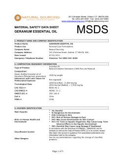


© Copyright 2026