1. No category

CHAPTER 9
Sequences of Functions
1. Pointwise Convergence
We have accumulated much experience working with sequences of numbers. The
next level of complexity is sequences of functions. This chapter explores several ways
that sequences of functions can converge to another function. The basic starting
point is contained in the following definitions.
Definition 9.1. Suppose S ⇢ R and for each n 2 N there is a function
fn : S ! R. The collection {fn : n 2 N} is a sequence of functions defined on S.
For each fixed x 2 S, fn (x) is a sequence of numbers, and it makes sense to ask
whether this sequence converges. If fn (x) converges for each x 2 S, a new function
f : S ! R is defined by
f (x) = lim fn (x).
n!1
The function f is called the pointwise limit of the sequence fn , or, equivalently, it is
S
said fn converges pointwise to f . This is abbreviated fn !f , or simply fn ! f , if
the domain is clear from the context.
Example 9.1. Let
Then fn ! f where
8
>
<0,
fn (x) = xn ,
>
:
1,
f (x) =
(
0,
1,
x<0
0x<1.
x 1
x<1
.
x 1
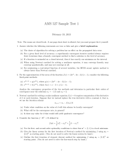
(See Figure 1.) This example shows that a pointwise limit of continuous functions
need not be continuous.
Example 9.2. For each n 2 N, define fn : R ! R by
nx
fn (x) =
.
1 + n2 x 2
(See Figure 2.) Clearly, each fn is an odd function and lim|x|!1 fn (x) = 0. A bit
of calculus shows that fn (1/n) = 1/2 and fn ( 1/n) = 1/2 are the extreme values
of fn . Finally, if x 6= 0,
|fn (x)| =
nx
nx
1
< 2 2 =
1 + n2 x 2
n x
nx
implies fn ! 0. This example shows that functions can remain bounded away from
0 and still converge pointwise to 0.
9-1
9-2
CHAPTER 9. SEQUENCES OF FUNCTIONS
1.0
0.8
0.6
0.4
0.2
0.2
0.4
0.6
0.8
1.0
Figure 1. The first ten functions from the sequence of Example 9.1.
0.4
0.2
!3
!2
1
!1
2
3
!0.2
!0.4
Figure 2. The first four functions from the sequence of Example 9.2.
Example 9.3. Define fn : R ! R by
8
2n+4
>
x 2n+3 ,
<2
fn (x) =
22n+4 x + 2n+4 ,
>
:
0,
1
2n+1
3
2n+2
<x<
x<
otherwise
3
2n+2
1
2n
To figure out what this looks like, it might help to look at Figure 3.
The graph of fn is a piecewise linear function supported on [1/2n+1 , 1/2n ] and
the
R 1 area under the isosceles triangle of the graph over this interval is 1. Therefore,
f = 1 for all n.
0 n
If x > 0, then whenever x > 1/2n , we have fn (x) = 0. From this it follows that
fn ! 0.
The Rlesson to
R 1be learned from this example is that it may not be true that
1
limn!1 0 fn = 0 limn!1 fn .
Example 9.4. Define fn : R ! R by
(
n 2
x +
fn (x) = 2
|x|,
May 8, 2015
1
2n ,
|x| 
|x| >
1
n
1
n
.
http://math.louisville.edu/⇠lee/ira
Pointwise and Uniform Convergence
9-3
64
32
16
8
1 1
16 8
1
4
1
2
1
Figure 3. The first four functions fn ! 0 from the sequence of Example 9.3.
1/2
1/4
1/8
1
1
Figure 4. The first ten functions of the sequence fn ! |x| from
Example 9.4.
(See Figure 4.) The parabolic section in the center was chosen so fn (±1/n) = 1/n
and fn0 (±1/n) = ±1. This splices the sections together at (±1/n, ±1/n) so fn is
di↵erentiable everywhere. It’s clear fn ! |x|, which is not di↵erentiable at 0.
This example shows that the limit of di↵erentiable functions need not be
di↵erentiable.
The examples given above show that continuity, integrability and di↵erentiability
are not preserved in the pointwise limit of a sequence of functions. To have any
hope of preserving these properties, a stronger form of convergence is needed.
May 8, 2015
http://math.louisville.edu/⇠lee/ira
9-4
CHAPTER 9. SEQUENCES OF FUNCTIONS
2. Uniform Convergence
Definition 9.2. The sequence fn : S ! R converges uniformly to f : S ! R
on S, if for each " > 0 there is an N 2 N so that whenever n N and x 2 S, then
|fn (x) f (x)| < ".
S
In this case, we write fn ◆
f , or simply fn ◆ f , if the set S is clear from the
context.
f(x) + ε
f(x)
fn(x)
f(x
a
ε
b
Figure 5. |fn (x)
f (x)| < " on [a, b], as in Definition 9.2.
The di↵erence between pointwise and uniform convergence is that with pointwise
convergence, the convergence of fn to f can vary in speed at each point of S. With
uniform convergence, the speed of convergence is roughly the same all across S.
Uniform convergence is a stronger condition to place on the sequence fn than
pointwise convergence in the sense of the following theorem.
S
S
Theorem 9.3. If fn ◆
f , then fn !f .
Proof. Let x0 2 S and " > 0. There is an N 2 N such that when n N , then
|f (x) fn (x)| < " for all x 2 S. In particular, |f (x0 ) fn (x0 )| < " when n N .
This shows fn (x0 ) ! f (x0 ). Since x0 2 S is arbitrary, it follows that fn ! f . ⇤
The first three examples given above show the converse to Theorem 9.3 is false.
There is, however, one interesting and useful case in which a partial converse is true.
S
Definition 9.4. If fn !f and fn (x) " f (x) for all x 2 S, then fn increases to
S
f on S. If fn !f and fn (x) # f (x) for all x 2 S, then fn decreases to f on S. In
either case, fn is said to converge to f monotonically.
The functions of Example 9.4 decrease to |x|. Notice that in this case, the
convergence is also happens to be uniform. The following theorem shows Example
9.4 to be an instance of a more general phenomenon.
Theorem 9.5 (Dini’s Theorem). If
(a) S is compact,
S
(b) fn !f monotonically,
(c) fn 2 C(S) for all n 2 N, and
(d) f 2 C(S),
then fn ◆ f .
May 8, 2015
http://math.louisville.edu/⇠lee/ira
3. METRIC PROPERTIES OF UNIFORM CONVERGENCE
9-5
Proof. There is no loss of generality in assuming fn # f , for otherwise we
consider fn and f . With this assumption, if gn = fn f , then gn is a sequence
of continuous functions decreasing to 0. It suffices to show gn ◆ 0.
To do so, let " > 0. Using continuity and pointwise convergence, for each x 2 S
find an open set Gx containing x and an Nx 2 N such that gNx (y) < " for all y 2 Gx .
Notice that the monotonicity condition guarantees gn (y) < " for every y 2 Gx and
n Nx .
The collection {Gx : x 2 S} is an open cover for S, so it must contain a finite
subcover {Gxi : 1  i  n}. Let N = max{Nxi : 1  i  n} and choose m N . If
x 2 S, then x 2 Gxi for some i, and 0  gm (x)  gN (x)  gNi (x) < ". It follows
that gn ◆ 0.
⇤
1
fn (x) = xn
1/2
2
1/n
1
Figure 6. This shows a typical function from the sequence of Example 9.5.
Example 9.5. Let fn (x) = xn for n 2 N, then fn decreases to 0 on [0, 1). If
0 < a < 1 Dini’s Theorem shows fn ◆ 0 on the compact interval [0, a]. On the
whole interval [0, 1), fn (x) > 1/2 when 2 1/n < x < 1, so fn is not uniformly
convergent. (Why doesn’t this violate Dini’s Theorem?)
3. Metric Properties of Uniform Convergence
If S ⇢ R, let B(S) = {f : S ! R : f is bounded}. For f 2 B(S), define
kf kS = lub {|f (x)| : x 2 S}. (It is abbreviated to kf k, if the domain S is clear from
the context.) Apparently, kf k 0, kf k = 0 () f ⌘ 0 and, if g 2 B(S), then
kf gk = kg f k. Moreover, if h 2 B(S), then
kf
gk = lub {|f (x)
 lub {|f (x)
 lub {|f (x)
= kf
May 8, 2015
g(x)| : x 2 S}
h(x)| + |h(x)
g(x)| : x 2 S}
h(x)| : x 2 S} + lub {|h(x)
hk + kh
gk
g(x)| : x 2 S}
http://math.louisville.edu/⇠lee/ira
9-6
CHAPTER 9. SEQUENCES OF FUNCTIONS
Combining all this, it follows that kf gk is a metric1 on B(S).
The definition of uniform convergence implies that for a sequence of bounded
functions fn : S ! R,
fn ◆ f () kfn f k ! 0.
Because of this, the metric kf gk is often called the uniform metric or the supmetric. Many ideas developed using the metric properties of R can be carried over
into this setting. In particular, there is a Cauchy criterion for uniform convergence.
Definition 9.6. Let S ⇢ R. A sequence of functions fn : S ! R is a Cauchy
sequence under the uniform metric, if given " > 0, there is an N 2 N such that when
m, n N , then kfn fm k < ".
Theorem 9.7. Let fn 2 B(S). There is a function f 2 B(S) such that fn ◆ f
i↵ fn is a Cauchy sequence in B(S).
Proof. ()) Let fn ◆ f and " > 0. There is an N 2 N such that n
N
implies kfn f k < "/2. If m N and n N , then
" "
kfm fn k  kfm f k + kf fn k < + = "
2 2
shows fn is a Cauchy sequence.
(() Suppose fn is a Cauchy sequence in B(S) and " > 0. Choose N 2 N so
that when kfm fn k < " whenever m N and n N . In particular, for a fixed
x0 2 S and m, n
N , |fm (x0 ) fn (x0 )|  kfm fn k < " shows the sequence
fn (x0 ) is a Cauchy sequence in R and therefore converges. Since x0 is an arbitrary
point of S, this defines an f : S ! R such that fn ! f .
Finally, if m, n N and x 2 S the fact that |fn (x) fm (x)| < " gives
|fn (x)
f (x)| = lim |fn (x)
m!1
N , then kfn
This shows that when n
fn ◆ f .
fm (x)|  ".
f k  ". We conclude that f 2 B(S) and
⇤
A collection of functions S is said to be complete under uniform convergence,
if every Cauchy sequence in S converges to a function in S. Theorem 9.7 shows
B(S) is complete under uniform convergence. We’ll see several other collections of
functions that are complete under uniform convergence.
Example 9.6. For S ⇢ R let L(S) be all the functions f : S ! R such that
f (x) = mx + b for some constants m and b. In particular, let fn be a Cauchy
sequence in L([0, 1]). Theorem 9.7 shows there is an f : [0, 1] ! R such that fn ◆ f .
In order to show L([0, 1]) is complete, it suffices to show f 2 L([0, 1]).
To do this, let fn (x) = mn x + bn for each n. Then fn (0) = bn ! f (0) and
mn = fn (1)
Given any x 2 [0, 1],
fn (x)
((f (1)
bn ! f (1)
f (0))x + f (0)) = mn x + bn
= (mn
This shows f (x) = (f (1)
complete.
(f (1)
f (0).
((f (1)
f (0))x + f (0))
f (0)))x + bn
f (0) ! 0.
f (0))x + f (0) 2 L([0, 1]) and therefore L([0, 1]) is
1Definition 2.10
May 8, 2015
http://math.louisville.edu/⇠lee/ira
4. SERIES OF FUNCTIONS
9-7
Example
Pn 9.7. Let P = {p(x) : p is a polynomial}. The sequence of polynomials
pn (x) = k=0 xk /k! increases to ex on [0, a] for any a > 0, so Dini’s Theorem shows
pn ◆ ex on [0, a]. But, ex 2
/ P, so P is not complete. (See Exercise 7.25.)
4. Series of Functions
The definitions of pointwiseP
and uniform convergence are extended in the natural
1
way to series of functions. If k=1 fk is a series of functions defined on a set S,
then the series converges
Pnpointwise or uniformly, depending on whether the sequence
of partial sums, sn = k=1 fk converges pointwise or uniformly,
P1 respectively. It is
absolutely convergent or absolutely uniformly convergent, if n=1 |fn | is convergent
or uniformly convergent on S, respectively.
The following theorem is obvious and its proof is left to the reader.
P1
P1
Theorem 9.8. Let n=1 fn be a series of functions
P1 defined on S. If n=1 fn
is absolutely convergent, then it is convergent. If n=1 fn is absolutely uniformly
convergent, then it is uniformly convergent.
The following theorem is a restatement of Theorem 9.5 for series.
P1
Theorem 9.9. If
n=1 fn is a series of nonnegative continuous functions
P1
converging pointwise to a continuous function on a compact set S, then n=1 fn
converges uniformly on S.
A simple, but powerful technique for showing uniform convergence of series is
the following.
Theorem 9.10 (Weierstrass M-Test). If fn : S ! R is a sequence of functions
and P
Mn is a sequence nonnegative
P1 numbers such that kfn kS  Mn for all n 2 N
1
and n=1 Mn converges, then n=1 fn is absolutely uniformly convergent.
P1
Proof. Let " > 0 and sn be the sequence of partial sums of n=1 |fn |. Using
the Cauchy criterion
Pnfor convergence of a series, choose an N 2 N such that when
n > m N , then k=m Mk < ". So,
ksn
sm k = k
n
X
k=m+1
fk k 
n
X
k=m+1
kfk k 
n
X
Mk < ".
k=m
This shows sn is a Cauchy sequence and must converge according to Theorem 9.7.
⇤
Example 9.8. Let a > 0 and Mn = an /n!. Since
Mn+1
a
= lim
= 0,
n!1 Mn
n!1 n + 1
lim
the Ratio Test shows
P1
n=0
Mn converges. When x 2 [ a, a],
xn
an

.
n!
n!
P1
The Weierstrass M-Test now implies n=0 xn /n! converges absolutely uniformly on
[ a, a] for any a > 0. (See Exercise 9.4.)
May 8, 2015
http://math.louisville.edu/⇠lee/ira
9-8
CHAPTER 9. SEQUENCES OF FUNCTIONS
5. Continuity and Uniform Convergence
Theorem 9.11. If fn : S ! R is such that each fn is continuous at x0 and
S
fn ◆
f , then f is continuous at x0 .
Proof. Let " > 0. Since fn ◆ f , there is an N 2 N such that whenever n N
and x 2 S, then |fn (x) f (x)| < "/3. Because fN is continuous at x0 , there is a
> 0 such that x 2 (x0
, x0 + ) \ S implies |fN (x) fN (x0 )| < "/3. Using these
two estimates, it follows that when x 2 (x0
, x0 + ) \ S,
|f (x)
f (x0 )| = |f (x)
 |f (x)
fN (x) + fN (x)
fN (x)| + |fN (x)
< "/3 + "/3 + "/3 = ".
fN (x0 ) + fN (x0 )
f (x0 )|
fN (x0 )| + |fN (x0 )
f (x0 )|
⇤
Therefore, f is continuous at x0 .
The following corollary is immediate from Theorem 9.11.
Corollary 9.12. If fn is a sequence of continuous functions converging uniformly to f on S, then f is continuous.
Example 9.1 shows that continuity is not preserved under pointwise convergence.
Corollary 9.12 establishes that if S is compact, then C(S) is complete under the
uniform metric.
The fact that C([a, b]) is closed under uniform convergence is often useful
because, given a “bad” function f 2 C([a, b]), it’s often possible to find a sequence
fn of “good” functions in C([a, b]) converging uniformly to f . Following is the most
widely used theorem of this type.
Theorem 9.13 (Weierstrass Approximation Theorem). If f 2 C([a, b]), then
there is a sequence of polynomials pn ◆ f .
To prove this theorem, we first need a lemma.
⇣R
⌘
1
2 n
Lemma 9.14. For n 2 N let cn =
(1
t
)
dt
1
kn (t) =
(
cn (1
0,
t2 ) n ,
1
and
|t|  1
.
|t| > 1
(See Figure 7.) Then
(a) kn (t) 0 for all t 2 R and n 2 N;
R1
(b)
k = 1 for all n 2 N; and,
1 n
(c) if 0 < < 1, then kn ◆ 0 on ( 1,
] [ [ , 1).
Proof. Parts (a) and (b) follow easily from the definition of kn .
To prove (c) first note that
✓
◆n
Z 1
Z 1/pn
2
1
2 n
p
1=
kn
cn (1 t ) dt cn
1
.
p
n
n
1
1/ n
May 8, 2015
http://math.louisville.edu/⇠lee/ira
5. CONTINUITY AND UNIFORM CONVERGENCE
9-9
1.2
1.0
0.8
0.6
0.4
0.2
!1.0
0.5
!0.5
1.0
Figure 7. Here are the graphs of kn (t) for n = 1, 2, 3, 4, 5.
Since 1 n1
2 (0, 1) and
n
p
" 1e , it follows there is an ↵ > 0 such that cn < ↵ n.2 Letting
 t  1,
p
2 n
kn (t)  kn ( )  ↵ n(1
) !0
by L’Hospital’s Rule. Since kn is an even function, this establishes (c).
⇤
A sequence of functions satisfying conditions such as those in Lemma 9.14 is
called a convolution kernel or a Dirac sequence.3 Several such kernels play a key
role in the study of Fourier series, as we will see in Theorems 10.5 and 10.13. The
one defined above is called the Landau kernel.4
We now turn to the proof of the theorem.
Proof. There is no generality lost in assuming [a, b] = [0, 1], for otherwise we
consider the linear change of variables g(x) = f ((b a)x+a). Similarly, we can assume
f (0) = f (1) = 0, for otherwise we consider g(x) = f (x) ((f (1) f (0))x f (0),
which is a polynomial added to f . We can further assume f (x) = 0 when x 2
/ [0, 1].
Set
Z 1
(81)
pn (x) =
f (x + t)kn (t) dt.
1
To see pn is a polynomial, change variables in the integral using u = x + t to arrive
at
Z x+1
Z 1
pn (x) =
f (u)kn (u x) du =
f (u)kn (x u) du,
x 1
0
2Repeated application of integration by parts shows
n + 1/2
n 1/2
n 3/2
3/2
(n + 3/2)
⇥
⇥
⇥ ··· ⇥
= p
.
n
n 1
n 2
1
⇡ (n + 1)
p
With the aid of Stirling’s formula, it can be shown cn ⇡ 0.565 n.
3Given two functions f and g defined on R, the convolution of f and g is the integral
Z 1
f ? g(x) =
f (t)g(x t) dt.
cn =
1
The term convolution kernel is used because such kernels typically replace g in the convolution
given above, as can be seen in the proof of the Weierstrass approximation theorem.
4
It was investigated by the German mathematician Edmund Landau (1877–1938).
May 8, 2015
http://math.louisville.edu/⇠lee/ira
9-10
CHAPTER 9. SEQUENCES OF FUNCTIONS
because f (x) = 0 when x 2
/ [0, 1]. Notice that kn (x u) is a polynomial in u with
coefficients being polynomials in x, so integrating f (u)kn (x u) yields a polynomial
in x. (Just try it for a small value of n and a simple function f !)
Use (81) and Lemma 9.14(b) to see for 2 (0, 1) that
Z 1
(82) |pn (x) f (x)| =
f (x + t)kn (t) dt f (x)
1
=
=

Z
Z
Z
1
(f (x + t)
f (x))kn (t) dt
|f (x + t)
f (x)|kn (t) dt
1
1
|f (x + t)
1
f (x)|kn (t) dt +
Z
<|t|1
|f (x + t)
f (x)|kn (t) dt.
We’ll handle each of the final integrals in turn.
Let " > 0 and use the uniform continuity of f to choose a 2 (0, 1) such that
when |t| < , then |f (x + t) f (x)| < "/2. Then, using Lemma 9.14(b) again,
Z
Z
"
"
(83)
|f (x + t) f (x)|kn (t) dt <
kn (t) dt <
2
2
According to Lemma 9.14(c), there is an N 2 N so that when n
"
then kn (t) < 8(kf k+1)(1
) . Using this, it follows that
(84)
Z
<|t|1
=
Z
|f (x + t)
1
,
f (x)|kn (t) dt
|f (x + t)
 2kf k
< 2kf k
N and |t|
f (x)|kn (t) dt +
Z
"
8(kf k + 1)(1
1
Z
1
|f (x + t)
kn (t) dt + 2kf k
)
(1
Z
) + 2kf k
f (x)|kn (t) dt
1
kn (t) dt
"
8(kf k + 1)(1
)
(1
)=
"
2
Combining (83) and (84), it follows from (82) that |pn (x) f (x)| < " for all x 2 [0, 1]
and pn ◆ f .
⇤
Corollary 9.15. If f 2 C([a, b]) and " > 0, then there is a polynomial p such
that kf pk[a,b] < ".
The theorems of this section can also be used to construct some striking examples
of functions with unwelcome behavior. Following is perhaps the most famous.
Example 9.9. There is a continuous f : R ! R that is di↵erentiable nowhere.
Proof. Thinking of the canonical example of a continuous function that fails to
be di↵erentiable at a point—the absolute value function—we start with a “sawtooth”
function. (See Figure 8.)
(
x 2n,
2n  x < 2n + 1, n 2 Z
s0 (x) =
2n + 2 x, 2n + 1  x < 2n + 2, n 2 Z
May 8, 2015
http://math.louisville.edu/⇠lee/ira
5. CONTINUITY AND UNIFORM CONVERGENCE
9-11
Notice that s0 is continuous and periodic with period 2 and maximum value 1.
Compress it both vertically and horizontally:
✓ ◆n
3
sn (x) =
s0 (4n x) , n 2 N.
4
Each sn is continuous and periodic with period pn = 2/4n and ksn k = (3/4)n .
1.0
0.8
0.6
0.4
0.2
0.5
1.0
1.5
2.0
2.5
3.0
3.5
Figure 8. s0 , s1 and s2 from Example 9.9.
Finally, the desired function is
f (x) =
1
X
sn (x).
n=0
Since ksn k = (3/4)n , the Weierstrass M -test implies the series defining f is
uniformly convergent and Corollary 9.12 shows f is continuous on R. We will show
f is di↵erentiable nowhere.
Let x 2 R, m 2 N and hm = 1/(2 · 4m ).
If n > m, then hm /pn = 4n m 1 2 N, so sn (x ± hm ) sn (x) = 0 and
m
f (x ± hm ) f (x) X sk (x ± hm ) sk (x)
=
.
±hm
±hm
(85)
k=0
On the other hand, if n < m, then a worst-case estimate is that
✓ ◆n ✓ ◆
sn (x ± hm ) sn (x)
3
1

/
= 3n .
hm
4
4n
3.0
2.5
2.0
1.5
1.0
0.5
0.5
1.0
1.5
2.0
Figure 9. The nowhere di↵erentiable function f from Example 9.9.
May 8, 2015
http://math.louisville.edu/⇠lee/ira
9-12
CHAPTER 9. SEQUENCES OF FUNCTIONS
This gives
m
X1
k=0
m
X1 sk (x ± hm ) sk (x)
sk (x ± hm ) sk (x)

±hm
±hm
k=0
3m 1
3m
(86)

<
.
3 1
2
Since sm is linear on intervals of length 4 m = 2 · hm with slope ±3m on those
linear segments, at least one of the following is true:
sm (x + hm )
hm
(87)
s(x)
sm (x
= 3m or
hm )
hm
s(x)
= 3m .
Suppose the first of these is true. The argument is essentially the same in the second
case.
Using (85), (86) and (87), the following estimate ensues
f (x + hm )
hm
f (x)
=
=
1
X
sk (x + hm )
k=0
m
X
k=0
sk (x)
hm
sk (x + hm )
hm
sm (x + hm )
hm
sk (x)
sm (x)
m
X1
k=0
3m
3m
>3
=
.
2
2
Since 3m /2 ! 1, it is apparent f 0 (x) does not exist.
sk (x ± hm ) sk (x)
±hm
m
⇤
There are many other constructions of nowhere di↵erentiable continuous functions. The first was published by Weierstrass [20] in 1872, although it was known
in the folklore sense among mathematicians earlier than this. (There is an English
translation of Weierstrass’ paper in [10].) In fact, it is now known in a technical
sense that the “typical” continuous function is nowhere di↵erentiable [4].
6. Integration and Uniform Convergence
One of the recurring questions with integrals is when it is true that
Z
Z
lim
fn =
lim fn .
n!1
n!1
This is often referred to as “passing the limit through the integral.” At some point
in her career, any student of advanced analysis or probability theory will be tempted
to just blithely pass the limit through. But functions such as those of Example
9.3 show that some care is needed. A common criterion for doing so is uniform
convergence.
Rb
Theorem 9.16. If fn : [a, b] ! R such that a fn exists for each n and fn ◆ f
on [a, b], then
Z b
Z b
f = lim
fn
.
May 8, 2015
a
n!1
a
http://math.louisville.edu/⇠lee/ira
6. INTEGRATION AND UNIFORM CONVERGENCE
9-13
Proof. Some care must be taken in this proof, because there are actually two
things to prove. Before the equality can be shown, it must be proved that f is
integrable.
To show that f is integrable, let " > 0 and N 2 N such that kf fN k < "/3(b a).
If P 2 part ([a, b]), then
|R (f, P, x⇤k )
(88)
R (fN , P, x⇤k ) | = |
=|

n
X
k=1
N
X
f (x⇤k )|Ik |
(f (x⇤k )
k=1
|f (x⇤k )
k=1
fN (x⇤k )|Ik ||
fN (x⇤k ))|Ik ||
k=1
N
X
n
X
fN (x⇤k )||Ik |
n
X
"
|Ik |
3(b a))
k=1
"
=
3
According to Theorem 8.10, there is a P 2 part ([a, b]) such that whenever
P ⌧ Q1 and P ⌧ Q2 , then
"
(89)
|R (fN , Q1 , x⇤k ) R (fN , Q2 , yk⇤ ) | < .
3
Combining (88) and (89) yields
<
|R (f, Q1 , x⇤k )
R (f, Q2 , yk⇤ )|
= |R (f, Q1 , x⇤k )
 |R (f, Q1 , x⇤k )
R (fN , Q1 , x⇤k ) + R (fN , Q1 , x⇤k )
R (fN , Q1 , x⇤k ) + R (fN , Q2 , yk⇤ )
R (fN , Q1 , x⇤k )| + |R (fN , Q1 , x⇤k )
R (f, Q2 , yk⇤ )|
R (fN , Q1 , x⇤k )|
+ |R (fN , Q2 , yk⇤ )
R (f, Q2 , yk⇤ )|
" " "
< + + ="
3 3 3
Another application of Theorem 8.10 shows that f is integrable.
Finally, when n N ,
Z b
Z b
Z b
Z b
"
"
f
fn =
(f fn ) <
= <"
3(b
a)
3
a
a
a
a
Rb
Rb
shows that a fn ! a f .
⇤
P1
Corollary 9.17. If n=1 fn is a series of integrable functions converging
uniformly on [a, b], then
Z bX
1
1 Z b
X
fn =
fn
a n=1
n=1
a
Example 9.10. It was shown in Example 4.2 that the geometric series
1
X
1
tn =
,
1 < t < 1.
1 t
n=0
May 8, 2015
http://math.louisville.edu/⇠lee/ira