1. science
2. mathematics
3. geometry

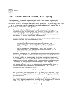
FUNCTION PROJECTIVE SYNCHRONIZATION OF A
NEW HYPER CHAOTIC SYSTEM
Priyambada Tripathi
Research Scholar
Department of Mathematics
University of Delhi, Delhi 110007
India
[email protected]
1. Introduction
• In this article a function projective synchronization(FPS) of two
identical new hyper chaotic systems is defined and scheme of FPS
is developed by using Open-Plus-Closed-Looping(OPCL) coupling
method. A new hyper chaotic system has been constructed and
then response system with parameters perturbation has been defined. Numerical simulations verify the effectiveness of this scheme,
which has been performed by mathematica and MATLAB.
• Here, we have constructed a new hyper chaotic system and verified
the chaotic behavior of this system by time series analysis and drawing chaotic attractors via mathematica and MATLAB. Hyperchaotic
behavior of this system is discovered within some system parameters
range, which has not yet been reported previously.
2. Preliminaries
In this section we mention some definitions and scheme of the main task.
• Chaos is a dynamical regime in which a system becomes extremely
sensitive to initial conditions and reveals an unpredictable and randomlike behavior. Small differences in initial conditions yield widely diverging outcomes for chaotic systems, rendering long term prediction
impossible in general.
• A hyperchaotic system is defined as chaotic behavior with at least
two positive Lyapunov exponents.
2.1. Function Projective Synchronization. Function Projective
synchronization is defined in the following manner:
Let x˙ = F (x, t) be the drive chaotic system, and y˙ = F (y, t) + U be the
response system, where x = (x1 (t), x2 (t), ..., xm (t))T ,
1
2
FUNCTION PROJECTIVE SYNCHRONIZATION
y = (y1 (t), y2 (t), ..., ym (t))T , U = (u1 (x, y), u2 (x, y), ..., um (x, y)) is a
controller to be determined later.
Denote ei = xi − fi (x)yi , (i = 1, 2, ..., m), fi (x), (i = 1, 2, ..., m) are
functions of x. If
lim ∥e∥ = 0,
t→∞
e = (e1 , e2 , ..., em ), there exists function projective synchronization (FPS)
between these two identical chaotic (hyperchaotic) systems, and we call f
a scaling function matrix.
2.2. Methodology for FPS via OPCL. Here, we will construct
corresponding response system through the OPCL coupling method.
Consider the following n-dimensional chaotic system as drive system
dx
dt
= f (x) + △f (x),
(1)
where x ∈ Rn and △f (x) is the perturbation part of the parameters. Now,
consider the following n-dimensional chaotic system as response system
according to coupling method :
dy
= f (y) + D(y, g),
dt
(2)
where y ∈ Rn . The coupling function is:
D(y, g) = g˙ − f (g) + (H −
∂f (g)
)(y − g)
∂g
(3)
where ∂f∂g(g) is the jacobian matrix of the dynamics system. H is an n×n
Hurwitz constant matrix, whose eigen values are negative and g = β(t)x
with β(t) is a scaling function which is continuously differentiable. When
β(t) = ±1, system is complete synchronization or antisynchronization
accordingly.
Our goal in this paper is to find out D(y, g) and hence find error dynamics
of the system such that
lim ∥e∥ = lim ∥y − g∥ = 0,
t→∞
t→∞
where ∥ · ∥ is the Euclidean norm, then the systems (1) and (2) are said to
be Function Projective synchronized.
3. System Description
3.1. Hyper Chaotic Rabinovich-Fabrikant system. The
Rabinovich-Fabrikant chaotic system is a set of three coupled ordinary
differential equations exhibiting chaotic behavior for certain values of
parameters. They are named after Mikhail Rabinovich and Anatoly
FUNCTION PROJECTIVE SYNCHRONIZATION
3
Fabrikant, who described them in 1979 [18]. The equations of system are :

x˙1 = x2 (x3 − 1 + x21 )+γx1 , 


2
x˙2 = x1 (3x3 + 1 − x1 )+γx2 ,



x˙3 = −2x3 (x1 x2 +α)
where α and γ are constant parameters that control the evolution of the
system. For some values of α and γ, the system is chaotic but for other it
tends to a stable periodic orbit. Now, we construct a new hyper chaotic
system by introducing one more differential equation with a new
parameter δ in the above system as follow:

x˙1 = x2 (x3 − 1 + x21 )+γx1 , 



2

x˙ = x (3x + 1 − x )+γx , 
2
1
3
2
1
x˙3 = −2x3 (x1 x2 +α),
x˙4 = −3x3 (x2 x4 + δ) + x24






(4)
This new system shows hyper chaotic behavior with some values of
parameters and tend to stable periodic orbits with other values of
parameters. We have investigated system’s behavior for different values of
δ. Figures are given below:
0.0
0.5
1.0
1.5
0.0
0.2
0.4
-1.4
-1.3
-1.2
-1.1
-1.0
Fig.1 Chaotic behavior of the
system with α = 0.14,γ = 1.1
and −0.01 ≤ δ ≤ 7650 tending to
stable periodic orbits
4
FUNCTION PROJECTIVE SYNCHRONIZATION
1.5
-1.0
-1.1
1.0
-1.2
0.5
-1.3
20
20
40
60
80
40
60
80
100
100
Fig.2 Time series analysis of y1[t] Fig.3 Time series analysis of y2[t]
with α = 0.14,γ = 1.1 and
with α = 0.14,γ = 1.1 and
−0.01 ≤ δ ≤ 7650
−0.01 ≤ δ ≤ 7650
0.5
20
40
60
80
100
0.4
-20
0.3
-40
0.2
-60
0.1
-80
-100
20
40
60
80
100
Fig.4 Time series analysis of y3[t] Fig.5 Time series analysis of y4[t]
with α = 0.14,γ = 1.1 and
with α = 0.14,γ = 1.1 and
−0.01 ≤ δ ≤ 7650
−0.01 ≤ δ ≤ 7650
1.5
1.0
0.5
0.0
0.4
0.2
0.0
-1.4
-1.3
-1.2
-1.1
-1.0
Fig.6 Chaotic Behavior of the
system with α = 0.87,γ = 1.1
and δ = 1890
FUNCTION PROJECTIVE SYNCHRONIZATION
5
-0.4
2.0
-0.6
-0.8
1.5
-1.0
1.0
-1.2
-1.4
0.5
-1.6
20
40
60
80
20
100
40
60
80
100
Fig.7 Time series analysis of y1[t] Fig.8 Time series analysis of y2[t]
with α = 0.87,γ = 1.1 and
with α = 0.87,γ = 1.1 and
δ = 1890
δ = 1890
20
1.2
1.0
40
60
80
100
-20
0.8
-40
0.6
0.4
-60
0.2
-80
20
40
60
80
100
Fig.9 Time series analysis of y3[t]
with α = 0.87,γ = 1.1 and
δ = 1890
Fig.10 Time series analysis of
y4[t] with α = 0.87,γ = 1.1 and
δ = 1890
2
1
0
1.0
0.5
0.0
-1.5
-1.0
-0.5
Fig.11 Chaotic Behavior of the
system with α = 0.87,γ = 1.1
and δ = −0.2
6
FUNCTION PROJECTIVE SYNCHRONIZATION
-0.4
2.0
-0.6
-0.8
1.5
-1.0
1.0
-1.2
-1.4
0.5
-1.6
20
40
60
80
20
100
Fig.12 Time series analysis of
y1[t] with α = 0.87,γ = 1.1 and
δ = −0.2
40
60
80
100
Fig.13 Time series analysis of
y2[t] with α = 0.87,γ = 1.1 and
δ = −0.2
0.6
1.2
0.5
1.0
0.8
0.4
0.6
0.3
0.4
0.2
0.2
20
40
60
80
100
Fig.14 Time series analysis of
y3[t] with α = 0.87,γ = 1.1 and
δ = −0.2
20
40
60
80
100
Fig.15 Time series analysis of
y4[t] with α = 0.87,γ = 1.1 and
δ = −0.2
3.2. Illustration. In this section, we perform function projective
synchronization of above described system via OPCL coupling method.
Define following system as a drive system with parameters perturbation as

x˙1 = x2 (x3 − 1 + x21 ) + (γ + ∆γ)x1 , 




x˙ = x (3x − x2 + 1) + (γ + ∆γ)x , 
2
1
3
2
1
(5)






x˙3 = −2x3 (x1 x2 +α + ∆α),
x˙4 = −3x3 (x2 x4 + δ + ∆δ) + x24
where ∆γ, ∆α and ∆δ are the perturbation parts in the parameters. Now
construct the corresponding response system via OPCL coupling method.
The Jacobian matrix of the system (5) is

γ + ∆γ + 2x1 x2 x21 + x3 − 1
2
∂f (x) 
 3x3 − 3x1 + 1
=
∂x

−2x2 x3
0
x2
0
γ + ∆γ
3x1
0
−2x1 x3
−2(α + ∆α + x1 x2 )
0
−3x3 x4
−3x2 x4 − 3δ − 3∆δ
2x4 − 3x2 x3





FUNCTION PROJECTIVE SYNCHRONIZATION
7
Define Hurwitz matrix H as the unit negative matrix −I (as g = βx),
Then H − ∂f∂g(g)



=


−γ − ∆γ − 2β 2 x1 x2 − 1
−3βx3 + 3β 2 x21 − 1
2β 2 x2 x3
0
−β 2 x21 − βx3 + 1
−βx2
0
−γ − ∆γ − 1
−3βx1
0
2β 2 x1 x3
2(α + ∆α + β 2 x1 x2 ) − 1
0
2
3β x3 x4
2
3β x2 x4 + 3δ + 3∆δ






−2βx4 + 3β 2 x2 x3 − 1
Therefore, response system after coupling is as follows
∂f (g1 )
)(y1 − g1 )
∂g1
∂f (g2 )
y˙2 = f (y2 ) − f (g2 ) + g˙2 + (H −
)(y2 − g2 )
∂g2
∂f (g3 )
y˙3 = f (y3 ) − f (g3 ) + g˙3 + (H −
)(y3 − g3 )
∂g3
∂f (g4 )
y˙4 = f (y4 ) − f (g4 ) + g˙4 + (H −
)(y4 − g4 )
∂g4
y˙1 = f (y1 ) − f (g1 ) + g˙1 + (H −












(6)











As error dynamics is defined as e˙ = y˙ − g,
˙ so we have final equation of
error dynamics after coupling and putting values of f(y),f(g) and
(H − ∂f∂g(g) )(y − g) in above equation as follows
e˙1 = ∆γe1 + e2 e3 + e2 e21 + 2βx1 e1 e2 + βx2 e21 − e1
e˙2 = ∆γe2 + 3e1 e3 + e31 + 3βx1 e21 − e2








e˙3 = −2∆αe3 − 2e1 e2 e3 + e2 e1 e2 βx3 − 2βx2 e1 e3 − 2βx1 e2 e3 − e3 




e˙4 = −3∆δe3 − 2e2 e3 e4 − 3e2 e4 βx3 − 3βx2 e4 e3 − 3βx4 e2 − e4
(7)
So, from the above error dynamics we can conclude that FPS between two
identical hyper chaotic system can be achieved.
4. Numerical Simulations
If Perturbation of Parameters of the response system of hyper chaotic
Rabinovich-Fabrikant system are zero and β = 0.5 with the initial
conditions of drive system [x1 (0), x2 (0), x3 (0), x4 (0)] = [0, 2, 0.5, −0.2] and
response systems [y1 (0), y2 (0), y3 (0), y4 (0)] = [0.5, 1, −0.1, −0.15]
respectively. So, the initial conditions for
[e1 (0), e2 (0), e3 (0), e4 (0)] = [0.5, 0, −0.35, −0.05] diagrams of convergence of
errors given below are the witness of achieving function projective
synchronization between master and slave system.
8
FUNCTION PROJECTIVE SYNCHRONIZATION
0.30
0.07
0.25
0.06
0.05
0.20
0.04
0.15
0.03
0.10
0.02
0.05
0.01
2
4
6
8
Fig.16 Convergence of error
e1 , t∈[0, 10]
2
4
6
2
10
8
4
6
8
10
Fig.17 Convergence error of
e2 , t∈[0, 10]
10
2
4
6
8
10
-0.01
-0.02
-0.02
-0.04
-0.03
-0.06
-0.04
-0.08
-0.05
-0.10
-0.06
Fig.18 Convergence of error
e3 , t∈[0, 10]
Fig.19 Convergence of error
e4 , t∈[0, 10]
Conclusion and benefits
Since hyperchaotic systems have the characteristics of high capacity, high
security and high efficiency, it has been studied with increasing interest in
the fields of non-linear circuits, secure communications, lasers, control,
synchronization, and so on. So we have studied Function Projective
Synchronization behavior for this new hyper chaotic systems, which is
offcourse more effective and useful in secure communication as FPS is
more useful in secure communication as compare to others because of its
unpredictability . The results are validated by numerical simulations using
mathematica. It has more advantage over other synchronization to
enhance security of communication and moreover as it is performed for
hyperchaotic system, which makes it more useful.
References
[1] Pikovsky A, Rosenblum M, Kurths J. Synchronization: A Universal Concept Nonlinear Science. Cambridge University Press, 2002.
[2] Glass L. Synchronization and rhythmic processes in physiology. Nature, 410:277,2001.
[3] Strogatz S. Sync. Hyperion, 2003.
[4] Pecora LM, Carroll TL. Synchronization in chaotic systems, Phys. Rev. Lett.
64(1990): 821–824.
[5] Liao TL, Lin SH. Adaptive control and synchronization of Lorenz systems, J. Franklin
Inst. 336(1999): 925937.
[6] Chen SH, Lu J. Synchronization of an uncertain unified system via adaptive control,
Chaos Solitons & Fractals 14(2002), 643–647.
[7] Ge ZM, and Chen YS. Adaptive synchronization of unidirectional and mutual coupled
chaotic systems, Chaos Solitons & Fractals 26(2005), 881–888.
[8] Wang C, Ge SS. Synchronization of two uncertain chaotic systems via adaptive backstepping, Int. J. Bifurcat. Chaos 11(2001), 17431751.
FUNCTION PROJECTIVE SYNCHRONIZATION
9
[9] Wang C, Ge SS. Adaptive synchonizaion of uncertain chaotic systems via adaptive
backstepping design, Chaos Solitons & Fractals 12(2001), 1199–11206.
[10] Tan X, Zhang J, Yang Y. Synchronizing chaotic systems using backstepping design,
Chaos Solitons & Fractals 16(2003): 37–45.
[11] Chen HK. Synchronization of two different chaotic system: a new system and each
of the dynamical systems Lorenz, Chen and Lu, Chaos Solitons & Fractals 25(2005),
1049–1056.
[12] Ho MC, Hung YC. Synchronization two different systems by using generalized active
control, Phys. Lett. A 301(2002), 424–428.
[13] Yassen MT. Chaos synchronization between two different chaotic systems using active
control, Chaos Solitons & Fractals 23(2005), 131–140.
[14] Park JH. Chaos synchronization between two different chaotic dynamical systems,
Chaos Solitons & Fractals 27(2006), 549–554.
[15] Chen HK. Global chaos synchronization of new chaoic systems via nonlinear control,
Chaos Solitons & Fractals 23(2005), 1245–1251.
[16] Ge ZM, Yu TC, Chen YS. Chaos synchronization of a horizontal platform system, J.
Sound Vibrat 268(2003), 731–749.
[17] Wen GL, Xu D. Observer-based control for full-state projective synchronization of a
general class of chaotic maps in any dimension, Phys. Lett. A 330(2004), 420–425.
[18] Rabinovich, Mikhail I. and Fabrikant, A. L. (1979). ”Stochastic Self- Modulation of
Waves in Nonequilibrium Media”. Sov. Phys. JETP 50: 311.
[19] Cenys, A., Tamasevicius, A. and Baziliauskas, A. (2003) Hyperchaos in coupled Colpitts oscillators, Chaos, Solitons and Fractals, Vol. 7, pp. 349-353.
[20] Hua, M. and Xua, Z. Adaptive feedback controller for projective synchronization,
Nonlinear Analysis: Real World Applications 9 (2008) 1253 –1260.
[21] Liu, J., Chen, S. H. and Lu, J.A. Projective synchronization in a unified chaotic
system and its control, Acta Phys. Sin 52 (2003) 1595-1599.
[22] Mainieri, R. and Rehacek, J. Projective synchronization in three-dimensional chaotic
systems, Phys. Rev. Lett. 82 (1999) 3042-3045.
[23] Xin L. and Yong C. Function Projective Synchronization of Two Identical New Hyperchaotic Systems, Commun. Theor. Phys. (Beijing, China) 48 (2007) pp. 864-870.