1. business and industrial

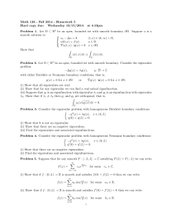
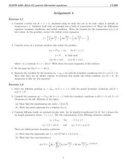
A note on existence and uniqueness of solutions for a 2D
bioheat problem with convective boundary conditions
Luciano Bedin
Ferm´ın S. Viloche Baz´an
∗
Department of Mathematics, Federal University of Santa Catarina
Florian´opolis SC, Santa Catarina, CEP 88040-900, Brazil
E-mail: [email protected], [email protected]
Abstract
We consider a 2D bioheat model on a domain with curvilinear polygonal boundary
and boundary conditions involving heat transfer between blood vessels and tissue. Based
on elliptic regularity on polygons and semigroup theory we obtain a Fourier series representation for the solution in H 2 settings. The results become useful in that they provide
theoretical support for numerical approaches recently published in literature.
Key words: Pennes equation, bioheat transfer, Fourier series, curvilinear polygons
1
Introduction
Modelling of thermal energy transport in living tissues has become crucial in applications
such as cancer treatment, burn therapy, cryosurgery, laser irradiation and others [6, 13, 17,
23, 25]. As a result, several analytical and numerical methods have appeared dealing with
initial boundary-value problems involving bioheat transfer equations for different geometries
and boundary conditions [18, 7, 9, 17, 25]. In particular, after the seminal paper by Pennes [20],
there have been several studies to characterize the thermal tissues properties, which gave rise
to various bioheat transfer equations with applications in distinct scenarios. However, despite
the efforts of researchers to analyze and describe solutions for certain problems in medical
applications, e.g., [1, 13, 24, 26, 23], rigorous analyses concerning existence and uniqueness are
still lacking. The goal of this note is to partially fill in this gap by providing a Fourier-based
analysis approach for a 2D bioheat transfer equation with convective boundary conditions on a
rectangle, whose numerical treatment and application in perfusion coefficient inverse estimation
problems has been given in [5, 7]; related work concerning inverse estimation problems involving
the bioheat model can be found in [6, 15, 16, 17, 25, 28]. Our existence and uniqueness analysis
is based on elliptic regularity theory on polygons in H 2 (O) settings for a domain O with
curvilinear polygonal boundary [14] and internal angles equal to π/2, along with semigroup
theory. By assuming so, our approach covers the traditional case where the tissue occupies a
rectangular region [17].
The rest of the note is organized as follows. In Section 2 the boundary conditions are taken
into account to transform the original problem into a standard Cauchy problem involving an
∗
The work of the second author is supported by CNPq, Brazil, grants 308709/2011-0, 477093/2011-6
1
elliptic operator. In Section 2 the spectral problem for the elliptic operator associated with
Pennes’ equation is solved and an analytical semigroup of contractions on L2 (O) is generated.
Proceeding this way, it is established not only a computable Fourier series representation for
the bioheat solution problem, but also a rigorous theoretical treatment is provided in order to
justify eigenfunction expansions methods very often seen in literature [7, 25]. In particular, a
highly accurate method for computing eigenvalues and eigenfunctions of the associated elliptic
operator is also introduced and illustrated by way of several numerical examples. The note
ends with some conclusions in Section 4.
Throughout the paper, H s (Ω) stands for the Sobolev space of functions with derivatives of
order less than or equal to s in L2 (Ω), with respective norm denoted by k.ks,2,Ω .
2
Bioheat equation
Let O ⊂ R2 denote an open, bounded and connected set with boundary Γ = ∪4i=1 Γi , where
Γi (the closure of the open arc Γi ) is a C ∞ curve [14]. Let si := Γi ∩ Γi+1 , 1 ≤ i ≤ 3,
s4 =: Γ4 ∩ Γ1 and assume that Γi follows Γi+1 in an anticlockwise direction. Also, assume that
for each 1 ≤ i ≤ 4, ωi = π/2, where ωi is the internal angle of the polygon with the vertex in si .
Let x = (x, y) and let ν i = (νx , νy ), τ i = (−νy , νx ) be the unit outward normal vector field to
Γi and the tangent vector field to Γi , respectively. The assumption on ωi is purely technical and
introduced to avoid the presence of singular solutions [3]. Let the temperature of a perfused
tissue occupying the region O be denoted by U = U (x, t) where t stands for the time variable.
The boundary Γ1 represents the upper skin surface, while the boundary Γ3 corresponds to a
wall between the tissue and an adjoint large blood vessel [7, 18]. The Pennes’ bioheat model
with convective boundary conditions we are interested is given by
ρc Ut − κ∆U + wb cb (U − Ua ) = qm + qe
∂U
= 0 on Γi ×]0, +∞[, i = 2, 4
∂ν i
∂U
κ
+ hU = hU∞ on Γ3 ×]0, +∞[,
∂ν 3
U = Ub on Γ1 ×]0, +∞[,
U = U0 in O × {0},
in O×]0, +∞[,
(1)
(2)
(3)
(4)
(5)
where ρ, c, h and κ are positive constants that stand for the density, the specific heat, the
heat transfer coefficient and the thermal conductivity of the tissue, respectively; cb is a positive
constant denoting the blood specific heat, wb is the mass flow rate of blood per unit volume
of tissue such that wb ≥ 0 a.e. in O, wb ∈ L∞ (O), and Ua ∈ L∞ (O) is the temperature of
arterial blood. Additionally, U0 ∈ L2 (O), Ub ∈ H 3/2 (Γ1 ) and U∞ ∈ H 1/2 (Γ3 ), are the initial
temperature of the tissue, the skin surface temperature and the environmental temperature (in
the adjacent blood vessel), respectively. Finally, for each T > 0, qm , qe ∈ C σ (]0, T ]; L2 (O)),
0 < σ < 1, stand for the metabolic heat generation per unit volume and the volumetric rate of
external heat, respectively. The boundary condition (3) attempts to simulate the heat transfer
between the tissue and the adjoint blood vessel in Γ3 , while (2) is an adiabatic condition. In
the upper skin surface the temperature is prescribed and gives rise to the boundary condition
(4).
The key idea behind our existence and uniqueness analysis is to transform the original initial
and boundary value problem problem (1)-(5) into a Cauchy problem through a suitable change
of variables involving a function Uext ∈ H 2 (O) satisfying (2)-(4). The existence proof of such
a function depends on mild conditions on function Ub (the skin surface temperature) and is
2
postponed to section 3 (see Lemma 3.4). In fact, setting V = U − Uext , the original problem
(1)-(5) can be expressed as
Vt + LV = f in O×]0, +∞],
∂V
= 0 on Γi ×]0, +∞[, i = 2, 4
∂ν i
∂V
κ
+ hV = 0 on Γ3 ×]0, +∞[,
∂ν 3
V = 0 on Γ1 ×]0, +∞[,
V = U0 − Uext in O × {0},
(6)
(7)
(8)
(9)
(10)
where L : A ⊂ L2 (O) → L2 (O) is the elliptic operator given by L = (ρc)−1 (−κ∆ + cb wb I),
with
A := {v ∈ H 2 (O), v satisfying (7)-(9)}
(11)
and f = (ρc)−1 (qm + qe + cb wb Ua ) − LUext . Proceeding this way, problem (6)-(10) can be
reformulated as the following Cauchy problem:
P: Find V ∈ C([0, +∞[; L2 (O)) ∩ C 1 (]0, +∞[; H 2 (O)) ∩ A such that
dV
+ LV = f, t > 0;
dt
V(0) = U0 − Uext ,
(12)
where f : [0, +∞[→ L2 (O) is given by f(t) = f (., t), for all t ≥ 0.
3
Existence and Uniqueness
For our existence and uniqueness analysis we will show that −L is the infinitesimal generator
of an analytical semigroup of contractions on L2 (O). We start by deriving a set of technical
results.
Lemma 3.1. Given any γ0 ∈ C such that Re(γ0 ) ≥ 0 and any complex-valued g ∈ L2 (O), there
e ∈ A such that
exists a unique complex-valued U
e=g
(−L − γ0 I)U
a. e. in O.
(13)
Proof. In the context of complex-valued functions let HΓ11 (O) := {ϕ ∈ H 1 (O), ϕ|Γ1 = 0}. As
a preliminary step we first prove that the weak formulation of (13) admits a unique solution.
e ∈ H 1 (O) such that
For this we recall that such a formulation reads: find U
Γ1
i
h
e , ϕ)O = −(g, ϕ)O (14)
e , ϕ)Γ3 + (((ρc)−1 cb wb + γ0 )U
e , ∇ϕ)O + h(U
e , ϕ) :=κ(ρc)−1 (∇U
aγ 0 ( U
for all ϕ ∈ HΓ11 (O), where (·, ·)Ω denotes the standard (complex) inner product in L2 (Ω). Having
introduced the bilinear form aγ0 , Poincar´e’s inequality in HΓ11 (O), H¨older’s inequality and the
trace theorem yield
e, U
e )] ≥ C1 kU
e k21,2,O , |aγ0 (U
e , ϕ)| ≤ C2 kU
e k1,2,O kϕk1,2,O ,
Re[aγ0 (U
(15)
where C1 , C2 depend on (O, h, cb , wb , γ0 , κ, ρ, c). As (15) ensures that the bilinear form aγ0 is
bounded and coercive, Lax-Milgram theorem shows that problem (14) has a unique solution and
our preliminary result is proved. Proceeding analogously, given arbitrary real-valued fe ∈ L2 (O)
3
and ψ ∈ H 1/2 (Γ3 ), there exists a unique (real-valued) u
e ∈ HΓ11 (O) that is the weak solution of
the boundary-value problem
−Le
u
∂e
u
∂ν i
∂e
u
∂ν 3
u
e
= fe in O,
(16)
= 0 on Γi , i = 2, 4
(17)
= ψ
on Γ3 ,
(18)
= 0 on Γ1 .
(19)
Also notice that for all ϕ ∈ HΓ11 (O) such u
e satisfies
a0 (e
u, ϕ) − h(ρc)−1 κ(e
u, ϕ)Γ3 = −(fe, ϕ)O + ((ρc)−1 κψ, ϕ)Γ3 .
(20)
e can be improved. In fact, for the case of dealing with
Based on these results the regularity of U
real-valued functions, consider the spaces D1 , D2 defined by
D1 = {ϕ ∈ H 1 (O), Lϕ ∈ L2 (O), ϕ satisfying (17)-(19) for ψ = 0},
D2 = {ϕ ∈ H 2 (O), ϕ satisfying (17)-(19) for ψ = 0}.
We now observe that elliptic PDE theory on polygons ensures that there exists ur ∈ H 2 (O)
and {σi }ℓi=1P
, σi ∈ D1 \D2 , ℓ being the codimension of D2 as a subspace of D1 , such that
u
e = ur + ℓi=1 ci σi [3, Theorem 3.2.4]. Let ϑj = 0 if j ∈ {2, 3, 4}, ϑ1 = π/2 and λj,m =
(ϑj − ϑj+1 + mπ)/ωj , for j ∈ {1, 2, 3, 4} and m ∈ Z. As wj = π/2, it is easy to check that for
each j ∈ {1, 2, 3, 4} and m ∈ Z, λj,m ∈]
/ − 1, 0[. As a result, from [3, Proposition 3.2.1] it follows
2
1
that D is a closed subspace of D with ℓ = 0, thus u
e ∈ H 2 (O). Let u
e1 ∈ H 2 (O) be the solution
e ) and ψ = Re(−hU
e ); analogously
of (16)-(19) corresponding to fe = Re(g + ((ρc)−1 cb wb + γ0 )U
e)
let u
e2 ∈ H 2 (O) be the solution of (16)-(19) corresponding to fe = Im(g + ((ρc)−1 cb wb + γ0 )U
e ). Letting u
e −u
and ψ = Im(−hU
e=u
e1 + ie
u2 , ϕ = U
e, subtracting (14) from (20), Poincar`e’s
inequality yields
e −u
e −u
kU
ek20,2,O ≤ (κ(ρc)−1 /C1 )k∇(U
e)k20,2,O = 0.
e=u
e ∈ A.
This implies that U
e a. e. in O and hence U
Lemma 3.2. Under the assumption that v ∈ A there exists C = C(O) such that
kvk2,2,O ≤ C(kLvk0,2,O + kvk1,2,O ).
(21)
Proof. We observe that the trace operators T1 : H 2 (O) → H 3/2 (Γ1 ), T1 (ϕ) = ϕ|Γ1 , Ts :
∂ϕ
H 1 (O) → H 1/2 (Γ3 ), Ts (ϕ) = ϕ|Γ3 , and Ti : H 2 (O) → H 1/2 (Γi ), Ti (ϕ) =
|Γ , 2 ≤ i ≤ 4, are
∂νi i
all linear, continuous and surjective [14, Theorem 1.5.2.1]. Hence B := {ϕ ∈ H 2 (O), Ti (ϕ) =
0, i = 1, 2, 4} is a closed subspace of H 2 (O) and thus a Hilbert space with the induced inner
product. In addition, for all ψ ∈ H 1/2 (Γ3 ) we can find a function ϕ ∈ B satisfying (18). It
is not difficult to see that the operator Te : B → H 1/2 (Γ3 ) given by Te(ϕ) = T3 (ϕ) is linear,
continuous, surjective and has a continuous right inverse TeR−1 which is a bijection between
H 1/2 (Γ3 ) and Ker(Te)⊥ ⊂ B [2, Proposition 4.6.1]. As a consequence, for each v ∈ A and
w := TeR−1 (Ts (−κ−1 h v)), for some constant C = C(O, h, κ), we have
kwk2,2,O ≤ CkTs (v)k1/2,2,Γ3 ≤ Ckvk1,2,O .
(22)
Now notice that u := w − v satisfies (17)-(19) with ψ = 0. Notice also that Lemma 3.1 and
the closed range mapping theorem imply that the embedding I : D2 → D1 is continuous.
Therefore, from the open mapping theorem, I −1 : D1 → D2 is also continuous and we get (21)
for u. Inequality (22) and the definition of u yield (21) for v.
4
In view of the Lemmas 3.1, 3.2 and well known results from spectral theory for self-adjoint
operators with compact inverse [8, Theorems 7, p. 39], there exists a non-decreasing sequence
of real positive eigenvalues {λk }+∞
k=1 of L such that lim λk = +∞ and an orthonormal basis
k→+∞
2
2
{ψk }+∞
k=1 of L (O) consisting
P+∞ of real-valued eigenfunctions of L. Accordingly, for each ϕ ∈ L (O),
we can write ϕ = k=1 ck ψk , where ck := (ϕ, ψk )L2 (O) , and we are able to characterize the
elements of the set A.
Lemma 3.3. Let A be defined in (11) and ϕ ∈ L2 (O). Then, ϕ ∈ A if and only if
+∞
X
c2k λ2k < +∞.
k=1
Proof. Let A be endowed with the inner product B(u, v) := (−Lu, −Lv)O + a0 (u, v). Notice
that due to Lemma 3.2, the corresponding induced norm is equivalent to the standard norm on
A. Now since for each k ∈ N and u ∈ A, B(u, ψk ) = (λk + λ2k )(u, ψk )O , it is clear that {ψk }+∞
k=1
is an orthogonal basis for A. In particular, since ck = (ϕ, ψk )L2 (O) = B(ϕ, ψk )/B(ψk , ψk ), if
ϕ ∈ A, we have
+∞
X
ck ψk = ϕ,
k=1
2
where convergence is in the sense of H (O), and hence
+∞
X
k=1
kck Lψk k20,2,O
=
+∞
X
c2k λ2k < +∞.
k=1
Conversely, suppose that ϕ ∈ L2 (O) and
+∞
X
c2k λ2k < +∞.
(23)
k=1
From (14), taking γ0 = 0 and g = −λk ψk , it is easy to check that
k∇ψk k20,2,O ≤ κ−1 ρcλk .
(24)
Then, combining (23) and (24) we have
+∞
X
k=1
and
kck ∇ψk k20,2,O
+∞
X
k=1
−1
≤ κ ρc
+∞
X
c2k λk < +∞
k=1
kck Lψk k20,2,O < +∞.
Hence, in view of Lemma 3.2, ϕ ∈ A.
Before establishing the main result of the section regarding existence and uniqueness of
solutions for (6)-(10), we address the existence of Uext ∈ H 2 (O) satisfying (2)-(4).
Lemma 3.4. For Ub ∈ H 3/2 (Γ1 ) let
0
if x ∈ Γi , i = 2, 3, 4
e
.
Ub (x) := ∂Ub
(x) if x ∈ Γ1
∂τ 1
eb ∈ H 1/2 (Γ) there exist Uext ∈ H 2 (O) satisfying (2)-(4).
Then for U
5
(25)
Proof. We first observe that the geometric assumptions on Γ, the definition (25) and [3, Theorem 2.1] imply that there exists U ext ∈ H 2 (O) such that
∂U ext
= 0 on Γi , i = 2, 4
∂ν i
∂U ext
= hκ−1 U∞ on Γ3 ,
∂ν 3
U ext = Ub on Γ1 .
Now it is easy to check that the weak formulation of the problem
b = 0 in O,
−LU
b
∂U
= 0 on Γi , i = 2, 4
∂ν i
(26)
b
∂U
b = −hU ext on Γ3 ,
+ hU
κ
∂ν 3
b = 0 on Γ1
U
is analogous to problem defined by (14). As a consequence, arguing as in Lemma 3.1, there
b ∈ H 1 (O) which is the weak solution of (26). Notice also that the problem
exists a unique U
Γ1
−LU ∗
∂U ∗
∂ν i
∂U ∗
κ
∂ν 3
U∗
= 0 in O,
= 0 on Γi , i = 2, 4
(27)
b ) on Γ3 ,
= −h(U ext + U
= 0 on Γ1 .
is analogous to problem defined by (16)-(19). Then, proceeding again as in the Lemma 3.1,
there exists a unique U ∗ ∈ H 2 (O) satisfying (27). From the weak formulation of (26) and (27)
we obtain
b − U ∗ k20,2,O ≤ (1/C1 )k∇(U
b − U ∗ )k20,2,O = 0.
kU
b = U ∗ a. e. in O and U
b ∈ H 2 (O). The lemma holds if we consider the
This implies that U
b + U ext .
function Uext = U
eb ∈ H 1/2 (Γ) includes the relevant cases where Ub is constant everywhere
The assumption U
or Ub is constant in a neighborhood of each vertex si . It is worth emphasizing also that the
assertion of Lemma 3.4 is not a straightforward consequence of the trace theorem in [4] as
(2)-(3) can be regarded as a Robin condition with discontinuous coefficients. Similar results for
rectilinear polygonal regions obtained throughout a different procedure can be found in [21].
Proceeding withP
our analysis, now for each t ≥ 0 consider the map E(t) : L2 (O) → L2 (O)
−λk t
such that E(t)ϕ = +∞
ψk . It is not difficult to check that the family {E(t)}+∞
t=0 is a
k=0 ck e
C0 semigroup of contractions on L2 (O) (see [11, Section 2.1]). In addition, for each t > 0 and
ϕ ∈ L2 (O), we have
k∇(E(t)ϕ)k20,2,O
−1
≤ κ ρc
+∞
X
c2k e−2λk t λk
k=1
6
−1
≤ κ ρct
−2
+∞
X
k=1
c2k λ−1
k < +∞
(28)
and
kL(E(t)ϕ)k20,2,O
≤
+∞
X
c2k e−2λk t λ2k
k=1
≤t
−2
+∞
X
c2k < +∞.
(29)
k=1
Thus E(t)ϕ ∈ A because of Lemma 3.2. In particular, this implies that for t > 0 and ϕ ∈ L2 (O),
+∞
X
d
(E(t)ϕ) = −
λk e−λk t ck ψk = −L(E(t)ϕ).
dt
k=1
d
(E(t)ϕ)|t=0 = −Lϕ iff ϕ ∈ A and −L : A ⊂ L2 (O) → L2 (O)
dt
is the infinitesimal generator of {E(t)}+∞
t=0 . On the other hand, since Lemma 3.1 ensures that
each γ0 ≤ 0 lies in the resolvent set of L and since (15) guarantees that for all u ∈ A,
Z
Lu u dx = a0 (u, u) ≥ C1 kuk21,2,O ,
Therefore, from Lemma 3.3,
O
it follows that the numerical range of L is contained in [C1 , +∞). Based on these results,
following the proof of Theorem 7.2.7 in [19], it follows that E(t) can be extended to an analytical
semigroup in any sector {λ ∈ C, |arg(λ)| < δ}, 0 < δ < π/2. We observe that this result can
also be obtained as a consequence of the well-known Lummer-Philips theorem. However, we
emphasize that our approach yields {E(t)}+∞
t=0 explicitly. From the theoretical and practical
point of view, this results in an existence and uniqueness theorem for the solution V of problem
(6)-(10) expressed in series form.
Theorem 3.1. There exists a unique solution U ∈ C([0, +∞[; L2 (O)) ∩ C 1 (]0, +∞[; H 2 (O))
for problem (1)-(5). In addition, for each Uext ∈ H 2 (O) satisfying the assumptions of Lemma
3.4, such solution can be expressed as U = V + Uext , where
V(t) =
+∞
X
k=1
(U0 − Uext , ψk )O e
−λk t
ψk +
+∞ Z
X
k=1
t
(f(s), ψk )O e−λk (t−s) ψk ds.
(30)
0
Proof. Since for construction {E(t)}+∞
t=0 is an analytical semigroup, existence and uniqueness
of solution for problem P stated in (12) as well as the representation (30) are straightforward
consequences of Corollary 4.3.3 in [19]. This proves existence and uniqueness of solution for
(1)-(5).
The representation (30) is precisely the Fourier series solution for problem P. It has proved
useful when determining the temperature field in the inverse problem of estimating the blood
perfusion coefficient [25, 16] for particular choices of the coefficient cb wb . The perfusion estimation problem plays a key role in areas as hyperthermia and optical tomography and has
attracted the attention of several researchers [13, 15, 17, 25, 28, 22]. Obviously, the Fourier
series solution can not be determined in closed form in general as the problem of determining
eigenvalues and eigenfunction for L is difficult. However, we notice that for the particular
case where O is the rectangle ]0, 1[×]0, M [, and ρc = 1, if cb wb (x, y) = p(x) + q(y), with
p ∈ L∞ (]0, 1[), q ∈ L∞ (]0, M [) being nonnegative functions, then the spectral problem can be
handled straightforwardly through the method of separation of variables. Indeed, proceeding
this way, the following regular Sturm-Liouville are derived
X ′′ (x) + κ−1 (µ2 − p(x))X(x) = 0, 0 < x < 1
X ′ (0) = X ′ (1) = 0,
7
(31)
and
Y ′′ (y) + κ−1 (γ 2 − q(y))Y (y) = 0, 0 < y < M
.
Y (M ) = 0, κY ′ (0) − hY (0) = 0
(32)
2 ∞
Then it can be proved that the eigenvalues {µ2k }∞
k=1 of (31) and the eigenvalues {γk }k=1 of
2
2
(32) satisfy limk→+∞ γk = +∞ , limk→+∞ µk = +∞, and that the corresponding eigenfunctions
Xk ∈ H 2 (]0, 1[), Yk ∈ H 2 (]0, M [) form orthogonal bases of L2 (]0, 1[) and L2 (]0, M [) respectively.
Moreover, it is not difficult to prove that the infinity family {Xi Yj }∞
i,j=1 is an orthogonal basis for
+∞
L2 (]0, 1[×]0, M [). With these results at hand, eigenvalues {λk }+∞
k=1 and eigenfunctions {ψk }k=1
of L can be determined in several ways. In particular, the eigenpairs {ψk , λk }+∞
k=1 can be obtained
through the following procedure: for given m ∈ N and k = 1 + m(m − 1)/2, define
2
λk+1 = µ22 + γm−1
, . . . , λk+m−1 = µ2m + γ12 .
2
λk = µ21 + γm
,
and
b1 Ybm ,
ψk = X
b2 Ybm−1 , . . . , ψk+m−1 = X
bm Yb1 .
ψk+1 = X
(33)
(34)
The purpose of the above enumeration of the eigenfunctions ψk is to capture low frequencies
first. In such a case, it is often seen that a few terms are usually enough for the truncated series
to produce good approximation to the solution of the bioheat transfer problem. To illustrate
this, we can consider the case where p = 0 and q > 0 with q constant. In this event, elementary
calculations show that
µ2i = κ(i − 1)2 π 2 ,
γj2 = κβj2 + q,
(35)
where βj is a root of the nonlinear equation
β cot(βM ) = −κ−1 h.
bi = Xi /Ni , where
In addition, the orthonormal eigenfunctions are X
√
2/2, i 6= 1,
−1/2
Xi (x) = cos(κ
µi x), Ni =
1, i = 1
and Ybj = Yj /Mj , where
Yj (y) = sin (βj (M − y)),
Mj =
1
M
−
sin (2βj M )
2
4βj
(36)
1/2
.
(37)
Furthermore, when both U∞ and Ub are constant, we can take
Uext (y) = Ub + hκ−1 M −1 (U∞ − Ub )y(y − M ).
In this case, from (30) we can see that the Fourier series solution to (1)-(5) becomes
+∞
X
h(U∞ − Ub )
ak e−λk t ψk (x, y)
y(y − M ) +
κM
k∈Jm
Z
+∞
X t
+
(f(s), ψk )O e−λk (t−s) ψk (x, y)ds,
U (x, y, t) = Ub +
k∈Jm
(38)
0
where ak = (U0 − Uext , ψk )O and where for each m ≥ 1, Jm = {ℓ ∈ N/ ℓ = i + m(m − 1)/2, i =
1, . . . , m}.
For illustration purposes and completeness, the first 15 exponential terms e−λk t and corresponding coefficients ak of the Fourier series (38) are displayed in Fig. 1. In this illustration,
8
we consider a dimensionless counterpart of the bioheat model (1)-(5) where O is the rectangle
]0, 1[×]0, M [, q = 0.15, and where the solution to the bioheat model is given by
U (x, y, t) = ec1 t cos(c2 t)y 2 (y − M ) cos(πx) + BU∞ (y − M )y/M,
for B = 0.025, c1 = −50, c2 = 6π, U∞ = 0.01, and M = 1. The average decay of the
coefficients ak in absolute value and the exponential terms e−λk t at t = 0.1 confirm that the
main features of the solution are indeed captured with a few terms of the series. For additional
numerical results of the Fourier approach as well as comparisons with a pseudospectral based
approach for the problem, the reader is referred to [7].
Approximate solution at t= 0.1
−4
x 10
|ak|
0
10
4
e−λkt
−2
10
2
0
−4
10
−2
−6
10
−4
1
1
−8
10
0.5
5
10
0.5
0 0
15
Figure 1: Left: Usual behavior of coefficients ak and exponential terms e−λk t for the series
solution of the bioheat problem. Right: Solution of bioheat problem at t = 0.1. In this case,
the maximum error in a regular grid of 20 × 20 points between the exact solution U (xi , yj , t)
e (xi , yj , t) obtained by truncating the series to 15 terms is
and the approximate solution U
e (xi , yj , t)| = 4.3558e − 07.
maxi,j |U (xi , yj , t) − U
What only a few eigenvalues λk are sufficient to capture the most important features of the
Fourier based solution to the bioheat model is now justified by the Theorem below.
Theorem 3.2. Assume that O =]0, 1[×]0, M [, cb wb (x, y) = p(x) + q(y), with p ∈ L∞ (]0, 1[),
q ∈ L∞ (]0, M [) being nonnegative functions, and that the eigenvalues λk of the elliptic operator
L : A ⊂ L2 (O) → L2 (O) are ordered as in (33). Then for j = 0, 1, . . . , m − 1 we have
2
2
λk+j = µ2j+1 + γm−j
≥ κj 2 π 2 + γm−j
+ mp ,
where µ2i and γj2 are eigenvalues of the Sturm-Liouville problems (31)-(32), respectively, and
mp = ess inf 0≤x≤1 |p(x)|.
ˇ i be the eigenvalues of L associated to the cases p(x) ≥ 0 a. e. in [0, 1] and
Proof. Let λi and λ
p(x) = 0 a. e. in [0, 1], respectively, and let a0 (u, v) and a1 (u, v) be the corresponding bilinear
forms, i.e.,
a0 (u, v) = κ(∇u, ∇v)O + h(u, v)Γ3 + ((p(x) + q(y))u, v)O
and
a1 (u, v) = κ(∇u, ∇v)O + h(u, v)Γ3 + (q(y)u, v)O .
It is immediate to see that a0 (u, v) and a1 (u, v) are coercive and continuous on HΓ11 (O)×HΓ11 (O),
and that for each u ∈ HΓ11 (O) withkuk0,2,O = 1 we have
a0 (u, u) ≥ a1 (u, u) + mp .
9
ˇ i are ordered in nondecreasing form. Then the well known
Assume temporarily that λi and λ
Min-Max Theorem [8, Theorem 10, p.102], implies
λi =
max
Vi−1 ⊂HΓ1 (O)
1
≥
max
1
⊥
[min{a0 (u, u), u ∈ Vi−1
, kuk1,2,O = 1}]
Vi−1 ⊂HΓ (O)
1
⊥
e i + mp ,
[min{a1 (u, u), u ∈ Vi−1
, kuk1,2,O = 1}] + mp = λ
(39)
where the maximum is over all subspaces Vi−1 ⊂ HΓ11 (O) of dimension i − 1. Now notice that
for the case case p(x) = 0 the ith eigenvalue of the Sturm-Liouville problem (31) is given by
ˇ k according to (33),
κ(i − 1)2 π 2 ( see (35)). This shows that if we enumerate the eigenvalues λ
2
2
2
ˇ k+j = κj π + γ
we have λ
m−j , for j = 0, . . . , m − 1. This and (39) imply
2
ek+j + mp = κj 2 π 2 + γ 2 + mp ,
λk+j = µ2j+1 + γm−j
≥λ
m−j
and the proof follows.
Since the Fourier series (38) involves exponential factors e−λk t , it is now clear that only a
few eigenvalues will play some role in the solution.
There is a physical motivation to assume the particular case where qm , qe and Ua are all
constants [23, 25]. If this is the case, the Fourier series solution (30) as well as the explicit
representation of Xi and Yj given in (36)-(37) allow us to obtain the following regularity result.
Theorem 3.3. Assume that O =]0, 1[×]0, M [, cb wb = q > 0, ρc = 1, U0 ∈ L2 (O) and
that qm , qe , Ua , Ub , U∞ are all constants. Then problem (1)-(5) has a unique solution U ∈
C ∞ (]0, +∞[×O) given by
U (x, y, t) = η(y) +
∞
X
ak e−λk t ψk (x, y),
(40)
k=1
where ak = (U0 − η, ψk )O and
p
qUb − G
G
cosh ( qκ−1 (y − M ))
η(y) = +
q
q
√
p
hG − hqU∞ + (Ub q − G)( κq s + h c)
+
sinh ( qκ−1 (y − M )),
√
q( κq c + h s)
p
p
with c = cosh( qκ−1 M ), s = sinh( qκ−1 M ) and G = qUa + qm + qe .
(41)
Proof. It is straightforward to see that the function η(y) defined in (41) satisfies both the
differential equation −κ η ′′ (y) + q η(y) = G and the boundary conditions (2)-(4). In view
of Theorem 3.1, the unique solution U of the bioheat problem (1)-(5) can be expressed as
U = V + η, where V solves the Cauchy problem (6)-(10), with Uext = η and f = 0. Moreover,
from (36)-(37), for each integer m ≥ 1, k = 1 + m(m − 1)/2 and i ∈ {1, . . . , m}, we get
ψk ∈ C ∞ (O) and
|α|
α1 α2
∂ ψk+i−1 µi βm−i+1
sup α1 α2 (x) = O
(42)
Mj
x∈O ∂x ∂y
for any α = (α1 , α2 ) ∈ N × N. It is easy to check that, for each j ∈ N,
sj (t) = sup e−2λk t λjk
k∈N
10
is a continuous function in any interval [ǫ, T ], ǫ > 0. Now based on (42) we can differentiate
+∞
X
V (x, y, t) =
ak e−λk t ψk (x, y)
k=1
term by term with respect to the variables x, y and t as many times as we desire, thus obtaining
a uniformly convergent series in [ǫ, T ] × O, for any ǫ > 0. This concludes the proof.
3.1
Highly accurate method for computing eigenpairs
As already mentioned, except for the case where cb wb is constant, the problem of determining
the spectral information for L is difficult. The objective of this section is to describe an algorithm that intends to alleviate this difficulty for the case where cb wb is split into two functions
as described above, in which case we are able to construct approximations to the eigenpairs
of L based on eigenpairs of the Sturm-Liouville problems (31)-(32). The underlying idea is to
approximate eigenvalues and eigenfunctions of the continuous problems by using eigenvalues
and eigenvectors of standard matrix eigenvalue problems obtained after discretization of (31)
and (32) respectively. To this end, due to its high accuracy and low computational cost compared with difference finite methods, we choose to use the Chebyshev pseudospectral method
(CPS) based on the well known Chebyshev differentiation matrix [10, 27]. For simplicity we will
consider a mesh consisting of N + 1 grid points on [0, 1] based on the N + 1 Chebyshev-Gauss
Lobatto points in each directions (which means we set M = 1):
xi = yi =
1
[1 − cos(πi/N )] , i = 0, . . . , N,
2
and denote the (N + 1) × (N + 1) Chebyshev differentiation matrix by D. If v = [v0 , . . . , vN ]T is
a vector consisting of values of function v(x) at the grid points xi , we recall that highly accurate
approximations to v ′ (xi ), v ′′ (xi ), etc, can be produced by performing products of the form Dv,
D2 v, etc, i.e, by taking v ′ (xi ) ≈ (Dv)i , v ′′ (xi ) ≈ (D2 v)i , etc. For the discretization of the
Sturm-Liouville problems, it is convenient to express the Chebyshev differentiation matrix as


r0T


D = [c0 , . . . , cN ] =  ...  , ci , ri ∈ RN +1 .
T
rN
With these representations for D, the second order differentiation matrix can be expressed as
T
D2 = c0 r0T + · · · + cN rN
.
To discretize the Sturm-Liouville problem (31), let X = [X(x0 ), . . . , X(xN )]T . Then
T
T
[X ′′ (x0 ), . . . , X ′′ (xN )]T ≈ D2 X = c0 r0T X + c1 r1T X + · · · + cN −1 rN
−1 X + cN rN X.
Taking into account that
T
r0T X ≈ X ′ (x0 ) = 0 = X ′ (xN ) ≈ rN
X,
e the vector of approximations to X, the
neglecting approximation errors and denoting by X
collocation Chebyshev pseudospectral method produces the standard matrix eigenvalue problem
e = µ2 X,
e
AX X
AX = P − κD1 D2 ∈ R(N +1)×(N +1) ,
11
(43)
being


r1T


P = diag (p(x0 ), . . . , p(xN )) , D1 = [c1 , . . . , cN −1 ], D2 =  ...  .
T
rN
−1
(44)
Thus, our method takes as approximations to the eigenvalues µ2i the eigenvalues of matrix AX
and as approximations to pointwise values of eigenfunctions Xi the components of corresponding
eigenvectors of AX .
Similarly, to discretize the Sturm-Liouville problem (32), let Y = [Y (x0 ), . . . , Y (xN )]T . As
before, the vector of second order derivatives can be approximated as
T T
0
r0 Y
r0 Y
′′
′′
T
2
,
+ D bT
=D
[Y (x0 ), . . . , Y (xN )] ≈ D Y = DDY = D b T
0
D2 Y
D2 Y
where 0 ∈ RN is a vector of all zeros. Now taking into account the boundary boundary
conditions
Y (0) = hY ′ (0) ≈ r0T Y, Y (xN ) = 0,
neglecting approximation errors and denoting by Y˘ the vector that approximates the N first
components of Y, we obtain a matrix eigenvalue problem
b 1D
b 2 ∈ RN ×N ,
AY Y˘ = γ 2 Y˘ , AY = Q − κ [hb
c0 , 0, . . . , 0] + D
(45)
where Q = diag(q(y0 ), . . . , q(yN −1 ), b
c0 comprises the N first components of c0 , 0 ∈ RN is as
b 1 ]i,j = Di,j for 0 ≤ i ≤ N − 1, 1 ≤ j ≤ N , and [D
b 2 ]i,j = Di,j for 1 ≤ i ≤ N ,
above, [D
0 ≤ j ≤ N − 1.
Thus, approximate eigenpairs for the elliptic operator L can be constructed following (33)
ei } of AX and eigenpairs {γ 2 , Y˘j } of AY , taking as pointwise
and (34) based on eigenpairs {µ2i , X
j
˘j
Y
. Based on this, approxapproximation to the jth eigenfunction Yj , the vector Yej =
0
imations to the eigenfunctions ψk on the mesh can be constructed using rank one matrices
calculated as,
e1 Ye1T ]i,j ,
ψ1 (xi , yj ) ≈ [X
e1 Ye2T ]i,j ,
ψ2 (xi , yj ) ≈ [X
e2 Ye1T ]i,j , . . .
ψ3 (xi , yj ) ≈ [X
It is worth observing that if the method of separation of variables works and the eigenpairs of the Sturm-Liouville problems (31)-(32) are enumerated according to (33)-(34), then
m computed accurate approximations to eigenpairs of the Sturm-Liouville problems will result in m(m + 1)/2 accurate approximations to eigenpairs of the elliptic operator. Thus, if
the goal is to compute eigenmodes of the elliptic operator through some numerical method, a
few eigenpairs of the Sturm Liouville problems are required and these must be computed to
high accuracy. As we will see, that is precisely what the Chebyshev pseudospectral method
does. In fact, to illustrate this we consider a bioheat equation for which κ = 1, p(x) = 0, and
q(y) = 0.15. In this case, both Sturm-Liouville problems have closed form solutions given by
(35), (36) and (37). Figure 2 displays some continuous eigenmodes given in (36) and (37) as
well as the corresponding approximations produced by the Chebyshev pseudoespectral method
with N + 1 = 21. As we can observe, except for mode 12 corresponding to the Sturm-Liouville
problem (32), the computed modes agree well with the continuous ones. To be more precise,
the numerical results revealed that modes corresponding to low frequencies are calculated more
accurately, in fact, with regard to the Sturm-Liouville problem (32), eigenvalue 5 is accurate
to eight digits, eigenvalue 9 is accurate to 6 digits, but eigenvalue 12 is not at all accurate and
12
Mode 3
Mode 6
Mode 9
Mode 12
0.4
0.4
0.4
0.4
0.2
0.2
0.2
0.2
0
0
0
0
−0.2
−0.2
−0.2
−0.2
−0.4
0
0.5
1
−0.4
0
0.5
Mode 3
1
−0.4
0
0.5
Mode 6
−0.4
1
0.4
0.4
0.2
0.2
0.2
0.2
0
0
0
0
−0.2
−0.2
−0.2
−0.2
0.5
1
−0.4
0
0.5
1
−0.4
0
1
Mode 12
0.4
0
0.5
Mode 9
0.4
−0.4
0
0.5
−0.4
1
0
0.5
1
Figure 2: Top: Continuous and discrete eigenmodes of Sturm Liouville problem (31). Bottom:
Continuous and discrete eigenmodes of Sturm-Liouville problem (32). In both cases, dasheddotted lines correspond to discrete eigenmodes.
with relative error 19%. The practical consequence of this observation is that according to the
enumeration given in (33), the first 5 “highly accurate” computed modes of the Sturm-Liouville
problems results in 15 highly accurate modes for the elliptic operator. Obviously, accuracy
can be improved by simply increasing the number of grid points. As an example, by taking
N + 1 = 31 grid points, the difference between the first 5 continuous eigenvalues and the five
computed ones is just at the level of rounding errors. Some of the first 15 modes produced by
the Chebyshev method with N + 1 = 31 are displayed in figure 3.
Mode 1
Mode 3
0.05
0
1
1
0.5
0 0
Mode 5
Mode 7
0.1
0.1
0.05
0
0
0
−0.1
1
1
0.5
0.5
0 0
Mode 9
−0.1
1
−0.05
1
1
0.5
0.5
0 0
Mode 11
0 0
Mode 13
0.05
0.1
0.1
0
0
0
0
0.5
0 0
0.5
1
−0.05
1
0.5
0 0
0.5
1
−0.1
1
0.5
0 0
0.5
Mode 15
0.1
−0.1
1
1
0.5
0.5
0.5
1
−0.1
1
0.5
0 0
0.5
1
Figure 3: Approximate eigenmodes.
We close the section with the observation that for the general case where the coefficient cb wb
is a function that cannot be separate as above, the problem of constructing approximations to
the eigenpairs {λk , ψk } can be handled by discretizing the elliptic operator. In such a case,
approximate eigenpairs can be obtained by solving suitable matrix eigenvalue problems. This
is beyond the scope of the present paper.
13
4
Conclusion
An analysis on existence and uniqueness of solutions for a 2D bioheat equation with convective boundary conditions has been carried out. As main result, a Fourier series-based solution
was obtained based on a suitable transformation of the original problem into a standard Cauchy
problem as well as on elliptic regularity on polygons and semigroup theory. The analysis shows
that the series constructed this way can converge quickly in cases that appear in applications.
Although second order parabolic equations have been widely discussed in literature, very little
attention has been devoted to the convergence analysis of Fourier series-based solutions for the
bioheat model. In this event, we believe our results become useful in that they provide theoretical support for numerical methods, successfully used so far but with no convergence analysis,
see, e.g., [7, 25].
References
[1] H. Ahmadikia, R. Fazlali and A. Moradi, Analytical solution of the parabolic and hyperbolic
heat transfer equations with constant and transient heat flux conditions on skin tissue, Int.
Comm. in Heat and Mass Transfer, 39, p. 121-130, 2012.
[2] J. P. Aubin, Applied Functional Analysis, Wiley, 2000.
[3] J. Banasiak and G. F. Roach, On Mixed Boundary Value Problems of Dirichlet ObliqueDerivative Type in Plane Domains with Piecewise Differentiable Boundary, J. Diff. Eq., 79,
p. 111–131, 1989.
[4] J. Banasiak and G. F. Roach, On Corner Singularities of Solutions to Mixed BoundaryValue Problems for Second-Order Elliptic and Parabolic Equations, Proc. R. Soc. Lond. A
”
433, 209-217, 1991.
[5] F. S. V. Baz´an and L. Bedin, Spatially-dependent Perfusion Coefficient estimation in a 2D
Transient bioheat transfer problem with convective boundary conditions. Submitted.
[6] A. Belmiloudi, Parameter identification problems and analysis of the impact of porous media
in biofluid heat transfer in biological tissues during thermal therapy, Nonlinear Anal.: Real
World Appl., 11, p. 1345-1363, 2010.
[7] L. Bedin and F. S. V. Baz´an, On the 2D bioheat equation with convective boundary conditions and its numerical realization via a highly accurate approach, Appl. Math. Comp.,
236 422–436, 2014.
”
[8] R. Dautray and J. L. Lions, Mathematical Analysis and Numerical Methods for Science and
Technology, vol.3, Springer-Verlag, 1990.
[9] M. Deghan and M. Sabouri, A spectral element method for solving the Pennes bioheat
transfer equation by using triangular and quadrilateral elements, App. Math. Modeling, 36,
p. 6031-6049, 2012.
[10] B. Fornberg, A Practical Guide to Pseudospectral Methods, Cambridge University Press,
Cambridge, 1996.
[11] H. Fujita, N. Saito and T. Suzuki, Operator Theory and Numerical Methods, NorthHolland, 2001.
14
[12] D. Gilbarg and N. S. Trudinger, Elliptic Partial Differential Equations of Second Order,
Springer-Verlag, Berlin, 2001.
[13] M. Giordano, G. Gutierrez and C. Rinaldi, Fundamental solutions to the bioheat equation
and their application to magnetic fluid hyperthermia, Int. J. Hyperthermia, 26(5), p. 475484, 2006.
[14] P. Grisvard, Elliptic Problems in Nonsmooth Domains, Pitman, 1985.
[15] A. Hazanee and D. Lesnic, Determination of a time-dependent coefficient
in the bioheat equation, International Journal of Mechanical Sciences, DOI:
10.1016/j.ijmecsci.2014.05.017.
[16] N. B. Kerimov and M. I. Ismailov, An inverse coefficient problem for the heat equation in
the case of nonlocal boundary conditions, J. Math. Anal. Appl., 396, p. 546-554, 2012.
[17] J. Liu and L. X. Xu, Boundary information based diagnostics on the thermal states of
biological bodies, Int. J. Heat Mass Transfer, 43, p. 2827-2839, 2000.
[18] F. S. Loureiro, W. J. Mansur, L.C. Wrobel and J. E. A. Silva, The explicit Green’s approach
with stability enhancement for solving the bioheat transfer equation, Int. J. Heat and Mass
Transfer, 76, p. 393–404, 2014.
[19] A. Pazy, Semigroups of Linear Operators and Applications to Partial Differential Equations, Springer-Verlag, 1983.
[20] H. H. Pennes, Analysis of tissue and arterial blood temperatures in the resting human
forearm, Journal of Applied Physiology, 1(2), p. 93-122, 1948.
[21] L. Raimondi, Self-adjoint extensions for symmetric Laplacian on polygons, PhD Thesis,
Universit´a Degli Studi Dell’Insubria, 2012.
[22] A. G. Ramm, An inverse problem for the heat equation, J. Math. Anal. Appl. 264, p.
691–697, 2001.
[23] R. M. Romero, J. J. Lozano, M. Sen and F. Gonzalez, Analytical solution of the Pennes
equation for burn depth determination from infrared thermographs, Math. Medicine &
Biology, 27, p. 21-38, 2009.
[24] K. A. Shah, P. H. Bhatahawala, Analyical solution of malignant skin tumor problem by
Green’s function method, Int. J. Appl. MAth. Mech. 8 (17) (2012) 98-111.
[25] C. F. L. Souza, M. V. C. Souza, M. J. Cola¸co, A. B. Caldeira and F. Scofano Neto, Inverse
determination of blood perfusion coefficient by using different deterministic and heuristic
techniques, J Braz. Soc. Mech. Sci. Eng., 36(1), p. 193-206, 2014.
[26] T. C. Shih, Y. Ping, W. Lin and H. Kou, Analytical analysis of the Pennes bioheat transfer
equation with sinusoidal heat flux condition on skin surface. Med. Eng. Phys. 29 (2007) 946953.
[27] L. N. Trefethen, Spectral Methods in Matlab, SIAM, Philadelphia, PA, 2000.
[28] D. Trucu, D. B. Ingham and D. Lesnic, Inverse temperature-dependent perfusion coefficient
reconstruction, Int. J. Non-Linear Mech., 45, p. 542-549, 2010.
15