
EISPC Case Studies 01312015 EPRI
A Study on Probabilistic Risk Assessment for Transmission and Other Resource Planning January 2015 Electric Power Research Institute For EISPC and NARUC Funded by the U.S. Department of Energy Case Studies on Risk Assessment for Transmission and Other Resource Planning Prepared For Eastern Interconnection States’ Planning Council And National Association of Regulatory Utility Commissioners (NARUC) Solicitation Number: NARUC-2013-RFP027-DE0316 Prepared By: Anish Gaikwad Electric Power Research Institute Sudhir Agarwal General Reliability Kevin Carden Nick Wintermantel Astrape Consulting Sakis Meliopoulos Advanced Grounding Concepts Murali Kumbale Southern Company Services 1-1 Acknowledgement: This material is based upon work supported by the Department of Energy, National Energy Technology Laboratory, under Award Number DE-OE0000316. The project team would like to thank Ms. Sunitha Uppalapati from EPRI for her valuable help with TransCARE simulations and results analysis, and Dr. Penn Markham for his help with generating outage data for the case studies. We would like to thank Mr. Daniel Brooks, Sr. Program Manager of Grid Operations and Planning research programs at EPRI for his guidance and support throughout the project. Disclaimers: This report was prepared as an account of work sponsored by an agency of the United States Government. Neither the United States Government nor any agency thereof, nor any of their employees, makes any warranty, express or implied, or assumes any legal liability or responsibility for the accuracy, completeness, or usefulness of any information, apparatus, product, or process disclosed, or represents that its use would not infringe privately owned rights. Reference herein to any specific commercial product, process, or service by trade name, trademark, manufacturer, or otherwise does not necessarily constitute or imply its endorsement, recommendation, or favoring by the United States Government or any agency thereof. The views and opinions of authors expressed herein do not necessarily state or reflect those of the United States Government or any agency thereof. The information and studies discussed in this report are intended to provide general information to policy-makers and stakeholders but are not a specific plan of action and are not intended to be used in any State electric facility approval or planning processes. The work of the Eastern Interconnection States’ Planning Council or the Stakeholder Steering Committee does not bind any State agency or Regulator in any State proceeding. i Table of Contents Executive Summary .......................................................................................................................... 1 1 Introduction ............................................................................................................................... 1-1 1.1 2 Background _______________________________________________________________ 1-1 An Overview of the Concepts and Tools used in the Case Studies ........................... 2-9 2.1 Hierarchical Levels in Probabilistic Risk Assessment _______________________ 2-9 2.2 Probabilistic Risk Analysis Methods _______________________________________ 2-10 2.2.1 Monte Carlo Approach ............................................................................................. 2-11 2.2.2 Contingency Enumeration Approach ................................................................... 2-11 2.3 TransCARE _______________________________________________________________ 2-12 2.3.1 Contingency Modeling ............................................................................................. 2-12 2.3.2 Two Approaches to Computing Reliability Indices .......................................... 2-13 2.3.3 Remedial Actions ...................................................................................................... 2-14 2.3.4 Reliability Indices...................................................................................................... 2-14 2.4 SERVM___________________________________________________________________ 2-14 2.4.1 Economic Commitment and Dispatch in SERVM ............................................. 2-15 2.5 Composite Load Level (CLL) Tool _________________________________________ 2-16 2.6 General Approach for Including Probabilistic Assessment in Case Studies _ 2-17 2.7 A Case Study to Demonstrate SERVM-TransCARE Linkage ________________ 2-20 2.7.1 Roy Billinton Test System ...................................................................................... 2-23 3 Case Studies Setup................................................................................................................ 3-26 3.1 Data Requirement for TransCARE ________________________________________ 3-26 3.1.1 Power Flow Model ..................................................................................................... 3-26 3.1.2 Outage Data ............................................................................................................... 3-27 3.2 Power Flow Case Preparation _____________________________________________ 3-27 3.2.1 Study Area Identification........................................................................................ 3-28 3.2.2 Generation Dispatch ................................................................................................ 3-28 i 4 3.3 Basic Characteristics of TransCARE Reliability Indices_____________________ 3-29 3.4 Data Requirements for SERVM ___________________________________________ 3-30 3.5 Data Requirements for the CLL Tool ______________________________________ 3-30 TVA Case Studies ................................................................................................................... 4-33 4.1 TransCARE Reliability Evaluation of the TVA Transmission Network _______ 4-33 4.1.1 Study Cases ............................................................................................................... 4-33 4.1.2 Case Studies Setup .................................................................................................. 4-34 4.1.3 Results and Conclusions ......................................................................................... 4-34 4.2 Risk-Based Resource Adequacy and Production Costing Analyses using SERVM 4-40 4.2.1 Model Overview ......................................................................................................... 4-40 4.2.2 Study Topology ......................................................................................................... 4-40 4.2.3 Weather Modeling..................................................................................................... 4-41 4.2.4 Economic Load Forecast Error Modeling ............................................................ 4-43 4.2.5 Fuel Forecasts and Environmental Legislation Scenarios ............................. 4-44 4.2.6 Reserve Margins by Region ................................................................................... 4-45 4.2.7 Unit Outage Modeling: Multi State Monte Carlo ............................................. 4-46 4.2.8 Demand Response Resource Modeling............................................................... 4-47 4.2.9 Purchases and Sales Modeling.............................................................................. 4-47 4.2.10 Value of Lost Load and Scarcity Pricing Modeling........................................... 4-48 4.2.11 Total Scenarios for Base and Change Cases .................................................... 4-48 4.2.12 Results – Physical Reliability Metrics .................................................................. 4-49 4.2.13 Results – Probability Weighted System Production Costs ............................ 4-49 4.2.14 Results – Probability Weighted System Production Costs by Region ........ 4-50 4.2.15 Results – Distribution of System Production Cost Savings .......................... 4-51 4.2.16 Results – SERVM/TRANSCARE Linkage .............................................................. 4-52 5 The MISO Case Study ........................................................................................................... 5-59 5.1 Study Background _______________________________________________________ 5-59 5.2 Risk-Based Transmission Planning Analysis using TransCARE _____________ 5-60 ii 5.2.1 Study Cases ............................................................................................................... 5-61 5.2.2 Study Setup ............................................................................................................... 5-61 5.2.3 Results ......................................................................................................................... 5-62 5.2.4 Conclusions................................................................................................................. 5-69 5.3 Probabilistic Production Costing Analysis Using SERVM ___________________ 5-70 5.3.1 Background ................................................................................................................ 5-70 5.3.2 General Assumptions............................................................................................... 5-70 5.3.3 Study Topology ......................................................................................................... 5-70 5.3.4 Weather Modeling..................................................................................................... 5-71 5.3.5 Economic Load Forecast Error .............................................................................. 5-73 5.3.6 Fuel Forecasts and Environmental Legislation Scenarios ............................. 5-74 5.3.7 Reserve Margins by Year ........................................................................................ 5-75 5.3.8 Unit Outage Modeling: Multi State Monte Carlo .............................................. 5-76 5.3.9 Demand Response Resource Modeling............................................................... 5-76 5.3.10 Purchase and Sales Modeling................................................................................ 5-76 5.3.11 Value of Lost Load .................................................................................................... 5-77 5.3.12 Total Scenarios for Base and Change Cases .................................................... 5-77 5.3.13 Results - Loss of Load Expectation...................................................................... 5-78 5.3.14 Results - System Production Cost ....................................................................... 5-79 5.3.15 Results - Market Prices ........................................................................................... 5-80 5.3.16 Conclusion................................................................................................................... 5-81 6 The SPP Case Study .............................................................................................................. 6-83 6.1 Background ______________________________________________________________ 6-83 6.2 Overall Methodology: ____________________________________________________ 6-83 6.3 Generation of Composite Load Levels ____________________________________ 6-84 6.4 Reliability Evaluation of the CLLs _________________________________________ 6-88 6.4.1 Results and Conclusions ......................................................................................... 6-88 6.4.2 Potential Benefits of Using CLL Tool – TransCARE Framework ................... 6-95 iii 7 Conclusions and Recommendation ................................................................................... 7-97 7.1.1 Comprehensive Reliability Indices ....................................................................... 7-97 7.1.2 Comparison of Alternative System Designs and Justification for Upgrades 798 7.1.3 Systematic Consideration of Risks and Uncertainties Impacting Transmission Planning .......................................................................................................... 7-99 7.2 Recommendations ______________________________________________________ 7-100 8 Bibliography ........................................................................................................................... 8-101 A Additional TransCARE Results for the TVA Case Studies ................................... A-103 B Additional Results for the MISO Case Study ................................................................B-113 C Details of the CLL Mathematical Model ..........................................................................C-119 D Outage Statistics ........................................................................................................... D-135 iv List of Figures Figure 2-1 Three Hierarchical Levels for Reliability Analysis [1] .................................... 2-9 Figure 2-2 An Example of Number of Generator Outages .............................................. 2-10 Figure 2-3 Illustration of Synchronized, Chronological Wind, PV and Load Data .... 2-16 Figure 2-4 CLL Methodology..................................................................................................... 2-17 Figure 2-5: General Relation of Probabilistic Tools Utilized for Case Studies ........... 2-18 Figure 2-6 Illustration of Permutations of Load/Generation Future for which SERVM Simulates Production Cost ........................................................................................................ 2-19 Figure 2-7 Illustration of Cumulative Probabilities of Production Costs by SERVM. 2-19 Figure 2-8 Example Comparison of TransCARE Risk-based Reliability Index (EUE) for Base Case and Various Phases of a Transmission Upgrade Plan ........................... 2-20 Figure 2-9 Magnitude of Significant Risks Considered in Generation Adequacy Modeling ......................................................................................................................................... 2-21 Figure 2-10 RBTS Study System ............................................................................................ 2-23 Figure 2-11 RBTS Load Duration Curve................................................................................ 2-24 Figure 2-12 EUE vs. Load Level............................................................................................... 2-25 Figure 3-1 TransCARE Setup for the Case Studies ........................................................... 3-26 Figure 3-2 Hierarchy of Indices Calculated by TransCARE ............................................. 3-29 Figure 3-3 Input-Output Data Flow of the CLL Tool ......................................................... 3-31 Figure 4-1 Study Topology ....................................................................................................... 4-41 Figure 4-2 TVA Summer Peak Variance................................................................................ 4-42 Figure 4-3 EIA Gas Price Forecasts ........................................................................................ 4-45 Figure 4-4 Operating Reserve Demand Curve .................................................................... 4-48 Figure 4-5 VA/AECI Line Addition: Distribution of System Production Cost Savings for 2025 .......................................................................................................................................... 4-52 i Figure 4-6 TVA/PJM Line Addition: Distribution of System Production Cost Savings for 2025 .......................................................................................................................................... 4-52 Figure 4-7 Selection of Cases along the Load Duration Curve ...................................... 4-53 Figure 4-8 Count of Contingencies by Load Level ............................................................. 4-54 Figure 4-9 Percentage of Contingencies with System Problems as a Function of Generation Forced Offline ......................................................................................................... 4-55 Figure 4-10 EUE by Load Level................................................................................................ 4-56 Figure 4-11 Load Level and EUE Duration Curves............................................................. 4-57 Figure 5-1 MISO 7-step Multi-value Planning Process Steps ......................................... 5-60 Figure 5-2 Study Topology ....................................................................................................... 5-71 Figure 5-3 Load Diversity within Load Shapes across Regions for 2015.................... 5-73 Figure 5-4 Wind Variation by MISO LRZ across 34 Weather Years.............................. 5-73 Figure 5-5 EIA Gas Price Forecasts ........................................................................................ 5-75 Figure 5-6 Operating Reserve Demand Curve .................................................................... 5-77 Figure 5-7 LOLE Distribution – LRZ 1-7 Aggregated for 2020 ...................................... 5-79 Figure 5-8 Production Cost Distribution – LRZ 1-7 Aggregated for 2020 .................. 5-80 Figure 5-9 Market Price Distribution – LRZ 5 for 2020 – BAU ....................................... 5-81 Figure 6-1 Historical and Forecast Data for a Load Bus, a Wind Generation Bus, and a PV Generation Bus ................................................................................................................... 6-86 Figure 6-2 Plots of Variation of Load, Wind, and PV for the Ten CLLs for Sample Buses ............................................................................................................................................... 6-87 Figure C-1 Illustration of Generation of Composite Load Levels ................................ C-122 Figure C-2 First 50 lines of PSS®E Data Power System Network Data File ............ C-123 Figure C-3 First 9 lines of Generator Heat Rate Data File............................................. C-124 Figure C-4 First 18 lines of a Chronological Load Data File .......................................... C-125 ii Figure C-5 First 18 lines of a Chronological Wind Data File ......................................... C-126 Figure C-6 First 18 lines of a Chronological PV Data File .............................................. C-126 Figure C-7 First 17 lines of a NREL Chronological Wind Data File .............................. C-127 Figure C-8 Graphical View of Integrated Network Model .............................................. C-128 Figure C-9 Example of Chronological Load Data within CLL Tool Network Model at Bus 3*****.................................................................................................................................. C-129 Figure C-10 Example of Chronological Wind Data within CLL Tool Network Model at Bus 3*****.................................................................................................................................. C-129 Figure C-11 Example of Chronological PV Data within CLL Tool Network Model at Bus 5*****.................................................................................................................................. C-130 Figure C-12 Example of CLL Tool Dialog for Generating CLLs ..................................... C-131 Figure C-13 Wind Generation Patterns at Bus 314901 .................................................. C-132 Figure C-14 PV Generation Patterns at Bus 314901....................................................... C-132 iii List of Tables Table 1-1 An Overview of the Four Case Studies ................................................................ 1-6 Table 4-1 Total Number of Contingencies Analyzed ......................................................... 4-34 Table 4-2 System Problem Approach Circuit Overload Indices ..................................... 4-36 Table 4-3 System Problem Approach Voltage Problem Indices .................................... 4-37 Table 4-4 Composite Study-area Load Loss indices for all the cases ......................... 4-39 Table 4-5 Summer Peak Load Forecasts (MW) .................................................................. 4-41 Table 4-6 Load Diversity Across Regions for 2015 Study Year ..................................... 4-42 Table 4-7 Economic Load Growth Multipliers ...................................................................... 4-44 Table 4-8 EIA Scenario and Associated Probability ........................................................... 4-45 Table 4-9 Reserve Margin by Region ..................................................................................... 4-46 Table 4-10 Generation Adequacy Specific Reliability Metrics ........................................ 4-49 Table 4-11 System Production Costs..................................................................................... 4-50 Table 4-12 NPV of Production Cost Savings by Region - AECI/TVA Addition ........... 4-51 Table 4-13 NPV of Production Cost Savings by Region - PJM/TVA Addition ............. 4-51 Table 5-1 MISO 2014 Load Loss Indices .............................................................................. 5-63 Table 5-2 MISO 2018 Load Loss Indices .............................................................................. 5-64 Table 5-3 Overload Indices for the MISO Cases ................................................................ 5-65 Table 5-4 Voltage Violation Indices for the MISO Cases ................................................. 5-65 Table 5-5 MISO 2018 Summer Case Load Bus Summary .............................................. 5-67 Table 5-6 MISO 2018 Summer Case Service Failure Mode Reliability Summary .... 5-68 Table 5-7 Summer Peak Statistics across Weather Years .............................................. 5-72 Table 5-8 Total System Peak Load Variance due to Weather ........................................ 5-72 i Table 5-9 Economic Load Growth Multipliers ...................................................................... 5-74 Table 5-10 EIA Scenario and Associated Probability ........................................................ 5-75 Table 5-11 Reserve Margins by Year ..................................................................................... 5-75 Table 5-12 Weighted Average LOLE (BAU).......................................................................... 5-78 Table 5-13 Weighted Average LOLE - ENV .......................................................................... 5-78 Table 5-14 Weighted Average Production Costs - BAU ................................................... 5-79 Table 5-15 Weighted Average Production Costs - ENV.................................................... 5-79 Table 5-16 Weighted Average Market Prices - BAU .......................................................... 5-80 Table 5-17 Weighted Average Market Prices - ENV .......................................................... 5-81 Table 6-1 CLL Summary Load/Generation/Wind/PV Levels for Each of the 3 Study Areas with Associated Probability ........................................................................................... 6-85 Table 6-2 Thermal Violations and Associated Reliability Indices Summary – SPP CLLs.................................................................................................................................................. 6-89 Table 6-3 Voltage Violations and Associated Reliability Indices Summary – SPP CLLs ........................................................................................................................................................... 6-90 Table 6-4 Load Bus Summary – SPP CLLs ........................................................................... 6-92 Table 6-5 System Load Loss Indices for the Study Area ................................................ 6-93 Table 6-6 Service Failure Mode Reliability Summary – SPP CLLs................................. 6-94 Table A-1 Reliability System Indices for the Base Case ................................................ A-103 Table A-2 Reliability System Indices for the New 500 KV Tie-line Case .................. A-103 Table A-3 Reliability System Indices for the New 765 KV Tie-line case ................... A-104 Table A-4 Load Bus Summary – Base Case ...................................................................... A-105 Table A-5 Load Bus Summary – TVA 500 KV Case ......................................................... A-106 Table A-6 Load Bus Summary - TVA 765KV ..................................................................... A-107 Table A-7 Service Failure Mode Reliability Indices – TVA Base Case ........................ A-109 ii Table A-8 Service Failure Mode Reliability Statistics – TVA 500 KV Case ................ A-110 Table A-9 Service Failure Mode Reliability Statistics and Summary – TVA 765 KV ... A111 Table B-1 MISO 2014 Summer Case Service Failure Mode Reliability Summary .. B-113 Table B-2 MISO 2014 Summer Case Load Bus Summary ............................................ B-114 Table B-3 MISO 2014 Winter Case Service Failure Mode Reliability Summary...... B-115 Table B-4 MISO 2014 Winter Case Load Bus Summary ................................................ B-116 Table B-5 MISO 2018 Winter Case Service Failure Mode Reliability Summary...... B-117 Table B-6 MISO 2018 Winter Case Load Bus Summary ................................................ B-118 Table C-1 A Few Lines of Fuel Cost Data .......................................................................... C-125 Table C-2 Alpha Parameter Numerical Values at 3 Representative Buses ............. C-133 Table D-1 Branch Outage Data ............................................................................................D-135 Table D-2 Transformer Outage Data ..................................................................................D-136 Table D-3 Generator Outage Statistics ..............................................................................D-136 iii Executive Summary This document elucidates the case studies performed as a part of the research sponsored by the NARUC/EISPC into the potential role and benefits of using probabilistic methods in bulk power system planning. The aim here is to demonstrate how explicit probabilistic methods could at the very least form an adjunct to the existing deterministic methods. In addition to these case studies a separate white paper has been developed on the topic of risk assessment of transmission planning and other resources. These case studies implemented the concepts summarized in the white paper. Three planning authorities participated in this endeavour by providing relevant network models and advice. These entities are - the Tennessee Valley Authority (TVA), The Midcontinent Independent System Operator (MISO) and the Southwest Power Pool (SPP). The TVA and MISO studies fall into two broad categories. One is centered on the evaluation of composite, that is both generation and transmission system reliability using a full AC network model whereas the other involved generation adequacy evaluation and production cost analysis using a probabilistic approach. The former set of studies was performed using the EPRI’s Transmission Contingency Analysis Reliability Evaluation (TransCARE) program where as the latter was accomplished using the proprietary Strategic Energy Risk Valuation Model (SERVM) software by Astrape Consulting. The SPP case study used an innovative research grade tool named Composite Load Level (CLL) tool, to probabilistically capture variations in renewable generation connected to bulk transmission system along with system loads. The tool developed a reduced number of generation dispatch and load level scenarios from hourly data that capture significant variability and uncertainty in renewable generation and load. These scenarios were then analyzed in TransCARE to assess system reliability. For the TVA network, the project team examined whether addition of two new tie-lines with two different neighboring control areas would result in any reliability and/or economic benefits. The TransCARE analysis showed no reliability improvements by addition of the two lines. Although the same conclusion was drawn by TVA using their deterministic approach, this does not imply deterministic and probabilistic approaches will typically produce the same results. Even in studies where similar conclusions can be drawn from both deterministic and probabilistic analyses, a probabilistic approach provides a more robust framework to quantify the impact of network changes as compared to a deterministic framework. The economic analysis using SERVM indicated that that there is potential economic benefit of adding one tie-line where as the other tie-line could not be economically justified. In addition, the probabilistic production cost analysis showed higher value for both lines than similar deterministic analysis because of the asymmetry of more extreme scenarios. Further work was performed to examine the feasibility of supplying TransCARE with separate SERVM generated generation/load scenarios. SERVM does not utilize a transmission network model, but it does perform economic commitment and dispatch for a wide range of unit performance, weather, economic, fuel and environmental scenarios. The results obtained from TransCARE were used to augment the 1 results obtained exclusively from SERVM and demonstrate value for considering deliverability in generation adequacy analysis and distributions of other risk variables in transmission reliability analysis. For the MISO case study, the probabilistic indices were used to quantify the impact of future network enhancements on system reliability. The indices obtained for the summer and winter 2018 cases containing identified network enhancements were compared with the corresponding seasonal cases in 2014. While system load loss indices generally showed significant improvement in 2018 cases as compared with their counterparts in 2014, the same could not be said for thermal and voltage violation indices. The overall study area annual frequency and duration of overloads worsened in 2018 while the average severity improved. Similarly, voltage violations also paint the uneven impact upon annual frequency, duration and severity between 2014 and 2018 cases. It is quite possible that a set of network enhancement could well show improvement in some index say annual frequency while exhibiting deterioration in other index such as duration (hours/occurrence) and/or average severity of violation in percent. In such cases it is imperative to further investigate the causes of this phenomenon which should lead to either a satisfactory and acceptable explanation or result in the alteration of one or more of the network enhancements. In the MISO cases, based upon a detailed examination of power flows, the differing base cases are at the root cause of this manifested issue. Separate SERVM simulations were used to provide additional probabilistic reliability and production cost analysis on two of the scenarios developed in the MISO Transmission Expansion Plan (MTEP) 2013 Process. The analysis for these two scenarios clearly showed that probabilistically weighted average may not always equal the single deterministic average case that many planners use to make decisions. The entire cumulative distribution can provide additional meaningful information such as how often the tail end events could occur and the impact of such events. For the SPP study, 10 load-generation dispatch scenarios (CLLs) were generated for a 2030 scenario with about 37GW of renewable generation. These 10 CLLs represented annual snapshots of load-generation dispatch variation. TransCARE analysis of the 10 CLLs showed thermal overloads to be more prominent than voltage violations. Load loss indices were also calculated for the study area. Although further research and development may be needed before its practical implementation, this case study demonstrates the benefits of using a probabilistic technique to develop credible planning cases when a large portion of generation comes from variable generation sources. This is a significant step forward as compared with an ad-hoc and widely differing approaches being currently taken to determine the coincidental load-variable generation patterns in transmission planning base cases. Throughout the discussion of the case studies, the strengths and weaknesses of the probabilistic methods employed as well as opportunities for further enhancement and application of those methods are highlighted. While probabilistic analysis is not presented as a replacement for much of the deterministic approach that is currently in use in the industry, the case studies demonstrate that it can serve an important complementary role. 2 1 Introduction This report is prepared for NARUC / EISPC in order to provide to a better understanding of the role of “risk” in all aspects of utility planning, with particular emphasis on transmission planning. This analysis, with its focus on the incorporation of risk analysis in transmission planning, is not intended to suggest a comprehensive replacement of the existing deterministic methods used by the industry. Rather, the analysis provides important additional methodologies to assess the value of transmission and other resources and to do so in a more integrated manner. This report presents the results of four case studies on Probabilistic Risk Assessment (PRA) for transmission and other resource planning. The case studies are based on the bulk power systems of utilities and entities in the Eastern Interconnection and are intended to help members assess the ramifications of using PRA in evaluating transmission options and transmission with other resources. This study is undertaken under Department of Energy agreement DE-OE-0000316, funded under the American Recovery and Reinvestment Act of 2009 (ARRA). Note that in addition to these case studies, the project team developed a white paper on the topic of risk assessment of transmission planning and other resources. The methodologies used for the case studies are based on the work described in that white paper. 1.1 Background The objective of the transmission planning process is to evaluate various transmission investment options to reliably and economically deliver energy from generation sources to anticipated loads. While the North American electric system can safely be considered reliable and reasonably economic, this report will explore specific case studies to examine whether individual transmission planning decisions could be optimized further using a probabilistic planning framework as a complement to deterministic analysis. The need for this consideration is due to transformational changes in the industry that are posing challenges to the existing deterministic transmission planning framework. As elaborated in the white paper, the main changes include: 1. The introduction of open access and electricity markets (deregulation) which makes it difficult to predict the location of new facilities and potential dispatch scenarios. 2. Increasing penetration of variable generation which may increase uncertainty in the power flow patterns. Predicting these patterns could pose challenge to planners. 3. Increasing penetration of demand-side technologies such as residential/commercial PV, electric vehicles, demand response, and community energy storage can drastically alter the power and energy consumption patterns. 4. Stricter environmental regulations is already changing the generation fleet and will have an even greater impact in future. 1-1 These factors in addition to the other uncertainties such as long-term fuel price variation, population shifts, macro-economic growth are posing significant challenges to transmission planning. As mentioned in Chapter3 in the white paper, various uncertainties that impact transmission planning can be categorized into two: 1. Non-quantifiable uncertainties, also referred as “subjective probabilities” and refer to uncertainties for which we have no knowledge of their quantitative value or have no probability distribution functions defining them. With unknown values of the input parameters, the outcome is also unknown, even with a perfect knowledge of the relationship between the inputs and output. These non-quantifiable uncertainties are referred as “uncertainties” in general. 2. Quantifiable uncertainties, also referred as “objective probabilities” refer to uncertainties that can be quantified using probability distribution functions. With probabilistically defined input parameters, the outcome is also defined probabilistically, even with a perfect knowledge of the relationship between the inputs and output. For quantifiable variables, risk can be computes as: Risk = Probability × Consequence where probability of the outcome can be computed based on probability distribution and consequences can be estimated in terms of loss of dollars or some other form. Decision making for quantifiable uncertainties is also referred as “decision under risk” and these factors may sometimes may simply be referred as “risks.” Note that deterministic planning or decision under certainty is a special case of decision under risk where we assume probabilities to be 1 i.e. we assume that the event will happen with certainty. The focus of the case studies summarized in this report is on using methods and tools to assess quantifiable uncertainties or risks for transmission and other resource planning. For example, the likelihood of generation or transmission component failures, weather related load variation, economic growth related load forecast error, and renewable output volatility and variability can generally be defined with probability distribution functions. In the deterministic planning framework, discrete snapshots of values for each of these variables are used to assess economics and reliability. The discrete snapshots may include some variability depending on how many snapshots are selected. For instance, in many deterministic analyses, an entire year's load and renewable output variability will be included. However, this type of analysis is still classified as deterministic because it is intended to only capture the expected conditions for the study period. In probabilistic analysis, the intention is to capture the entire state space of what variability is possible along with the associated probability. If an expected case in a deterministic analysis has a peak load of 30,000 MW with normal weather, a probabilistic analysis would have an entire distribution of peak conditions which may include a peak load of 32,000 MW with extreme weather and the attendant probability of such a condition. In addition methods were used to capture uncertainties related to fuel forecasts, economic growth, and environmental regulations as well. 1-2 The dividing line between quantifiable and non-quantifiable uncertainties is not always explicitly clear. Probability distributions of fuel price forecasts can be created using historical volatility or fundamental analysis. Economic related load growth forecast error can be classified as either a risk variable or an uncertainty variable depending on one's view of the applicability of historical load growth forecast error distributions. Further, the time frame of analysis can affect the classification of variables as discussed: 1. Long Term Risks and Uncertainties: Over a multi-year period, loads may grow materially faster than expected, capital costs of certain types of resources may become more economical than other types, or regulatory policies may favor one type of resource over another. Further, fuel prices are highly unpredictable, the ways that customers use power can change including energy efficiency and demand side management programs, and even climate is subject to uncertainty. 2. Short Term Risks and Uncertainties: Inside timeframes of one year, certain components of an electric system are more predictable - loads, fuel prices, and resource mixes are all less volatile. However, the performance of generation and transmission resources is uncertain, and weather patterns are difficult to forecast. Generating units and transmission components can have unpredictable outages, and weather patterns can affect load levels and the availability of energy from hydro facilities and the output of intermittent resources such as wind and solar. For any proposed transmission investment, these risks and uncertainties impact system reliability as well as economics. Consequently, transmission system planning efforts need to assess both categories in order to identify the system plan that provides adequate reliability at the lowest cost. To this end, existing transmission processes need to be examined to evaluate the potential for improvement in both of the broad planning decision-making aspects, namely: 1. Probabilistic Economic Assessment – a more rigorous treatment of the uncertainties impacting the economic viability of a given transmission investment. 2. Probabilistic Reliability Assessment (PRA) – a more rigorous treatment of the uncertainties impacting the reliability and security of the operation of the grid with the new transmission component(s). For long-term transmission planning studies, the first step in the planning process is to determine the future load levels to be served and the corresponding generation fleet (size, type, location, etc.) that will exist to serve the load, given all of the long-term uncertainties noted above. The generation expansion evaluation attempts to provide the most economic generation plan to reliably serve the assumed load, subject to other constraints that may be observed (e.g., requirement of meeting a specific renewable energy target). Once the expected load and generation fleet scenario is defined, whether for a specific long-term planning future or a near-term reliability project, the economic and reliability impacts of a given transmission project or portfolio of projects must be evaluated. The economic impacts are typically evaluated through production cost simulations with and without the transmission project(s) to determine the impacts on locational marginal prices (LMPs), zonal prices, and/or total system production costs. These production simulations are typically deterministic, utilizing assumed load time series, wind/PV/hydro availability, and fuel prices. 1-3 System reliability analysis is at present performed using deterministic approaches in order to comply with the NERC TPL standards. Deterministic analysis of system reliability is evaluated by first identifying the expected and most limiting load/generation dispatch and associated system power flows for which the system must operate based on the production cost simulations. Once a given generation dispatch is determined, the reliability of the system is evaluated by simulating the ability of the system to operate within specific thermal and voltage limits for the normal system state, all N-1 contingencies of generators and transmission components, and other credible higher order contingencies. This deterministic N-1 criterion does not inherently consider the probability of a given contingency or the severity of the contingency, nor is the impact considered of potential variability of other system components such as load that can affect reliability. Another problem with the deterministic method is that it does not provide a measure of reliability or relative trade-off between equally effective reinforcements. If several similar system expansion plans can alleviate contingency system problems, it is not immediately evident as to which alternative assures greatest reliability or benefit. The use of probabilistic measures in transmission system planning is a step towards providing answers to such questions. Utilizing component outage statistics, a set of reliability measures such as frequency, probability, duration and expected values (averages) of load loss or system violations can be defined and computed. Ideally, the goal of any electric system analysis should be to identify the plan that provides adequate reliability at the lowest cost for the probabilistically weighted expected case. Historically, the small number of discrete scenarios considered in deterministic analyses were assumed to serve as a reasonable proxy for the expected case. But the impact of risk and uncertainty is generally asymmetric. Extreme weather hurts average reliability and market prices worse than mild weather helps them. The same effect can be seen with higher than usual generator outages. To meaningfully capture the effect of this asymmetry, probabilistic analysis is required. Probabilistic reliability analysis incorporates not only the higher risk scenarios of generator outages and extreme weather, but also their likelihood by means of a probability distribution function. Probabilistic economic analysis captures the same risk scenarios as the reliability analysis and also potentially fuel price, regulatory, environmental and other uncertainties. With the above mentioned background, the project team conducted four separate case studies with three different planning authorities to probabilistically treat uncertainties in specified planning process stages for each case study. These four case studies are listed as follows: 1. Economic and Risk-Based Planning Case Study for a proposed 765 kV tie line between Rockport (American Electric Power (AEP)) –Paradise (TVA) substations 2. Economic and Risk-Based Planning Case Study for a proposed 500kV AC intertie line termed Lagoon Creek (TVA) and Hornersville (Associated Electric Cooperative, Inc (AECI)) 3. A case study for Midwest Independent System Operator (MISO) to demonstrate potential uses of risk-based reliability and economic approaches in their 7-step Multi-Value Planning (MVP) process. 4. Demonstrate a new probabilistic model to capture the inherent correlation between variable generation output and system load within Southwest Power Pool (SPP) footprint and use the output of that model for risk-based reliability evaluation. 1-4 The four case studies included both long-term economic transmission investments and short-term reliability projects. Further, the case studies span evaluations for two regional transmission organizations (RTOs) and a vertically integrated utility. The EPRI project team believes that evaluating and communicating potential risk-based analysis methods to augment existing planning approaches requires engagement with planning authorities that have different planning perspectives. The characteristics of a given planning entity (e.g., RTO versus utility, existing system topology, geographic difference, etc.) and the associated existing planning process dictate the extent to which and manner in which risk-based methods should be incorporated into various stages of the planning process. Three uniquely capable risk-based planning tools were utilized in these case studies: 1. EPRI’s Transmission Contingency Analysis and Reliability Evaluation (TransCARE) tool, is used in each case study to perform risk-based reliability analysis. Although a research grade tool, TransCARE is one of its kind tool for performing probabilistic transmission planning analysis and is pivotal to performing these case studies. 2. Astrapé Consulting’s Strategic Energy and Risk Valuation Model (SERVM) software platform, is a commercially available hybrid production cost and generation reliability tool that probabilistically represents numerous stochastic input variables such load, wind/PV/hydro output, fuel prices, and generation availability to yield cumulative probability curves for annual production costs and expected unserved energy (EUE). 3. The third tool, EPRI’s Composite Wind/PV/Load Level (CLL) tool is a research grade tool that uses synchronized wind and PV generation output chronological time series from each individual wind/PV plant and load at individual load busses to probabilistically represent specific correlated wind, PV, and load levels to be studied in transmission planning. The main purpose of this tool is to capture variability and uncertainty in renewable generation and system loads and come up credible with load-generation dispatch scenarios. A high level summary of the considerations in the case studies performed in this project is shown in Table 1-1. 1-5 Table 1-1 An Overview of the Four Case Studies Case Study TVA #1 TVA #2 SPP MISO Evaluation Type Reliability and Economic Reliability and Economic Reliability Reliability and Economic PRA Methods Enumeration (reliability) Enumeration (reliability) Enumeration (reliability) Enumeration (reliability) Monte Carlo (economic) Monte Carlo (economic) Least Squares Estimation to generate CLL Monte Carlo (economic) TransCARE TransCARE TransCARE TransCARE SERVM SERVM SERVM SERVM/TransCARE Linkage SERVM/TransCARE Linkage Composite Load Level (CLL) Tool Generator Performance Generator Performance Generator Performance Generator Performance Transmission Component Performance Transmission Component Performance Transmission Component Performance Transmission Component Performance Weather Related Load Variability Weather Related Load Variability Wind/Solar/Load Variability Weather Related Load Variability Economic Growth Related Load Forecast Error Economic Growth Related Load Forecast Error Economic Growth Related Load Forecast Error Wind/Solar Variability Wind/Solar Variability Wind/Solar Variability Fuel Price Fuel Price Regulatory & Environmental Regulatory & Environmental Models Employed Risks Analyzed Uncertainties Analyzed None Fuel Price Regulatory & Environmental 1-6 Case Study Objective of the Study TVA #1 TVA #2 SPP MISO Perform probabilistic production cost and reliability simulations to determine both the reliability and the economic benefit of the two additional interface ties Perform probabilistic production cost and reliability simulations to determine both the reliability and the economic benefit of the two additional interface ties A newly developed probabilistic methodology for transmission planning when a significant portion of generating capacity is comprised of highly-variable generation sources such as wind and solar power plants Demonstrate feasibility of using probabilistic methods for transmission reliability in step #6 of MISO Transmission Expansion Plan (MTEP) 2013 Process Demonstrate feasibility of using probabilistic approaches for resource adequacy and production costing analysis in steps #3 and #4.to consider uncertainties associated with weather, economic load growth uncertainty, unit performance, fuel price forecasts, and environmental legislation These case studies are explained in further details later in this report. The remainder of this report has been organized as follows: 1. A general approach used for probabilistic assessment in case studies is included in this chapter. 2. A brief description of the three software, TransCARE, SERVM and the CLL tool, utilized in these case studies is described in Chapter 2. 3. An overview of how the case studies were setup is given in Chapter 3, the two TVA case studies are described. 4. The two TVA case studies are described in Chapter 4., the MISO case study is described 5. The MISO case study is described in Chapter 5. 6. The SPP case study is described in Chapter 6. 7. The overall conclusions from the case studies are described in Chapter 7. 1-7 Note that in addition to these case studies, the project team developed a white paper (titled “PRA White Paper - A White Paper On the Incorporation of Risk Analysis into Planning Processes”) on the subject of risk-based transmission planning. All of the approaches used in these case studies are based on the concepts, methods, and metrics described in the white paper. The work presented in this report aligns closely with the concepts presented in the white paper. In fact, these case studies are intended to be practical demonstration of the material presented in the white paper. It is recommended that the reader should refer to the white paper for gaining insights about various topics as needed. NOTE: The data used for the case studies was obtained from the individual entities under confidentiality agreements. Therefore data specific to these entities such as bus names and bus numbers has been masked in this report. 1-8 2 An Overview of the Concepts and Tools used in the Case Studies This Chapter covers the background information and sets the stage for subsequent chapters that describe individual case studies. The .topics included in this chapter include: • • • 2.1 An overview of PRA methods and concepts. This topic is covered in details in Chapter 5 in the white paper. An overview of the tools used. An overview of various tools available for performing PRA analysis is given in Chapter7 in the white paper. Common steps in setting up the case studies Hierarchical Levels in Probabilistic Risk Assessment PRA techniques can be broadly categorized under three hierarchical levels based on the three functional zones of a power system: generation, transmission and distribution as indicated in Figure 2-1. Generation Facilities Generation Adequacy Evaluation Transmission Facilities Composite system Evaluation Distribution Facilities Complete System Evaluation Figure 2-1 Three Hierarchical Levels for Reliability Analysis [1] Hierarchical level one (HL1) considers generation system only. Hierarchical level two (HL2) encompasses both generation and transmission systems, often termed as “composite reliability.” Hierarchical level three (HL3) considers the whole power system. HL1 analysis is commonly used for generation adequacy and production costing analysis. HL1 probabilistic approaches for resource adequacy are relatively well developed. At present HL2 evaluation is performed using deterministic criteria set by the NERC TPL standards. Using probabilistic techniques for HL2 evaluation, reliability and economic indices can be calculated for the overall system under study as well as for individual load locations (referred as “load buses” in a system network model). Although probabilistic methods for HL2 analysis have been around for years, their application in planning processes has been pretty much non-existent due to a number of reasons including deterministic nature of the TPL standards, lack of tools, data, and skillset. The main focus of the case studies is on HL2 - composite generation and transmission reliability assessment. However in 2-9 order to consider other risks that can impact transmission planning, it is necessary to consider HL1 level as well. Therefore the case studies used tools and approaches that span both the hierarchical levels. 2.2 Probabilistic Risk Analysis Methods A state-space approach proves to be very useful in PRA. The system can be thought of residing in a particular state and then undergoing a transition to some other state after a certain period of time. The sum total of all of the states is termed the state space. The goal of any PRA method is to accurately calculate the economics and/or reliability of the system across the entire state space. Unfortunately this cannot be done exhaustively for most systems because of combinatorial explosion. For an electric system with 200 generators, the number of possible system states with 5 or fewer generators in a forced outage state is over 2.6 billion (Figure 2-2). This does not even consider transmission component outages. Distinct Combinations 100,000,000,000,000 1,000,000,000,000 10,000,000,000 100,000,000 1,000,000 10,000 100 1 0 1 2 3 4 5 6 7 Number of Generators Outaged 8 Figure 2-2 An Example of Number of Generator Outages Obviously, it is not necessary to consider all possible system states. The probability of having any 50 generators in forced outage independently is infinitesimally small and can be ignored. However, to cover 99% of the state space, assuming each generator has a 5% EFOR, all combinations with 17 or fewer generators outaged must be considered. For reference, in this example system, that represents over 2 septillion combinations. If a computer was available that could simulate 1,000 combinations a second, it would take 63 trillion years to simulate all 2 septillion combinations. And this analysis is only considering a single load level with known dispatch from variable energy resources. It is obvious that various techniques must be employed to trim combinations and to approximate or interpolate in order to cover the entire state space of generator and transmission component performance and load variability and intermittent resource variability. 2-10 Two of the long-established methods for PRA used over the past four decades are the Monte Carlo approach and the enumerative approach. 2.2.1 Monte Carlo Approach The Monte Carlo approach essentially simulates the life process of the power system by actual realization of various system states by a random sampling technique. The variables which determine system operating conditions, such as system generation, load, equipment status, are randomly sampled in accordance with an assumed probability distribution. Each operating state is selected and tested. In this procedure the reliability indices are computed for a simulation period such as a year. The simulation is repeated (each repetition is referred to as an iteration) until the computed reliability indices remain relatively unchanged from simulation to simulation at which time the indices are said to converge. This sampling technique can drastically reduce the number of scenarios needed to understand aggregate system reliability and economics. Because Monte Carlo techniques draw from multiple outage depths indiscriminately, they primarily provide insight into aggregate system metrics. Change cases are required to isolate the impact of specific components. Other techniques may be more useful for understanding individual component impacts. 2.2.2 Contingency Enumeration Approach Systematic contingency enumeration is another approach that has received significant attention over recent decades. In this approach, the life process of the system is described by a mathematical model. The challenge here is to capture as many failure states as possible with least amount of effort. This is done by a combination of ranking and contingency selection techniques. Conceptually, the state space can be divided into success and failure space where the success space is comprised of all of the states of the power system which result in no system problems whereas the failure space is its complement. In order to obtain meaningful results it is necessary to capture and classify as many of the failure states as possible. In order to minimize the computer time involved, analysis is restricted to states which are likely to cause system problems. However, other states may be implicitly included in failure indices computation. As an example, if a component outage results in failure, and if the network analysis proceeds no further to deeper states, then it can be assumed that the outage of the component in combination with any other component will also result in failure. This assumption when used in the computation of failure indices for the failed single component outage state will result in implicit inclusion of non-tested failed states. This approach is more systematic than the Monte Carlo approach and can avoid the consideration of non-important states. However, enumeration is still challenged by the combinatorial explosion and significant pruning of combinations must be employed to analyze deeper levels of outages. 2-11 PRA methods, including several prominent methods and tools developed by the Electric Power Research Institute (EPRI) 1,2, have been developed and evaluated over the past two decades to more rigorously analyze the risk to the system for making transmission investment decisions, but these methods have not yet been widely adopted or utilized. As such, there are a limited number of commercially available tool sets for conducting these assessments, and further, the underlying PRA methods that are utilized by the tools that are available vary in terms of rigor. Existing set of tools available for PRA is discussed in details in Chapter7 in the white paper. We now provide an overview of the three software used in these case studies. 2.3 TransCARE The Transmission Contingency Analysis and Reliability Evaluation (TransCARE) utilizes the state-space (Markov) approach in computing bulk power system reliability. For each outage event, TransCARE checks the system health by using the fast decoupled AC power flow and, if instructed, it takes post contingency corrective actions to alleviate system problems. If a problem such as a line overload or a bus voltage violation still persists, it will drop enough load to correct the problem. It computes a range of reliability indices to quantify the risk and/or vulnerability of the system under different outage conditions. The load variation and its impact on reliability is modeled by including up to 10 base case scenarios representing load, generation and network conditions at various times of the year. 2.3.1 Contingency Modeling TransCARE is capable of performing comprehensive contingency analysis by including: • • • • Independent contingency enumeration of a combination of a maximum of 5 line-sections and 4 generators Common-mode contingencies User-supplied must-run contingencies Protection Control Group (PCG) outage due to temporary and permanent faults TransCARE contingency analysis utilizes a wind-chime enumeration scheme to systematically enumerate independent component outages due to repair. Contingency analysis can be further augmented by supplying an additional contingency list containing common-mode dependent events and/or must-run contingencies. It includes the impact of severe weather conditions by using a two state weather model. Independent contingency analysis involves a systematic contingency enumeration utilizing efficient ranking of contingencies using performance-index based overload or voltage ranker. Contingency 1 Restructured Transmission Reliability Evaluation for Large-Scale Systems™ (TRELSS™). EPRI Palo Alto, CA: 2001. 1001987. 2 Utility Application Experiences of Probabilistic Risk Assessment Method. EPRI Palo Alto, CA: 2007. 1013808. 2-12 enumeration thus involves the selection and evaluation of contingencies, classifying each contingency according to specified failure criteria and accumulation of reliability indices. Note that adverse weather effects in the state enumeration approach can be considered by supplying component outage statistics caused by adverse weather. Although the category of adverse weather can be further subdivided into hurricanes, snow storms etc., it is normally sufficient to lump all of such categories into the adverse weather grouping. Supplying adverse weather statistics will allow for the “failure bunching” effect to be captured. Failure bunching is the observed phenomenon where failure probability and frequency increase exponentially as compared with an analysis performed with only a single weather model (i.e. assuming only normal weather). In the transmission reliability studies performed as a part of this project, adverse weather statistics were not available. In fact at present the collection of such statistics by some utilities either does not even occur or if it is collected the quality such data could be highly uneven and questionable. There is indeed an urgent need to disseminate the proper procedure for collecting adverse weather power system component outage data so that the important risk of adverse weather upon system reliability is accurately captured. Both cascading outages and catastrophic events require a different approach to simulate their impact. This involves creating a list of initiating events and systematically simulating the protection system response to abnormally high overloads or to low bus voltages. Because it would have required detailed modeling of the protection system, such an analysis was not explicitly performed. Instead, NERC category C and D events were included as part of probabilistic risk indices calculation. 2.3.2 Two Approaches to Computing Reliability Indices TransCARE utilizes two different methods for computing reliability indices. One is based upon measures exclusively focused upon system problems experienced by the network components such as overload, voltage violations or deviations and network separation. This approach is termed as the System Problem Approach and provides frequency, duration and severity indices of system problems. Note that this approach does not consider the possibility of correcting problems by system response and/or operator actions. Therefore this approach gives a pessimistic view of composite reliability and is an indicator of the worst case scenario. On the other hand, this approach is much faster in terms of computations as only network solutions and no system adjustment calculations are required. The other approach, termed as Capability Approach, provides a single comprehensive set of load-loss indices as a measure of system unreliability. In Capability Approach, the objective is to estimate the amount of load that needs to be dropped if problems still persist after taking remedial actions following an outage. All of the traditional load loss indices such as Expected Unserved Energy (EUE), probability, frequency and duration of load loss are computed at each load point as well as for the system as a whole. Capability approach does not take response time of remedial actions into account (that can only be done using a dynamic simulation). This approach gives a more realistic view of transmission 2-13 reliability. However, it could be too optimistic due to the fact that it ignores the possibility of larger load curtailments during the transition from a specific pre-disturbance state to the post-disturbance state. 2.3.3 Remedial Actions The TransCARE remedial actions algorithm determines a set of global control actions while minimizing the vector of available control variables. Control actions include generator MW and MVAR re-dispatch, transformer tap and phase shift adjustment, capacitor and reactor switching, load curtailment, and relaxation of area interchange. The remedial actions algorithm is based upon the computation of sensitivity of system constraints such as overloads and voltage violations with respect to system controls. 2.3.4 Reliability Indices TransCARE computes three different types of reliability indices: • • • System problem indices include frequency, duration, number of inflicting contingencies, and maximum and average degree of violations of all failure criteria. Load curtailment indices are frequency, duration, number of contingencies resulting in load loss, individual power and energy curtailment for busses, contingencies, failure criteria, average indices, and bulk power interruption indices. Customer indices include customer interruptions, unserved customer hours, system interruption frequency index, system and customer interruption duration index, and system service availability. As mentioned earlier, TransCARE was used for performing transmission reliability assessments. 2.4 SERVM SERVM was initially designed as a hybrid resource adequacy and production cost model by the Southern Company in the mid 1980's. It has been in continual enhancement since that time to provide the full range of capabilities of both classes of models. This dual framework provides a robust platform for performing both economic and reliability-based PRA. SERVM is an hourly chronological model and performs a full economic commitment on a weekly basis taking into account relevant unit variables as well as short-term load and resource forecast error. As system conditions materialize in the simulation, SERVM performs updates to the commitment on various time frames. If shortages or unit outages occur, SERVM has access to resources consistent to the opportunities that a dispatcher would have in similar conditions. Price, energy constraints, reliability requirements, and ancillary service requirements are all considered when performing remedial actions to maximize reliability and minimize cost. A typical implementation of SERVM includes performing hourly chronological simulations for the full 8760 hours in a year for the following combination of discrete variables: 2-14 • • • 2.4.1 30 Distinct Load Shapes - Each load shape is derived from the application of a neural network model (containing the weather/load relationship of a given system) to the actual weather conditions in a historical year. The load shape has 8760 consecutive hourly load points for each region being modeled. Some years will have more extreme weather conditions than other years, resulting in more extreme load conditions. Some years will reflect more or less diversity amongst load shapes in neighboring regions. 6 Load Forecast Error Points - Load can grow faster or slower than expected during the longterm procurement planning process. SERVM uses input probabilities of load forecasting error to represent this uncertainty. The hourly load for each weather shape is multiplied by 6 distinct load forecast error points to create 180 distinct cases. Each of these cases will be simulated independently. 50 Unit Performance Draws - Forced outages, partial outages, common mode outages, and start-up failures can occur randomly. SERVM simulates these events stochastically. Fifty full 8760 simulations are performed for each of the above mentioned cases to capture the variation in unit performance that can occur over a year. In addition to unit performance variation, other variables can be treated stochastically, including renewable output, transmission availability, and short term load forecast error. Economic Commitment and Dispatch in SERVM SERVM performs a weekly commitment for each region being studied using a proprietary dynamic programming technique. The large scale optimization problem to commit adequate generation to meet the full load and ancillary service requirements for every hour is broken into a number of sub-problems. The first sub-problem includes meeting load for every hour up to the minimum load of the week. For this problem, minimum up-time and down-time and start-up time constraints can be ignored or relaxed. The next sub-problems are then set up to meet remaining unserved load. For each subsequent subproblem up to the final sub-problem which fully meets load plus operating reserve requirements, the unit constraints become more critical and all relaxations are progressively dismissed. The selection of resources to optimally meet the need in each sub-problem is performed using a proprietary indexing technique. Results are saved from each weekly commitment for use in an evolutionary algorithm to adjust the commitment for subsequent iterations. Optimality is tested and adjustments are made to the commitment through the use of phantom load and generation variables to further refine the commitment in each subsequent iteration. This evolutionary algorithmic approach also allows for optimal commitment among zones that satisfies import/export constraints. Each hour in the simulation, peaking resources are used to modify the commitment in the event of unexpected unit outages or load forecast error. Also in each hour, SERVM looks four hours ahead to identify needed changes to baseload or intermediate resource commitments. 2-15 Since the commitment algorithm will result in different magnitudes of operating reserves each hour, an economic dispatch routine is used every hour (and intra-hour if necessary) to identify the exact operating point, ancillary service contribution, and ramping capability of each unit. SERVM was used to perform resource adequacy and production costing analysis for the TVA and MISO case studies. 2.5 Composite Load Level (CLL) Tool EPRI developed the CLL methodology to consider variability and uncertainty in renewable generation and system load and probabilistically generate load-generation dispatch cases for planning studies. Thus the CLL approach could be useful to develop credible planning cases for systems with high penetration of renewable generation. The CLL methodology takes synchronized, chronological wind and PV generation output and coincidental bus load data as illustrated in Figure 2-3 and probabilistically represents the inherent correlations in renewable generation and load levels as composite snapshots of wind and PV outputs for each plant and the corresponding load at specific busses as part of a power flow base case. The probability of each of these composite wind/PV/load levels is also calculated. The methodology is summarized in Figure 2-4. Electric Observations Load Wind Plant Observations output Solar Plant Observations Output Pln Pw1 Pw2 … Pwo Ps1 Ps1 … Psp MW MW MW MW MW MW MW … Pn(1) w1(1), wg1(1) w2(1), wg2(1) … wo(1), wgo(1) s1(1), sg1(1) s2(1), sg2(1) … sp(1), sgp(1) p22(2) … pn(2) w1(2), wg1(2) w2(2), wg2(2) … wo(2), wgo(2) s1(2), sg1(2) s2(2), sg2(2) … sp(2), sgp(2) . . … . . . … . . . … . . . … . . . … . . . … . p1(m) p2(m) … pn(m) w1(m), wg1(m) w2(m), wg2(m) … wo(m), wgo(m) s1(m), sg1(m) s2(m), sg2(m) … sp(m), sgp(m) Pl1 Pl2 MW MW p1(1) p2 (1) p1(2) … Figure 2-3 Illustration of Synchronized, Chronological Wind, PV and Load Data 2-16 • • • Bus loads Wind/PV plants output Wind/PV plants operating capacity Generation of Composite Load Levels (CLLs) Statistical Model based on Non-linear Least Squares Historical Coincidental Data (Time Series) • Computes best estimate of the model parameters • Each CLL represents correlated output pattern of wind, PV, and load Compute Patterns of Variable Generation and Load Figure 2-4 CLL Methodology The mathematical model expresses variability and uncertainty associated with electric load and coincident wind and PV generation in terms of a small number of independent random variables in a closed form mathematical model. The aim of the mathematical model is to fit the historical data as closely as possible in terms of the random variables. The parameters of the model are found using the least-square estimation approach. Mathematical details of the model are given in Appendix C. Once the model parameters are found, the model can be used to provide a user specified number of wind/PV output as well as load level scenarios. These scenarios are referred as Composite Load Levels (CLLs). These CLLs are generated as power flow cases. Each CLL can be analyzed in a deterministic planning software like Siemens PTI PSS®E or EPRI’s risk-based analysis software, TransCARE (refer to Chapter7 for more details). The mathematical model calculates probability of each CLL scenario occurring in a year as well as correlations among wind plants, PV plants, and system loads. 2.6 General Approach for Including Probabilistic Assessment in Case Studies Starting with the selected load growth/generation scenarios, probabilistic planning software tools are used to treat the uncertainties associated with the energy/market economic impact and the transmission reliability impact of the studied transmission project(s). Figure 2-5 shows generally how each tool individually contributes to each of the probabilistic economic assessment and probabilistic reliability assessment objectives. SERVM takes as inputs the generation scenario for the defined base case and the associated generator characteristic data, along with load growth, load shape, wind and PV chronological output data, historical weather pattern data, fuel price estimates, and other potential sources of uncertainty. SERVM then conducts a Monte Carlo analysis to develop tens of thousands of permutations of generation/load scenarios (illustrated in Figure 2-5) for which production cost simulations are conducted, resulting in a cumulative probability curve of total production costs, an example of which is shown Figure 2-6. 2-17 For Each of 100k+ Views of the Future Probabilistic Economic Assessment Simulate Total Production Costs for Study Period with SERVM Base Case Generation Model Reliability Impacts Base Case Power Flow Composite Wind, PV, & Load with Probability from CLL Tool Gen Dispatch w/Probabilities Probabilistic Transmission Reliability Analysis with TransCARE Compare with Deterministic Reliability &Cost Metrics Probabilistic Reliability Assessment Figure 2-5: General Relation of Probabilistic Tools Utilized for Case Studies Lower than Expected Load Growth Mild Weather Year Low Fuel Prices Average Weather Year Average Fuel Prices Relaxed Environmental Controls Poor Unit Performance Higher than Expected Load Growth Normal Load Growth Extreme Weather Year High Fuel Prices Expected Environmental Policies Average Unit Performance Mild Weather Year … Aggressive Environmental Policies Better than Expected Unit Performance Average Weather Year … Extreme Weather Year … … … •All unique combinations created. •Some risk components selected probabilistically, some deterministically with the intent of maximizing ability to isolate impact of each risk component. 100k+ Views of the Future 2-18 Figure 2-6 Illustration of Permutations of Load/Generation Future for which SERVM Simulates Production Cost System Production Costs for 2019 13,800.00 System Production Costs (M$) 13,600.00 Cases with Extreme Weather, Poor Unit Performance, High Fuel Prices 13,400.00 13,200.00 Base Case 13,000.00 Cases with Mild Weather, Good Unit Performance, Low Fuel Prices 12,800.00 12,600.00 12,400.00 Base Case + Transmission Improvement 12,200.00 12,000.00 0% 10% 20% 30% 40% 50% 60% 70% 80% 90% 100% Cumulative Probability Figure 2-7 Illustration of Cumulative Probabilities of Production Costs by SERVM SERVM does not include a full transmission representation such that the production cost simulations are not security constrained. TransCARE, however, is designed to provide a rigorous probabilistic reliability analysis of the transmission system considering failure probabilities of all generators and transmission components, remedial action schemes including re-dispatch of generation post-contingency, and deep contingencies beyond N-1. TransCARE is unique in its capabilities and is specifically designed to perform composite (HL2) reliability evaluation. Figure 2-8 shows an example comparison of one risk-based reliability index (Expected Unserved Energy or EUE) obtained from TransCARE simulations for a given base case and various phases of a transmission upgrade plan. TransCARE can accept many variations of the same power flow case with varying load/generation dispatch patterns and the associated probabilities of those specific dispatches. TransCARE is used to calculate a comprehensive set of composite system reliability indices such as EUE, frequency, and duration by taking into account not only the impact of various base cases supplied but also the impact of load variation upon reliability indices. 2-19 Total Annual EUE - Base Case and All Improvement Phases 1800 1559 1600 1400 1236 1200 Base Case EUE MWh/Yr 1075 Phase 1 EUE 1000 Phase 2 EUE 800 600 562 451 400 443 434 Phase 3 EUE 466 457 356 407 323 200 199 313 264 138 0 1997 1999 1998 2000 Study Year Figure 2-8 Example Comparison of TransCARE Risk-based Reliability Index (EUE) for Base Case and Various Phases of a Transmission Upgrade Plan As mentioned in the previous section, for systems with high wind or PV generation, the CLL tool can be utilized to develop the multiple generation dispatch scenarios with associated probabilities required as input to TransCARE for representing the uncertainties in generation dispatch resulting from the correlated variations in wind, PV, and load. TransCARE can then be used for probabilistic risk assessment. This concept was demonstrated in case study #4 which focused renewable generation in the SPP footprint. It should be noted that Figure 2-5 shows “dotted line” connections between SERVM and TransCARE to indicate that the tools are not inherently integrated. In fact, they are separate standalone tools with different objectives. Although not the main focus of this work, one of the topics researched was to seek an approach that would combine resource adequacy and transmission adequacy modeling approaches and investigate potential advantages for such a combined evaluation. The project team developed an approach to pass information between SERVM and TransCARE. SERVM passed filtered generation scenarios as input base cases with associated probabilities to TransCARE. Results from TransCARE are then aggregated and combined with metrics from SERVM. This relationship is indicated by the dotted lines in Figure 2-5 the concept was tested using a small test case. More details on this test case are provided in the next section. 2.7 A Case Study to Demonstrate SERVM-TransCARE Linkage A key component of each of the case studies discussed in this report was analyzing innovative approaches to more robust assessments of potential and probable risks in transmission planning. One of the approaches analyzed in the TVA case study was the use of state of the art generation adequacy 2-20 techniques for considering risk in transmission adequacy assessments. Generation adequacy modeling has a history of considering a number of key risk components including: weather related load variance, weather related wind and solar variability, economic load growth uncertainty, and unit performance uncertainty. Figure 2-9 below illustrates the potential magnitude of the impact of some of these various risks. Generator Performance Risk Weather Related Load Variability Economic Load Growth Uncertainty Wind/Solar Output Variability -20% -10% 0% 10% 20% 30% 40% Component Risk During Annual Peak Conditions Figure 2-9 Magnitude of Significant Risks Considered in Generation Adequacy Modeling Robust generation adequacy modeling is able to capture not only the range of possible system conditions, but can also assign probabilities to the various conditions. In conventional transmission planning a range of ad hoc cases may be created to consider various uncertainties. However generation adequacy modeling using Monte Carlo techniques allows planners to simulate hundreds of millions of hourly (or sub-hourly) conditions in a short period. This approach allows the simulations to cover a large depth of generator outages rather than only considering a small number of coincident outages. Also, the simulations can be performed chronologically for entire years which allows for the construction of meaningful reliability duration statistics and aggregated annual metrics without the need for rough interpolation and extrapolation. However, there are two main shortcomings of this type of analysis: 1) deliverability is not robustly assessed, and 2) Monte Carlo approaches require a significant number of iterations to achieve reliability metric convergence. Transmission adequacy modeling also has benefits and drawbacks. Deliverability is robustly assessed, and enumerative techniques allow for precise calculation of the reliability impact of generation and transmission component outages. However, only a limited number of scenarios can be considered due to computational constraints. For purposes of these case studies, the researchers sought an approach that would leverage the strengths of generation adequacy modeling with respect to PRA, but that would also address some of the shortcomings of generation adequacy modeling. A combined generation and transmission adequacy 2-21 modeling approach was ultimately explored which allowed for full simulations in a generation adequacy model in SERVM and subsequently selecting a smaller set of representative snapshots to be run in a full AC power flow model in TransCARE. To create the linkage, SERVM was modified to accept files in PSS/E RAW format. Tables were created which allowed modelers to match all generators in SERVM with generators in the PSS/E RAW file. Further tables were created to allow for the matching of regions, transmission components, and tie lines. To create snapshots that can be used in TransCARE, SERVM was modified to output all information specific to the snapshot in the format contained in the original RAW file. Writing the generation output was fairly straightforward; the economic commitment and dispatch from SERVM was used to set the dispatch levels in the RAW file. Generators that were not turned on in SERVM were set to output of 0 and min and max output were set to 0. If the generator was initially turned off in the raw file and it was turned on in the SERVM, the status of generator, bus containing the generator, and load on the bus were set to active. Generator’s reactive power was left unchanged from the original RAW file as TransCARE calculates the reactive power dynamically during the simulations. Loads for each bus were created by scaling the aggregate regional load based on the regional proportion of load at each bus from the original RAW file. Load’s reactive power at each bus was calculated using the power factor from the original RAW file and the SERVM supplied real power. In this implementation, only the generation and load is adjusted for the study region. For other regions, the load and resource balance calculated in SERVM is used to adjust net imports for the study region in the RAW file. Since SERVM uses Monte Carlo draws to calculate the likelihood of generators being available, the logic was extended to transmission components and this information was used in the development of contingency files. For the snapshot created in RAW file format, no generators or transmission components were expected to be on outage. In addition, operating reserves were set to a high level to be able to accommodate the loss of generators. SERVM was then used to create several thousand iterations of generator and transmission component performance that were written to contingency files. Each entry in the contingency file represented the distinct generators and transmission components that were outaged for that specific iteration. Since the outages are Monte Carlo based for all generators and transmission components, some iterations will have significant outages and others will have few. Iterations with identical outages were consolidated into a single entry in the contingency file and the probability of those entries was increased commensurately. For instance, a particular combination of outages that occurred in 20 out of 5,000 iterations would have a probability of .4%. This method allows users to test any number of snapshots based on any specific criteria desired. High load conditions, low load conditions, high renewable output conditions, low hydro conditions, or even economic criteria could be used to select the specific snapshots to create. The number of snapshots to be selected and the number of generator and transmission component outage draws to be run depends on the required number to achieve convergent reliability metrics and typically must be determined experimentally. 2-22 The approach was tested on a simple test system (the Roy Billinton Test Sytem) to determine whether it is possible to calculate expected reliability metrics, while considering a wide range of weather, load, and component performance risks, without running billions of scenarios through full AC power flow models. 2.7.1 Roy Billinton Test System The Roy Billinton Test System (RBTS) was developed for educational purposes and research, and is used most for introducing and testing new techniques for probabilistic applications [2]. RBTS includes 6 buses, 9 transmission components, and 11 generator units. The transmission voltage is 230 kV and the total installed capacity is 240 MW with a system peak load of 185 MW. The system configuration and load duration curve are shown in Figure 2-10 and Figure 2-11. Figure 2-10 RBTS Study System 2-23 200 180 160 140 MW 120 100 80 60 40 20 1 419 837 1255 1673 2091 2509 2927 3345 3763 4181 4599 5017 5435 5853 6271 6689 7107 7525 7943 8361 0 Hour of Year (Sorted by Load) Figure 2-11 RBTS Load Duration Curve While the results from the test case are not fully scalable to larger systems, they did reveal important potential strengths from the combined generation adequacy and transmission adequacy modeling. A large number of load and generation scenarios were created by SERVM using the hourly load curve. For each load scenario a generation profile was also created to maintain the load and generation balance. For each scenario SERVM generated outage events involving multiple components for each load scenario. SERVM-generated scenarios and contingencies at 50 different load levels were sent to TransCARE to solve contingencies and examine their impact on the system performance. TransCARE identified any system problems and performed remedial actions if available to relieve the system problems. Reliability indices in the form of EUE were captured to quantify the problems. A scatter plot of the EUE is shown in Figure 2-12. 2-24 Figure 2-12 EUE vs. Load Level While not a perfect relationship, EUE tended to be highly correlated to load level. A curve was fit to the data and the formula was extrapolated to the entire load duration curve which resulted in approximately 124 MWh of EUE for the entire year. While it is not expected that this relationship will be so smooth for larger systems since other variables beyond load level can drastically affect system conditions, this test, does provide some guidance for finding ways to estimate annual reliability problems without having to simulate all 8,760 hours for hundreds of different scenarios. The reliability metrics compiled using the TransCARE tool excluded capacity deficient conditions. Those shortages were captured in the SERVM model. For this particular scenario, the capacity deficiency related EUE calculated in SERVM was 9 MWh (compared to 123 MWh for network related EUE calculated in TransCARE). This approach of calculating two separate EUE metrics is potentially beneficial as it allows for the isolation of causes of unserved energy. While this particular result is not scalable to larger systems, it does illustrate that generation adequacy modeling that assumes perfect deliverability within a balancing authority may be ignoring a significant portion of possible reliability events. This exercise provided us the confidence in combining two different assessment techniques. This approach is promising, particularly when considering wide distributions of weather, load, and unit performance conditions and when aggregated system-wide metrics are of primary interest. This finding is explored in more detail in the description of the TVA Case Studies. 2-25 3 Case Studies Setup This Chapter gives an overview of how the case studies were setup. The main steps in setting up the case studies were: 1. 2. 3. 4. Collecting and sanitizing input data Setting up the base case models Performing analysis using the tools Processing and analyzing the results This Chapter focuses on the first two steps which had some common aspects across the four case studies. A summary of how the 3.1 Data Requirement for TransCARE TransCARE program was utilized in all case studies described in this report. However, the focus of each of the reliability evaluation using TransCARE was different for each study. The three different entities, TVA, MISO and SPP, supplied the transmission network models of their respective bulk power system in the form of base cases in the Siemens PTI PSS®E save case format. TransCARE’s input requirement is entirely dependent upon which features and options of the program are being utilized. For the purposes of this study an overview of general setup of a TransCARE study is shown in Figure 3-1 and explained in the following sections. Power Flow Case TransCARE Reliability Engine Reliability Indices without and with Remedial Actions Outage Data Study Settigns Figure 3-1 TransCARE Setup for the Case Studies 3.1.1 Power Flow Model Power flow model is a must for performing any case study. This includes information associated with physical representation of generators, transmission lines, transformers, and loads. This included impedances, generator inertia constants, etc. Note that: 3-26 • • • TransCARE accepts power flow data in PSS®E save case file format (*.sav), no more than 75,000 buses can be present in the case. The power flow model has to possess a single system swing bus. This requirement is because TransCARE at present assumes the presence of more than one system swing bus as indicative of network separation which would flag the system as an explicit failure. Because TransCARE at present does not implement the HVDC line model, all HVDC lines should be replaced by equivalent AC load-generation pair (Load on the converter side and generator on the inverter side of a HVDC line) 3.1.2 Outage Data Outage data is pivotal in PRA analysis as it is used to calculate frequency and duration related reliability indices. For TransCARE, outage data requirements are as follows: • • • • • Outage data need be supplied for only the components in the study area of interest Annual failure frequency for each line and transformer in the study area Average outage duration in hours per occurrence for each line and transformer in the study area Generating unit forced outage rate (FOR) or EFOR Average duration of outage in hours per occurrence for each generating unit As SERVM does not have any transmission model, it requires only generator outage data information. For TransCARE and SERVM analyses, generator outage data was obtained from the NERC Generator Availability Data System (GADS) reports for the years 2007-2011. Branch and transformer outage data for TransCARE analyses were obtained from NERC’s Transmission Availability Data System (TADS) reports for 2008-2013. Actual outage statistics are given in Appendix D. 3.2 Power Flow Case Preparation The main steps in setting up the base cases in TransCARE are as follows: • • • • The very first step is to make sure that the base cases supplied solve in TransCARE. Usually, cases solved in other power flow programs will also solve in TransCARE, provided that the cases are relatively stable and that appropriate local controls and constraints such as area interchange are specified. Complications arise by the fact that the base case supplied could be unstable despite it having been solved by another power flow program such as PSS/E. In case of non-convergence of base case, a careful scrutiny of the solution convergence monitor will provide the appropriate action to take to obtain a base case solution. The next step is to examine whether the base case system conditions themselves exhibit system problems. Of course only violations in the utility’s control area would be of interest and any problems in external areas can be safely ignored since they will not impact TransCARE results. Overloads and voltage violations in a base case will have been reconciled either by adjusting equipment rating or by modifying the bases cases in some fashion. It is also possible to instruct TransCARE to ignore base case rating violations in which case the program automatically adjusts the bus-voltage or circuit thermal rating by 20 percent of the solved values. 3-27 • • The base cases supplied should also have consistent ratings if a comparison of reliability indices between bases cases is the goal. The importance of this requirement cannot be overemphasized since different ratings may result in a circuit overloading consistently in one but not in the other. Under such an outcome comparison then becomes meaningless. It is also necessary to maintain consistent system topology when supplying expected system operating during different seasons and days of in a single year. This is necessary since TransCARE has to comprehensively keep track of load curtailment at every load point at each of the base cases to compute accurate results. Preparing the base cases is a time consuming and iterative process and should be taken into account while estimating efforts required for performing a study in TransCARE. 3.2.1 Study Area Identification The choice of study area is important as it determines the computational time involved as well as accuracy of results. This becomes especially salient when supplying large scale power flow cases comprising over 35,000 buses. Reliability analysis can be performed either extensively or intensively. If the study area is large and consists of thousands of transmission lines and generators then the contingency depth needs to be restricted to perhaps a combination of one generator and one transmission circuit. However this is not necessarily an absolute requirement if the system is largely immune to system problems at shallow contingency depths. If on the other hand intensive reliability analysis where contingency depths are far greater than combinations of two components is desired then the study area should be restricted to a relatively small portion of the control area, typically a few zones. In addition, when using remedial actions, since TransCARE confines load curtailment to the study area only, it is essential to include in the study area bus loads which when reduced would help eliminate system problems. For this study the project team did consult with engineers at the respective utilities. Despite this, considerable effort was still required in order to discover the proper size of the study area. This was primarily because of the lack of intimate familiarity with the power flow pattern and other relevant electrical characteristics of each of the system. The TVA network, which consisted of only 33,000 buses, exhibited very few system problems on the portion of the network above 161 KV for a single circuit and generator outage. As a result it was possible to analyze contingencies that included combinations of 2 circuits and 2 generators. The MISO system on the other hand was much larger at over 72,000 buses and 91,000 branches and required intense scrutiny to determine the size of the study area. 3.2.2 Generation Dispatch TransCARE re-dispatches generation in order to maintain a MW power balance when contingencies occur. An area dispatch error is generated by algebraically summing the generation, load, real shunt 3-28 flow, and base case losses apportioned to the buses. The resulting dispatch error is then distributed among the participating generating units in the dispatch area(s) using the reserve margin available with a unit. The reserve margin is the difference between the current generation and the MW limits. The “up margin” of all of the units is normalized and each unit is assigned a portion of the dispatch error. 3.3 Basic Characteristics of TransCARE Reliability Indices For the case studies, the reliability indices were calculated without and with the application of remedial actions. As mentioned in section 2.3.2, there approaches are referred as “System Problem” and “Capability” approaches respectively. The reliability indices have three attributes - frequency, duration and severity. The fourth attribute, probability can be calculated from both frequency and duration values. When classified and focused along these concepts, reliability indices become not only more understandable but also more useful for system enhancement decisions. For instance the same probability would be computed when the frequency is say 10 occurrences per year and the duration is 1 hour per occurrence as it would be for a frequency of 1 occurrence per year and duration of 10 hours per occurrence. In the former case the frequency index would drive the decision to enhance the system to reduce that particular index, say load loss at a bus, where as in the latter the duration that would be decisive factor. Severity refers to the average load loss, bus voltage violation or circuit over load each time it occurs. So at times this may become the most important factor in using this index for making decisions on system improvement. The indices computed in TransCARE can be for the whole study area, for a particular load bus, or for a particular contingency as shown in Figure 3-2. Indices for a particular contingency are referred as Service Failure Mode (SFM) indices. Please refer to section 5.3.1 on the white paper for more information on this topic. Entire Study Area Load Buses Contingencies Figure 3-2 Hierarchy of Indices Calculated by TransCARE 3-29 3.4 Data Requirements for SERVM The data needs for running SERVM fall into 5 categories: 1. Load Data: For every weather year simulated, synthetic hourly load shapes are required for each region included in the simulations. Economic load growth uncertainty is entered separately as a distribution. 2. Weather Data: Wind and solar profiles for each weather year for each resource should be supplied. Data can be aggregated on a regional basis prior to entry into SERVM. 3. Generator Data: Unit characteristics including capacities, in-service dates, heat rate curves, and operational constraints should be entered. Outage data from actual historical events should be entered where available. Units without historical data available can reference other units with data. 4. Transmission Constraints: Import and export constraints between regions should be entered. This information can be entered either as point estimates or distributions. 5. Fuel Prices: All generators which use conventional fuel types should point to a fuel price forecast. 3.5 Data Requirements for the CLL Tool Overall input-output data flow of the CLL tool is shown in Figure 3-3. Data requirements for the tool are summarized as follows: 1. Network information of the system under study in the form of a PSS®E RAW file. 2. Chronological data of wind, solar generation and system load connected at the bulk system. Note that the data should be coincident i.e. should correspond to the same time frame. Hourly time series data was used for this study. Note that for a future scenario like the one considered for the SPP case study, synthesized time series data of wind, solar and load can be used. 3. Number of CLLs to generate for a study. The number depends on the underlying variability in the data. A large number of CLLs will be required to capture significant variation however, that will increase the computational burden. On the other hand generating only a few CLLs may not capture all the variation. For the SPP case study, 10 CLLs were generated mainly because TransCARE can analyze up to 10 cases to compute annual reliability indices. 3-30 Number of CLLs to generate Chronological Wind/PV/Load data PSS/E raw file CLL Tool 1. CLLs in raw file format 2. Wind/PV/Load values at each bus for each CLL Figure 3-3 Input-Output Data Flow of the CLL Tool 3-31 4 TVA Case Studies For the TVA bulk transmission system, two distinct case studies were analyzed. The analysis involved evaluating the economic and reliability impact of building two different tie-lines, thus strengthening the TVA network’s connection with its neighboring utilities. Each tie-line was considered separately resulting in two different case studies. The two case studies had three distinct tasks: 1. Assessment of transmission reliability using TransCARE. 2. Assessment of generation adequacy and probabilistic economic analysis using SERVM. 3. Additionally, a combined analysis using TransCARE and SERVM to assess additional contribution to system EUE due to transmission constraints. Results from each of the three tasks are summarized in the following sections. 4.1 TransCARE Reliability Evaluation of the TVA Transmission Network The objective of the transmission reliability analysis was to examine if any reliability improvement would result from building a new 765 KV tie-line between TVA and American Electric Power (AEP) and a new 500 KV tie-line connecting TVA to Associated Electric Cooperative, Inc (AECI) control area. Note that these two projects were studied separately. Prior to the commencement of the study using TransCARE, TVA planning engineers performed deterministic reliability analysis of each of the line addition cases. This involved considering single contingency (N-1) and a few double contingency (N-2) outages. Based on this analysis they found no significant reliability benefits of adding these lines. Admittedly such analysis utilized a deterministic approach and the planning engineers were curious as to what conclusions could be reached using indices obtained from an explicit probabilistic approach. Reliability analysis in TransCARE involved computing indices using the two major modes of analysis; the System Problem Approach and the Capability Approach as described in previous Chapters. 4.1.1 Study Cases Three representative peak-load base cases for the year 2016 were provided by the TVA planning engineers for the purposes of this study. The cases are as follows: • • • A 2016 peak load case comprising of only the existing tie-lines in the TVA network. A 2016 peak load case containing a new 765 KV tie-line connecting Rockport substation in the AEP control area and Paradise substation in the TVA transmission network. A 2016 peak load case containing a new TVA to AECI 500kV tie-line termed the Lagoon Creek case. 4-33 The network model in each of the cases contained close to 34,000 buses and approximately 46,000 branches. The area import for the Lagoon Creek case with the additional 500 KV tie-line was increased from 380 MW to 1056 MW whereas for the Paradise-Rockport case (765 KV) case it was increased only to 814 MW. These values were chosen based upon the advice received from the TVA engineers. The modification in area import necessitated corresponding changes to area export/import in other control areas as well as in generation dispatch in the TVA control area to maintain area’s power balance. The redispatch in the TVA control area was based upon marginal production cost of the online generators. 4.1.2 Case Studies Setup The setup for the two case studies is summarized as follows: 1. Two zones 3 in the TVA control area were chosen as the study area. These zones are in the vicinity of the proposed tie lines. These zones were picked after performing suitable analysis of line flows in both zones. The study area was further restricted to the voltage sub-system greater than 161 kV and system problems were monitored only in the high voltage network (161 kV and above). However, note that generators in the study area which were connected at lower voltage level were included in the contingency enumeration. The rating for transformers and lines was set to 105% of the most-restrictive “A” rating in the power flow cases. 2. TransCARE analysis was performed for combinations of the outage of 2 circuits (lines and transformers) and 2 generators in these zones (outages involving up to n-2 lines and/or n-2 generating units). Note that TransCARE automatically generated these contingencies using its inbuilt enumeration technique. The number of contingencies analyzed were quite large as shown in Table 4-1 that gives the total contingencies examined in the capability approach (i.e. with the application of remedial actions). Table 4-1 Total Number of Contingencies Analyzed Sr. No. Study Case Number of Contingencies 1 Base case-No tie lines 169,770 2 With765 KV Rockport-Paradise tie case 189,636 3 With 500 KV Lagoon Creek tie case 240,337 3. Transmission and generation outage statistics from NERC’s GADS and TADS databases were used for each component in the study area (refer to section 3.1.2 for details). 4.1.3 Results and Conclusions As mentioned in section 2.3.2, and section 3.2, TransCARE can calculate indices without and with the application of remedial actions. These indices are computed for the entire study area, at individual load 3 A zone is a portion or sub-system of an entire control area for a utility or an ISO in a planning case. A control area is typically divided into multiple zones in planning cases for ease of analysis. 4-34 buses, and also for individual contingencies involving generators, lines, and transformers (Figure 3-2). The results for the entire study area are presented in the following sections. An example of bus level and contingency level results generated by TransCARE is also presented in this section. Additional bus level and contingency level results are given in Appendix A. 4.1.3.1 Results for the System Problem Approach Table 4-2 and Table 4-3 summarize the overload and voltage problem indices respectively for the three cases analyzed. The indices listed are for the entire study area (which comprised of two zones) and for a sample of five representative circuits or buses where either circuit or bus voltage limit was violated. Only five buses and circuits are shown as illustrative samples of the kind of output TransCARE is able to produce i.e. at the individual circuit or bus thus giving great detail to drill down to the circuit or bus that could be the main cause(s) of unreliability. For an individual circuit only the contingencies that caused overload violations would contribute to the circuit indices. In the table a column titled “# of contingencies” lists the number of contingencies that caused overload on a particular circuit and hence would be the only ones contributing the frequency, duration and severity index on the circuit. Similar arguments hold for bus voltage violations as well. In the rows where the word ANNUAL appears under the column heading “Load Level”, the overall study area overload or voltage problem indices are displayed. It also lists the total number of contingencies that contributed to the study area index and hence the number of contingencies causing overload on a circuit or voltage limit violation at a bus. The computed indices listed are as follows: • • • Frequency (or the average number of times overloads or voltage problems occur either in the study area or in an individual circuit or bus) Duration (hours per occurrence i.e. the average duration each time a system problem occurs) Average severity of violation expressed in percentage of the rating. The study area average overload expresses the mean violation of the supplied line-rating that can be expected in the study area from all overloads. It can easily be observed that the indices for the base case are hardly improved by the addition of either the 765 KV tie-line or the 500 KV tie-line as proposed. So in terms of reliability benefit, at least for the study areas chosen, addition of these tie-lines along with accompanying sub-network feeding these tie-lines cannot be justified. 4-35 Table 4-2 System Problem Approach Circuit Overload Indices Overloaded Circuit Case Base Case Base Case Base Case Base Case Base Case Base Case 765 kV 765 kV 765 kV 765 kV 765 kV 765 kV 500 KV 500 KV 500 KV 500 KV 500 KV 500 KV To Bus Name To Bus kV ID 5*** 1*** 5*** 1*** 1*** 5C******** 5G******** 5H******** 5S******** 5G******** 161 161 161 161 161 1 1 1 1 1 161 161 161 161 161 5*** 1*** 3** 5*** 1*** 5C******** 5G******** 5S******** 5H******** 5S******** 161 161 161 161 161 1 1 1 1 1 161 161 161 161 161 5*** 1*** 5*** 1*** 1*** 5C******** 5G******** 5H******** 5S******** 5G******** 161 161 161 161 161 1 1 1 1 1 From Bus From Bus Name From Bus kV To Bus 2* 7* 3* 3* 3* 5C******** 5W******** 5I******** 5W******** 5L******** 161 161 161 161 161 2* 7* 3* 3* 3* 5C******** 5W******** 5I******** 5I******** 5W******** 2* 7* 3* 3* 3* 5C******** 5W******** 5I******** 5W******** 5L******** Load LevelLEVEL ANNUAL 100,100 100,100 100,100 100,100 100,100 ANNUAL 100,100 100,100 100,100 100,100 100,100 ANNUAL 100,100 100,100 100,100 100,100 100,100 Rating MVA 234.2 160.1 314.2 351.3 160.1 234.2 160.1 314.2 314.2 351.3 234.2 160.1 314.2 351.3 160.1 Frequency Occ/yr Duration Hrs/Occ % Avg Oveload % Max Overload # of Contingen cies .018 .0006 .0008 .002 .002 .0007 .002 .0006 .009 .002 .002 .0001 .02 .0005 .0001 .001 .001 .0001 6.7 4.7 7.44 7.82 11.58 7.92 6.18 4.72 7 7.83 7.8 10.13 6.7 4.83 6.12 8.14 12.48 6.12 111 101 123 116 103 121 108 101 104 101 122 102 111 101 113 118 102 107 164 101 127 116 112 121 164 102 146 101 122 105 164 101 121 118 102 115 276 12 20 12 21 4 302 12 84 12 16 8 276 2 5 2 3 5 4-36 Table 4-3 System Problem Approach Voltage Problem Indices Case Bus Number Bus Name Bus kV 765 kV Load Level Voltage Limit p.u. ANNUAL Frequency Occ/yr Duration Hrs/Occ % Avg Dev % Max Dev # of Contingencies .001 18.81 3.7 14.4 40 Problem 0.16 137.78 0 0 3 Low Voltage High Voltage 765 kV 1*** 5H******** 161 100,100 0.88 .0003 4.71 9.5 10.6 8 Low Voltage 765 kV 5*** 5A******** 161 100,100 0.88 .0003 4.72 8.7 8.7 6 Low Voltage 765 kV 5*** 5L******** 161 100,100 0.88 .0003 4.72 9.3 9.3 6 Low Voltage 765 kV 5*** 1N******** 23 100,100 0.88 .0002 130.09 14.4 14.4 6 765 kV 3*** 8W******** 765 100,100 1.05 0.163 137.78 0 0 3 Low Voltage High Voltage .001 23.33 3.3 14.4 29 Low Voltage 765 kV ANNUAL Base Case ANNUAL Base Case 1*** 5L******** 161 100,100 0.88 .0003 4.69 11 11.1 7 Low Voltage Base Case 1*** 5H******** 161 100,100 0.88 .0003 4.69 9.6 9.7 7 Low Voltage Base Case 5*** 5A******** 161 100,100 0.88 .0003 4.72 8.7 8.7 6 Low Voltage Base Case 5*** 5L******** 161 100,100 0.88 .0003 4.72 9.3 9.4 6 Low Voltage Base Case 500 KV 5*** 1N******** 23 100,100 ANNUAL 0.88 .0002 .001 121.54 26.44 14.4 3.3 14.4 14.5 12 13 Low Voltage Low Voltage 500 KV 3*** 5E******** 161 100,100 0.88 .0002 4.83 9.4 9.4 1 Low Voltage 500 KV 3*** 5D******** 161 100,100 0.88 .0003 4.72 10.9 11.3 5 Low Voltage 500 KV 3*** 5G******** 161 100,100 0.88 .0002 4.83 10 10 1 Low Voltage 500 KV 5*** 5B******** 161 100,100 0.88 .0003 4.72 10.7 11.2 5 Low Voltage 500 KV 6*** 5S******** 161 100,100 0.88 .0003 4.72 9.5 10 5 Low Voltage 4-37 4.1.3.2 Results for the Capability Approach Table 4-4 lists side-by-side the overall load-loss system indices computed for the three cases analyzed. These indices are most general. Load bus indices on the other hand are particular to a load bus whereas what is termed as service-failure mode report is specific to a contingency. Load loss indices provide a single set of composite measures of system unreliability from all causes; that is, from all system problems resulting from random outages while taking into account system inherent capability to return to secure operating state with the application of remedial actions short of discretionary load curtailment. The following is a partial list of the major indices computed by TransCARE: • • • • • Probability of Load Loss (Total amount of per-unitized time in a year during which load loss occurs) Frequency of Load Loss (The number of times load loss occurs in a year) Duration of Load Loss (Mean duration in hours each time load loss occurs) Duration Hours Per Year (Load loss probability expressed in hours per year) Expected Unserved Energy (EUE) (the expected amount of energy not served in a year) It is readily apparent from a comparison of the indices listed for the three cases no discernable reliability improvement results from the tie-lines. Thus even the capability approach as can be expected buttresses the conclusion which was drawn using the system problem approach. Table 4-4 Composite Study-area Load Loss indices for all the cases Index Base Case With the 500KV Tie With the 765KV Tie PROBABILITY OF LOAD LOSS - 0.01 0.01 0.01 FREQUENCY OF LOAD LOSS - (OCC/YEAR) 9.34 9.34 9.33 DURATION OF LOAD LOSS - (HRS/YEAR) 91.63 91.65 91.62 DURATION OF LOAD LOSS - (HRS/OCC) 9.81 9.81 9.82 EXPECTED UNSERVED ENERGY - (MWH/YEAR) 2423.54 2423.75 2423.34 EXPECTED UNSERVED ENERGY-(MWH/OCC) 259.18 259.17 259.26 EXPECTED UNSERVED DEMAND - (MW/YEAR) 249.85 249.86 249.78 EXPECTED UNSERVED DEMAND-(MW/OCC) 26.72 26.72 26.72 ENERGY CURTAILMENT-(MWH/ANNUALMWH) 5.2E-07 5.2E-07 5.2E-07 POWER INTERRUPTION - (MW/PEAK MW) 0.0005 0.0005 0.0005 1391 2258 1408 CONTINGENCIES CAUSING LOAD LOSS: 4-39 The load loss indices reiterate what was concluded from the voltage and thermal violation indices that addition of these two tie-lines do not provide any reliability benefit to the TVA system. This conclusion was in line with TVA’s own analysis using the deterministic approach. However, this should not be interpreted to mean that the two approaches will always deduce the same conclusion. With any changes in the system such as transmission reinforcements, retirement of generating capacity and load growth, it is likely there would be a divergence in the results between the deterministic and probabilistic analysis. The probabilistic approaches provide a more robust framework to quantify the impact of such changes as compared to a deterministic framework. 4.2 4.2.1 Risk-Based Resource Adequacy and Production Costing Analyses using SERVM Model Overview The Astrapé/EPRI team used the proprietary SERVM software (Strategic Energy Risk Valuation Model) to perform probabilistic production cost and reliability simulations for the TVA region and nine neighboring regions in order to determine both the reliability and the economic benefit of the two additional interface ties. 4.2.2 Study Topology Figure 3-5 shows the topology including TVA and its surrounding neighbors. The values in Figure 3-5 represent the current approximate average import and export capability in MW between regions during peak conditions. Two change cases were developed to analyze the economic and reliability benefit of the transmission projects between TVA and AECI and between TVA and PJM respectively. The first increased the AECI/TVA tie line capacity by 1,000 MW. This increased the import/export constraint from 100 MW to 1,100 MW. The second change increased the import capacity into TVA from PJM by 1,000 MW and the export capacity from TVA into PJM by 2,000 MW. The transmission values in the figure were selected to provide meaningful analysis, but do not reflect actual values used in other TVA planning studies. SERVM draws on an hourly basis from distributions to determine the transfer capability from each region. The random draws provide a realistic view of transmission outages across each interface. In addition to this transfer capacity (available in all hours), additional capacity in the form of Capacity Benefit Margin (CBM) is available during emergency conditions. Regions in the study are allowed to share capacity based on economics and subject to the transfer limits. For the base case and two change cases, 4 years were simulated: 2015, 2020, 2025, and 2030. Results were interpolated for years in between study years. 4-40 Figure 4-1 Study Topology 4.2.2.1 B. Summer Peak Load Forecasts Table 4-5 4 shows the peak load forecast by region for 2015, 2020, 2025, and 2030. Table 4-5 Summer Peak Load Forecasts (MW) Year TVA SOCO DUKE SPP LGEE MISO-AMEREN PJM-AEP CPLW ENTERGY AECI 2015 3**** 38,128 20,624 54,000 7,911 22,879 28,218 1,044 24,625 5,193 2020 3**** 41,685 22,548 57,240 8,649 25,013 30,851 1,142 26,923 5,677 2025 3**** 45,575 24,652 58,441 9,456 27,347 33,729 1,248 29,435 6,207 2030 3**** 49,827 26,951 59,661 10,338 29,898 36,876 1,365 32,181 6,786 4.2.3 Weather Modeling To model the effects of weather uncertainty on load, thirty three historical weather years were created. Based on recent historical weather and loads, a neural network program was used to develop relationships between weather observations and load for each region. This relationship was then used 4 The TVA load forecasts are confidential. The peak summer load forecasts for other regions were based on public Integrated Resource Plans or NERC Long Term Reliability Assessments. The 2015 loads were escalated at 1.8% per year to achieve future forecasts. 4-41 to develop thirty three different load shapes based on the last thirty three years of weather. Equal probabilities were given to each of the thirty three load shapes in the simulation. Figure 4-2 depicts the variance of peak load due to weather for the TVA region. The peak load is approximately 8% above a normal weather peak load 5 in the most severe weather year. Similar variances are seen for each region in the study for both summer and winter seasons based on the thirty three load shapes developed. 10% % from Normal Weather 8% 6% 4% 2% 0% -2% -4% -6% -8% Year Figure 4-2 TVA Summer Peak Variance Table 4-6 6 shows non-coincident and coincident peak loads for all regions. The values represent an average over the thirty three weather years. At the system coincident peak, aggregate system loads are on average 9,628 MWs below non-coincident peaks. This represents approximately 4.3% diversity among all the regions. Table 4-6 Load Diversity Across Regions for 2015 Study Year Average Non Coincident Peak Load (MW) 5 System TVA Duke Entergy LGEE SOCO CPLW MISOAMEREN AECI PJM AEP SPP 223,859 3**** 20,259 24,190 7,771 37,454 1,026 22,474 5,101 27,719 47,058 214,232 2**** 19,266 23,188 7,486 36,203 976 21,679 4,921 26,358 44,266 defined as the average peak load of all weather years 6 Weather Diversity values are based on neural net load/weather modeling using public load data from FERC Form 714 and NOAA weather data. 4-42 Average System Coincident Peak Load (MW) Diversity % 4.3% 3.0% 4.9% 4.1% 3.7% 3.3% 4.9% 3.5% 3.5% 4.9% 5.9% MWs from Diversity 9,628 919 993 1,002 285 1,251 50 795 180 1,361 2,792 The weather impact on thermal generation was modeled using hourly temperatures, allowing for thermal generators to vary capacity by hour. For hydro resources, thirty three years of historical monthly energy and capacity values were used for TVA and its surrounding regions. Thirty three years of hourly profiles were also developed and used for each region for wind and solar resources. 4.2.4 Economic Load Forecast Error Modeling Load uncertainty is driven not only by year-to-year volatility in weather patterns, but also by an underlying load growth forecasting error over the forward study period. Unanticipated economic growth or downturns can result in peak loads that are substantially higher or lower than the forecast. Further, economic uncertainty increases with the forward planning period; this is unlike weather-based uncertainty, which is constant across all forward periods. The cases were modeled with the load forecast error multipliers and probabilities shown in Table 4-7. Each of the thirty three load shapes was scaled up and down for every hour using these three load forecast error multipliers. Based on Table 4-16, 20% of the total probability was represented by scaling each of the 33 load shapes up by 102.5%. 4-43 Table 4-7 Economic Load Growth Multipliers Economic Load Growth Multipliers Probability 7 4.2.5 98.5% 20% 100% 60% 102.5% 20% Fuel Forecasts and Environmental Legislation Scenarios Three scenarios were modeled, based on the U.S. Energy Information Administration’s Annual Energy Outlook 2014 (AEO2014), and a probability was assigned to each. 8 BAU – Business as Usual – assumes that current laws and regulations remain unchanged. High Resource – In this case, tight oil production reaches 8.5 million barrels per day (MMbbl/d) in 2035 (compared to 3.7 MMbbl/d in the BAU case), with total U.S. crude oil production reaching 13.3 MMbbl/d in the following year (compared to 7.8 MMbbl/d in the BAU case). In the High Resource case, domestically produced crude oil displaces more expensive imported crude at domestic refineries, and U.S. finished petroleum products become more competitive worldwide. The share of total U.S. product consumed represented by net crude oil and petroleum product imports in the High Resource case declines to 15% in 2020 and continues to fall through 2040 (compared to the BAU case which declines from 41% in 2012 to 25% in 2015, remains close to that level for several years, and then rises to 32% in 2040). GHG25 - The EIA’s GHG25 case places a fee on CO2 emissions throughout the energy sector, starting at $25/ton and rising at a rate of 5%/year thereafter. The additional cost of operating generators that use fossil fuels results in both a decrease in overall electricity demand and significant substitution of nonhydro renewable energy sources for fossil-fueled generation. 9 Figure 4-3 shows the gas prices across each scenario which represent a low, base, and high gas forecast. 7 Peak load values based on load modeling using public load data from FERC Form 714 and NOAA weather data These multipliers and probabilities were developed for demonstration purposes but reflect approximate 3 year economic load growth uncertainty 8 Because the scope of work limited extensive analysis of fuel price and regulatory risk, the EPRI/Astrapé team chose three scenarios only to demonstrate the impact and variability of such inputs. 9 It should be noted that the resource mix was not changed within the simulations and only the fuel prices and CO2 emission costs were included in the scenario 4-44 $12 $/MMBtu $10 $8 $6 High Resource $4 Business As Usual $2 GHG25 $0 Year Figure 4-3 EIA Gas Price Forecasts Table 4-8 displays the probabilities used for each EIA Scenario. These probabilities were used for only demonstration purposes. EIA did not provide probabilities for each scenarios. Table 4-8 EIA Scenario and Associated Probability 4.2.6 EIA Scenarios Probability High Resource 20% BAU 60% GHG25 20% Reserve Margins by Region Table 4-9 shows the reserve margin by region for each study year simulated. For 2025 and 2030, a target reserve margin of 15% was assumed. 4-45 Table 4-9 Reserve Margin by Region TVA SOCO DUKE SPP LGEE MISO_AMEREN PJM_AEP ENTERGY AECI 4.2.7 2015 RM 26% 36% 22% 27% 18% 24% 20% 32% 20% 2020 RM 18% 25% 16% 20% 15% 15% 17% 21% 15% 2025 RM 15% 15% 15% 15% 15% 15% 15% 15% 15% 2030 RM 15% 15% 15% 15% 15% 15% 15% 15% 15% Unit Outage Modeling: Multi State Monte Carlo Unit characteristics and costs of thermal resources, including capacity, heat rate profile, variable O&M and other dispatch considerations, are defined similarly to most production cost models. A primary difference between a typical production cost model and SERVM is the approach to modeling of unit outages and partial outages. Many production cost models use forced outage rates with average repair times which may not fully reflect the impact of outages on risk. In SERVM, users model unit outage events using a distribution of actual events. The model distinguishes between full and partial forced outages, maintenance outages, planned outages, and startup failures. To capture a range of unit performance impact, each discrete scenario was simulated for 10 independent iterations. Each iteration was a full hourly chronological simulation through all 8760 hours of the year. In each iteration, units failed stochastically using the historical outages input into the model. In some hours, several thousand MWs of generators were in forced outage state. In other hours, 0 MWs were in a forced outage state. The figure below demonstrates the distribution of outages seen in the simulations across all 10 iterations. The chart shows that 90% of the time, the TVA region has less than 2,900 MW offline due to forced outages. 4-46 100% Cumulative Probability 90% 80% 70% 60% 50% 40% 30% 20% 10% 0% 0 500 1000 1500 2000 2500 3000 3500 4000 4500 5000 5500 TVA MWs Offline Due to Forced Outages Figure 4-3 TVA Cumulative Outage Distribution 4.2.8 Demand Response Resource Modeling Demand response capacity is modeled as a resource in each region. An hour per year limit of 100 hours was modeled for each resource. In other words, the demand response resources were not allowed to be dispatched for more than 100 hours per year. A dispatch price of $1000/MWh was used to develop a reasonable dispatch of these resources. 4.2.9 Purchases and Sales Modeling For purchases and sales, SERVM uses an operating reserve demand curve in its market clearing algorithms. As stated before, the multi area model allows for regions to share resources based on economics and subject to transmission constraints. During hours where capacity is short the operating reserve demand curve seen in Figure 4-4 was used to represent a scarcity pricing adder to the marginal cost resource. If TVA's operating reserves were short for a particular hour, then prices would spike and external regions would attempt to sell into the TVA region until prices were levelized across the system. As shown in the figure, the scarcity price adder was capped at $8,500 MWh and then quickly decreased to zero as the operating reserve level approached 5.5%. 4-47 9,000 8,000 7,000 $/MWh 6,000 5,000 4,000 3,000 2,000 1,000 0 0 1 2 3 4 5 6 7 8 Operating Reserve Margin % 9 10 11 12 Figure 4-4 Operating Reserve Demand Curve 4.2.10 Value of Lost Load and Scarcity Pricing Modeling The value of lost load was assumed to be $15,000/MWh for this study. This value was used for demonstration purposes and based on studies funded by the Department of Energy (DOE) over the last decade. 10 4.2.11 Total Scenarios for Base and Change Cases For each future year simulated which included 2015, 2020, 2025, and 2030, a total of 2,970 iterations were simulated which represented a combination of weather years, economic load growth multipliers, fuel forecasts, regulatory scenarios, and unit outage draws. Total Scenario Breakdown: 33 weather years x 3 LFE x 3 Fuel CO2 Scenarios = 297 scenarios for each year Total Iteration Breakdown: 297 scenarios * 10 unit outage iterations 11 = 2,970 iterations for each study year Estimated Value of Service Reliability for Electric Utility Customers in the US. http://certs.lbl.gov/pdf/lbnl2132e.pdf 10 11 See 4.2.7 for detailed explanation 4-48 4.2.12 Results – Physical Reliability Metrics Error! Not a valid bookmark self-reference. displays the Loss of Load Expectation (LOLE) in events per year and Expected Unserved Energy (EUE) in MWh for the TVA region for years 2015 and 2025. There is zero firm load shed in 2015 due to high reserve margins across the system. In 2025, when regions are operating nearer to target reserve margins, LOLE and EUE increase slightly. In all three cases, the LOLE is still below the 1 in 10 years standard (LOLE = 0.1 events per year) that is traditionally used by many planners throughout the industry. The reliability analysis demonstrates that construction of these tie lines could not be justified based on reliability alone. Note that LOLE and EUE indices were calculated without consideration of transmission constraints. Table 4-10 Generation Adequacy Specific Reliability Metrics Base AECI/TVA Addition PJM/TVA Addition TVA Loss of Load Expectation (LOLE) TVA Loss of Load Expectation (LOLE) TVA Expected Unserved Energy (MWh) TVA Expected Unserved Energy (MWh) 2015 2025 2015 2025 - 0.08897 - 183.1 - 0.08497 - 158.5 - 0.08848 - 142.2 4.2.13 Results – Probability Weighted System Production Costs The results shown in Table 4-11 represent the weighted average of the total system production costs for all regions. In the early years, reserve margins are high system-wide, resulting in minimal savings. After year 2020 when regions are operating nearer to target reserve margin levels, the benefits are much greater. The comparison of up-front capital costs and net present value 12 savings illustrates that the additional capacity for the PJM line does not have net economic benefit, while the AECI addition shows potential net savings. Note that for purposes of this study, capital costs were provided as a high-level estimate and would need to be further vetted before this analysis could be viewed as a recommendation. 12 NPV calculations were based on an 8% discount rate. 4-49 Table 4-11 System Production Costs Up Front Capital Costs NPV Production Cost Savings AECI Addition $ 165,000,000 $ 257,123,671 PJM Addition $ 1,295,000,000 $ 416,601,730 Delta (negative = net savings) $ (92,123,671) $ 878,398,270 Year 2015 2016 2017 2018 2019 2020 2021 2022 2023 2024 2025 2026 2027 2028 2029 2030 2031 2032 2033 2034 2035 Annual Production Cost Savings (Excludes Capital Cost Considerations) Savings Savings $ (4,732,982) $ (7,481,348) $ (8,209,730) $ (13,146,028) $ (11,686,478) $ (18,810,707) $ (15,163,227) $ (24,475,387) $ (18,639,975) $ (30,140,067) $ (22,116,724) $ (35,804,746) $ (25,593,472) $ (41,469,426) $ (29,070,220) $ (47,134,106) $ (32,546,969) $ (52,798,785) $ (36,023,717) $ (58,463,465) $ (39,500,465) $ (64,128,144) $ (39,658,467) $ (64,384,657) $ (39,816,469) $ (64,641,170) $ (39,974,471) $ (64,897,682) $ (40,132,473) $ (65,154,195) $ (40,290,475) $ (65,410,707) $ (41,096,284) $ (66,718,922) $ (41,918,210) $ (68,053,300) $ (42,756,574) $ (69,414,366) $ (43,611,706) $ (70,802,653) $ (44,483,940) $ (72,218,706) 4.2.14 Results – Probability Weighted System Production Costs by Region The tables Table 4-12 and In the second scenario, adding 1,000 MW of import capability into TVA from PJM and 2,000 export from TVA to PJM for the PJM/TVA tie line, only 3 regions would benefit from the additional line (NPV savings of $626M for Region G and $44M for Region I and $104M for Region J), while all other regions would lose income if the line were added. The income loss is due to the lower amount of congestion which previously provided profit to some entities. show the NPV savings in millions for each region by simulated year. In the first scenario, with 1,000 MW of import/export capability added for the AECI/TVA tie line, AECI and TVA would benefit most from the 4-50 additional line (NPV savings of $323M for AECI and $79M for TVA), while several other regions would lose opportunity sales if the line were added (Entergy $122M). Table 4-12 NPV of Production Cost Savings by Region - AECI/TVA Addition Year Region A Region B Region C Region D Region E Region F Region G Region H Region I Region J Total 2015 (1) (1) 0 4 (0) 0 (1) (0) (3) (5) (5) 2020 (27) 1 2 11 1 (4) 4 3 (6) (7) (22) 2025 (53) 2 4 18 2 (8) 9 7 (9) (10) (40) 2030 (54) 2 4 18 2 (8) 9 7 (9) (10) (40) NPV (2014 M$) (323) 9 25 122 9 (46) 51 40 (63) (79) (257) In the second scenario, adding 1,000 MW of import capability into TVA from PJM and 2,000 export from TVA to PJM for the PJM/TVA tie line, only 3 regions would benefit from the additional line (NPV savings of $626M for Region G and $44M for Region I and $104M for Region J), while all other regions would lose income if the line were added. The income loss is due to the lower amount of congestion which previously provided profit to some entities. Table 4-13 NPV of Production Cost Savings by Region - PJM/TVA Addition Year Region A Region B Region C Region D Region E Region F Region G Region H Region I Region J Total 2015 0 0 4 2 1 2 (13) 1 (1) (4) (7) 2020 3 2 6 7 2 6 (54) 5 (4) (9) (36) 2025 6 3 8 13 2 10 (96) 9 (7) (14) (64) 2030 6 3 8 13 2 11 (97) 9 (7) (15) (65) NPV (2014 M$) 39 20 64 84 20 73 (626) 59 (44) (104) (415) 4.2.15 Results – Distribution of System Production Cost Savings Figure 4-5 and Figure 4-6 show that most savings are incurred within a small number of simulation runs (or, in real-world systems, in a small number of infrequent emergency events). Such reliability events are typically triggered by rare circumstances that reflect a combination of extreme weather-related loads, high load-growth forecast error, and unusual combinations of generation outages. SERVM uses probabilistic modeling to capture the tail of the probability curve and show the need to prepare for these rare but costly events. For the TVA/AECI line addition, the 50th percentile savings in 2025 are $32 million, but using the weighted average, which considers the cost of all scenarios, results in projected savings of $40 million. For the TVA/PJM line addition, the 50th percentile savings in 2025 are $32 million, but using the weighted average, which considers the cost of all scenarios, results in projected savings of $40million. 4-51 900 800 50% = $32 M Weighted Average = $40 M M$ Savings 700 600 500 More Severe Weather, Load Forecast Uncertainty, and Higher Fuel/CO2 Costs 400 300 200 100 0% 10% 20% 30% 40% 50% 60% Cumulative Probability 70% 80% 90% 100% Figure 4-5 VA/AECI Line Addition: Distribution of System Production Cost Savings for 2025 900 800 700 50% = $53M Weighted Average = $64 M M$ Savings 600 500 400 More Severe Weather, Load Forecast Uncertainty, and Higher Fuel/CO2 Costs 300 200 100 0% 10% 20% 30% 40% 50% 60% Cumulative Probability 70% 80% 90% 100% Figure 4-6 TVA/PJM Line Addition: Distribution of System Production Cost Savings for 2025 4.2.16 Results – SERVM/TRANSCARE Linkage The probabilistic scenario analysis performed using SERVM provides interesting reliability and economic results. However, it assumed that generation was fully deliverable within the TVA region. Further, the impact of transmission outages, whether planned or forced, is not taken into account in the analysis. To perform a more comprehensive economic and reliability analysis, SERVM and TransCARE were used in 4-52 tandem. Twenty select snapshots were identified from the hundreds of millions of hourly scenarios that were simulated in SERVM to be simulated in TransCARE. The selection process for this study was manual and cases along the load duration curve were selected. Six of the points simulated are shown on the load duration curve below (other snapshots were further down the load duration curve). 36,000 35,000 TVA Load Level 34,000 33,000 32,000 31,000 30,000 29,000 28,000 27,000 0 2 4 6 8 10 12 14 17 19 21 23 25 27 29 Hour of Year Figure 4-7 Selection of Cases along the Load Duration Curve The selection process for future case studies could follow a more analytical approach designed to identify the fewest cases needed to achieve convergence of a target metric. For each of the snapshot selected for this case study, the commitment and dispatch developed by SERVM was written to a transmission planning case in PSS®E RAW file format. Each snapshot reflected the projected system conditions including load, hydro dispatch, renewable project output, and market conditions including price and availability of generation from outside the system. For each snapshot, SERVM also developed up to 3,000 distinct contingencies which represented different combinations of units and transmission components on forced outage. These scenarios and contingencies were then simulated in TransCARE. The 3,000 distinct contingencies were limited to a depth of 9 generators and transmission components. Since SERVM uses Monte Carlo draws to determine outages a mix of contingency depth was considered. Some draws had 0 generators or transmission components outaged while others had several more. The likelihood of coincident outages closely followed the probabilities defined by the input distributions, such that it was very infrequent to have 9 generators and transmission components outaged simultaneously. The outage distribution as a function of MWs was shown in Figure 4-3. As Error! Not a valid bookmark self-reference. displays the Loss of Load Expectation (LOLE) in events per year and Expected Unserved Energy (EUE) in MWh for the TVA region for years 2015 and 2025. There is zero firm load shed in 2015 due to high reserve margins across the system. In 2025, when 4-53 regions are operating nearer to target reserve margins, LOLE and EUE increase slightly. In all three cases, the LOLE is still below the 1 in 10 years standard (LOLE = 0.1 events per year) that is traditionally used by many planners throughout the industry. The reliability analysis demonstrates that construction of these tie lines could not be justified based on reliability alone. Note that LOLE and EUE indices were calculated without consideration of transmission constraints. Table 4-10 illustrates, the initial SERVM runs did not produce any generation adequacy problems because of the excess capacity in the region. However, since those simulations assumed perfect deliverability of generation, some reliability problems were not identified. The purpose of the TransCARE runs was to identify the frequency with which problems would occur which would result in firm load shed. Figure 4-6 below illustrates that some correlation exists between load level and system problems at high load levels. As load level increases, the likelihood of having system problems increases. For each of these contingencies with system problems, TransCARE attempted to perform remedial actions. Across all the snapshots, there were nearly 20,000 contingencies that had system problems identified by TransCARE. Of those 20,000 contingencies, approximately 2200 resulted in some load loss. Many of the contingencies with load loss were due to network islanding, so there is some question as to how those reliability events should be treated. Should radial loads expect to have similar reliability as loads with multiple points of connection to the transmission system? Regardless of the type of load loss, the analysis shows that the assumption of perfect deliverability is likely not reasonable. Count of Contingencies With System Problems 2,500 2,000 1,500 1,000 500 0 25,000 27,000 29,000 31,000 33,000 TVA Load Level (MW) 35,000 Figure 4-8 Count of Contingencies by Load Level A similar relationship can be seen (Figure 4-9) between the severity of the contingency (as measured by generation MW in forced outage) and the likelihood of system problems. This chart analyzes the 4-54 Percentage of Contingencies with System Problems contingencies for which the capacity of the generators in forced outage summed to particular ranges. Only 30% - 50% of contingencies with < 500 MWs forced offline resulted in system problems. A much larger 60% - 90% of contingencies with 1,500 MW to 2,000 MW forced offline resulted in system problems. 100% 90% 80% 70% 60% 50% 40% 30% 20% 10% 0% 0 500 1,000 1,500 2,000 Generation Forced Offline (MW) 2,500 Figure 4-9 Percentage of Contingencies with System Problems as a Function of Generation Forced Offline These relationships may not hold all the way to low load periods, but for purposes of this study, the most relevant analysis is on peak load periods. During lower load periods, additional re-dispatch opportunities are likely available even if a particular set of system conditions results in system problems. Further analysis is warranted for other system load levels. One concern that was raised from the analysis was that many of the contingencies with system problems could not be solved without manual intervention with the model. While this may be feasible when running a few dozen contingencies, it is not when analyzing many thousands of contingencies. As mentioned above, some cases with system problems which were able to find a convergent solution were forced to resort to firm load shed. The sum of EUE from all 3,000 contingencies at each load level analyzed is plotted in Figure 4-10. 4-55 12,000 EUE (MWh) 10,000 8,000 6,000 4,000 2,000 0 25,000 27,000 29,000 31,000 TVA Load Level (MW) 33,000 35,000 Figure 4-10 EUE by Load Level The correlation may not be as strong between load level and EUE because the model was less likely to be able to solve the system problems at higher load levels. If all solutions could have converged, it is possible that the correlation would be stronger. Even with the limited correlation shown by the data, aggregate EUE can still be extrapolated to the entire TVA load duration curve. From this plot and based on the trendline (Figure 4-11), contingencies with load equal to 31,000 MW would be expected to produce 4,200 MWh of EUE over the course of simulating 3,000 contingencies. Dividing this by the 3,000 contingencies, each hour at 31,000 MW of load would expect to have 1.4 MWh of EUE 13. Applying this linear relationship to the TVA load shape results in 1128 MWh of EUE per year. Potential reliability problems of this magnitude certainly warrant scrutiny. Once the incremental EUE due to deliverability issues is determined, the results could be fed back into reserve margin studies performed by resource planners. 13 The chart displays cumulative EUE. Average EUE per contingency is derived by dividing by 3,000. The curve-fit formula for calculating cumulative EUE is .3988 * Load - 8151.9. At 31,000 MW of load this is 4211 MWh. Divided by 3,000 yields 1.4 MWh of EUE. 4-56 1.8 33,000 1.6 31,000 1.4 29,000 1.2 27,000 1 25,000 0.8 23,000 0.6 21,000 19,000 0.4 17,000 0.2 15,000 0 500 1,000 1,500 2,000 Hour of Year 2,500 3,000 EUE (MWh) TVA Load Level 35,000 Load EUE 0 3,500 Figure 4-11 Load Level and EUE Duration Curves 4-57 5 The MISO Case Study 5.1 Study Background MISO develops an annual regional expansion plan, the MISO Transmission Expansion Plan (“MTEP”), based on expected use patterns and analysis of the performance of the Transmission System in meeting both reliability needs and the needs of the competitive bulk power market, under a wide variety of conditions. To achieve this end, the MISO planning process combines a top down and bottom up approach to planning with generator interconnection and policy need assessment, resulting in a fully integrated view of project value inclusive of reliability, market efficiency, public policy and other value drivers across all planning horizons. Guided by the overall MISO planning approach, the Market Efficiency Planning Study aims to create a general process to identify transmission needs, develop and evaluate transmission solutions that offers the best value under a variety of future economic and policy based conditions, applying a scenario based planning approach. The Market Efficiency Planning Study seeks to identify and evaluate transmission project/portfolio solutions more broadly within the MISO footprint and on the seams, to enhance market efficiency. It brings a much-needed holistic view to identify regional solutions that could potentially relieve a group of congested Flowgates, which in turn achieve synergy of benefits that would otherwise be lost with localized flowgate specific solutions. New to the Market Efficiency Planning Study is the implementation of a bifurcated analysis to identify both near-term and long-term transmission needs, which is comprised of bottom up top congested flowgate analysis to identify near-term system congestion within the MISO footprint and on the seams, and a top down congestion relief analysis to explore longer-term economic opportunities. The broad 7-step value-based planning process is employed in the Market Efficiency Planning Study, as outlined in Figure 5-1. 5-59 Figure 5-1 MISO 7-step Multi-value Planning Process Steps The MISO Market Efficiency Planning Study evaluates transmission plans across a set of multiple future load/resource mix scenarios derived collaboratively with MISO stakeholders as in Step #1 of the value based planning process. Based on those future scenarios, a 20 year capacity expansion forecast is developed using EPRI’s Economic Generation Expansion Analysis System (EGEAS) software platform for each of the Futures. The new generation resources developed in the EGEAS model are sited into both the power flow and economic models in Step #2 for further evaluation. In Steps #3 and #4, the PROMOD IV security-constrained unit commitment and economic dispatch tool is used to conduct an economic assessment of preliminary transmission designs (for each Future from Step #1, if needed) and test the designs for robustness. In Steps #5 and #6, the preliminary transmission designs are assessed for reliability using Siemens PTI PSSE power flow models from Step #2 augmented with the new transmission projects and based on the results, the transmission facility upgrades are consolidated and sequenced as needed to obtain a complete final design of the integrated plan. With the given background, the focus of this case study was two-fold: 1. Demonstrate feasibility of using probabilistic methods for transmission reliability in step #6. For this purpose TransCARE software was used. The details are provided in section 5.2. 2. Demonstrate feasibility of using probabilistic approaches for resource adequacy and production costing analysis in steps #3 and #4.to consider uncertainties associated with weather, economic load growth uncertainty, unit performance, fuel price forecasts, and environmental legislation. For this SERVM was used. The details are provided in section 5.3. 5.2 Risk-Based Transmission Planning Analysis using TransCARE The focus of this study was to utilize data and provide results for step #6 using the probabilistic methods. EPRI project team worked with the MISO team to obtain the six power flow PSS/E cases as input to TransCARE. 5-60 5.2.1 Study Cases Two sets of study cases, one for the year 2014 and one for the year 2018 were supplied. The bases cases supplied were as follows: 2014: • • • 2014 Summer Peak Case 2014 Winter Peak Case 2014 Fall Case 2018: • • • 2018 Summer Peak Case 2018 Winter Peak Case 2018 Shoulder Case The system enhancements were reflected in the network data supplied for the year 2018. The reliability impact of network enhancements in the year 2018 in the study area was compared with the corresponding 2014 representative base cases. The overall methodology involved conducting a reliability analysis with and without identified network reinforcements and subsequently comparing the various reliability indices computed. The base cases supplied were in the PSS®E save case format that TransCARE is able to read directly. The network model in each of the cases contained over 72,000 buses and 91,000 branches. 5.2.2 Study Setup The cases supplied were implicitly assumed to reflect typical system operating conditions during the corresponding season in the two different years. This proved not to be the case as later analysis revealed that the 2014 Fall and 2018 Shoulder reflected completely different operating conditions altogether. This examination was prompted after contradictory results were obtained for these cases from TransCARE. Therefore the results for these cases are not presented in this report. Other problems identified included different circuit rating for the same branch in the two corresponding base cases. The 2018 case for instance specified a particular rating that was orders of magnitude lower than in the 2014 case. Such differences were first corrected before proceeding with the TransCARE reliability analysis. The setup for the TransCARE studies is summarized as follows: 1. The extent of the study area and contingency depth was dictated by a combination of factors with the most decisive being the time required make a single run with the application of remedial actions. For this analysis two zones 14 in the Eastern part of the MISO system were chosen as the study area after extensive investigation and testing. 14 A zone is a portion or sub-system of an entire control area for a utility or an ISO in a planning case. A control area is typically divided into multiple zones in planning cases for ease of analysis. 5-61 2. Transmission and generation outage statistics from NERC’s GADS and TADS databases were used for each component in the study area (refer to section 3.1.2 for details). Analysis was restricted to 138 KV and above network subsystem for simultaneous outage of a maximum of 1 generator and 1 circuit. This means that system problems were monitored only at the buses and circuits that were at or above 138 KV nominal rating. In order for TransCARE to enumerate generator contingencies, buses with a nominal rating of 12 KV and 25 KV were included but system problems were ignored at these voltage levels. 3. Simulations were conducted utilizing TransCARE’s in-built direct enumeration of possible transmission and generation component outages. Note that the enumeration generated contingencies for simultaneous outage of a maximum of 1 generator and 1 circuit. This was done to save computation time as the study area was large and deeper contingencies would have taken excess amount of time to solve especially with the application of remedial actions. The project team however used over 400 deeper contingencies (NERC Category C and D type of contingencies) supplied by MISO. The total number of contingencies analyzed in the summer 2014 and 2018 cases was 2842 and 1646 respectively. For the winter 2014 and 2018 cases, the corresponding numbers were 1988 and 1762. 5.2.3 Results A comprehensive set of indices obtained using the system problem approach (i.e. without applying remedial actions) and the capability approach (i.e. with the remedial actions applied). The results of the capability approach are presented first followed the system problem approach. 5.2.3.1 Results for the Capability Approach To reiterate, load loss indices provide a single set of composite measures of system unreliability from all causes; that is, from all system problems resulting from random outages while taking into account system’s inherent capability to return to a secure operating state with the application of remedial actions short of load curtailment. Table 5-1 and Table 5-2 list the study area system indices for the summer and winter cases in 2014 and 2018 respectively. An examination of the results indicates a noticeable improvement in reliability indices for the study area from 2014 to 2018. For example one of the severity index, Expected Unserved Energy (EUE) has decreased strikingly from about 31291 MWh in the 2014 summer case to just around 746 MWh in the comparable 2018 base case. An improvement in the same index can also be noticed for the winter case. Similar improvements in other indices can also be noted as well. 5-62 Table 5-1 MISO 2014 Load Loss Indices Reliability Index MISO_2014 Summer Study Area 1 PROBABILITY OF LOAD LOSS- Due to Remedial Action MISO_2014 Winter Islanding Study Area Due to Remedial Action Islanding 0.02 0.01 0.003 0.003 0.0003 0.003 2 FREQUENCYOFLOAD LOSS-(OCC/YEAR) 16.90 14.11 2.79 3.177 0.35 2.83 3 DURATION OF LOAD LOSS-(HRS/YEAR) 143.60 119.89 23.71 26.95 2.96 23.99 4 DURATION OF LOAD LOSS-(HRS/OCC) 8.495 8.5 8.49 8.48 8.43 8.49 31290.92 31000.3 290.61 240.61 24.94 215.67 8 EXPECTED UNSERVED ENERGY-(MWH/OCC) 1806.49 2133.69 104.07 75.52 69.36 76.31 EXPECTED UNSERVED DEMAND9 (MW/YEAR) 3793.85 3759.58 34.27 28.46 3.03 25.43 219.03 258.76 12.27 8.93 8.43 9 0.00000562 0.00000005 0.00000005 0.00000001 0.00000004 EXPECTED UNSERVED ENERGY6 (MWH/YEAR) 10 EXPECTED UNSERVED DEMAND-(MW/OCC) ENERGY CURTAILMENT11 (MWH/ANNUALMWH) 0.000006 12 POWERINTERRUPTION-(MW/PEAKMW) 0.006 0.006 0.00005 0.00005 0.000005 0.00005 13 CONTINGENCIES CAUSING LOAD LOSS: 1015 684 331 425 86 339 5-63 Table 5-2 MISO 2018 Load Loss Indices 1 2 3 4 6 8 9 10 11 12 13 PROBABILITYOFLOADLOSSFREQUENCYOFLOADLOSS(OCC/YEAR) DURATIONOFLOADLOSS-(HRS/YEAR) DURATIONOFLOADLOSS-(HRS/OCC) EXPECTED UNSERVED ENERGY(MWH/YEAR) EXPECTEDUNSERVEDENERGY(MWH/OCC) EXPECTEDUNSERVEDDEMAND(MW/YEAR) EXPECTEDUNSERVEDDEMAND(MW/OCC) ENERGYCURTAILMENT(MWH/ANNUALMWH) POWERINTERRUPTION(MW/PEAKMW) CONTINGENCIESCAUSINGLOADLOSS: MISO_2018 Sum MISO_2018 Winter Study Area 0.005 Due to Remedial Action 0.002 Due to Remedial Action 2.02E-05 5.34 1.99 3.35 3.37 0.02 3.35 45.35 8.50 16.94 8.5 28.42 8.49 28.59 8.49 0.18 8.5 28.42 8.49 745.51 473.08 272.43 196.23 0.05 196.18 138.15 230.69 81.43 58.282 2.46 58.64 89.411 57.31 32.11 23.12 0.01 23.12 16.57 27.94 9.6 6.87 0.3 6.91 1.3E-07 8E-08 5E-08 4E-08 0 4E-08 0.00013 8.67E-05 4.86E-05 3.99E-05 1E-08 3.99E-05 506 117 389 418 30 388 Islanding 0.003 Study Area 0.003 Islanding 0.003 5-64 5.2.3.2 Results for the System Problem Approach Table 5-3 and Table 5-4 summarize the overload and voltage problem indices respectively for the four cases analyzed. Note that no remedial actions were used in this approach. Table 5-3 Overload Indices for the MISO Cases Case Frequency (OCC/YR) Duration (HR/OCC) Avg. 0verload % Max 0verload % 2014 Winter 0.132 107.16 166 342 No. of Contingencies Causing Overload 10 2018 Winter 0.338 360.03 153 342 11 2014 Summer 3.77 166 124 574 124 2018 Summer 5.33 199.6 105 342 50 Table 5-4 Voltage Violation Indices for the MISO Cases Case 2014 Summer 2018 Summer 2014 Winter 2018 Winter Type of Voltage Violatio n Frequency (OCC/YR) Duration (HR/OCC) Average Violation % Maximum Violation % Avg. Deviat ion % Max Deviatio n% # of Contingencies HIGH 5.56E-03 8.44 0.8 77.2 2.2 88.9 7 LOW 0.984 8.25 7.8 21.8 12 27.1 81 HIGH 2.08E-07 4.2 23.6 47.6 32.1 58 6 LOW 0.148 8.5 5.4 28.6 8 32.8 39 HIGH 0.225 8.5 0.5 18.6 3.6 29.5 2 LOW 0.155 8.5 11.4 13.7 16.4 19.3 18 LOW 0.428 8.5 4.8 17.2 6.9 23.8 16 The results in Table 5-3 and Table 5-4 appear to be decidedly mixed. The annual frequency and duration in hours per occurrence have increased for both the 2018 summer and winter cases in comparison with the 2014 cases. For instance the frequency of overload has increased from 0.132 per year in the 2014 winter case to 0.338 5-65 in the corresponding 2018 case. On the other hand the severity of average percent overload violation has decreased. For the voltage violation indices, the annual frequency and duration in hours per occurrence of the violation of lower bus voltage limit have both decreased in the 2018 summer case as compared with 2014 whereas in the winter case the frequency has increased from 2014 to 2018. In general such results can occur and need not be considered as unusual. After all network reinforcements introduce additional system components and demand for additional resources. The outage of these new components either singly or in combination could also adversely impact system reliability. If the magnitude of the difference in a particular index which has increased is small then one could conclude that the system reliability has generally improved. The most judicious course of action would be to carry out a deeper investigation. The first step is to make sure that these differences are not originating from anomalies and inconsistencies in base cases. Upon further analysis, it was found that 2014 and 2018 the generation dispatch as well as in load locations were observed to be quite different. Also, many units that were online in the 2014 winter case were off-line in the 2018 winter case. These units were located near the vicinity of an overload and the absence of generation from these units resulted in a particular circuit overloading just from a single transformer outage in the 2018 case where as in the 2014 case it was the outage of a generating unit and the same transformer. A double component outage treated as an independent event will always contribute less to both the probability and frequency indices. Thus the frequency contribution to the system overload index was significantly higher in the 2018 winter case resulting from a single component outage as compared with the 2014 case. If the differences cannot be explained by inconsistent base cases then it is then necessary to identify the events that are contributing the most to a particular system index. This then will in turn prompt further course of action such as additional network reinforcement or perhaps corrections to incorrectly supplied input component outage statistic 5.2.3.3 Additional Case Study Results Table 5-5 shows a sample of load loss summary indices at each bus. This table is for the 2018 summer case. Similar tables for other cases are given in Appendix B. This table lists the frequency, duration and severity of load loss at each load bus. This table (as well as the ones in Appendix B) have been sorted by descending order of EUE. Sorting could well have been done based upon either frequency or duration. In general bus indices show the contribution of each load bus to overall system indices discussed previously. This data is informative about the weak or susceptible system pockets and hence be information in performing system planning and potentially quantifying system needs. If bus load indices were used for making decisions on system expansion, reinforcements could be designed to reduce an index or indices at a particular bus or a group of buses. This information is helpful to a planner to develop projects to improve the reliability of the area in the vicinity of weak load buses. 5-66 Table 5-5 MISO 2018 Summer Case Load Bus Summary Loss of Load Probability Bus Number BusName Loss of Load Frequency Loss of Load Duration Unserved Energy SFM OCC/YR HR/OCC MWH Number of Service Failures to the bus Load Bus Summary Remedial Actions Bus Load Loss Islanding Bus Load Bus Load Bus Summary Remedial Actions Bus Load Loss Islanding Bus Load Bus Load Bus Summary Remedial Actions Bus Load Loss Islanding Bus Load Bus Load Bus Summary Remedial Actions Bus Load Loss Islanding Bus Load Bus Load Bus Summary Remedial Actions Bus Load Loss Islanding Bus Load Bus 2**** KN***** 0.002 0.002 0.0002 1.88 1.65 0.23 8.5 8.5 8.5 483.34 440.711 42.63 57 56 1 2**** LA******** 0.0003 0.0003 0.00001 0.31 0.29 .01 8.5 8.5 8.5 26.26 25.68 0.58 60 57 3 2**** DS********** 0.0002 0.0002 0.25 0.25 8.5 8.5 19.91 19.91 6 2**** OH******** 0.0003 0.0003 0.29 0.29 8.5 8.5 18.38 18.38 6 2**** CE******** 0.00008 0.00008 .08 .08 8.5 8.5 11.28 11.28 2 2 2**** CL****** 0.0001 0.0001 0.13 0.13 8.5 8.5 11.024 11.024 3 3 2**** CH********** 0.0001 0 0.0001 0.13 4.26E-12 0.13 8.5 0 8.5 10.97 0 10.97 4 1 3 2**** GL******* 0.0003 0 0.0003 0.29 4.26E-12 0.29 8.5 0 8.5 10.67 0 10.67 6 1 5 2**** ST******** 0.00006 0 0.00006 .07 6.42E-05 .07 8.5 4.25 8.5 8.35 0.004 8.34 4 1 3 2**** CH******** 0.00005 0 0.00005 .05 6.42E-05 .05 8.49 4.25 8.5 7.18 0.005 7.17 3 1 2 0 4.26E-12 0 0 6 1 5-67 5 Table 5-6 MISO 2018 Summer Case Service Failure Mode Reliability Summary Annual Probability of Contingency Generators Contingency Branches Load Loss Summary Remedial Load Loss Annual Frequency (OCC/YR) Islanding Load Loss Load Loss Summary Remedial Load Loss Annual Duration (HR/OCC) Islanding Load Loss Load Loss Summary Remedial Load Loss Annual Unserved Energy (MWH) Islanding Load Loss Load Loss Summary Remedial Load Loss Islanding Load Loss 2K***** to 2M***** 0.0002 0.0002 0.225 2.25E-01 8.5 8.5 42.628 42.628 2O***** to 2M***** 0.0003 0.0003 0.285 2.85E-01 8.5 8.5 34.917 34.917 2D***** to 2D***** 0.0002 0.0002 0.252 2.52E-01 8.5 8.5 19.906 19.906 2C***** 2M***** to 2S***** 0.00005 0.00005 5.84E-02 5.84E-02 8.22 8.22 15.049 15.049 2L****** 2M***** to 2S***** 0.00005 0.00005 5.52E-02 5.52E-02 8.21 8.21 14.554 14.554 2L***** 2M***** to 2S***** 0.00005 0.00005 5.52E-02 5.52E-02 8.21 8.21 14.554 14.554 2L***** 2M***** to 2S***** 0.00005 0.00005 5.52E-02 5.52E-02 8.21 8.21 14.554 14.554 2F***** to 2L***** 0.00004 0.00004 3.87E-02 3.87E-02 8.5 8.5 11.463 11.463 2C***** to 2C***** 0.00008 0.00008 7.95E-02 7.95E-02 8.5 8.5 11.282 11.282 2C***** to 2C***** 0.0001 0.0001 0.131 1.31E-01 8.5 8.5 10.966 10.966 5-68 Table 5-6 provides Service Failure Mode (SFM) indices for the 2018 summer case. Results for the other cases are shown in Appendix B. The SFM indices are nothing other than the frequency, duration and EUE of each contingency which caused load loss either due to islanding or due to remedial actions. Note that SFM indices can also be mapped to the NERC TPL standards to identify which facilities are in violation of the NERC criteria. This table also provides the likelihood of events that are not in compliance with the NERC criteria. This information can be used to rank facilities and a judicious decision can be made if the risk posed by a facility justify expenditure to reinforce the network. 5.2.4 Conclusions In summary, Probabilistic transmission reliability analysis using TransCARE can provide the following benefits in the MISO planning process: 1. Probabilistic indices quantifying system unreliability in terms of load curtailment can be used in Step #6 of the 7-step value-based planning process used in the Market Efficiency Planning Study. The three qualitative and distinct categories of load curtailment indices are frequency, duration and mean severity such as EUE. 2. Load curtailment indices by bus could be a powerful way of ranking system weak spots. Such indices are computed after accounting for system reserves and remedial action capabilities. Analysis of the contingencies contributing most to such bus indices would suggest where additional system reserve or remedial capabilities will improve reliability as an alternative or as an adjunct to system strengthening to avoid system problems such as overloads or low voltages. 3. In making comparisons of system reliability before and after system enhancements it is quite possible that certain system indices, say annual frequency and duration per occurrence, have improved while certain other index say severity, has deteriorated. So as not to reach incorrect conclusions it is first and foremost essential to identify the source of this deterioration. The most important however is to eliminate any base case anomalies such as incorrect rating specification, or incorrect equipment status being the cause of such results. Once it is certain that the base case is not the source of such deterioration then it is essential to trace the contingencies that are the major contributors to worsening of the index or indices which in turn, hopefully, will point a way forward to determine the appropriate corrective actions to improve these indices. 4. The risk-based framework can be used to perform cost/benefit analysis of network reinforcement. For example the program computes EUE in terms of MWh not served and other customer service indices. Thus it is possible to compute $/MWh of system improvement for a particular enhancement or for a set of network enhancements. These types of indices cannot be calculated using deterministic analysis as the information about likelihood of contingencies is not available. In addition, likelihood and severity of thermal and voltage system problems can be calculated using probabilistic approaches. 5. The risk-based framework can be used to identify benefit of one or more system enhancements projects at the overall system level. Although not performed in this case study, individual projects can be ranked by performing a cost-benefit analysis. 6. In addition, using the load bus indices and service failure mode indices, weak points in the system can be identified. Thus, risk-based analysis can be used to identify potential system 5-69 enhancements. (Refer to Appendix B for the load bus and service failure mode indices obtained for the MISO cases). 7. As demonstrated it is possible to enhance contingency analysis by supplying a list of “must-run” contingencies. This is especially useful when the contingency depth may have to be limited because particular system weaknesses, such as a weak power corridor between adjacent zones, may become persistent at greater contingency depths. 5.3 5.3.1 Probabilistic Production Costing Analysis Using SERVM Background The project team was tasked with providing additional probabilistic reliability and production cost analysis on two of the scenarios developed in the MISO Transmission Expansion Plan (MTEP) 2013 Process. The objective was to provide MISO with probabilistic simulations to assess whether or not additional probabilistic simulations would add value to its current transmission planning and resource adequacy processes. The framework used in the MISO simulations was similar to the probabilistic simulations performed in the TVA Case Study simulations performed by SERVM. The analysis included the following uncertainties and were provided associated probabilities: (1) weather, (2) economic load growth uncertainty, (3) unit performance, (4) fuel price forecasts, and (5) environmental legislation. The MTEP study was performed for 2013 – 2028. The probabilistic simulations were performed for 2015, 2020, and 2025. 5.3.2 General Assumptions All assumptions regarding loads and resources were based on the MISO 2013 MTEP Assumptions 15. Two scenarios from the MTEP study were used as the basis for all modeling. These scenarios included the Business as Usual Case (BAU) and the Environmental Case (ENV). MISO’s BAU case considers the future to be status quo with continued current economic trends. The power system is modeled as it exists today, with reference values and trends. Renewable portfolio standards vary by state and 12.2 GW of coal unit retirements are modeled. MISO’s Environmental (ENV) case considers a future where policy decisions have a heavy impact on the future generation mix. Mid-level demand and energy growth rates are modeled. Potential new EPA regulations are accounted for using a carbon tax, state-level renewable portfolio standard mandates and goals are assumed to be met, and 23 GW of coal unit retirements are modeled. 5.3.3 Study Topology For each of these scenarios, existing and future resources were modeled for 22 regions with a pipe and bubble representation. Figure 5-2 shows the pipe and bubble representation used in the study. The MISO regions are in red and represent Local Resource Zones 1-9. Transmission constraints between 15 All inputs for the BAU and ENV cases can be found here: https://www.misoenergy.org/Library/Repository/Study/MTEP/MTEP13_Economic_Model_Assumptions_ final_02102014.pdf 5-70 regions were not readily available from MISO. Using previous EIPC work and MISO’s most recent resource adequacy study, the EPRI/Astrape team developed import export constraints between regions. 16 2,000 MRO 1,600 LRZ 1 900 LRZ 2 LRZ 7 3800 1000 PJM ROM 5000 LRZ 3 2400 1000 SPP Nebraska LRZ 4 1400 2000 LRZ 5 5000 4000 2200 3773 PJM West 1000 4100 1800 LRZ 8 8000 8000 8000 PJM EAST 8000 PJM South TVAOTHER 2500 SPPKSMO LRZ 6 8000 2500 3000 2400 2000 1800 2200 4000 SPP CENTRAL 1300 TVA 1700 1100 VACAR LRZ 9 3700 3000 2400 MISO West MISO East MISO Central MISO South SOCO Figure 5-2 Study Topology 5.3.4 Weather Modeling Similar to the TVA Case Study using SERVM, to model the effects of weather uncertainty on load, thirty four historical weather years were captured in the modeling and each given equal probability. Based on the last five years of weather and load for each region modeled, a statistical relationship was developed accounting for a number of variables including temperature, month, day, and time. This relationship was then used to develop thirty four different synthetic load shapes. Table 5-7 shows the summer peak statistics across the weather years for different regions. The 90/10 system-wide summer peak is 5.6% above normal. Although not shown, the resulting loads shapes demonstrate variation across annual energies as well as winter peaks. The load shapes are ultimately adjusted so that the median peak of all load shapes was equal to the forecast in the MISO MTEP Study. 16 The import/export constraints are indicative and were needed for the case study demonstration. 5-71 Table 5-7 Summer Peak Statistics across Weather Years 17 MISO MISO MISO MISO West East Central South PJM East PJM West SOCO VACAR TVA SPP 4.9% 5.3% 4.8% 3.7% 2.5% 4.2% 5.8% 4.0% 3.6% 5.5% 2.1% 5.6% 6.8% 5.2% 4.2% 3.1% 5.7% 7.5% 5.9% 4.6% 6.1% 4.8% 6.1% 7.8% 7.6% 6.0% 3.6% 7.5% 8.8% 7.9% 7.0% 8.3% 8.1% System 85th percentile above normal 90th percentile above normal 95th percentile above normal Table 5-8 shows the total system peak variance across each weather year. Peak load ranges from 6% above normal in 1999 to 9% below normal in 2004. Table 5-8 Total System Peak Load Variance due to Weather Average Non Coincident Peak Load (MW) Average System Coincident Peak Load (MW) Diversity % System MISO West MISO East MISO Central MISO South PJM East PJM West SOCO VACAR TVA SPP 471,536 39,703 21,496 38,519 30,445 33,536 85,140 53,731 41,555 32,250 50,141 444,378 5.76% 36,013 9.29% 19,894 7.45% 36,669 4.80% 27,037 11.19% 32,438 3.27% 83,593 1.82% 50,564 5.89% 40,009 3.72% 30,660 4.93% 45,759 8.74% 27,158 3,690 1,602 1,850 3,408 1,098 1,547 3,167 1,546 1,590 4,382 17 LRZ 1-3 load shapes were developed on MISO West historical load data. LRZ 4-6 load shapes were developed based on MISO Central historical load data. LRZ 7 load shapes were developed based on MISO East historical load data. LRZ 8-9 load shapes were developed based on MISO South historical load data. 5-72 2004 1984 1996 2000 2003 1985 2009 1992 2008 1982 1994 1989 1997 2002 1998 1981 1991 1993 1990 2001 1995 2005 2013 1987 1986 2011 1983 2010 2007 2006 2012 1980 1988 1999 % From Normal Weather 8% 6% 4% 2% 0% -2% -4% -6% -8% -10% -12% Weather Year Figure 5-3 Load Diversity within Load Shapes across Regions for 2015 Figure 5-3 shows non-coincident and coincident peak loads for all regions. The values represent an average over the thirty four weather years. At the system coincident peak, loads are on average 27,158 MWs below non-coincident peaks. This represents approximately 5.8% diversity among all the regions. To model the impact of weather on hydro resources, thirty four years of historical monthly energy and capacity values were used. To model the impact of weather on Wind and solar resources, thirty four years of hourly wind and solar profiles were modeled for MISO and its surrounding regions. Figure 5-4 shows the minimum, average, and maximum capacity factors for wind resources by MISO LRZ. Capacity Factor Max Average Min 50% 45% 40% 35% 30% 0 2 4 6 8 10 LRZ Zone Figure 5-4 Wind Variation by MISO LRZ across 34 Weather Years 5.3.5 Economic Load Forecast Error Similarly to the TVA Case Study using SERVM, the cases were modeled with the following Load Forecast Error Multipliers and probabilities (Table 5-9). Each of the thirty four load shapes was scaled up and down for every hour using these three load forecast error multipliers. 5-73 Table 5-9 Economic Load Growth Multipliers 5.3.6 Economic Load Growth Multipliers Probability 18 98.5% 20% 100% 60% 102.5% 20% Fuel Forecasts and Environmental Legislation Scenarios Similar to the TVA Case Study, the fuel and CO2 costs were modeled as three scenarios 19, based on the U.S. Energy Information Administration’s Annual Energy Outlook 2014 (AEO2014), and a probability was assigned to each. 20 BAU – Business as Usual – assumes that current laws and regulations remain unchanged. High Resource – In this case, tight oil production reaches 8.5 MMbbl/d in 2035 (compared to 3.7 MMbbl/d in the BAU case), with total U.S. crude oil production reaching 13.3 MMbbl/d in the following year (compared to 7.8 MMbbl/d in the BAU case). In the High Resource case, domestically produced crude oil displaces more expensive imported crude at domestic refineries, and U.S. finished petroleum products become more competitive worldwide. The share of total U.S. product consumed represented by net crude oil and petroleum product imports in the High Resource case declines to 15% in 2020 and continues to fall through 2040 (compared to the BAU case which declines from 41% in 2012 to 25% in 2015, remains close to that level for several years, and then rises to 32% in 2040). GHG25 - The EIA’s GHG25 case places a fee on CO2 emissions throughout the energy sector, starting at $25/ton and rising at a rate of 5%/year thereafter. The additional cost of operating generators that use fossil fuels results in both a decrease in overall electricity demand and significant substitution of nonhydropower renewable energy sources for fossil-fueled generation. 21 18 These multipliers and probabilities were developed for demonstration purposes but reflect approximate 3 year economic load growth uncertainty 19 It should be noted that these three fuel and CO2 scenarios were modeled for each of the two MISO scenarios: Business As Usual and Environmental Cases. The MISO scenarios defined load forecasts and resource mix but the fuel and CO2 inputs were based on the EIA scenarios. 20 It should be noted that these three fuel and CO2 scenarios were modeled for each of the two MISO scenarios: Business As Usual and Environmental Cases. The MISO scenarios defined load forecasts and resource mix but the fuel and CO2 inputs were based on the EIA scenarios. 18 Because the scope of work limited extensive analysis of fuel price and regulatory risk, the EPRI and Astrape team chose three scenarios only to demonstrate the impact and variability of such inputs. 21 It should be noted that the resource mix was not changed within the simulations and only the fuel prices and CO2 emission costs were included in the scenario 5-74 Figure 5-5 shows the gas prices across each scenario which represent a low, base, and high gas forecast. $12 $10 $/MMBtu $8 High Resource $6 Business As Usual GHG25 $4 $2 2014 2015 2016 2017 2018 2019 2020 2021 2022 2023 2024 2025 2026 2027 2028 2029 2030 2031 2032 2033 2034 $0 Figure 5-5 EIA Gas Price Forecasts Table 5-10 displays the probabilities used for each EIA Scenario. These probabilities were used for only demonstration purposes and in no way reflect probabilities provided by EIA. Table 5-10 EIA Scenario and Associated Probability 5.3.7 EIA Scenarios Probability 22 High Resource Business as Usual 20% 60% GHG25 20% Reserve Margins by Year Table 5-11 provides the reserve margin for each of the study years simulated for both cases. Note that the reserve margins for LRZ 8-9 show an overbuild for the entire study period while LRZ 1-7 are reduced to 15% for the BAU Case and 18.5% for the ENV Case by the year 2025. It is important to note that even though environmental scenarios connote fewer dispatchable resources and potentially poorer reliability, the environmental case as modeled has a higher planning reserve margin resulting in better reliability. Table 5-11 Reserve Margins by Year 22 These multipliers and probabilities were developed for demonstration purposes but reflect approximate 3 year economic load growth uncertainty 5-75 BAU Case ENV Case Year 2015 LRZ 1-7 RM 19.4% LRZ 8-9 RM 70.5% LRZ 1-7 RM 20.1% 2020 16.7% 63.0% 21.4% 63.0% 2025 14.9% 55.9% 18.5% 55.9% 5.3.8 LRZ 8-9 RM 70.5% Unit Outage Modeling: Multi State Monte Carlo Unit characteristics and costs of thermal resources, including capacity, heat rate profile, variable O&M and other dispatch considerations, are defined similarly to most production cost models. A primary difference between a production cost model and SERVM is the modeling of unit outages and partial outages. For each unit, users enter distributions of time to fail and time repair values for both full and partial outages based on actual historical events over the last 5 years. SERVM randomly draws from the time to fail and time to repair distributions to simulate a unit’s operation and downtime. For example, a unit in SERVM could run for 1000 hours based on a randomly chosen draw from the time-to-fail distribution, and then be offline for 55 hours as specified by the time-to-repair hour variable drawn, before SERVM draws the next time-to-fail parameter. This Monte Carlo modeling ensures that an accurate distribution of the total MWs offline for a system is represented in the model. The model distinguishes between full and partial forced outages, maintenance outages, and planned outages. Hydro, wind, and solar resources are not provided outages but instead are represented by the thirty four years of weather history as discussed previously. Pump storage outages are modeled similar to thermal generators. 5.3.9 Demand Response Resource Modeling Demand response capacity is modeled as a resource in each region. An hour per year limit of one hundred hours was placed on each demand response resource meaning demand response resources could not be utilized more than one hundred hours in a single year. A dispatch price of $1000/MWh was used to develop a reasonable dispatch of these resources. 5.3.10 Purchase and Sales Modeling For purchases and sales, SERVM uses an operating reserve demand curve in its market clearing algorithms. As stated before, the multi area model allows for regions to share resources based on economics and subject to transmission constraints. A $5/MWh sales margin was applied in the simulations meaning that regions would not sell unless there was a minimum of $5/MWh profit. During hours where capacity is short the operating reserve demand curve seen in Figure 4-4 was used to represent a scarcity pricing adder to the marginal cost resource. If TVA's operating reserves were short for a particular hour, then prices would spike and external regions would attempt to sell into the TVA region until prices were levelized across the system. As shown in Figure 5-6 Operating Reserve Demand 5-76 Curve, the scarcity price adder was capped at $3,000 MWh and then quickly decreased to zero as the operating reserve level approached 5.5%. The $3,000 MWh adder would result in a maximum price of less than $3,500/MWh which is the price cap in MISO. 3,500 3,000 $/MWh 2,500 2,000 1,500 1,000 500 0 0 1 2 3 4 5 6 7 8 Operating Reserve Margin % 9 10 11 12 Figure 5-6 Operating Reserve Demand Curve 5.3.11 Value of Lost Load The value of lost load was assumed to be $15,000/MWh for this study. This value was used for demonstration purposes and based on studies funded by the Department of Energy (DOE) over the last decade. 5.3.12 Total Scenarios for Base and Change Cases For each future year simulated which included 2015, 2020, 2025, a total of 2,970 iterations were simulated which represented a combination of weather years, economic load growth multipliers, fuel forecasts, regulatory scenarios, and unit outage draws. Total Scenario Breakdown is as follows: 33 weather years x 3 LFE x 3 Fuel CO2 Scenarios = 297 scenarios for each year Total Iteration Breakdown: 297 scenarios * 10 unit outage iterations = 2,970 iterations for each study year 5-77 5.3.13 Results - Loss of Load Expectation Loss of Load Expectation (LOLE) is defined as events per year and is calculated for each iteration simulated and weighted based on probability. Error! Not a valid bookmark self-reference.Table 5-12 and Table 5-13 show the results for the BAU and ENV scenarios respectively. The aggregated values are higher than the sum of the individual zones because firm load shed is occurring at the same time across multiple MISO zones. For the BAU case, LOLE is slightly higher than the 1 in 10 year standard (LOLE = 0.1 events per year) for the 2025 study year which reflects a 14.9% reserve margin. 23 Most of the firm load shed events are occurring in LRZ 6 and LRZ 7. Due to high reserve margins in LRZ 8 and 9, no reliability events occur. Because higher reserve margins are seen in the ENV case, the LOLE values are below the 1 in 10 year standard in all study years. Table 5-12 Weighted Average LOLE (BAU) Study Year 2015 LRZ 1-7 Aggregated 0.01 LRZ 8-9 Aggregated 0.00 LRZ 1 0.01 LRZ 2 0.00 LRZ 3 LRZ 4 LRZ 5 0.00 0.00 0.00 LRZ 6 0.00 LRZ 7 0.01 LRZ 8 0.00 LRZ 9 0.00 2020 0.09 0.00 0.05 0.04 0.00 0.01 0.00 0.03 0.06 0.00 0.00 2025 0.18 0.00 0.05 0.04 0.01 0.03 0.01 0.10 0.16 0.00 0.00 Table 5-13 Weighted Average LOLE - ENV Study Year LRZ 1-7 Aggregated LRZ 8-9 Aggregated LRZ 1 LRZ 2 LRZ 3 LRZ 4 LRZ 5 LRZ 6 LRZ 7 LRZ 8 LRZ 9 2015 0.02 0.00 0.00 0.00 0.00 0.00 0.00 0.01 0.02 0.00 0.00 2020 2025 0.03 0.08 0.00 0.00 0.00 0.00 0.00 0.00 0.00 0.00 0.00 0.00 0.00 0.00 0.02 0.07 0.02 0.02 0.00 0.00 0.00 0.00 Figure 5-7 shows the distribution of events across the scenarios modeled for the 2020 study year for LRZ 1-7. Only in 5% of all the scenarios simulated were there actually firm load shed events which demonstrates the reason resource adequacy studies are performed on a probabilistic basis. 23 Given the import/export constraints and load resource balance in LRZ 6 and LRZ 7, the model results are logical. However, as stated previously, the import/export constraint data was not easily obtained or fully vetted so the results at this point should only be seen as demonstration and should not be referenced. 5-78 4.00 LOLE (Events Per Year) 3.50 BAU: Weighted Average LOLE: 0.09 ENV: Weighted Average LOLE: 0.03 3.00 2.50 2.00 BAU 1.50 ENV 1.00 0.50 0.00 0% 10% 20% 30% 40% 50% 60% 70% 80% 90% 100% Cumulative Probability Figure 5-7 LOLE Distribution – LRZ 1-7 Aggregated for 2020 5.3.14 Results - System Production Cost Table 5-14 and Table 5-15 show the weighted average production costs for the BAU and ENV scenarios. The ENV scenario produces slightly higher costs. Table 5-14 Weighted Average Production Costs - BAU Study Year LRZ 1-7 LRZ 8-9 Aggregated Aggregated B$ B$ LRZ 1 B$ LRZ 2 B$ LRZ 3 B$ LRZ 4 B$ LRZ 5 B$ LRZ 6 B$ LRZ 7 B$ LRZ 8 B$ LRZ 9 B$ 2015 2020 11.89 15.14 4.37 6.08 2.30 3.11 1.68 2.17 0.49 0.55 1.31 1.72 1.01 1.28 2.36 2.92 2.74 3.40 0.54 0.66 3.83 5.42 2025 19.18 8.32 4.07 2.61 0.50 2.39 1.56 3.90 4.16 0.78 7.54 Table 5-15 Weighted Average Production Costs - ENV Study Year LRZ 1-7 LRZ 8-9 Aggregated Aggregated B$ B$ LRZ 1B$ LRZ 2 B$ LRZ 3 B$ LRZ 4 B$ LRZ 5 B$ LRZ 6 B$ LRZ 7 B$ LRZ 8 B$ LRZ 9 B$ 2015 2020 13.28 17.08 4.59 6.96 2.46 3.30 1.91 2.49 0.41 0.55 1.44 2.00 1.12 1.36 2.74 3.44 3.20 3.94 0.59 0.68 4.00 6.28 2025 20.74 9.46 4.30 3.13 0.75 2.90 1.35 4.19 4.13 0.85 8.61 5-79 Figure 5-8 shows the distribution of production costs for the aggregated LRZ 1-7 for the 2020 study year. Notice that production costs increase significantly at the 80% probability level, due to the GHG25 scenario which assumes a CO2 penalty and was given a 20% probability in the model. Based on all the uncertainties captured in the modeling, it is interesting that the 50th percentile provides a substantially different answer than the weighted average. By taking into account weather, load forecast error, unit performance, fuel forecasts, and environmental legislation uncertainties, we would produce a different answer than one that only captured a base case with normal weather, unit performance, and expected fuel forecasts. This is due to the fact that uncertainty is not always symmetric causing a severe weather year to have more upward pressure on production costs than the downward pressure a mild weather year may have on production costs. 35 Production Costs B$ 30 BAU: Wtd Avg Production Costs: 15.2B 50% Results: $12.5B ENV: Wtd Avg Production Costs: 17.08B 50% Results: $14.4B 25 20 (CO2 Step Change) BAU 15 ENV 10 5 0 0% 10% 20% 30% 40% 50% 60% 70% 80% 90% 100% Figure 5-8 Production Cost Distribution – LRZ 1-7 Aggregated for 2020 5.3.15 Results - Market Prices Table 5-16and Table 5-17 show the weighted average prices for each zone for each study year. Prices increase substantially over time as fuel prices increase and reserve margins decrease. Figure 5-9 shows the distribution which is similar to the distribution in production costs. Again, a divergence between the 50th percentile and the weighted average is shown due to the asymmetric impact that uncertainties provide on results. As discussed above, planning decisions made without the insight of the full distribution of results are likely to be sub-optimal. The distribution of market prices also provides insight into the market price risk that a merchant generator may be subject to in future years. Table 5-16 Weighted Average Market Prices - BAU Study Year LRZ 1 $/MWh LRZ 2 $/MWh LRZ 3 $/MWh LRZ 4 $/MWh LRZ 5 $/MWh LRZ 6 $/MWh LRZ 7 $/MWh LRZ 8 $/MWh LRZ 9 $/MWh 5-80 2015 46.30 35.59 27.68 34.07 31.25 33.23 37.45 35.71 45.41 2020 67.61 53.93 39.83 48.76 43.45 47.65 54.80 45.60 67.00 2025 83.47 70.94 52.73 71.96 61.57 58.33 72.91 57.31 87.14 Table 5-17 Weighted Average Market Prices - ENV Study Year LRZ 1 $/MWh LRZ 2 $/MWh LRZ 3 $/MWh LRZ 4 $/MWh LRZ 5 $/MWh LRZ 6 $/MWh LRZ 7 $/MWh LRZ 8 $/MWh LRZ 9 $/MWh 2015 48.98 42.54 30.05 42.96 34.07 47.11 45.60 29.86 46.02 2020 2025 66.73 80.79 57.78 72.31 39.27 48.66 51.96 69.26 44.90 56.56 60.06 74.36 63.62 73.27 48.38 56.54 76.96 100.58 120 BAU: Weighted Avg Mkt Price: $43.92/MWh 50% Results: $37.74/MWh ENV: Weighted Avg Mkt Price: $44.90/MWh 50% Results: $39.65/MWh Market Price $/MWh 100 80 60 (CO2 Step Change) 40 BAU ENV 20 0 0% 10% 20% 30% 40% 50% 60% 70% 80% 90% 100% Cumulative Probability Figure 5-9 Market Price Distribution – LRZ 5 for 2020 – BAU 5.3.16 Conclusion The SERVM case simulations show a significant variation in production costs and market prices dependent on the weather year, unit performance, load forecast error, fuel prices, and environmental legislation assumptions. While the impact of CO2 on costs and market prices has studied in great detail, these simulations illustrate the impact as production costs increase from a $10 to $15 billion dollar range to a $25 to $30 billion dollar range when a $25/ton CO2 cost is applied. Similar step changes are seen in market prices. These results demonstrate the difficulty in making all decisions on a single base case and support the inclusion of probabilistic analysis in the planning environment. Also, the 5-81 distribution of production costs are not symmetrical meaning the probabilistically weighted average may not always equal the single deterministic 50/50 case that many planners use to make decisions. The distributions can provide additional meaningful information such as how often the tail end events should occur and the impact of such events. 5-82 6 The SPP Case Study 6.1 Background The SPP case study involved the demonstration of the CLL tool to capture variability for systems that have a substantial penetration of variable generation. The first step was to determine the representative system operating conditions that need to be analyzed when a significant portion of power generation consists of variable generation sources. This was determined using the CLL tool whose input consisted of hourly chronological variable generation output and coincidental load at every bus in the three SPP control areas. The estimation resulted in 10 distinct base cases termed composite load levels (CLLs). Subsequent to this modeling, TransCARE was used for comprehensive reliability analysis with the resulting base cases considered simultaneously. Note that the power flow case used for this analysis was one of the scenarios developed by Eastern Interconnection Planning Collaborative (EIPC). This scenario, referred as S2B1_Pass3 modeled a 2030 scenario in which 30% of each region’s load was assumed to be met with renewable sources within that region. The focus of this study was the SPP’s service territory which comprised of three control areas. For the SPP service territory, the network model contained 30GW of wind and 7.4GW of utility connected solar generation. The case was modified to include a new 765 KV sub-network designed to provide new electrical pathways necessary to transport this massive amount of generation. It would be an understatement to observe that such a massive addition of variable generation capacity introduces immense complexities in transmission planning as discussed later in the Chapter. Among all the case studies, this was farthest in terms of a practical implementation. None-the-less, this methodology does provide a new approach to capture variability and uncertainty in renewable generation and system load to develop planning cases that can be analyzed by transmission planners using either deterministic or probabilistic approaches. 6.2 Overall Methodology: The case study was setup as follows: 1. SPP supplied the base case containing the network model. This base case was a modified version of S2B1_Pass3 scenario developed by EIPC was obtained. 2. The base case along with chronological data of bus loads, wind and PV (Photo Voltaic) plant output were input to the CLL tool to generate load-generation dispatch level referred as CLLs (Composite Load Levels). A total of 10 CLLs were generated. 3. The fossil units in each CLL were economically dispatched using generator heat rate and fuel costs. This is a crucial and absolutely essential step in order to obtain a power flow solution of each CLL. For the case study, economic dispatch was performed for the entire SPP territory. 6-83 4. Ten CLLs with each of the three SPP study areas having an essential real power balance were generated in the PSS®E power flow format. The reactive power was adjusted as needed to accommodate the new wind plants to maintain an acceptable voltage profile. 5. All of the ten CLLs with their corresponding probabilities were simultaneously analyzed in TransCARE and reliability indices were obtained using both the system problem and the capability approaches. Analysis was confined to buses and circuits above 138 KV and the automated contingency analysis consisted of combinations of up to 1 generator and 1 circuit. The study area for the CLL analysis consisted of four zones 24 in the SPP south and these were chosen in consultation with SPP. A total of 2236 contingencies were analyzed by the built-in contingency enumeration algorithm in TransCARE. Transmission and generation outage statistics from NERC’s GADS and TADS databases were used for each component in the study area (refer to section 3.1.2 for details). 6.3 Generation of Composite Load Levels This section describes the planning model and the development of the composite load level data. Extensive use of publicly available synthesized data by NREL was made to develop chronological wind and PV time series for future plants for which no data is available. The provided data by SPP included: • • • • • • Power System Network Model Data Generator Heat Rate Data Fuel Cost Data Historical chronological Load Data Historical chronological Wind Data (some of the missing data was obtained from NREL) Historical chronological PV Data (some of the missing data was obtained from NREL) The power system network model data was provided in PSS®E format. The most salient network statistics are listed below: • • • • • 67,600 buses 38,686 Loads 6,373 Switched Shunts 10,028 Generators 63,548 Circuits Generation of CLLs is a complex process. The steps for generating the CLLs are provided in Appendix C. The CLLs are generated in PSS®E raw file format. A summary of the ten CLLs for the three SPP control areas is given in Table 6-1. Note that probability of each CLL occurring is also given. Arguably ten CLLs may not be enough to capture annual variation. Instead, representative CLLs can be generated for different seasons over the course of a year. However, this would increase the computation burden and was not done due to limited time and resources. 24 A zone is a portion or sub-system of an entire control area for a utility or an ISO in a planning case. A control area is typically divided into multiple zones in planning cases for ease of analysis. 6-84 Table 6-1 CLL Summary Load/Generation/Wind/PV Levels for Each of the 3 Study Areas with Associated Probability Area Probability Time of Day Load (GW) Generation (GW) Wind (GW) PV (GW) Area GW Area Exchange NE SPP_N SPP_S 0.16667 02:00 5.849 12.115 20.834 4.589 6.062 9.982 1.016 4.612 14.430 0.000 0.000 0.000 -0.245 -1.441 3.578 NE SPP_N SPP_S 0.16667 06:00 6.378 13.249 23.864 5.393 7.668 18.382 0.740 4.140 9.060 0.000 0.000 0.000 -0.245 -1.441 3.578 6.598 13.834 24.918 3.925 6.371 12.020 0.912 5.968 12.660 1.516 0.054 3.817 -0.245 -1.441 3.578 6.598 13.834 24.918 3.918 6.301 11.887 0.919 6.038 12.793 1.516 0.054 3.817 -0.245 -1.441 3.578 NE SPP_N SPP_S 0.02644 NE SPP_N SPP_S 0.11378 NE SPP_N SPP_S 0.02644 6.598 13.834 24.918 3.911 6.232 11.753 0.926 6.107 12.927 1.516 0.054 3.817 -0.245 -1.441 3.578 NE SPP_N SPP_S 0.02644 6.414 13.426 23.197 3.742 5.029 13.302 1.108 6.918 9.526 1.319 0.038 3.946 -0.245 -1.441 3.578 6.414 13.426 23.197 3.732 4.949 13.153 1.118 6.998 9.676 1.319 0.038 3.946 -0.245 -1.441 3.578 6.414 13.426 23.197 3.722 4.869 13.003 1.128 7.078 9.825 1.319 0.038 3.946 -0.245 -1.441 3.578 NE SPP_N SPP_S 0.11378 10:00 14:00 NE SPP_N SPP_S 0.02644 NE SPP_N SPP_S 0.16667 18:00 6.669 13.937 25.191 5.469 7.391 22.633 0.888 5.105 5.864 0.067 0.000 0.272 -0.245 -1.441 3.578 NE SPP_N SPP_S 0.16667 22:00 6.300 13.113 23.388 5.171 7.955 22.364 0.884 3.717 4.603 0.000 0.000 0.000 -0.245 -1.441 3.578 The CLL model can be used to compute values for a past interval (in which case the forecasted model can be compared to the historical data) or for any future time interval. As an example, Figure 6-1 provides a comparison of the estimated values for past intervals to the historical data for a sample load, wind, and solar bus. This figure provides a visualization of how well the model predicts the actual values. 6-85 28.83 E-Load 1 Load 1 MW 21.62 14.41 7.21 0.00 309.9 E-Wind 2662 Wind 2662 MW 232.4 155.0 77.5 0.0 16.00 E-PV 2847 PV 2847 MW 12.00 8.00 4.00 0.00 52.13 54.42 56.71 59.00 61.29 63.58 65.88 Time (Days) Figure 6-1 Historical and Forecast Data for a Load Bus, a Wind Generation Bus, and a PV Generation Bus Note that the CLL tool computes wind/solar/load values at individual bus level as well. Figure 6-2 illustrates load output, wind power output, and PV output respectively at sample buses for the 10 CLLs. 6-86 Bus Load Variation across CLLs for a Bus 28 MW 27 26 25 24 23 1 2 3 4 5 6 7 8 9 10 MW CLL Number 120.00 110.00 100.00 90.00 80.00 70.00 60.00 Sample Wind Plant Output Variation across CLLs 1 2 3 4 5 6 7 8 9 10 CLL Number MW Sample Solar Plant Output Variation across CLLs 16.00 14.00 12.00 10.00 8.00 6.00 4.00 2.00 0.00 1 2 3 4 5 6 7 8 9 10 CLL Number Figure 6-2 Plots of Variation of Load, Wind, and PV for the Ten CLLs for Sample Buses 6-87 6.4 Reliability Evaluation of the CLLs Ten CLLs generated using the CLL tool served as input to the TransCARE program. The CLLs reflected a certain load and generation profile in the three SPP study areas. Although the CLLs produced possessed the real power balance in each of the control areas, the reactive power requirements because of the new wind/load had to be determined. In other words, the base cases had to be first solved in TransCARE which was the major challenge to overcome. Initially none of the CLLs solved in TransCARE but on examining the solution divergence in detail it was determined that the network was unable to transport power from at least one of the new wind plants. Upon placing an appropriately sized switchable capacitor as a reactive power source, it was possible to obtain solution for all of the CLLs. Only the most minimal intervention was undertaken to obtain the base case solution but a more thorough preparation of the CLLs would undoubtedly have required a more careful examination of the voltage magnitude at every bus in the system in order to determine reactive power deficiencies. This step would probably have impacted upon the reliability indices obtained using TransCARE. 6.4.1 Results and Conclusions The ten CLLs were analyzed using the system problem approach (analysis without remedial actions) as well as the capability approach (analysis with remedial actions), similar to what was done for the other cases from TVA and MISO. 6.4.1.1 System Problem Approach Indices Table 6-2 and Table 6-3 list respectively a portion of the report showing reliability indices computed for circuit overloads and bus voltage magnitude violations. In the rows where the word ANNUAL appears under the column heading “Load Level”, the overall study area overload or voltage problem indices are displayed. It also lists the total number of contingencies that contributed to the study area index and the contingency that caused the worst violation in terms of severity. It is clear that within the study area overloads are far more prominent than bus voltage violations. 6-88 Table 6-2 Thermal Violations and Associated Reliability Indices Summary – SPP CLLs Overloaded Circuit From Bus From Bus Name To Bus Name To Bus Overloaded Circuit Indices Ckt ID Rating (MVA) System Annual Frequency (OCC/YR) Duration (HR/OCC) Average 0verload 0.667 15.15 119 Maximum 0verload 163 Worst Contingency Causing the Circuit to Overload No. of Contingencies Causing Overload 163 5**** LP******* 52**** LP******* 1 140 .06 16.33 125 137 3 5**** LP******* 52**** LP******* 1 201.2 .03 14.75 134 134 4 5**** LP******* 52**** LP******* 1 193.9 .03 17.56 157 163 5 5**** LP******* 52**** LP******* 1 179.6 .06 16.33 146 160 4 5**** CR****** 52**** BO******* 1 168 .005 14.65 157 159 2 Generator Unit List Branch List Frequency (OCC/YR) Duration (HR/OCC) 52****-52****-1 .03 14.75 .03 14.75 .03 14.75 .03 14.75 .03 14.75 .004 14.75 52****-52****-1 52****-52****-1 52****-52****-1 52****-52****-1 52****-52****-1 52****-52****-1 52****-52****-1 52****-52****-1 52****-52****-1 52****-52****-1 52****-52****-1 52****-52****-1 52****-52****-1 52****-52****-1 52****-52****-1 52****-52****-1 52****-52****-1 52****-52****-1 52****-52****-1 52****-52****-1 52****-52****-1 52****-52****-1 52****-52****-1 52****-52****-1 52****-52****-1 52****-52****-1 52****-52****-1 52****-52****-1 52****-52****-1 52****-52****-1 52****-52****-1 52****-52****-1 52****-52****-1 52****-52****-1 52****-52****-1 6-89 Table 6-3 Voltage Violations and Associated Reliability Indices Summary – SPP CLLs Bus Data Bus Number Bus Name System Annual Limit Level (0.95 PU for Low Voltage and 1.10 for High Voltage) Voltage Violation Indices Worst Contingency Causing the Voltage Violatoin Frequency (OCC/YR) Duration (HR/OCC) Average Violation % Maximum Violation % Average Deviation % Maximum Deviation % No. of Contingencies Causing Voltage Violation HIGH .08 133.8 0 0 3.1 8.4 11 52**** 1 LOW .03 17.55 0 3.9 0 0 13 52**** WG Generator Unit List Branch List 52****-59****1 52****-52****1 Frequency (OCC/YR) Duration (HR/OCC) 0 0 4.46E-12 0 5**** CR******* 0.95 4.46E-12 0 0 0 0 0 1 52**** WG 52****-52****1 4.46E-12 0 5**** CR******* 0.95 7.30E-12 0 0 0 0 0 2 52**** WG 52****-52****1 4.46E-12 0 5**** CR******* 0.95 7.30E-12 0 0 0 0 0 2 52**** WG 52****-52****1 4.46E-12 0 5**** CR******* 0.95 1.15E-11 0 0 0 0 0 3 52**** WG 4.21E-12 0 5**** CR******* 0.95 2.42E-11 0 0 0 0 0 5 52**** WG 4.24E-12 0 5**** CR******* 0.95 2.42E-11 0 0 0 0 0 5 52**** WG 4.24E-12 0 5**** CR******* 0.95 1.57E-11 0 0 0 0 0 4 52**** WG 4.24E-12 0 5**** CR******* 0.95 3.10E-11 0 0 0 0 0 6 52**** WG 4.46E-12 0 5**** CR******* 0.95 2.42E-11 0 0 0 0 0 5 52**** WG 4.46E-12 0 52****-52****1 52****-52****1 52****-52****1 52****-52****1 52****-52****1 52****-52****1 52****-52****-1 6-90 6.4.1.2 The Capability Approach Indices: As mentioned in previous Chapters, load loss indices provide a single set of composite measures of system unreliability from all system problems resulting from random outages while taking into account system’s inherent capability to return to secure operating state with the application of remedial actions short of discretionary load curtailment. To reiterate, the following is a partial list of the major indices computed by TransCARE: • • • • • Probability of Load Loss (Total amount of per-unitized time in a year during which load loss occurs) Frequency of Load Loss (The number of times load loss occurs in a year) Duration of Load Loss (Mean duration in hours each time load loss occurs) Duration Hours Per Year (Load loss probability expressed in hours per year) Expected Unserved Energy (EUE) (the expected amount of energy not served in a year) Table 6-4 (for a few sample system buses) and Table 6-5 (for the area under study) provide load loss indices obtained for the study area. Table 6-4 has been sorted by descending order of EUE. Sorting could well have been done by either frequency or duration as well. It is clear from Table 6-4 and Table 6-5 that almost all the load loss is due to result of remedial actions. 6-91 Table 6-4 Load Bus Summary – SPP CLLs Loss of Load Probability Bus Numb er Bus Name 5*** Loss of Load Frequency Loss of Load Duration Unserved Energy OCC/YR HR/OCC MWH Load Bus Summary Remedi al Actions Bus Load Loss CR**** 0.20 0.20 7.47 7.47 230.27 230.27 48586.5 48586.5 678 678 5*** CR**** 0.15 0.15 7.25 7.25 181.76 181.76 27438.6 27438.6 515 515 5*** CR**** 0.10 0.10 4.43 4.43 209.07 209.07 15388.0 15388.0 404 404 5*** CR**** 0.15 0.15 7.57 7.57 175.1 175.1 13817.4 13817.4 610 610 5*** CR**** 0.10 0.10 4.53 4.53 204.11 204.11 13126.0 13126.0 477 477 5*** CR**** 0.10 0.10 4.4 4.4 210.59 210.59 10573.5 10573.5 413 413 5*** CR**** 0.08 0.08 4.46 4.08 168.05 182.75 9410.3 9370.3 431 424 5*** CR**** 0.06 0.06 3.65 3.65 152.04 152.04 6109.5 6109.5 252 252 5*** CR**** 0.10 0.10 5.09 5.09 181.27 181.27 5882.7 5882.7 438 438 5*** CR**** 0.08 0.08 3.88 3.88 191.38 191.38 3953.0 3953.0 370 370 Islandin g Bus Load Bus 0.0003 Load Bus Summ ary Remed ial Action s Bus Load Loss Islandi ng Bus Load Bus 0.37 Load Bus Summ ary Remed ial Action s Bus Load Loss Islandi ng Bus Load Bus 6.63 Load Bus Summa ry Remedi al Actions Bus Load Loss SFM Number of Service Failures to the bus Remed ial Islandi Load Action ng Bus Bus s Bus Load Summ Load Bus ary Loss Islandi ng Bus Load Bus 39.94 7 6-92 Table 6-5 System Load Loss Indices for the Study Area Study Area Remedial Action load loss Islanding load loss 0.198516 0.19815 0.000361 9.313 8.94 0.00000728 DURATIONOFLOADLOSS-(HRS/YEAR) 1738.992 1735.83 10 DURATIONOFLOADLOSS-(HRS/OCC) 186.72 194.13 0.37 EXPECTEDUNSERVEDENERGY-(MWH/YEAR) 170751.391 170711.44 3.16 EXPECTEDUNSERVEDENERGY-(MWH/OCC) 11762.843 12069.38 8.5 EXPECTEDUNSERVEDDEMAND-(MW/YEAR) 1325.78 1321.08 39.94 EXPECTEDUNSERVEDDEMAND-(MW/OCC) 91.331 93.4 107.36 ENERGYCURTAILMENT-(MWH/ANNUALMWH) 0.00000552 0.00000551 4.7 POWERINTERRUPTION-(MW/PEAKMW) 0.00205295 0.00204567 12.63 1059 1049 10 PROBABILITYOFLOADLOSSFREQUENCYOFLOADLOSS-(OCC/YEAR) CONTINGENCIESCAUSINGLOADLOSS: Table 6-6 provides Service Failure Mode (SFM) indices. The SFM indices are nothing other than the frequency, duration and EUE of each contingency which caused load loss either due to islanding or due to remedial actions. Note that Table 6-4 and Table 6-5 can also be mapped to the NERC TPL standards to identify which facilities are in violation of the NERC criteria. This table also provides the likelihood of events that are not in compliance with the NERC criteria. This information can be used to rank facilities and a judicious decision can be made if the risk posed by a facility justify expenditure to reinforce the network. 6-93 Table 6-6 Service Failure Mode Reliability Summary – SPP CLLs Annual Probability of Contingency Generators Contingency Branches Load Loss Summary Remedial Load Loss 5H******** 5P******** to 5P******** 0.02 5H******** 5D******** to 5D******** 5H******** 5H******** 5T******** to 5T******** 5H******** Annual Frequency (OCC/YR) Load Loss Summary Remedial Load Loss 0.02 0.76 0.02 0.02 0.02 Load Loss Summary Remedial Load Loss .76 243.72 0.76 .76 0.02 1 0.02 0.02 0.02 Islanding Load Loss Annual Unserved Energy (MWH) Load Loss Summary Remedial Load Loss 243.72 26741.61 26741.61 243.72 243.72 26190.04 26190.04 1.00E00 179.24 179.24 25713.48 25713.48 0.76 .76 243.72 243.72 25494.99 25494.99 0.02 0.76 .76 243.72 243.72 25462.26 25462.26 Islanding Load Loss Islanding Load Loss Annual Duration (HR/OCC) 5H******** 5N******** to 5N******** 0.02 0.02 0.76 .76 243.72 243.72 25088.54 25088.54 5H******** 5E******** to 5W******** 0.02 0.02 0.76 .76 243.72 243.72 25088.54 25088.54 5H******** 5T******** to 5T******** 0.02 0.02 0.76 .76 243.72 243.72 24737.99 24737.99 5H******** 5G******** to 5G******** 0.02 0.02 0.76 .76 243.72 243.72 24695.31 24695.31 5H******** 5C******** to 5F******** 0.02 0.02 0.76 .76 243.72 243.72 24694.55 24694.55 Islanding Load Loss 6-94 6.4.2 Potential Benefits of Using CLL Tool – TransCARE Framework The SPP case study takes an important step in trying to answer the question as to how the transmission system is to be planned when a significant portion of power generation comes from wind and or solar generation. However the method demonstrated still requires further refinement before it can become a practical framework in transmission planning. Two of the major issues that need to be addressed are the following: 1. Currently CLLs are generated for a specific time period in the future. Thus the time of the day chosen essentially determines the character of generated CLLs. Although considerable variation in generation and load do result in different CLLs, nevertheless this is inadequate for the purpose of future network planning. It would be far more fruitful to provide a number of representative CLLs based upon seasons and time of day within these seasonal intervals. However it also needs to be kept in mind that the number of CLLs generated cannot be very large. A large number of CLLs will preclude their routine use in transmission planning. This implies is that further investigation and research is needed to settle upon answering the questions as to how many and in what way in terms of time period CLLs should be generated. 2. Another aspect of CLLs is that the sum total of variable generation could well be far greater or far less than coincidental bus loads thus resulting in a large power imbalance. This necessitates a dispatch of existing thermal plants to counteract the imbalance and create load-generation balance in the control area. Thus some sort of unit-commitment and economic dispatch algorithms have to become an inherent part the CLL generation. Unit commitment and economic dispatch in turn can only be accomplished if the requisite data is available from the participating organization. 3. It is well known that power transfers across considerable distances demand a certain voltage gradient. Either large amount of variable generation or new output from unexpected locations in the system require proper voltage support lacking which either local or even widespread voltage collapse may occur. In order to prevent this it is essential to identify through network analysis where new reactive support may be needed. For CLLs this step is absolutely crucial since the power flow solution will not converge. 4. A way to counteract excessive wind generation from one control area would be to enhance export to other control areas. But creating such scenarios may be problematic because it would assume that another control area under a different organizational jurisdiction would agree to receive such a power transfer. In any case this aspect is brought out to initiate a discussion on this particular topic as otherwise excessive variable generation output may have to remain unutilized. In spite of these issues there are great benefits to using the risk-based planning framework developed using the CLL Tool and TransCARE as summarized below: 1. At present, planners typically consider peak and off-peak hour cases for summer, winter, fall, and spring seasons. These snapshots assume an arbitrary level of renewable generation and system load. Using an approach such as the CLL tool will systematically capture variability instead of assuming an ad-hoc level of renewable generation and system load. 2. The model parameters are determined by minimizing the deviation of the model from historical readings. Thus the model inherently captures the statistical properties of the historical readings 6-95 and is a far more reliable method to prepare future base cases than variable generation and load patterns based upon subjective judgment. 3. Note that CLLs can be used either in a deterministic or a probabilistic framework. For this particular case study, ten CLLs were generated using hourly data for an entire year. These ten CLLs represent snapshots of system condition over an entire year. These snapshots can be analyzed simultaneously in TransCARE to come up with annual system indices. This is not possible in a deterministic framework. 6-96 7 Conclusions and Recommendation The aim of this project was to demonstrate how application of probabilistic risk-based analysis can be a valuable addition to transmission planning. The project team performed four case studies using existing tools – EPRI’s TransCARE, the proprietary SERVM software from Astrape Consulting, and the research grade Composite Load Level (CLL) prototype tool developed by EPRI. A set of conclusions based on these case studies as well as previous experience of the project team are summarized in this chapter. The overarching conclusion from these case studies is that probabilistic methods can play an important role in augmenting the existing deterministic framework by providing: 1. A comprehensive set of risk indices that give additional information about system reliability as compared to a deterministic approach and thus help to answer three basic questions: a. What are the weak spots and root causes of failures in the system? b. How likely, how often and for how long the system will be in an undesirable state? c. What are the consequences (non-compliance with the criteria, interruptions, cascading and black outs) of an undesirable state? 2. A more objective approach to compare alternative system designs and communicate benefits of an upgrade to the public. 3. A framework to consider various risks and uncertainties that can impact transmission planning. 4. Ways to provide measures of reliability worth of future network enhancements. These points are elaborated further in the following sections. 7.1.1 Comprehensive Reliability Indices Reliability Indices computed using explicit probabilistic modeling of system transitions provide far more objective criteria than ad-hoc methods currently being used in the deterministic planning framework. In a deterministic framework both cause and the effect are highly predictable and the system is designed with very little deviation from ‘known’ conditions in the future. In a probabilistic framework one takes into account the uncertainty associated with system resources, incomplete knowledge of the future, and variability associated with the customer’s expectations and demand. Reliability evaluation implemented using TransCARE provides a far greater amount of information on system problems such as overloads and voltage violations to a planner than what is available under a deterministic analysis. Because of this, probabilistic analysis provides far greater insight into effectively strengthening system weaknesses. Reliability analysis explicitly incorporates the probability of individual and simultaneous component outages. If historical failure rates and average repair times of generating units and transmission lines are supplied, then the frequency and duration of system problems from the combined impact of all contingencies can be computed. Furthermore if a number of representative system snapshots reflecting typical seasonal operating conditions along with the pattern of hourly system load variation are supplied then an even more comprehensive probabilistic analysis is possible. 7-97 This additional information from probabilistic risk analysis is very important to make better allocation of resources since it allows for ranking and prioritizing of projects. Deterministic assessments use a single point estimate of risk and views the system as having a binary state (compliant or non-compliant), while risk-based methods provide a progressive step forward by introducing nuances largely absent in deterministic analysis. The computation of reliability indices also helps bring more transparency to the planning process as it provides a framework to compare various projects using a consistent set of measures while keeping a focus on customer supply reliability. Probabilistic reliability evaluation can improve the planning process greatly as it takes a realistic view of the outages of facilities and the system response to these outages. For example, should a utility spend money to fix a problem that causes system problems and thus violates NERC criteria even though it may be expected to only occur once in three hundred years? It is important that probabilistic reliability evaluation be performed on a regular basis since there are a number of stochastic input variables such as load growth, fuel cost, climate events, variable generation, generation expansion/retirement, demand response, energy efficiency, energy storage, and customer-owned generation that affect system reliability. 7.1.2 Comparison of Alternative System Designs and Justification for Upgrades Probabilistic assessments are quite useful to understand the cost effectiveness of various solution alternatives examined and can point to optimal solutions and avoid the unnecessary investments that do not improve the system reliability. For example in the TVA case studies, adding tie lines cannot be justified based on improvement in reliability, but one of the projects may be economically justified when considered probabilistically. Reliability evaluation using a probabilistic approach such as the one implemented in TransCARE provides a set of indices which can be objectively defended before regulatory bodies, stakeholders, and customers since they can be reproduced and interpreted in decision making process thus eliminating subjectivity or preferences in choosing a project. When transmission systems need to be expanded or strengthened it is a common practice to initially identify several alternative system designs. The designs are tested against deterministic criteria and the project cost is then determined. Those solutions which do not meet the minimum performance criteria are discarded as are alternatives whose performance/cost ratio appears unattractive. The result of this process is often two or more alternatives which appear to be functionally equivalent. That is, they all meet the design objectives and have passed the deterministic steady-state and dynamic test criteria. If only deterministic reliability criteria and tests are available and no testing beyond the severity specified by the criteria is done, there is no information available as to differences in reliability. By default, then, the alternatives may be considered equally reliable - and the process of choosing the best alternative may ignore possible differences in reliability. Application of probabilistic reliability assessment affords a means of quantifying the differences in reliability of such "functionally equivalent" alternatives. A useful reliability assessment procedure would systematically stress the system with contingencies that are more severe than those used for the 7-98 deterministic acceptance tests and produce indices reflecting the frequency or the probability of failure events. System problem indices such as frequency of overloads or low bus voltages may serve well if the weaknesses of all system alternatives are qualitatively similar. However, if one system alternative is subject to overloads and another to voltage problems, the two alternatives cannot be compared directly by means of system problem indices. If both types of system problems can be translated into a common consequence such as load curtailment required for eliminating system problems, quantitative comparisons of the alternative systems are again possible. Reliability indices that are communicated to the public must, to be useful, adhere to a few standardized computational procedures resulting in well-defined reliability indices. For example frequency and duration and average severity are easily understood concepts. If used consistently and conveyed persistently over several years, such indices, although relative and incomplete measures of reliability, may become accepted measures upon which system expansion decisions can be discussed rationally. 7.1.3 Systematic Consideration of Risks and Uncertainties Impacting Transmission Planning Today’s transmission planning process is faced with new and unique challenges that have not been encountered before. Most of these challenges are due to various uncertainties and risks that have become more prominent in the last few years. This topic has been discussed in details in the white paper in Chapter 3.In addition to consider the risk of facility outages, various uncertainties and risks related to regulatory policies, changing supply- and demand-side resources, load variation, load growth forecast error, and intermittent resource output variation must be considered as well in order to have a comprehensive perspective on reliability. Economic evaluations can also be greatly improved by using probabilistic analysis of these variables as well as fuel price uncertainty, environmental uncertainty, and others. The objective of both deterministic and probabilistic analysis is to identify plans which optimally satisfy reliability and economic criteria. Deterministic analysis however attempts to identify an optimum plan based on a single or a small number of possible conditions. The problem is that identifying the most likely case is a very challenging process, especially with the uncertainties and risks mentioned. Further, in reliability planning, deterministic analysis is not performed under expected conditions, but rather under some stressed system condition such as high load combined with the forced outage of several large generators. But in order to identify the correct reliability metrics, how extreme should this scenario be? Planners performing deterministic analysis must use subjectivity in selecting an appropriate case, and are often motivated to use conservative assumptions. However, a deterministic case for reliability planning should not use the worst possible load excursion combined with the worst historical generator outages combined with the worst peak hour intermittent resource output. Using such an extreme case would result in the selection of a highly reliable but economically inefficient system. Probabilistic analysis avoids much of this issue by including the full range of possible conditions. This is 7-99 true for both economic and reliability analysis. Probabilistic consideration of risks allows for more accurate identification of the expected values of various metrics. Further, subjectivity and conservatism have a tendency not only to be used in the development of inputs, but also the methods employed to analyze the system deterministically. PRA allows planners to move toward fully exploring the future state space and find solutions that demonstrably meet both reliability and economic objectives. We believe that what has been presented in this report offers convincing evidence of the efficacy and the immense benefits that probabilistic methods provide for objectively measuring the costs and benefits of system expansion plans. In addition to the benefits for making resource decisions, PRA also provides insight into operational decisions including the determination of optimal regulation, contingency, and load following reserves. Deterministic approaches to identifying these optimal targets and requirements have the same shortcomings as deterministic approaches for making resource decisions. Namely, selecting a single particular condition that reflects a balance of reliability and economic considerations is challenging. PRA methods allow planners to assess the reliability and economic implications of various operating reserve requirements under a wide range of conditions and identify the levels that achieve the appropriate balance. Lastly, it is worth noting that tools are available that can be used to assess specific aspects of potential planning decisions probabilistically. However, comprehensive tools that can address the full range of transmission and generation probabilistic assessment requirements in a reasonable time frame still require further development. New methods will be required to further limit the scenarios that must be considered to adequately capture the risk distributions with precision. This report reviewed some approaches that would not require full AC power flow simulations for every hour of the year for every scenario under consideration. 7.2 Recommendations With the studies undertaken we have demonstrated the benefits that probabilistic risk assessment provides even when used as a supplement to existing deterministic planning methods. These case studies are an important step in demonstrating probabilistic techniques in transmission planning to model uncertainties and risks. Undoubtedly additional research and development are essential to further refine the methods and tools. None the less, results and findings of this report can be used as a basis to promote awareness on broader adoption of probabilistic risk assessment approaches among states as well as federal policy regulators, research organizations and utilities. 7-100 8 Bibliography CIGRE Technical Brochure 434, Review of the Current Status of Tools and Techniques for RiskBased and Probabilistic Planning in Power Systems, Prepared by CIGRE WG C4.601, October 2010. [2] R. Billiton, S. Kumar, N. Chowdhury, K. Chu, K. Debnath, L. Goel, E. Khan, P. Kos, G. Nourbakhsh, J. Oteng-Adjei, “A Reliability Test System for Educational Purposes – Basic Data”, IEEE Transactions on Power Systems, Vol. 4, No. 3, August 1989. [3] J. Endrenyi, Reliability Modeling in Electric Power Systems, John Wiley & Sons, 1978. [4] [1] [4] “NERC Planning Standards”, North American Electric Reliability Council, [Online]. Available: http://www.nerc.com. [5] R.C. Hardiman, M.T. Kumbale, Y.V. Makarov, An advanced tool for analyzing multiple cascading failures, Eighth International Conference on Probability Methods Applied to Power Systems, Ames Iowa, September 2004. [6] M. Kumbale, T. Rusodimos, F. Xia, and R. Adapa, TRELSS: A Computer Program for Transmission Reliability Evaluation of Large-Scale Systems, EPRI TR-100566 3833-1, Vol. 2: User’s Reference Manual, April 1997. [7] Transmission System Reliability Methods, Volume 1: Mathematical Models, Computing Methods, and Results. EPRI EL-2526, Project 1530-1, Final Report, July 1982. [8] Transmission System Reliability Methods, Volume 2: Computer Program Documentation. EPRI. EL-2526, Project 1530-1, Final Report, July 1982 [9] Reliability Evaluation of Large-Scale Bulk Transmission Systems, volume 1: Comparative Evaluation, Method Development, and Recommendations. EPRI EL-5291, Project 1530-2, Final Report, January 1988. [10] Reliability Evaluation of Large-Scale Bulk Transmission Systems, volume 2: Functional Specifications for a Production Grade Program. EPRI EL-5291, Project 1530-2, Final Report, January 1988. [11] Endrenyi, J., Three State Models in Power System Reliability Evaluation, Paper TP 693-PWR, IEEE PES Summer Meeting and EHV Conference, Los Angeles, Calif., July 12-17 1970. [1] 8-101 A Additional TransCARE Results for the TVA Case Studies Additional results from TransCARE analysis are provided in this appendix. A.1 Additional Study Area Level Indices Table A-1 through Table A-3 provides more details about the study-area annual load loss indices. A summary is provided in Table 4-4. It needs to be firmly kept in mind that load loss may occur during contingencies due to either network separation or remedial actions. Perusing these tables it is clear that in this study the majority of load loss is contributed to by network separation which includes radial load not served due to circuit outages. Table A-1 Reliability System Indices for the Base Case Overall Study area Indices Contribution from RA Load Curtailment Contribution due to islanding 0.010461 0.00001 0.010451 FREQUENCY OF LOAD LOSS-(OCC/YEAR) 9.339 0.01 9.33 DURATION OF LOAD LOSS-(HRS/YEAR) 91.635 0.09 91.55 DURATION OF LOAD LOSS-(HRS/OCC) 9.812 8.59 9.81 EXPECTED UNSERVED ENERGY-(MWH/YEAR) 2423.543 3.95 2419.6 EXPECTED UNSERVED ENERGY-(MWH/OCC) 259.179 327.48 259.09 EXPECTED UNSERVED DEMAND-(MW/YEAR) 249.851 0.61 249.25 EXPECTED UNSERVED DEMAND-(MW/OCC) 26.72 50.31 26.69 CONTINGENCIES CAUSING LOAD LOSS: 1391 501 890 Index PROBABILITY OF LOAD LOSS- Table A-2 Reliability System Indices for the New 500 KV Tie-line Case Overall Study area Indices 0.010463 Contribution from RA Load Curtailment 1.13E-05 Contribution due to islanding 0.010452 FREQUENCY OF LOAD LOSS-(OCC/YEAR) 9.338 0.01 9.33 DURATION OF LOAD LOSS-(HRS/YEAR) 91.655 0.1 91.56 Index PROBABILITY OF LOAD LOSS- DURATION OF LOAD LOSS-(HRS/OCC) 9.815 8.79 9.82 EXPECTED UNSERVED ENERGY-(MWH/YEAR) 2423.751 4.19 2419.56 EXPECTED UNSERVED ENERGY-(MWH/OCC) 259.166 321.53 259.08 EXPECTED UNSERVED DEMAND-(MW/YEAR) 249.862 0.63 249.23 EXPECTED UNSERVED DEMAND-(MW/OCC) 26.717 48.31 26.69 2258 839 1419 CONTINGENCIES CAUSING LOAD LOSS: A-103 Table A-3 Reliability System Indices for the New 765 KV Tie-line case Index Overall Study area Indices PROBABILITY OF LOAD LOSS- Contribution from RA Load Curtailment Contribution due to islanding 0.010459 6.8E-06 0.010452 FREQUENCY OF LOAD LOSS-(OCC/YEAR) 9.334 0.01 9.33 DURATION OF LOAD LOSS-(HRS/YEAR) 91.619 0.06 91.56 DURATION OF LOAD LOSS-(HRS/OCC) 9.816 8.55 9.82 EXPECTED UNSERVED ENERGY-(MWH/YEAR) 2423.343 3.68 2419.66 EXPECTED UNSERVED ENERGY-(MWH/OCC) 259.256 451.71 259.09 EXPECTED UNSERVED DEMAND-(MW/YEAR) 249.784 0.57 249.22 EXPECTED UNSERVED DEMAND-(MW/OCC) 26.723 69.38 26.69 1408 661 747 CONTINGENCIES CAUSING LOAD LOSS: A.2 Load Bus Summary Table A-4 through Table A-6 list a sample of what is termed as load loss summary indices at each bus. These tables list the frequency, duration and severity of load loss at each load bus. These tables have been sorted by descending order of EUE. Sorting could well have been done based upon either frequency or duration. In general bus indices show the contribution of each load bus to overall system indices discussed previously. If bus load indices were used for making decisions on system expansion, reinforcements could be designed to reduce an index or indices at a particular bus or a group of buses. For example, it can easily be observed that bus 1124 consistently appears in all of the three cases analyzed. This information will be helpful to a planner to develop projects to improve the reliability of the area in the vicinity of bus 1124. These tables can also be easily mapped to the NERC TPL standards to identify which facilities are in violation of the NERC criteria. These tables also provide the likelihood of events that are not in compliance with the NERC criteria. This information can be used to rank facilities and a judicious decision can be made if the risk posed by a facility justify expenditure to reinforce the network. A-104 Table A-4 Load Bus Summary – Base Case Loss of Load Probability Bus Number Loss of Load Frequency Loss of Load Duration Unserved Energy SFM OCC/YR HR/OCC MWH Number of Service Failures to the bus Bus Name Load Bus Summary Remedial Actions Bus Load Loss Islanding Bus Load Bus Load Bus Summary Remedial Actions Bus Load Loss Islanding Bus Load Bus Load Bus Summary Remedial Actions Bus Load Loss Islanding Bus Load Bus Load Bus Summary Remedial Actions Bus Load Loss Islanding Bus Load Bus Load Bus Summary Remedial Actions Bus Load Loss Islanding Bus Load Bus 1*** 5M******** 0.0004 0.0004 0.33 0.33 9.66 9.66 155.92 155.92 1 1 1*** 5M******** 0.0004 0.0004 0.33 0.33 9.66 9.66 154.30 154.30 11 11 1*** 5L******** 0.0004 0.0004 0.33 0.33 9.66 9.66 141.93 141.93 8 8 1*** 5W******** 0.0004 0.0004 0.33 0.33 9.66 9.66 102.77 102.77 6 6 1*** 5L******** 0.0004 0.0004 0.33 0.33 9.66 9.66 101.46 101.46 9 1*** 5D******** 0.0004 0.0004 0.33 0.33 9.66 9.66 84.66 84.66 1 1 1*** 5A******** 0.0004 0.0004 0.33 0.33 9.65 9.65 81.77 81.77 49 49 1*** 5P******** 0.0004 0.0004 0.33 0.33 9.66 9.66 64.92 64.92 1 1 1*** 5B******** 0.0004 0.0004 0.33 0.33 9.61 9.61 62.21 62.21 169 169 1*** 5M******** 0.0004 0.0004 0.33 0.33 9.65 9.65 57.6 57.6 4 4 0 .000005 3.89 0 4 A-105 5 Table A-5 Load Bus Summary – TVA 500 KV Case Loss of Load Probability Bus Number Bus Name 1*** 5M******** 1*** Remedial Actions Bus Load Loss Loss of Load Frequency Loss of Load Duration Unserved Energy SFM OCC/YR HR/OCC MWH Number of Service Failures to the bus Islanding Bus Load Bus Load Bus Summar y 155.92 155.92 1 1 9.66 154.30 154.30 11 11 9.66 141.95 141.93 32 9.66 102.77 102.77 8 9.66 101.46 101.46 13 9.66 9.66 84.66 84.66 1 1 0.33 9.65 9.65 81.78 81.78 61 61 0.33 0.33 9.66 9.66 64.92 64.92 1 1 0.0004 0.33 0.33 9.61 9.61 62.22 62.22 211 211 0.0004 0.33 0.33 9.65 9.65 57.60 57.60 16 16 Islanding Bus Load Bus Load Bus Summary 0.0004 0.0004 5M******** 0.0004 1*** 5L******** 0.0004 1*** 5W******** 0.0004 1*** 5L******** 0.0004 1*** 5D******** 1*** Remedial Actions Bus Load Loss Islanding Bus Load Bus Load Bus Summary 0.33 0.33 0.0004 0.33 0.0004 0.33 0.0004 0.33 0.0004 0.33 0.0004 0.0004 5A******** 0.0004 1*** 5P******** 1*** 1*** Remedial Actions Bus Load Loss Islanding Bus Load Bus Load Bus Summary 9.66 9.66 0.33 9.66 0.33 9.66 0.33 9.66 0.33 9.66 0.33 0.33 0.0004 0.33 0.0004 0.0004 5B******** 0.0004 5M******** 0.0004 Load Bus Summary 0.0000001 0 .0003 .0000008 4.83 4.34 Remedial Actions Bus Load Loss 0.018 0 Remedial Actions Bus Load Loss 25 Islandin g Bus Load Bus 7 8 2 A-106 11 Table A-6 Load Bus Summary - TVA 765KV Loss of Load Probability Loss of Load Frequency Loss of Load Duration OCC/YR Bus Numb er Bus Name 1*** 5M******** 0.0004 0.0004 1*** 5M******** 0.0004 1*** 5L******** 0.0004 1*** 5W******** 0.0004 1*** 5L******** 0.0004 1*** 5D******** 1*** Unserved Energy HR/OCC MWH Remedial Actions Bus Load Loss Islanding Bus Load Bus SFM Number of Service Failures to the bus Remedi Load al Islanding Bus Actions Bus Load Summ Bus Bus ary Load Loss Islanding Bus Load Bus Load Bus Summary 9.66 9.66 155.92 155.92 1 1 0.33 9.66 9.66 154.30 154.30 9 9 0.33 9.66 9.66 141.95 141.93 30 0.33 9.66 9.66 102.77 102.77 10 0.33 9.65 9.66 101.62 101.45 16 0.33 0.33 9.66 9.66 84.66 84.66 1 1 0.0004 0.33 0.33 9.65 9.65 81.77 81.77 25 25 0.0004 0.0004 0.33 0.33 9.66 9.66 64.92 64.92 1 1 5B******** 0.0004 0.0004 0.33 0.33 9.61 9.61 62.21 62.21 85 85 5M******** 0.0004 0.0004 0.33 0.33 9.65 9.65 57.6 57.6 4 4 Islanding Bus Load Bus Load Bus Summary 0.33 0.33 0.0004 0.33 0.0004 0.33 0.0004 0.33 0.0004 0.33 0.0004 0.0004 5A******** 0.0004 1*** 5P******** 1*** 1*** Load Bus Summary Remedial Actions Bus Load Loss 0.0000001 0.0000006 Islanding Bus Load Bus Load Bus Summary Remedial Actions Bus Load Loss .0002 .0007 Remedial Actions Bus Load Loss 4.83 7.59 0.02 0.16 25 5 10 11 A-107 5 A.3 Service Failure Mode Indices (SFM) The SFM indices are the frequency, duration and EUE measures of each contingency which caused load loss either due to islanding or due to remedial actions. Table A-7 through Table A-9, on the following pages, list a portion of the SFM indices computed by TransCARE. These indices form the bottom most hierarchy of indices computed with the load bus indices being the next and system indices being the most general. A-108 Table A-7 Service Failure Mode Reliability Indices – TVA Base Case Contingency Generators Annual Probability of Contingency Branches Load Loss Summary Remedial Load Loss Annual Frequency (OCC/YR) Islanding Load Loss Load Loss Summary Remedial Load Loss Annual Duration (HR/OCC) Islanding Load Loss Load Loss Summary Remedial Load Loss Annual Unserved Energy (MWH) Islanding Load Loss Load Loss Summary Remedial Load Loss Islanding Load Loss 5H***** to 5G***** 0.0004 0.0004 0.33 0.33 9.66 9.66 162.63 162.63 5W***** to 5M***** 0.0004 0.0004 0.33 0.33 9.66 9.66 155.92 155.92 5M***** to 5M***** 0.0004 0.0004 0.33 0.33 9.66 9.66 154.19 154.19 5L***** to 5L***** 0.0004 0.0004 0.33 0.33 9.66 9.66 141.88 141.88 5N*****to 5N***** 0.0004 0.0004 0.33 0.33 9.66 9.66 112.1 112.1 5R***** to 5W***** 0.0004 0.0004 0.33 0.33 9.66 9.66 107.75 107.75 5N***** to 5N***** 0.0004 0.0004 0.33 0.33 9.66 9.66 103.4 103.4 A-109 Table A-8 Service Failure Mode Reliability Statistics – TVA 500 KV Case Contingency Generators Contingency Branches 5W***** to 5M***** Annual Probability of Load Remedial Loss Load Loss Summar y 0.0004 Islanding Load Loss Annual Frequency (OCC/YR) Load Loss Remedial Islandin Summary Load Loss g Load Loss Annual Duration (HR/OCC) Load Loss Remedial Islanding Summary Load Loss Load Loss Annual Unserved Energy (MWH) Load Loss Remedial Islanding Summary Load Loss Load Loss 0.0004 0.33 0.33 9.66 9.66 155.91 155.91 5R***** to 5W***** 0.0004 0.0004 0.33 0.33 9.66 9.66 107.75 107.75 4C***** 5T***** to 5C***** 0 0 1.87E-05 0.00002 4.28 4.28 0.011 0.011 4C***** 5S***** to 5W***** 0 0 1.87E-05 0.00002 4.28 4.28 0.006 0.006 4C***** 5S***** to 5N***** 0 0 1.87E-05 0.00002 4.28 4.28 0.002 0.002 A-110 Table A-9 Service Failure Mode Reliability Statistics and Summary – TVA 765 KV Contingency Branches 5H***** to 5G***** Annual Probability of Load Loss Summary 0.0004 Remedial Load Loss Annual Frequency (OCC/YR) Islanding Load Loss 0.0004 Load Loss Summary 0.33 Remedial Load Loss Annual Duration (HR/OCC) Islanding Load Loss 0.33 Load Loss Summary 9.66 Remedial Load Loss Annual Unserved Energy (MWH) Islanding Load Loss 9.66 Load Loss Summary 162.63 Remedial Load Loss Islanding Load Loss 162.63 5W***** to 5M***** 0.0004 0.0004 0.33 0.33 9.66 9.66 155.92 155.92 5M***** to 5M***** 0.0004 0.0004 0.33 0.33 9.66 9.66 154.19 154.19 5L***** to 5L***** 0.0004 0.0004 0.33 0.33 9.66 9.66 141.88 141.88 5N***** to 5N***** 0.0004 0.0004 0.33 0.33 9.66 9.66 112.1 112.1 5R***** to 5W***** 0.0004 0.0004 0.33 0.33 9.66 9.66 107.75 107.75 5N***** to 5N***** 0.0004 0.0004 0.33 0.33 9.66 9.66 103.4 103.4 5W***** to 5W***** 0.0004 0.0004 0.33 0.33 9.66 9.66 102.73 102.73 A-111 B Additional Results for the MISO Case Study This appendix provides additional results for load loss and service failure mode indices for the MISO cases. Table B-1 MISO 2014 Summer Case Service Failure Mode Reliability Summary Annual Probability of Contingency Generators Contingency Branches 2C***** Annual Frequency (OCC/YR) Annual Duration (HR/OCC) Annual Unserved Energy (MWH) Load Loss Summar y Remedial Load Loss 8.22 325.14 325.14 8.21 8.21 301.09 301.09 .04 8.21 8.21 300.93 300.93 .04 .04 8.21 8.21 300.93 300.93 0.0001 0.1 .11 8.22 8.22 241.61 241.61 0.0001 0.0001 0.1 .11 8.21 8.21 228.15 228.15 2B***** to 2G***** 0.0001 0.0001 0.1 .11 8.21 8.21 228.15 228.15 2L***** 2B***** to 2G***** 0.0001 0.0001 0.1 .11 8.21 8.21 228.15 228.15 2W***** 2L***** to 2T***** 0.00003 2.68E-05 .03 .03 8.28 8.28 203.78 203.78 2M***** 2L***** to 2T***** 0.00003 2.68E-05 .03 .03 8.28 8.28 203.48 203.48 Load Loss Summary Remedial Load Loss .05 8.22 .04 .04 4.08E-05 .04 0.00004 4.08E-05 2B***** to 2G***** 0.0001 2L***** 2B***** to 2G***** 2L***** Load Loss Summary Remedial Load Loss 4.32E-05 .05 0.00004 4.08E-05 2L***** to 2T***** 0.00004 2L***** 2L***** to 2T***** 2C***** Load Loss Summary Remedial Load Loss 2L***** to 2T***** 0.00004 2L***** 2L***** to 2T***** 2L***** Islanding Load Loss Islanding Load Loss Islanding Load Loss Islanding Load Loss B-113 Table B-2 MISO 2014 Summer Case Load Bus Summary Loss of Load Probability Bus Number Bus Name Loss of Load Frequency Loss of Load Duration Unserved Energy SFM OCC/YR HR/OCC MWH Number of Service Failures to the bus Load Bus Summary Remedial Actions Bus Load Loss Islanding Bus Load Bus Load Bus Summary Remedial Actions Bus Load Loss Islanding Bus Load Bus Load Bus Summary Remedial Actions Bus Load Loss Islanding Bus Load Bus Load Bus Summary Remedial Actions Bus Load Loss Islanding Bus Load Bus Load Bus Summary Remedial Actions Bus Load Loss Islanding Bus Load Bus .000006 8.59 8.59 .008 8.49 8.49 7.4 4625.11 4622.94 2.16 391 389 2 6.94 6.94 8.5 8.5 2734.13 2734.13 240 240 2**** BL****** 0.008 0.008 2**** 18***** 0.007 0.007 2**** KI****** 0.007 0.007 .00005 7.72 7.67 .05 8.49 8.49 8.5 1442.05 1436.83 5.22 363 359 4 2**** BR****** 0.007 0.007 0 7 7 6.78E-06 8.5 8.5 4.25 1259.42 1259.42 0 242 241 1 2**** BL****** 0.006 0.006 0 6.08 6.08 9.04E-12 8.48 8.48 0 1254.72 1254.72 0 249 246 3 2**** BA****** 0.007 0.007 .0000004 7.03 7.03 3.98E-04 8.47 8.47 8.5 1106.02 1105.99 0.03 292 289 3 2**** BL****** 0.006 0.006 0 6.1 6.1 9.04E-12 8.48 8.48 0 950.78 950.78 0 250 247 3 2**** BL****** 0.003 0.003 .0000007 3.44 3.44 6.97E-04 8.49 8.49 8.5 843.26 843.18 0.088 119 115 4 2**** GI****** 0.009 0.009 .00005 9.11 9.06 .05 8.49 8.49 8.5 825.30 823.02 2.29 435 432 3 2**** KN****** 0.003 0.002 .0002 2.88 2.65 0.22 8.38 8.37 8.5 648.69 598.45 50.24 109 108 1 B-114 Table B-3 MISO 2014 Winter Case Service Failure Mode Reliability Summary Annual Probability of Contingency Branches Load Loss Summary Remedial Load Loss Annual Frequency (OCC/YR) Islanding Load Loss Load Loss Summary Remedial Load Loss Annual Duration (HR/OCC) Islanding Load Loss Load Loss Summary Remedial Load Loss Annual Unserved Energy (MWH) Islanding Load Loss Load Loss Summary Remedial Load Loss Islanding Load Loss 2K***** to 2M****** 0.0002 0.0002 0.22 .22 8.5 8.5 36.27 36.27 2O***** to 2M***** 0.0003 0.0003 0.28 .28 8.5 8.5 26.58 26.58 2D***** to 2D***** 0.0002 0.0002 0.25 .25 8.5 8.5 15.53 15.53 2S***** to 2C***** 0.0002 0.0002 0.17 .17 8.5 8.5 14.88 14.88 2C***** to 2C***** 0.00008 0.00008 .08 .79 8.5 8.5 9.54 9.54 2F***** to 2L***** 0.00004 0.00004 .04 .04 8.5 8.5 8.23 8.23 2V***** to 2C***** 0.0001 0.0001 0.13 .13 8.5 8.5 7.83 7.83 2R***** to 2S***** 0.00003 0.00003 .04 .04 8.5 8.5 7.38 7.38 2M***** to 2M***** 0.00003 0.00003 .03 .03 8.5 8.5 6.84 6.84 2A***** to 2B***** 0.00009 0.00009 .09 .09 8.5 8.5 4.79 4.79 B-115 Table B-4 MISO 2014 Winter Case Load Bus Summary Loss of Load Probability Bus Number Loss of Load Frequency Loss of Load Duration Unserved Energy SFM OCC/YR HR/OCC MWH Number of Service Failures to the bus BusName Load Bus Summary Remedial Actions Bus Load Loss Islanding Bus Load Bus Load Bus Summary 0.0002 0.22 0.00009 0.33 Remedial Actions Bus Load Loss Islanding Bus Load Bus Load Bus Summary 0.22 8.5 .09 8.5 Remedial Actions Bus Load Loss Islanding Bus Load Bus Load Bus Summary 8.5 36.27 8.5 20.83 Remedial Actions Bus Load Loss Islanding Bus Load Bus Load Bus Summary 36.27 1 3.57 44 Remedial Actions Bus Load Loss Islanding Bus Load Bus 2**** KN******* 0.0002 2**** SM******* 0.0003 2**** DS******* 0.0002 0.0002 0.25 0.25 8.5 8.5 15.53 15.53 6 6 2**** ST******* 0.0002 0.0002 0.17 0.17 8.5 8.5 14.88 14.88 1 1 2**** OH******* 0.0003 0.0003 0.29 0.29 8.5 8.5 12.56 12.56 5 5 2**** GL******* 0.0003 0.0003 0.29 0.29 8.5 8.5 9.83 9.83 5 5 2**** CE******* 0.00007 0.00008 .08 .08 8.5 8.5 9.54 9.54 2 2 2**** CL******* 0.0001 0.0001 0.13 0.13 8.5 8.5 7.95 7.95 3 3 2**** ST******* 0.00006 0.00006 .07 .07 8.5 8.5 6.02 6.02 3 3 2**** CH******* 0.00005 0.00005 .05 .05 8.5 8.5 5.02 5.02 2 2 0.0002 0.24 8.5 17.25 1 40 B-116 4 Table B-5 MISO 2018 Winter Case Service Failure Mode Reliability Summary Annual Probability of Contingency Branches Load Loss Summary Remedial Load Loss Annual Frequency (OCC/YR) Islanding Load Loss Load Loss Summary Remedial Load Loss Annual Duration (HR/OCC) Islanding Load Loss Load Loss Summary Remedial Load Loss Annual Unserved Energy (MWH) Islanding Load Loss Load Loss Summary Remedial Load Loss Islanding Load Loss 2K***** to 2M***** 0.0002 0.0002 0.22 .22 8.5 8.5 30.45 30.45 2O***** to 2M***** 0.0003 0.0003 0.28 .28 8.5 8.5 26.70 26.70 2D***** to 2D***** 0.0002 0.0002 0.25 .25 8.5 8.5 14.22 14.22 2F***** to 2L***** 0.00004 0.00004 .04 .04 8.5 8.5 8.19 8.19 2C***** to 2C***** 0.00008 0.00008 .08 .08 8.5 8.5 8.06 8.06 2C***** to 2C***** 0.0001 0.0001 0.13 .13 8.5 8.5 7.83 7.83 2V***** to 2C*****3 0.0001 0.0001 0.13 .13 8.5 8.5 7.75 7.75 2R***** to 2S***** 0.00003 0.00003 .04 .04 8.5 8.5 6.62 6.61 2S***** to 2S***** 0.0005 0.0005 0.49 .49 8.5 8.5 4.62 4.61 2A***** to 2S***** 0.00009 0.00009 .09 .09 8.5 8.5 4.188 4.19 B-117 Table B-6 MISO 2018 Winter Case Load Bus Summary Loss of Load Probability Bus Number Loss of Load Frequency Loss of Load Duration Unserved Energy SFM OCC/YR HR/OCC MWH Number of Service Failures to the bus BusName Load Bus Summary Remedial Actions Bus Load Loss Islanding Bus Load Bus Load Bus Summary Remedial Actions Bus Load Loss Islanding Bus Load Bus Load Bus Summary Remedial Actions Bus Load Loss Islanding Bus Load Bus Load Bus Summary Remedial Actions Bus Load Loss Islanding Bus Load Bus Load Bus Summary Remedial Actions Bus Load Loss Islanding Bus Load Bus 2**** KN******* 0.0002 0.0002 0.22 0.22 8.5 8.5 30.45 30.45 1 1 2**** DS******* 0.0002 0.0002 0.25 0.25 8.5 8.5 14.22 14.22 6 6 2**** OH******* 0.0003 0.0003 0.29 0.29 8.5 8.5 13.13 13.13 5 5 2**** CE******* 0.00008 0.00008 .08 .08 8.5 8.5 8.06 8.06 2 2 2**** CL******* 0.0001 0.0001 0.13 0.13 8.5 8.5 7.88 7.88 3 3 2**** CH******* 0.0001 0.0001 0.13 0.13 8.5 8.5 7.83 7.83 3 3 2**** GL******* 0.0003 0.0003 0.29 0.29 8.5 8.5 7.62 7.62 5 5 2**** EM******* 0.0003 0.0003 0.29 0.29 8.5 8.5 6.22 6.22 4 4 2**** ST******* 0.00006 0.00006 .07 .07 8.5 8.5 5.96 5.96 3 3 2**** CH******* 0.00005 0.00005 .05 .05 8.5 8.5 5.12 5.12 2 2 B-118 C Details of the CLL Mathematical Model The details of the model used in the Composite Load Level (CLL) tool are provided in this appendix. The mathematical model structure of wind, PV and electric load is as follows: 𝑛𝑤 𝑚 𝑛𝑑 𝑗=1 𝑘=1 𝑙=1 𝑃𝑤𝑖 (𝑡) = 𝑐𝑤𝑖 (𝑡) � 𝛼𝑤𝑖𝑗 𝑔𝑤𝑖𝑗 (𝑡) �1 + � 𝛽𝑤𝑖𝑘 𝑣𝑘 (𝑡)� + 𝐶𝑤𝑖 � 𝛾𝑤𝑖𝑙 𝑛𝑃𝑉 𝑚 𝑛𝑑 𝑃𝑤𝑖 (𝑡 − 𝐷𝑙 ) + 𝜂(𝑡) 𝑐𝑤𝑖 (𝑡 − 𝐷𝑙 ) 𝑃𝑃𝑉𝑖 (𝑡) = 𝑐𝑃𝑉𝑖 (𝑡) � 𝛼𝑃𝑉𝑖𝑗 𝑔𝑃𝑉𝑖𝑗 (𝑡) �1 + � 𝛽𝑃𝑉𝑖𝑘 𝑣𝑘 (𝑡)� + 𝐶𝑃𝑉𝑖 � 𝛾𝑃𝑉𝑖𝑙 𝑛𝐿 𝑗=1 𝑚 𝑘=1 𝑛𝑑 𝑙=1 𝑃𝑃𝑉𝑖 (𝑡 − 𝐷𝑙 ) + 𝜂(𝑡) 𝑐𝑃𝑉𝑖 (𝑡 − 𝐷𝑙 ) 𝑃𝐿𝑖 (𝑡) = � 𝛼𝐿𝑖𝑗 𝑔𝐿𝑖𝑗 (𝑡) �1 + � 𝛽𝐿𝑖𝑘 𝑣𝑘 (𝑡)� + � 𝛾𝐿𝑖𝑙 𝑃𝐿𝑖 (𝑡 − 𝐷𝑙 ) + 𝜂(𝑡) Where: 𝑗=1 𝑘=1 𝑙=1 vk(t), k = 1, 2, 3 are random processes with zero mean and variance 1.0 g(t) is the daily vector of load/wind power in MW/solar power in MW per operational MW (wind or PV). C(t) is the available capacity at time t, the subscripts indicate wind, PV or load αι , 𝛾𝑖 and βι are parameters to be determined (alpha, gamma and beta). nw = number of pattern functions identified from wind plant or PV time series nl = number of pattern functions identified from load data series η(t) = error term The index D indicates a number of daily patterns and provides a way to distinguish them from the index t. The model parameters are estimated from historical data of wind, PV, and electric load using estimation methods based on the least square estimation method. To understand the model, consider the mathematical equation of wind: C-119 Daily pattern Stochastic random variable Previous history Note that the above model attempts to fit historical time series data 𝑃𝑤𝑖 (𝑡) in terms of three independent variables: C.1 Daily patterns (𝒈𝒘𝒊𝒋 (𝒕)) The historical time series data is used to identify daily renewable generation and load patterns. Note that separate patterns are identified for wind, solar, and load data. The steps are as follows: 1. The daily load patterns are derived by computing the root-mean-square differences between historical daily variations. For example to identify daily patterns for wind data, all daily wind data is first normalized, so that the maximum normalized wind output is 1.0. Next, each daily wind output is compared with every other daily wind output by computing the root mean square difference between the two (i.e. the square root of the sum of the squares of the differences between normalized load values corresponding to the same time of day, divided by the number of samples per day). We refer to these values as the RMS distance between any two daily wind output curves. 2. Daily variations that are found to differ by less than a user specified threshold (in the RMS sense) are averaged together to define a number of distinct patterns. Averaging is performed on a sample by sample basis. Specifically, samples from different daily variations corresponding to the same time of day are averaged together. 3. The derived daily patters are subsequently normalized so that the maximum value of each daily pattern is 1.0 per unit. Note that this second normalization is necessary since the average of a number of normalized load variations in general results in a pattern with maximum value less than 1.0. 4. Daily variations of all wind buses are processed together to generate a single set of daily patterns for the entire system. The same procedure is applied to PV generation buses, and load buses resulting in a set of normalized wind generation daily patterns, a set of normalized PV generation daily patterns, and a set of normalized load daily patterns. Note that different RMS thresholds are needed for load, wind and PV data due to difference in nature of the raw historical data. Also, the number of daily patterns generated for each set of historical data depends on this user defined RMS difference threshold. 5. The final result provides the standard deviation of the uncertainty of the overall probabilistic model. This is a measure of how well the model fits the historical data. C-120 C.2 Random Variable ((𝒗𝒌 (𝒕)) vk(t), k = 1, 2, ... are independent random processes with zero mean and variance 1.0. In other words, this variable introduces uncertainty in the model and assumes that uncertainty can be represented using Gaussian distribution. In the present version of the tool, three random variables are assumed – one for representing uncertainty in wind, one for representing uncertainty in PV, and one for representing uncertainty in system load. C.3 Auto-Correlated Delay Terms These are the delay terms in the forecast model to take into account auto-correlation in the historical data. Typically delay terms of 1, 24, and 168 hours are used. C.4 Parameter Estimation The alpha, beta, and gamma parameters in the model are estimated using the least-square based approach. The mathematical details are provided in Appendix A. Note that alpha parameters are multipliers of the daily load/wind/PV patterns, beta parameters are multipliers of the independent random variables, and the gamma parameters are the multipliers of the delay terms of the model. The model estimation process needs to be performed at every bus that has either a wind plant or a PV plant or a load. If a bus has a combination of these (for example a wind plant as well as a PV plant), separate estimation models have to be developed for each. C.5 Generation of CLLs The generation of the composite load levels is illustrated in Figure C-1. The figure shows that the distribution of each random variable v is separated into a number of user selected intervals - the figure shows five intervals for each variable v between ±2.5 sigma. Each interval can be characterized with a certain probability. The probability is directly obtained from the Gaussian distribution. For example for the interval in the center, if the interval is two sigma the probability is 0.91.Therefore a CLL with a probability of 0.91 will be generated. Note that probability assigned to each CLL depends on the number of CLLs that are generated and the number of random variables used in the model. C-121 Figure C-1 Illustration of Generation of Composite Load Levels C.6 Generation of CLLs for the SPP Case Study A portion of the PSS®E network data file (first 50 lines) is illustrated in. Note that the 1st comment line references the generator heat rate data file (GeneratorData.CSV) and the Historical Load, Wind and PV Data to facilitate importing and integrating all data within the CLL Tool program. The generator heat rate data were provided in Excel spreadsheet format file. A portion of the Generator Heat Rate data file (first 9 records) is illustrated in Figure C-3. The file contains numerous fields including bus names, bus numbers, and corresponding generator capacity, fuel type and heat rate data. Since bus names must be unique, the links between PSS®E and Geographic Coordinate data were based on C-122 matching bus numbers. Default values for the heat rate data were assumed for generators belonging to the SPP system not included in the Generator Heat Rate data. The generator heat rate data along with fuel data (illustrated in Table C-1) were used to compute the generating unit operating cost as a function of power output. These data were used to perform an economic dispatch of the generators within the SPP system (the three areas of the SPP system) so that the power balance in each SPP area is maintained for varying wind and PV generation levels. Note that geographic coordinate data were not available for all buses and thus a graphical representation of the power system model was not generated. 0, 100.00, 32, 0, 1, 60.00 / PSS®E-32.2 TUE, NOV 04 2014 11:56 GENERATOR_DATA Generator_Data.csv XFM_LOAD_DATA Load_data XFM_WIND_DATA Wind_data XFM_PV_DATA PV_data SELECTED_AREAS 15 27 28 9****,'CT***** ', 115.0000,1, 16,1900, 101,1.01533, 15.7598 9****,'PI***** ', 115.0000,2, 16,1900, 101,1.01198, 25.5353 9****,'PI*****, 115.0000,1, 16,1900, 101,1.01732, 25.4496 9****,'WH***** ', 115.0000,1, 16,1900, 101,1.03000, 4.4777 9****,'MA*****', 115.0000,1, 16,1900, 101,1.03328, -37.6069 9****,'AS***** ', 115.0000,2, 16,1900, 101,1.00992, 38.0154 9****,'CA***** ', 115.0000,1, 16,1900, 101,1.02392, -35.0736 9****,'SE*****', 345.0000,2, 16,1900, 101,1.03000, 13.3744 9****,'DR***** ', 345.0000,2, 16,1900, 101,1.03000, -20.9470 9****,'PI****** ', 345.0000,2, 16,1900, 101,1.03000, 19.2163 9****,'WH*****', 345.0000,2, 16,1900, 101,1.03000, 4.4777 9****,'HA******', 345.0000,2, 16,1900, 101,1.03000, 4.9451 9****,'TR***** ', 345.0000,2, 16,1900, 101,1.03000, 4.4554 9****,'BE***** ', 345.0000,2, 16,1900, 101,1.03000, -0.7463 9****,'HI***** ', 345.0000,2, 16,1900, 101,1.03000, -5.1435 9****,'BA***** ', 345.0000,2, 16,1900, 101,1.03000, -33.0388 9****,'AS***** ', 345.0000,2, 16,1900, 101,1.03000, 20.4940 9****,'U1***** ', 230.0000,1, 16, 104, 101,1.02262, -7.3231 9****,'WH***** ', 230.0000,1, 16, 104, 101,1.02167, -7.1746 9****,'LS*****', 230.0000,1, 16, 104, 101,1.02072, -7.0258 9****,'PA***** ', 230.0000,1, 16, 104, 101,1.02057, -7.0035 Figure C-2 First 50 lines of PSS®E Data Power System Network Data File C-123 Subregion,PROMOD Area (Owner),Name,Short Name,Unit Number,Category,2018 Maximum Capacity (MW),2019 Maximum Capacity (MW),2020 Maximum Capacity (MW),2021 Maximum Capacity (MW),2022 Maximum Capacity (MW),2023 Maximum Capacity (MW),2024 Maximum Capacity (MW),2018 Maximum Capacity (MW),2019 Maximum Capacity (MW),2020 Maximum Capacity (MW),2021 Maximum Capacity (MW),2022 Maximum Capacity (MW),2023 Maximum Capacity (MW),2024 Maximum Capacity (MW),Retirement Date,Zone Allocation %,Winter Maximum Capacity (MW),Summer Maximum Capacity (MW),Variable O&M in 2024 Dollars ($/MWh),Fixed O&M in 2024 Dollars ($/kW-Yr),Heat Rate (MMBtu/MWh),Maint Req (Hrs),MUST RUN,Bus 1,Bus 2,Bus 3,Notes SPP-********** Combustion,1,1,1,1,1,1,1,1,1,1,1,1,1,1,1/1/2055,100.00%,1,0.53,3.96,13.43,10.9,359,FALSE,533264,533 264,533264, SPP-********** Coal,60,60,60,60,60,60,60,60,60,60,60,60,60,60,12/31/2097,100.00%,62.4,60,1.82,33.61,11.8,727,TRUE ,640028,0,0, SPP-********** Coal,160,160,160,160,160,160,160,160,160,160,160,160,160,160,1/1/2065,100.00%,160,160,3.82,30.4, 10,569,FALSE,515266,0,0, SPP-********** Coal,160,160,160,160,160,160,160,160,160,160,160,160,160,160,1/1/2065,100.00%,160,160,3.82,30.4, 10,569,FALSE,515267,0,0, SPP-********** Gas,12.49,12.49,12.49,12.49,12.49,12.49,12.49,12.49,12.49,12.49,12.49,12.49,12.49,12.49,12/31/2099, 100.00%,12.74,12.49,1.82,20.1,13,412,FALSE,520807,0,0, SPP-********* Gas,52.56,52.56,52.56,52.56,52.56,52.56,52.56,52.56,52.56,52.56,52.56,52.56,52.56,52.56,1/1/2059,10 0.00%,54.66,52.56,3.94,13.39,9.6,359,FALSE,521111,0,0, SPP-********* Gas,52.56,52.56,52.56,52.56,52.56,52.56,52.56,52.56,52.56,52.56,52.56,52.56,52.56,52.56,1/1/2059,10 0.00%,54.66,52.56,3.94,13.39,9.6,359,FALSE,521112,0,0, SPP-********* Gas,12.49,12.49,12.49,12.49,12.49,12.49,12.49,12.49,12.49,12.49,12.49,12.49,12.49,12.49,12/31/2099, 100.00%,12.74,12.49,1.82,20.1,13,412,FALSE,520808,0,0, Figure C-3 First 9 lines of Generator Heat Rate Data File C-124 Table C-1 A Few Lines of Fuel Cost Data # Category 1 2 3 4 5 6 7 8 9 10 11 12 CC_GAS COMBINED_CYCLE CT_GAS CT_OIL CT_OTHER INTERNAL_COMBUSTION INTERNAL_COMBUSTION_DF INTERNAL_COMBUSTION_OIL NUCLEAR ST_COAL ST_GAS ST_OTHER Heat Content (Mcal/kg) 210.00 230.00 210.00 10.20 160.00 12.00 14.00 12.00 19,000,000.00 6.00 180.00 160.00 Price ($/kg) 5.80 5.80 5.50 0.52 5.20 0.60 0.77 0.60 55,000.00 0.04 5.50 5.20 Cost ($/MMBtu) 6.965 6.360 6.605 12.857 8.196 12.610 13.871 12.610 0.730 1.723 7.706 8.196 The historical load and wind data were provided in a number of Excel spreadsheet files. Snapshots of a single load, a wind plant, and a single PV bus provided by SPP is illustrated in Figure C-4, Figure C-5 and Figure C-6 respectively. The chronological data files contain bus numbers and names, and corresponding load (real and reactive) data for load uses, wind generated real power for wind buses, and PV generated real power for PV buses on an hourly basis covering a period of one year. The first line on each file describes the data types following. Bus Name,Bus #,Date,Day,Hour,MW,Q 5E****,3****,4/1/2022,Friday,1,3.56,0.913885713 5B****,3****,4/1/2022,Friday,1,2.56,0.640519927 5L****,3****,4/1/2022,Friday,1,1.78,0.455904333 5B****,3****,4/1/2022,Friday,1,6.54,1.645924353 5C****,3****,4/1/2022,Friday,1,2.17,0.56274643 5C****,3****,4/1/2022,Friday,1,12.43,3.109580146 5L****,3****,4/1/2022,Friday,1,3.26,0.804861174 5O****,3****,4/1/2022,Friday,1,0,0 5K****,3****,4/1/2022,Friday,1,22.17,5.577338574 4L****,3****,4/1/2022,Friday,1,4.23,1.080376184 4M****,3****,4/1/2022,Friday,1,3.19,0.808659286 5E****,3****,4/1/2022,Friday,1,6.49,1.645117679 2B****,3****,4/1/2022,Friday,1,0.51,0.127241383 2C****,3****,4/1/2022,Friday,1,0.38,0.084216217 2C****,3****,4/1/2022,Friday,1,2.52,0.64092487 2H****,3****,4/1/2022,Friday,1,3.75,0.935940073 2L****,3****,4/1/2022,Friday,1,0.38,0.084216217 Figure C-4 First 18 lines of a Chronological Load Data File C-125 Area,Date,Day,Hour,Wind,Bus #,VGL Bus,MW SWPS,4/1/2022,Friday,1,AELUS,1****,523183,1.56 SWPS,4/1/2022,Friday,2,AELUS,1****,523183,0.37 SWPS,4/1/2022,Friday,3,AELUS,1****,523183,0 SWPS,4/1/2022,Friday,4,AELUS,1****,523183,0.22 SWPS,4/1/2022,Friday,5,AELUS,1****,523183,0.18 SWPS,4/1/2022,Friday,6,AELUS,1****,523183,0.21 SWPS,4/1/2022,Friday,7,AELUS,1****,523183,0 SWPS,4/1/2022,Friday,8,AELUS,1****,523183,0.14 SWPS,4/1/2022,Friday,9,AELUS,1****,523183,0.35 SWPS,4/1/2022,Friday,10,AELUS,1****,523183,0.45 SWPS,4/1/2022,Friday,11,AELUS,1****,523183,0.26 SWPS,4/1/2022,Friday,12,AELUS,1****,523183,0.32 SWPS,4/1/2022,Friday,13,AELUS,1****,523183,0.04 SWPS,4/1/2022,Friday,14,AELUS,1****,523183,0.07 SWPS,4/1/2022,Friday,15,AELUS,1****,523183,0 SWPS,4/1/2022,Friday,16,AELUS,1****,523183,0 SWPS,4/1/2022,Friday,17,AELUS,1****,523183,0.33 Figure C-5 First 18 lines of a Chronological Wind Data File LocalTime,Power(MW) 01/01/06 00:00,0.0 01/01/06 01:00,0.0 01/01/06 02:00,0.0 01/01/06 03:00,0.0 01/01/06 04:00,0.0 01/01/06 05:00,0.0 01/01/06 06:00,0.0 01/01/06 07:00,0.0 01/01/06 08:00,0.0 01/01/06 09:00,0.0 01/01/06 10:00,1.2 01/01/06 11:00,11.3 01/01/06 12:00,18.2 01/01/06 13:00,25.0 01/01/06 14:00,24.8 01/01/06 15:00,16.7 01/01/06 16:00,7.7 Figure C-6 First 18 lines of a Chronological PV Data File Unfortunately, the Wind data provided by SPP did not contain all the wind data needed to cover the wind generation buses included in the PSS®E network data file. It was thus recommended that the available wind data are supplemented using wind generation data from NREL. C-126 The NREL synthesized wind generation data set is provided in 1328 Excel data files. An example NREL file is illustrated in Figure C-7. Note that the NREL data identify wind generation sites only by approximate geographic coordinates, and thus bus numbers cannot be used for matching. It was recommended that the chronological wind data for all wind generation buses included in the PSS®E network data file for which SPP data were not available be taken from the closest site included in the NREL data. SITE NUMBER: 00001 RATED CAP: 171.8 IEC CLASS: 1 LOSSES (%): 14.2 SITE LATITUDE: 34.98420 LONGITUDE: -104.03971 DATE,TIME(UTC),SPEED80M(M/S),NETPOWER(MW) 200****,0010,6.60,46.34 200****,0020,6.77,48.00 200****,0030,7.17,53.37 200****,0040,7.84,62.71 200****,0050,8.97,79.92 200*****,0100,10.46,107.05 200****,0110,11.58,127.53 200*****,0120,12.35,140.59 200****,0130,13.06,156.71 200****,0140,13.48,159.77 200****,0150,13.46,158.14 200****,0200,13.16,154.55 200****,0210,12.54,145.45 200****,0220,11.72,131.47 Figure C-7 First 17 lines of a NREL Chronological Wind Data File Since the chronological load data required considerable preprocessing in order to arrive at a complete data set, a separate chronological data preprocessor was developed. Finally, the provided PSS®E network data file and the processed chronological wind and load data were imported in the CLL Tool program. Figure C-8 is a snapshot of the CLL Tool import dialog window during the data importing process. Once the importing process is completed, the integrated model can be manipulated via an advanced GUI. Examples of chronological load, wind and PV models within CLL Tool is illustrated in Figure C-9, Figure C-10, and Figure C-11 respectively. Once the input data are imported in CLL Tool, the Composite Load Levels (CLLs) in PSS®E format files can be generated. The CLL data are generated as described earlier. Then the results are exported back into a number of PSS®E network data files, one for each CLL. In order to ensure that the generated PSS®E network data files are solvable by the PSS®E program a number of rules are observed: 1. Load levels which are controlled according to the CLL instance, are passed to the PSS®E output files as modified load data 2. Wind and PV generation levels which are controlled according to the CLL instance, are passed to the PSS®E output files as additional generator data. The buses at which these additional generators are attached are converted to “Generation” buses (bus type 2). C-127 3. Load, wind, and PV generation data are used only if they belong to specific areas of interest. (SPP area numbers are 15, 27, and 28 in the PSS®E case). Figure C-8 Graphical View of Integrated Network Model C-128 Figure C-9 Example of Chronological Load Data within CLL Tool Network Model at Bus 3***** Figure C-10 Example of Chronological Wind Data within CLL Tool Network Model at Bus 3***** C-129 Figure C-11 Example of Chronological PV Data within CLL Tool Network Model at Bus 5***** Figure C-12 is a snapshot of the CLL Tool dialog window during the data analysis process. Note that the user can control the number of CLLs to be generated for the particular case. The results generated by this process are described in the next Section. C-130 Figure C-12 Example of CLL Tool Dialog for Generating CLLs The output processor provides a forecasted coincidental load/wind/PV generation value at each site, along with an associated probability. The probability is computed from the statistics of the model random variables. The computational procedure begins by identifying daily load/wind/PV patterns. The load/wind/PV patterns identified for example load/wind/PV data are presented next. Wind Generation: The historical data for the wind farm at bus 314901 were analyzed and the identified daily patterns are illustrated in Figure C-13. C-131 1.000 Load Pattern 1 Load Pattern 2 Load Pattern 3 Load Pattern 4 Load Pattern 5 Load Pattern 6 Load Pattern 7 Load Pattern 8 Load Pattern 9 Load Pattern 10 pu 0.750 0.500 0.250 0.000 Figure C-13 Wind Generation Patterns at Bus 31**** PV Generation: The historical data for the PV plant at bus 503308 were analyzed and the identified daily patterns are illustrated in Figure C-14. 1.000 PV Pattern 1 PV Pattern 2 PV Pattern 3 PV Pattern 4 pu 0.750 0.500 0.250 0.000 0 230 460 690 920 1150 1380 Time (Minutes) Figure C-14 PV Generation Patterns at Bus 31**** Subsequently the Alpha, Beta, and Gamma parameters were identified. The parameter values are listed in Table C-2. Note that alpha parameters are multipliers of the daily load/generation patterns, the beta parameters are multipliers of the independent random variables, and the gamma parameters are the multipliers of the delay terms of the model. 1, 24 and 168 hour delay terms are used. The Standard Deviations at representative buses for load, wind and PV generation site are also listed in Table C-2. C-132 Using the probabilistic model developed with the above procedure the coincidental load, wind generation and PV generation can be evaluated. At each time interval, any of these quantities for any bus can be forecasted. The estimated values can be computed for past interval (in which case can be compared to the historical data) or for any future time interval. As an example, Figure C-14 provides the estimated values for past intervals so that can be compared to the historical data. This figure provides a visualization of how well the model predicts the actual values. Table C-2 Alpha Parameter Numerical Values at 3 Representative Buses Load Bus 50**** Wind Bus 51*** PV Bus 50**** Pattern # Alpha Values Beta / Normalized Std. Deviation Gamma Values 0 -0.04582 1 0.004253 2.08E-08 0.02124 2 0.0101 σ = 0.02084 0.1694 3 0.07054 4 0.03572 5 0.001461 6 -0.00337 7 0.01144 8 0.006475 9 0.007997 10 -0.04582 1 -0.02899 1.15E-07 0.5903 2 0.04474 σ = 0.1145 0.02361 3 -0.00568 4 -0.01759 1 0.168 8.50E-08 0.826 2 0.09023 σ = 0.08503 0.02812 3 -0.2293 4 -0.06598 0.7971 0.3702 0.03262 C-133 D Outage Statistics As mentioned in section 3.1.2, NERC’s TADS and GADS datasets were used to generate outage statistics for the study. This data is summarized in the following tables. Table D-1 Branch Outage Data Voltage Class Overhead/ Underground Sustained Outages per 100 Miles per Year Mean Time to Repair, hours 0-109 kV Overhead 4.1526 9.3000 110-149 kV Overhead 1.4994 8.5000 150-199 kV Overhead 0.9693 80.9000 200-299 kV Overhead 1.3317 27.3183 300-399 kV Overhead 1.1650 22.9183 400-599 kV Overhead 0.9550 48.5167 600-799 kV Overhead 0.5683 40.1433 D-135 Table D-2 Transformer Outage Data Voltage Class Average Sustained Outages per Year Mean Time to Repair, hours 0-109 kV 0.1231 219.0200 110-149 kV 0.1445 172.2700 150-199 kV 0.2488 418.7600 200-299 kV 0.1600 14.7533 300-399 kV 0.1317 459.6150 400-599 kV 0.1317 236.9950 600-799 kV 0.1467 436.5760 Table D-3 Generator Outage Statistics Fuel Type Capacity Range Forced Outage Rate Forced Outage Duration Coal 0-100 MW 0.127 616.704 Oil 0-100 MW 0.069 237.396 Gas 0-100 MW 0.2834 508.956 Lignite 0-999999 MW 0.0632 279.444 NuclearCANDU 0-999999 MW 0.0679 129.648 GT 0-999999 MW 0.6021 337.26 D-136 Fuel Type Capacity Range Forced Outage Rate Forced Outage Duration GT 0-20 MW 0 591.3 CC 0-999999 MW 0.0636 210.24 Diesel 0-999999 MW 0.2546 295.212 Hydro 0-19 MW 0 515.964 GT 20-50 MW 0 415.224 Hydro 20-999999 MW 0.0597 355.656 GT 50-999999 MW 0.4123 212.868 Coal 100-200 MW 0.0694 320.616 Oil 100-200 MW 0.0967 150.672 Gas 100-200 MW 0.1235 310.98 Coal 200-300 MW 0.0751 395.076 Oil 200-300 MW 0.2275 306.6 Gas 200-300 MW 0.0931 340.764 Coal 300-400 MW 0.0709 375.804 Oil 300-400 MW 0.0628 134.028 Gas 300-400 MW 0.0835 200.604 Coal 400-600 MW 0.0802 430.116 Oil 400-600 MW 0.0573 136.656 Gas 400-600 MW 0.136 431.868 Nuclear 400-800 MW 0.0284 168.192 D-137 Fuel Type Capacity Range Forced Outage Rate Forced Outage Duration NuclearPWR 400-800 MW 0.0259 179.58 NuclearBWR 400-800 MW 0.0324 176.076 Coal 600-800 MW 0.068 398.58 Oil 600-800 MW 0.5343 1208.004 Gas 600-800 MW 0.1366 312.732 Coal 800-1000 MW 0.0473 287.328 Oil 800-1000 MW 0.2775 95.484 Gas 800-1000 MW 0.0253 62.196 Nuclear 800-1000 MW 0.0345 244.404 NuclearPWR 800-1000 MW 0.0434 319.74 NuclearBWR 800-1000 MW 0.018 98.112 Coal 1000-999999 MW 0.0869 547.5 Nuclear 1000-999999 MW 0.0286 185.712 NuclearPWR 1000-999999 MW 0.0288 199.728 NuclearBWR 1000-999999 MW 0.0282 158.556 Coal 600-800 MW 0.068 398.58 Oil 600-800 MW 0.5343 1208.004 Gas 600-800 MW 0.1366 312.732 Coal 800-1000 MW 0.0473 287.328 Oil 800-1000 MW 0.2775 95.484 D-138 Fuel Type Capacity Range Forced Outage Rate Forced Outage Duration Gas 800-1000 MW 0.0253 62.196 Nuclear 800-1000 MW 0.0345 244.404 NuclearPWR 800-1000 MW 0.0434 319.74 NuclearBWR 800-1000 MW 0.018 98.112 Coal 1000-999999 MW 0.0869 547.5 Nuclear 1000-999999 MW 0.0286 185.712 NuclearPWR 1000-999999 MW 0.0288 199.728 NuclearBWR 1000-999999 MW 0.0282 158.556 D-139


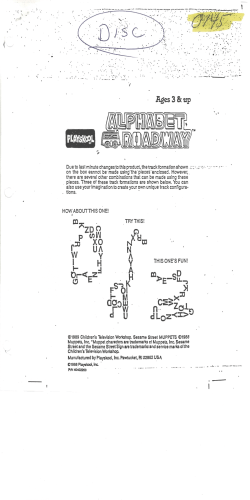
© Copyright 2026