1. No category

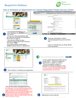
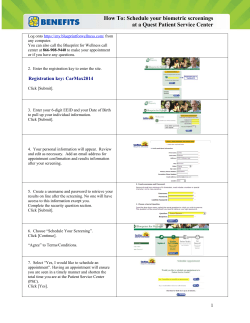
Columbia International Publishing
Journal of Healthcare Technology and Management
(2015) Vol. 3 No. 1 pp. 1-19
doi:10.7726/jhtm.2015.1001
Research Article
Genetic Algorithm–Based Outpatient Appointment
Scheduling Systems
Song Chew1* and Clariecia Groves1
Received 31 December 2014; Published online 25 April 2015
© The author(s) 2015. Published with open access at www.uscip.us
Abstract
Outpatient appointment scheduling for a clinic is a problem of assigning appointment times to patients that
seek non-emergency medical attention. This paper employs genetic algorithms to find optimal or near
optimal numbers of advanced appointment and walk-in patients to assign to each time block for a day. To this
end, an outpatient appointment schedule is represented by a vector in which a component indicates the
number of patients to be assigned to the corresponding time block. The goal is to maximize profit for the
clinic subject to such factors as the number of time blocks for a day, no-show rates, mean service times, unit
revenues, patient wait time unit cost, staff idle time unit costs, and staff overtime unit costs. Our results reveal
that all factors are influential in maximizing the profit except the staff overtime unit costs.
Keywords: Healthcare; Outpatient Appointment; Scheduling; Genetic Algorithms; Search Heuristics;
Simulation; Optimization; Operations Research
1. Introduction
Healthcare currently consumes 17% of the U.S. Gross Domestic Product and is expected to reach
20% within the coming decade (National Health Care Expenditures Projections: 2009-2019). Thus,
there is an urgent need to provide more efficient and effective patient care. The need to produce
more of a higher quality product or service at a reduced cost can only be met through better
utilization of resources (Hays and McLaughlin, 2008).
One aspect of reducing cost and improving quality of service is through outpatient appointment
scheduling. Clinical operations are driven by the patient schedule, which determines the arrival
time of patients to the clinic. Patient scheduling affects all aspects of clinical operation and is of
primary interest in any effort to improve clinic operations (Muthuraman and Lawley, 2008).
______________________________________________________________________________________________________________________________
*Corresponding e-mail: [email protected]
1 Department of Mathematics and Statistics, College of Arts and Sciences, Southern Illinois University
Edwardsville, Edwardsville, IL 62026, USA
1
Song Chew and Clariecia Groves / Journal of Healthcare Technology and Management
(2015) Vol. 3 No. 1 pp. 1-19
Effective scheduling systems have the goal of matching demand with capacity so that resources are
optimally utilized and patient waiting times are minimized (Cayirli and Veral, 2003).
Generally, the process of outpatient appointment scheduling is as follows: A patient calls for an
appointment. Next, the appointment scheduler checks for availability of the physician and/or staff
and searches for open appointment slots, which is communicated to the patient. The patient then
decides which appointment time they want and confirms the time with the scheduler before the call
ends (Muthuraman and Lawley, 2008).
A major problem in outpatient appointment scheduling is no-shows; that is, patients not showing
up for scheduled appointments. No-show rate may be considered as the probability that a patient
may not show up for a scheduled appointment. No-show rates can be as high as 40% in some clinics
(Lee et al., 2005). No-show patients bring about great uncertainty to clinical operations and limit
accessibility to other patients with reserved appointment slots that go unused. Many factors have
been cited as reasons of patient no-show, including patient demographics, medical conditions, and
environment (Deyo and Inui, 1980). Ho and Lau’s (1992) assessment of three environmental
factors (no-show probability, variability of service times, and number of patients per day) reveals
that, among the three, no-show probability is the major one that affects performance (Cayirli and
Veral, 2003).
Another major problem in outpatient appointment scheduling is walk-ins, patients seeking medical
care but not having pre-scheduled appointments. In the U.S., many clinics are the patient’s general
practitioner, and are responsible for the patient’s total care, whether elective or emergent.
Therefore, walk-ins must be anticipated and planned for in the administration of clinical
operations. Similar to no-shows, walk-in probabilities are observed to vary across specialties
(Fetter and Thompson, 1966; Field, 1980; Shonick and Klein, 1977).
This paper incorporates no-show and walk-in probabilities in the scheduling process. Specifically,
we present genetic algorithm–based outpatient appointment scheduling systems that can be used
to minimize patient waiting times, doctor and staff idle times, and doctor and staff overtime while
maximizing profit.
2. Statement of Problem
Outpatient appointment scheduling for a clinic is a problem of assigning appointment times to
patients that seek non-emergency medical attention (Chew, 2011). The goal is to assign
appointment times so that patient waiting times, doctor and staff idle time, and doctor and staff
overtime are minimized while the quality of service and revenue for the clinic is maximized.
Generally, patients that seek non-emergency medical attention can be broken down into two
categories: (1) Advanced appointment patients, and (2) walk-in patients. Advanced appointment
patients are patients that have pre-scheduled appointments; walk-in patients are patients that do
not have pre-scheduled appointments. We denote the numbers of allowed advanced appointment
(AA) patients and of allowed walk-in (WI) patients in a given day, respectively, by M and N.
2
Song Chew and Clariecia Groves / Journal of Healthcare Technology and Management
(2015) Vol. 3 No. 1 pp. 1-19
An outpatient clinic typically runs on a block schedule for each day (Chew, 2011). A day of
operations may last, say, 8 hours. Figure 1 illustrates a generic block schedule. For a given day, the
schedule may be divided into b blocks that are of an equal time interval. We call this time interval
an interappointment time, denoted by a i , i = 1, 2,…, b. Each block Bi (i = 1, 2,…, b) contains
numbers of scheduled AA and of scheduled WI patients, denoted respectively by mi and ni (i = 1,
2,…, b). Therefore, we have that M 
b
b
i 1
i 1
 mi and N   ni . We assumed that patients arrive on
time for their appointment. The arrival time of a patient, ti (i = 1, 2,…, b), is the scheduled
appointment time for the patient. Each patient is provided service for a random length of time. This
random length of time is what we refer to as service time, which we assume to be exponential. The
end time of a day is denoted by tb 1 .
B2
B1
Bb−1
Bb
m1, n1
m2, n2
m3, n3
mb−1, nb−1
mb, nb
t1
t2
t3
tb−1
tb
a1
a2
ab1
tb+1
ab
Fig. 1. An outpatient appointment schedule with b blocks.
Ideally, doctors would see each scheduled patient in block Bi during the inter-appointment time a i ,
without overlapping into the next block Bi 1 . However, many times doctors and the staff
experience idle time and/or overtime and patients experience waiting time. Idle time occurs when
the service time of patients in a block ( Bi ) ends before the scheduled arrival of patients (at time
ti+1) in the next block ( Bi 1 ). Overtime occurs when patients are still being serviced after the end (at
time tb+1) of the last block ( Bb ). Patient waiting time occurs when the patient has to wait until the
preceding patient finishes. Doctor and staff idle time, doctor and staff overtime, and patient waiting
times are considered when creating an outpatient schedule. The best and most efficient way of
dealing with these issues is to assign a unit cost to each of these factors, and then maximize the
profit (Chew, 2011). We will now refer to doctor and staff idle time, doctor and staff overtime, and
patient waiting time as cost factors. The calculation for profit will be discussed in the next section.
In addition to considering cost factors, there are other factors that will need to be considered in
order to analyze the profit. Amongst them are the following: Unit revenue (will be discussed in the
next section), no-show rates, service times, and the number of blocks. These factors will be
explored and analyzed in Sections 7 and 8.
3
Song Chew and Clariecia Groves / Journal of Healthcare Technology and Management
(2015) Vol. 3 No. 1 pp. 1-19
Our goal is to determine the optimal numbers of AA and of WI patients to assign to each block Bi
for a day so as to maximize the profit for the clinic. Furthermore, we want to determine which
factors have the greatest effect on the profit.
The remainder of the paper is organized as follows. Section 3 discusses revenues, costs, and profits
for the clinic. Section 4 talks briefly about genetic algorithms, while Section 5 expounds the way we
leverage genetic algorithms to solve our problems. Section 6 deals with confidence intervals for
profits. Section 7 presents numerical examples, and Section 8 examines the effects of factors
influencing outpatient appointment scheduling. Finally, we offer some concluding remarks in
Section 9.
3. Revenue, Expected Total Cost, and Profit
Since our main goal is to maximize the profit, we need to discuss how profit is calculated. The
general formula for profit is Profit = Revenue – Cost. The total cost C is a random variable and is
defined as follows:
C = cwW + cdD + cvV,
(1)
where W, D, and V are random variables that represent total patient waiting time, total doctor and
staff idle time and total doctor and staff overtime, respectively; and cw, cd and cv are the respective
unit costs. The values for cw, cd and cv are predetermined and are set by the clinic. We will discuss
how to calculate W, D, and V shortly.
By taking the expectation of total cost in Equation (1), we derive the expected total cost
E(C) = cwE(W) + cdE(D) + cvE(V),
(2)
where E(W), E(D) and E(V) are expected total patient waiting time, expected total doctor and staff
idle time and expected total doctor and staff overtime, respectively.
Let us discuss a few important details that will help us calculate E(W), E(D) and E(V). Let j denote a
patient and assume that each patient arrives promptly at their appointment time, tj. Now let bj, sj,
and ej, respectively, be the time at which service starts, the length of service time, and the time at
which service ends for patient j. Let us assume that the first patient’s appointment time and service
start time to be 0; that is, t1 = b1 = 0. Each patient j after the first (j > 1) will have a service start time
that is the maximum of their appointment time and the service end time of the previous patient.
Therefore, we have bj = max(tj, ej–1) and ej = bj + sj (Ho and Lau, 1992).
We can find the waiting time of patient j, wj, by considering the patient’s service start time bj minus
the patient’s appointment time tj; hence, wj = bj – tj, where w1 = 0 (Ho and Lau, 1992).
The doctor and staff are considered idle while waiting for the next patient to arrive after servicing a
patient. Thus, the doctor and staff idle time (denoted by dj) before servicing patient j is
d j  max( 0, t j  ej1 ) where d1 = 0 (Ho and Lau, 1992).
4
Song Chew and Clariecia Groves / Journal of Healthcare Technology and Management
(2015) Vol. 3 No. 1 pp. 1-19
Let T be the total number of patients scheduled for a day. In our case, T = M + N (the total number of
AA and WI patients). Further let TA = MA + NA be the total number of patients actually showing up at
the clinic for the day, where MA and NA are the numbers of AA and of WI patients actually showing
up respectively. Then the total patient waiting time and the total doctor and staff idle time are
TA
TA
j1
j1
W   wj , and D   d j , respectively. We now define the doctor and staff overtime; it is the
amount of time the doctor and staff spend providing service after the end of a day; so, the overtime
is V = max(0, eT – tb 1 ) (Ho and Lau, 1992). Note that eT is the end time of the last patient (patient
T), and that tb 1 is the end time of a day.
As mentioned earlier, service times are assumed to be random. So W, D, and V are also random. We
use E(W), E(D), and E(V) to denote the expectation of the total patient waiting time, the total doctor
and staff idle time, and the total doctor and staff overtime, respectively. We will use the averages of
h observations (or replications) of W, D, and V to approximate the respective expectations. Thus,
the expected total cost of (2) is estimated by the following average total cost
C = cw W + cd D + cv V ,
h
(3)
h
h
Wk , D  1  Dk , and V  1 Vk with Wk, Dk, and Vk being the kth observation
h k 1
h k 1
h
k 1
where W  1
of W, D, and V, respectively. This implies that E (C )  C , E ( D)  D , E (W )  W , and E (V )  V .
There will be unit revenue associated with the two types of patients, AA and WI. These associated
amounts will be denoted by r1 and r2 for AA and WI, respectively. Thus, we have that the profit P is
a random variable that can be defined as follows:
P  r1MA  r2 NA  C ,
(4)
where r1MA + r2NA is the total revenue and C is the total cost as defined by Equation (1). By taking
the expectation of the profit P, we obtain
E( P)  r1MA  r2 NA  E(C ) .
(5)
We will estimate the expected profit by the sample mean profit, P , which will be discussed in
Section 6.
Since our goal is to maximize profit, we need to determine the optimal numbers of AA and of WI
patients scheduled for each block Bi , denoted by mi* and ni* respectively, giving rise to the optimal
total numbers of AA and of WI patients, M * 
b
b
 mi* and N *   ni* respectively, and hence the
i 1
i 1


optimal total number of patients scheduled for a day, T  M  N  . Then, let M A* and N A* be the
actual numbers of AA and of WI patients, respectively, that show up in the clinic. Thus, the optimal
(maximum) profit and its expectation are respectively as follows:
5
Song Chew and Clariecia Groves / Journal of Healthcare Technology and Management
(2015) Vol. 3 No. 1 pp. 1-19
P   r1M A*  r2 N A*  C ,
E(P )  r1 M A*  r2 NA*  E(C) .
(6)
4. Genetic Algorithms
We employ genetic algorithms to find optimal or near optimal solutions. Genetic algorithms are a
search heuristic that mimics the process of evolution; a detailed introduction may be found in the
paper by Holland (1975). Most briefly, the search begins with an initial population of parent
chromosomes (often represented by vectors) randomly chosen or pre-determined. Then crossover
and mutation occur to create offspring from the parent chromosomes. There are several ways to
perform crossover. For example, during single-point crossover, one crossover point is randomly
chosen so that offspring is formed by copying the first part of a parent up to the crossover point and
last part of a second parent from the crossover point to the end. To illustrate, suppose that there are
two sequences of numbers 1, 2, 3, 4 and 5, 6, 7, 8 that are the parent chromosomes and that
point three (between the third and fourth components) is randomly chosen as the crossover point.
Then the two new offspring may be 1, 2, 3, 8 and 5, 6, 7, 4. Another way of carrying out crossover
is what is called two-point crossover. During two-point crossover, two crossover points are
randomly selected and offspring is formed from copying the first part to the first crossover point
and from the second crossover point to the end of a parent and from the first crossover point to the
second crossover point in a second parent. As an example, beginning with 1, 2, 3, 4 and 5, 6, 7, 8
as our parent chromosomes; suppose that points one and two were randomly chosen. Then two
offspring may be 1, 6, 3, 4 and 5, 2, 7, 8. Yet another way is uniform crossover. During uniform
crossover, components are randomly copied from a first parent chromosome or a second parent.
For example, beginning with 1, 2, 3, 4 and 5, 6, 7, 8, two offspring may be 1, 6, 3, 8 and 5, 2, 7,
4 such that the random crossover components are the second and fourth.
On the other hand, mutation occurs when one part of an offspring chromosome is changed.
Consider, for example, the two offspring derived in the discussion of two-point crossover, 1, 6, 3, 4
and 5, 2, 7, 8, one of them may mutate. Suppose that the third point of 1, 6, 3, 4 is mutated by
adding 1 or subtracting 1, which is equally likely to occur. As a result, the mutated offspring may
become 1, 6, 4, 4 if 1 is added, or 1, 6, 2, 4 if 1 is subtracted. After crossover and mutation, a new
population of chromosomes may be selected from the original parent and new offspring
chromosomes according to certain rules. Genetic algorithms will then repeat the above crossover
and mutation operations with the new population of (parent) chromosomes until certain criteria
are met. The stopping criterion for our genetic algorithms is that it ends when the specified number
of generations has been reached.
Genetic algorithms as a methodology have been widely employed to find optimal solutions to
optimization problem in many fields. For example, Werner (2013) provides a comprehensive
survey of genetic algorithms used for job shop scheduling problems. Genetic algorithms are also
commonly leveraged to solve production and transportation scheduling problems; for instance, see
the work by Delavar et al. (2010) for details. In the meantime, computer sciences and engineering
applications see a heavy use of genetic algorithms as well; Sharma et al. (2013) conduct a survey on
computer software testing using genetic algorithms, while Akachukwu et al. (2014) carry out a
survey of applications of genetic algorithms in engineering fields. Although they have been widely
6
Song Chew and Clariecia Groves / Journal of Healthcare Technology and Management
(2015) Vol. 3 No. 1 pp. 1-19
applied elsewhere, genetic algorithms have seen little application in the field of outpatient
appointment scheduling. Our work employing genetic algorithms seeks to fill the gap. The next
section will explain in further details how our genetic algorithms work.
5. Genetic Algorithm-Based Outpatient Appointment
Scheduling
Genetic algorithms are used to find optimal or near optimal solutions to varied types of problems.
In our case, we want to find the optimal or near optimal numbers of AA and of WI patients to assign
to each block in a day. Next, we explain the step-by-step procedure of the genetic algorithm used to
solve our problems.
Step-by-Step procedure of the genetic algorithm
Step 1:
The following parameters are predetermined:
a. number of blocks
b. interappointment time
c. number of types of patients (AA, WI, etc.)
d. no-show rate for each type of patient
e. mean service time for each type of patient, which is assumed to be exponential
f.
unit revenue for each type of patient
g. patient wait time unit cost for each type of patient
h. doctor and staff idle time unit cost for each type of patient
i.
doctor and staff overtime unit cost for each type of patient
j.
mutation rate (u %)
Step 2: An initial population of 10 (parent) schedules are randomly generated. For example, a
schedule with 8 blocks and 2 types (AA and WI) of patients is generated as follows
m1, n1; m2, n2; m3, n3; m4, n4; m5, n5; m6, n6; m7, n7; m8, n8
(7)
where mi and ni are uniform random integers from 0 to 20.
Step 3: 5 pairs of (parent) schedules are randomly chosen from the population. Then single-point
crossover occurs so that 10 offspring schedules are generated. The crossover point is randomly
chosen; so for the example in Step 2, the crossover point can be any point between any pair of
consecutive components in (7).
Step 4: Of the 10 offspring schedules, u % (we choose 70%) will be randomly chosen to be mutated.
The mutation will be performed on a randomly chosen component in each chosen schedule so that
1 will be added to or subtracted from that point, which is equally likely to occur. After the mutation
takes place on the u % of the offspring, we will then have a total of 20 schedules (10 parents and 10
offspring).
Step 5: For each of the 20 schedules, an arrangement of AA patients followed by WI patients in each
block is setup (the idea is that AA patients have higher priority over WI patients). Next, the
respective no-show rate is used to determine whether each patient in each block shows up or not. If
a patient does not show up, the patient will be removed from the schedule.
7
Song Chew and Clariecia Groves / Journal of Healthcare Technology and Management
(2015) Vol. 3 No. 1 pp. 1-19
Step 6: For each of the 20 schedules, a random service time for each patient is generated and the
profit is accordingly computed. This process is repeated multiple times; for example, we choose
3,000 times. Finally, the average of the multiple profits is computed and is designated as the
average profit for that schedule. In addition, the half-width of the 95% confidence interval for the
average profit is also computed for that schedule. This will help us determine the statistical
significance of the differences between average profits.
Step 7: The 20 schedules are ranked from the highest average profit to lowest average profit.
Step 8: The best few schedules will be chosen out of the 20 schedules and other schedules will be
randomly chosen from the remaining schedules to form a new population for the next generation.
As an example, the best schedule may be chosen and 9 others may be chosen randomly from the
remaining 19 schedules to form a new population of 10 schedules.
Step 9: Repeat Steps 3 through 8 with the new population until a pre-specified number of
generations (we choose 5,000) is reached.
6. Confidence Intervals for Profits
We discussed how profit is calculated for each schedule in Section 3. Now we discuss how
confidence intervals for profits are calculated. Before we begin, let us state the following Central
Limit Theorem:
Central Limit Theorem
If X1,…, Xn is a random sample from a distribution with mean  and variance  2   , then the
n
limiting distribution of Z n 
X
i 1
i
 n
is the standard normal; that is, Z n  Z ~ N (0,1) as
d
n
n   . Zn can also be written in relation to the sample mean as follows: Z n 
X 
/ n
.
Assume that the profit of a schedule is distributed with a mean  and variance  2   . Then by
the Central Limit Theorem, the 95% confidence interval (CI) from the mean profit is calculated as
follows:
P  1.96

h
,
(8)
where P is the sample mean profit as described by Equation (12),  is the standard deviation of
the profit P (Equation 4) and h (sample size) is a sufficiently large number of replications used to
obtain the sample mean profit. Note that we approximate  using s, the sample standard deviation
calculated by Equation (14). Therefore, Equation (8) becomes
8
Song Chew and Clariecia Groves / Journal of Healthcare Technology and Management
(2015) Vol. 3 No. 1 pp. 1-19
s
.
h
P  1.96
(9)
A single observation of the profit of a schedule is as follows:
Pk  r1M A*  r2 N A*  Ck ,
(10)
where M A* , N A* , r1 , and r2 are as defined in Section 3; Ck is a single observation of the total cost
calculated below by Equation (11):
Ck  cwWk  cd Dk  cvVk ,
(11)
where cw , cd , cv are as defined in Section 3, Wk , Dk and Vk are patient wait time, doctor and staff
idle time, and doctor and staff overtime respectively; and k = 1, 2,…, h. The sample mean profit, P , is
then calculated as follows:
P1
h
h
 Pk .
(12)
k 1
The sample standard deviation, s, is calculated as follows:
h
s2 
 (P  P )
k 1
2
k
,
h 1
(13)
so by taking the square root of both sides, we have that
h
s
 (P  P )
k 1
2
k
h 1
.
(14)
We use the sample standard deviation s instead of the actual standard deviation  because we do
not know the true standard deviation of the profits of a schedule. We use the sample variance s2 to
2
estimate the variance  and use the sample mean profit P to estimate the mean  .
7. Numerical Examples and Discussion
In this section, we discuss several examples that illustrate how the genetic algorithm can be used.
We explore and analyze the effects of multiple factors on the profit. Particularly, we look at the
effects of using various no-show rates, service times, and the numbers of blocks. For all of the
examples shown in this section, a day is 240 minutes (or 4 hours) in length. Also, staff will be
understood to include doctor(s) and the medical staff for the remainder of this paper. For each
9
Song Chew and Clariecia Groves / Journal of Healthcare Technology and Management
(2015) Vol. 3 No. 1 pp. 1-19
scenario, T1 = Patient Type 1 and T2 = Patient Type 2. In our case, T1 = AA patients and T2 = WI
patients. All simulations are programmed using MATLAB.
Example 1: No-show Rates
Since research has shown that no-show rates are a major problem for outpatient appointment
scheduling, one could analyze the impact that high no-show rates have on profit and how to
schedule patients when certain types of patients have a high probability of not showing up.
As mentioned in Section 2, walk-in patients do not have a pre-scheduled appointment. So for WI
patients, the no-show rate represents the probability of not having a patient walking in for service.
It does not represent the probability of missing an appointment.
Description
Low
Medium
High
Number of Blocks
8
8
8
Interappointment Time (minutes)
30
30
30
T1 No-show Rate (%)
10
30
70
T2 No-show Rate (%)
20
40
80
T1 Mean Service Time (minutes)
10
10
10
T2 Mean Service Time (minutes)
10
10
10
T1 Unit Revenue
300
300
300
T2 Unit Revenue
300
300
300
Wait Time Unit Cost
10
10
10
Staff Idle Time Unit Cost
5
5
5
Staff Overtime Unit Cost
5
5
5
Number of T1 Patients Scheduled
15
16
37
Number of T2 Patients Scheduled
3
7
18
Total Number of Scheduled Patients
18
23
55
2,793.8518
2,475.8363
2,007.2927
38.0925
40.8016
49.0000
Profit
Half-Width of 95% CI
Fig. 2. Scenarios with Low, Medium, and High no-show rates.
Consider that no-show rates range from 0% to 100%. Let us divide these probabilities into 3
groups: Low (between 0% and 30%), Medium (between 30% and 60%), and High (between 60%
and 100%). We will assign all patient types the same mean service time, unit revenue, and unit
10
Song Chew and Clariecia Groves / Journal of Healthcare Technology and Management
(2015) Vol. 3 No. 1 pp. 1-19
costs in order to analyze the single effect of no-show rates on the profit. Three scenarios with Low,
Medium, and High no-show rates are as indicated in Figure 2 above.
Note that for each scenario, the half-width of the 95% confidence interval (CI) is calculated for the
computed profit. The optimal schedule for each scenario is as follows in Figure 3.
Scenario
Optimal Schedule
Low
1, 2; 2, 0; 2, 0; 2, 0; 2, 0; 2, 0; 2, 0; 2, 1
Medium
3, 0; 1, 2; 1, 2; 2, 0; 2, 0; 2, 1; 3, 0; 2, 2
High
5, 3; 5, 0; 5, 0; 4, 3; 6, 0; 5, 1; 3, 3; 4, 8
Fig. 3. Optimal schedules for scenarios with Low, Medium, and High no-show rates.
A graph of the relationship between the profit (vertical axis) and the no-show rates (horizontal
axis) is shown below in Figure 4 for the 3 scenarios:
Effect of No-show Rates on Profit
3000
2500
2,794
2,476
2,007
Profit
2000
Low
1500
Medium
High
1000
500
0
Fig. 4. Effect of no-show rates on the profit.
As can be seen in the graph in Figure 4, it appears that the profit will be lower when patients have
high no-show rates.
We note that our goal is to find the optimal total numbers of patients and the corresponding
optimal distribution of these patients in each block so as to maximize the profit for the day. For
example, to maximize the profit in the Low scenario, Figures 2, 3, and 4 reveal that the optimal total
number of patients should be scheduled is 18 (15 T1 patients and 3 T2 patients), that the
11
Song Chew and Clariecia Groves / Journal of Healthcare Technology and Management
(2015) Vol. 3 No. 1 pp. 1-19
corresponding optimal distribution of these patients is 1, 2; 2, 0; 2, 0; 2, 0; 2, 0; 2, 0; 2, 0; 2, 1, and
that the optimal profit for the day is 2794. We would also like to note that if we schedule a total of
17 or 19 (simply a number other than 18 for that matter) patients, then it is possible to find the
optimal distribution of the patients and the associated optimal profit for the pre-specified number.
However, this associated profit would be less than 2794. Observe that the optimal total number of
patients scheduled will be higher when no-show rates are high. To see this, in Figure 2, notice that
the optimal total number of patients scheduled increases across scenarios (from Low to High) as
the no-show rates increase. This happens because more patients need to be scheduled in order to
account for the patients that do not show up. Scheduling more patients (or overbooking) allows the
clinic to earn a higher profit compared to not scheduling more patients when no-show rates are
high. We would like to point out that scheduling more patients to account for the possible loss of
profit does not necessarily make up the entire loss. We conjecture that high no-show rates decrease
average profit because the probability of having an optimal schedule for a day will be smaller.
Example 2: Service Times
Description
Low
Medium
High
Number of Blocks
8
8
8
Interappointment Time (minutes)
30
30
30
T1 No-show Rate (%)
10
10
10
T2 No-show Rate (%)
10
10
10
T1 Mean Service Time (minutes)
10
30
70
T2 Mean Service Time (minutes)
20
40
80
T1 Unit Revenue
200
200
200
T2 Unit Revenue
200
200
200
Wait Time Unit Cost
10
10
10
Staff Idle Time Unit Cost
10
10
10
Staff Overtime Unit Cost
5
5
5
Number of T1 Patients Scheduled
15
6
1
Number of T2 Patients Scheduled
1
0
1
Total Number of Scheduled Patients
16
6
2
Profit
748.4459
‒615.4773
‒1,106.3145
Half-Width of 95% CI
30.2537
31.2649
23.5858
Fig. 5. Scenarios with Low, Medium, and High service times.
12
Song Chew and Clariecia Groves / Journal of Healthcare Technology and Management
(2015) Vol. 3 No. 1 pp. 1-19
Service times may have significant effects on scheduling and profit. We will illustrate through a few
examples some of the possible effects of various mean service times. Consider that service times are
exponentially distributed (chosen for convenience; any type of distribution may be used). Let us
divide the range of all possible values of the mean service time into 3 groups: Low (between 0 and
30 minutes), Medium (between 30 and 60 minutes), and High (greater than 60 minutes). We will
assign all patient types the same no-show rate, unit revenue, and unit costs in order to analyze the
effect of service times on the profit. Three scenarios with Low, Medium, and High mean service
times are as indicated in Figure 5.
Observe that the optimal total number of patients scheduled will be smaller when the mean service
times are high. For example, notice, in Figure 5, that the optimal total number of patients scheduled
decreases across scenarios (from Low to High) as the mean service times increase. This occurs
because longer service times allow less time to service more patients. The optimal schedule for
each scenario is provided in Figure 6.
Scenario
Optimal Schedule
Low
2, 0; 2, 0; 2, 0; 2, 0; 2, 0; 2, 0; 2, 0; 1, 1
Medium
1, 0; 1, 0; 0, 0; 1, 0; 1, 0; 0, 0; 1, 0; 1, 0
High
1, 0; 0, 0; 0, 0; 0, 1; 0, 0; 0, 0; 0, 0; 0, 0
Fig. 6. Optimal schedules for scenarios with Low, Medium, and High service times.
A graph of the relationship between profit (vertical axis) and the mean service times (horizontal
axis) is shown in Figure 7 for the 3 scenarios.
Fig. 7. Effect of mean service times on profit.
13
Song Chew and Clariecia Groves / Journal of Healthcare Technology and Management
(2015) Vol. 3 No. 1 pp. 1-19
Similar to the results in Figure 4 for various no-show rates, in Figure 7, it appears that the profit
will be lower when patients have longer service times.
Example 3: Number of Blocks
If we want to determine the optimal number of blocks given a set of parameters (Step 1: b to j in
Section 5), we may run our genetic algorithm using a different number of blocks for each run while
keeping all the other parameters the same across each run. The optimal number of blocks would be
the number of blocks associated with the highest profit.
We have found the optimal number of blocks for three scenarios. For each scenario, we run the
algorithm for each of the following numbers of blocks: 4, 6, 8, 12, 16, and 24. Assuming a 4-hour
day, note that the corresponding interappointment times are 60, 40, 30, 20, 15, and 10 minutes,
respectively. Scenarios 1–3 are as indicated in Figure 8 where T1 may be AA patients and T2 may
be WI patients.
Description
Scenario 1
Scenario 2
Scenario 3
T1 No-show Rate (%)
10
20
10
T2 No-show Rate (%)
20
10
20
T1 Mean Service Time (minutes)
10
20
50
T2 Mean Service Time (minutes)
20
10
40
T1 Unit Revenue
150
300
500
T2 Unit Revenue
300
100
150
Wait Time Unit Cost
10
5
10
Staff Idle Time Unit Cost
5
20
10
Staff Overtime Unit Cost
5
10
5
Fig. 8. Parameters for 3 scenarios.
A graph of the relationship between profit (vertical axis) and the number of blocks (horizontal axis)
is shown in Figures 9, 10, and 11 below for the 3 scenarios. From the graph in Figure 9, the optimal
number of blocks appears to be 24 for Scenario 1. Figure 10 depicts that the optimal number of
blocks seems to be 16 for Scenario 2, while Figure 11 reveals that the optimal number of blocks
should be 16 for Scenario 3.
14
Song Chew and Clariecia Groves / Journal of Healthcare Technology and Management
(2015) Vol. 3 No. 1 pp. 1-19
Fig. 9. Effect of numbers of blocks on profit for Scenario 1.
Fig. 10. Effect of numbers of blocks on profit for Scenario 2.
15
Song Chew and Clariecia Groves / Journal of Healthcare Technology and Management
(2015) Vol. 3 No. 1 pp. 1-19
Fig. 11. Effect of numbers of blocks on profit for Scenario 3.
Overall, the graph of the profit generated for 4, 6, 8, 12, 16, and 24 blocks appears to be unimodal.
Thus, we conjecture that the profit function is unimodal in the number of blocks. Having this
unimodal shape is very helpful in determining the optimal number of blocks for a given set of
parameters.
Note that the total number of patients to schedule for a day changes over different numbers of
blocks. For example, Scenario 1 has the following results, as shown in Figure 12, for the total
number of patients for 4, 6, 8, 12, 16, and 24 blocks. Thus, for Scenario 1, a clinic would need to
schedule 15 patients if they employ 24 blocks compared to 8 patients for 4 blocks in order to
maximize their profit.
Number of Blocks
4
6
8
12 16 24
Total Number of Patients
8
10
10 11 12 15
Fig. 12. Total number of patients for a day for Scenario 1.
Perhaps there are other factors that affect the profit. To this end, we will conduct regression
analysis and use the results of model selection to analyze the effects of multiple factors
(independent variables) on the profit (dependent variable).
8. Model Selection
Model selection, also known as subset selection or variables selection procedures, have been
developed to identify a small group of regression models that are “good” according to a specified
16
Song Chew and Clariecia Groves / Journal of Healthcare Technology and Management
(2015) Vol. 3 No. 1 pp. 1-19
criterion (Kutner et al., 2004). The results of model selection will indicate which factors are most
important or useful in predicting profit. Thus, by using model selection, we will determine which of
the following factors (or independent variables) have the greatest effect on the profit:
1.
2.
3.
4.
5.
6.
7.
number of blocks
no-show rate
mean service time
unit revenue
wait time unit cost
staff idle time unit cost
staff overtime unit cost
While there have been many criteria used for comparing regression models, we will use the
following procedures to select the best models: Adjusted R2, Mallow’s Cp (where p – 1 is the number
of variables and p includes the intercept term), forward selection, and backward elimination. For
the forward selection and backward elimination procedures, we will use Akaike’s information
criterion (AICp). A brief description of these procedures is as follows:
Adjusted R2: This procedure is similar to using R2, the coefficient of multiple determination, except
that it takes the number of variables in the regression model into account through the degrees of
freedom (Kutner et al., 2004). The best model will have the largest value. Here is the formula:
 n  1  SSE p

Ra2, p  1  
, where SSEp is the error sum of squares and SSTO is the total sum of
 n  p  SSTO
squares.
Mallow’s Cp: This procedure uses the total mean squared error of the fitted values for each subset
regression model to rank the models (Kutner et al., 2004). The best model will have the smallest
value. Here is the formula: C p 
SSE p
MSE ( X 1 ,..., X p 1 )
 (n  2 p) , where MSE is the error mean
square.
AICp: This procedure uses the natural log of the error of sum of squares to rank the models (Kutner
et al., 2004). The best model will have the smallest value. Here is the formula:
AIC p  n ln SSE p  n ln n  2 p .
Forward Selection: This procedure begins with no independent variables. At each step, it adds the
variable that (after being added) will give the lowest value of the AICp statistic. The procedure will
stop at the step where adding a variable would increase the AICp statistic. Thus, the procedure will
not add the variable that would increase the AICp statistic and the best model will be the resulting
model after the procedure ends.
Backward Elimination: This procedure begins with all independent variables included. At each
step, it removes the variable that (after being removed) will give the lowest value of the AICp
statistic. The procedure will stop at the step where removing a variable would increase the AIC p
17
Song Chew and Clariecia Groves / Journal of Healthcare Technology and Management
(2015) Vol. 3 No. 1 pp. 1-19
statistic. Thus, the procedure will not remove the variable that would increase the AIC p statistic and
the best model will be the resulting model after the procedure ends.
Here are the results of model selection. Using Adjusted R2, the best model included all factors
except staff overtime unit cost. The value of Adjusted R2 for the best model was 0.8664862. Using
Mallow’s Cp, the best model included all factors except staff overtime unit cost. The value of
Mallow’s Cp was 6.867845. Using forward selection (with AICp), the best model included all factors
except staff overtime unit cost. The value of AICp was 1622.06. Using backward elimination (with
AICp), the best model included all factors except staff overtime unit cost. The value of AICp was
1622.06.
Since all procedures returned the same subset of independent variables, we conclude that the
factors that have the greatest effect on the profit function are the following: number of blocks, noshow rate, mean service time, unit revenue, wait time unit cost, and staff idle time unit cost.
To further validate our conclusion, we should check for multicollinearity. Multicollinearity is a
statistical phenomenon in which two or more independent variables in a multiple regression model
are highly correlated. When this occurs, some of the independent variables may be redundant in the
model because of their correlation with other variables. To check for multicollinearity, we
computed the correlation between pairs of independent variables and found that there was no
correlation between all pairs of independent variables. Thus, this provides strong evidence that
there is no issue of multicollinearity and we may conclude that all factors except staff overtime unit
cost can be used to analyze the profit function.
9. Conclusion
In this project, the objective was to find the optimal number of patients to schedule for each block
and for each type of patient (typically advanced appointment and walk-in patients) along with the
optimal profit given a set of parameters. We used genetic algorithms in order to find an optimal or
near optimal solution to this scheduling problem. Through multiple experiments of running
simulations along with using model selection, we were able to draw conclusions about the effects of
number of blocks, no-show rates, mean service times, unit revenue, and unit costs on the profit. In
addition, we were able to employ genetic algorithms to find the optimal or near optimal number of
patients (of each patient type) to schedule for each block.
References
Akachukwu, C., Aibinu, A., Nwohu, M., & Salau, H. (2014). A decade survey of engineering applications of
Akachukwu, C., Aibinu, A., Nwohu, M., & Salau, H. (2014). A decade survey of engineering applications of
genetic algorithm in power system optimization. In Fifth international conference on intelligent systems,
modelling and simulation (pp. 38-42).
Cayirli, T., & Veral, E. (2003). Outpatient scheduling in health care: A review of literature. Production and
Operations Management, 2(4), 519-549.
http://dx.doi.org/10.1111/j.1937-5956.2003.tb00218.x
Chew, S. (2011). Outpatient appointment scheduling with variable interappointment times. Journal of
Modelling and Simulation in Engineering, 2011, 1-9.
18
Song Chew and Clariecia Groves / Journal of Healthcare Technology and Management
(2015) Vol. 3 No. 1 pp. 1-19
http://dx.doi.org/10.1155/2011/909463
Delavar, M., Hajiaghaei-Keshteli, M., & Molla-Alizadeh-Zavardehi, S. (2010). Genetic algorithms for
coordinated scheduling of production and air transportation. Expert Systems with Applications, 37, 82558266.
http://dx.doi.org/10.1016/j.eswa.2010.05.060
Deyo, A., & Inui, S. (1980). Dropouts and broken appointments. Medical Care, 18(11), 1146-1157.
http://dx.doi.org/10.1097/00005650-198011000-00006
Fetter, R., & Thompson, J. (1966). Patients' waiting time and doctors' idle time in the outpatient setting.
Health Services Research, 1, 66-90.
Field, J. (1980). Problems of urgent consultations within and appointment system. Journal of the Royal College
General Practitioners, 30, 173-177.
Hays, J., & McLaughlin, D. (2008). Healthcare operations management. In Foundation of the American College
of Healthcare Executives.
Ho, C., & Lau, H. (1992). Minimizing total cost in scheduling outpatient appointments. Management Science,
38(12), 1750-1764.
http://dx.doi.org/10.1287/mnsc.38.12.1750
Holland, J. (1975). Adaptation in natural and artificial Systems. Univ. Michigan, Ann Arbor, MI.
Kutner, M., Nachtsheim, C., & Neter, J. (2004). Applied Linear Regression Models. Fifth Edition, McGrawHill/Irwin. National Health Care Expenditures Projections: 2009-2019. Centers for Medicare and Office of
the Actuary Medicaid Services, USA.
Lee, J., Earnest, A., Chen, M., & Krishnan, B. (2005). Predictors of failed attendances in a multi-specialty
outpatient centre using electronic databases. BMC Health Services Research, 5(51), doi:10.1186/14726963-5-51.
http://dx.doi.org/10.1186/1472-6963-5-51
Muthuraman, K., & Lawley, M. (2008). A stochastic overbooking model for outpatient clinical scheduling with
no-shows. IIE Transactions, 40, 820-837.
http://dx.doi.org/10.1080/07408170802165823
Sharma, C., Sabharwal, S., & Sibal, R. (2013). A survey on software testing techniques using genetic algorithm.
International Journal of Computer Science Issues, 10, 381-393.
Shonick, W., & Klein, B. (1977). An approach to reducing the adverse effects of broken appointments in
primary care systems: Development of a decision rule based on estimated conditional probabilities.
Medical Care, 15(5), 419-429.
http://dx.doi.org/10.1097/00005650-197705000-00008
Werner, F. (2013). A Survey of Genetic Algorithms for Shop Scheduling Problems. Heuristics: Theory and
Applications, Nova Science Publishers, 161-222.
19