1. technology and computing
2. software

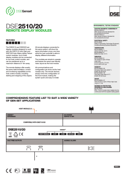
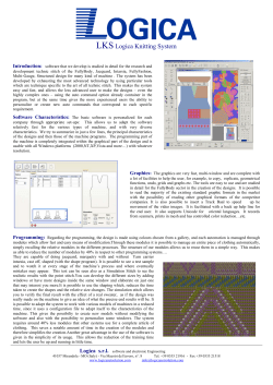
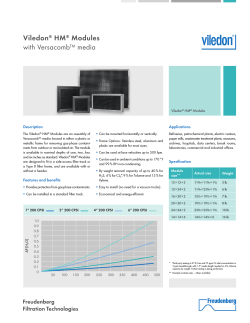
A Graph-Theoretic Method for Mining Functional
Modules in Large Sparse Protein Interaction
Networks
Shi-Hua Zhang1∗ Hong-Wei Liu2
Xue-Mei Ning1
Xiang-Sun Zhang1
1
Academy of Mathematics and Systems Science
Chinese Academy of Sciences, Beijing 100080, China
2
School of Economics, Renmin University of China, Beijing 100872, China
Abstract
With ever increasing amount of available data on protein-protein interaction (PPI) networks,
understanding the topology of the networks and then biochemical processes in cells has become a key
problem. Modular architecture which encompasses groups of genes/proteins involved in elementary
biological functional units is a basic form of the organization of interacting proteins. Here we propose
a method that combines the line graph transformation and clique percolation clustering algorithm
to detect network modules which may overlap each other in large sparse protein-protein interaction
(PPI) networks. The resulting modules by the present method show a high coverage among yeast, fly,
and worm PPI networks respectively. Our analysis of the yeast PPI network suggests that most of
these modules have well biological significance in context of protein localization, function annotation,
and protein complexes. The overlapping modules form a cartographic network representation which
also shows well scale-free property.
Key words: Protein-Protein Interaction (PPI) network, network clustering, line graph transformation, protein complexes, functional modules.
1
Introduction
Large-scale interaction detection methods have resulted in a large amount of protein-protein interaction (PPI) data. Studying the network of the interactions can help biologists to understand principles
of cellular organization and biochemical phenomena. Functional modules as a critical level of biological hierarchy and relatively independent units play a special role in biological networks [1]. Since
network modules do not occur by chance [2], identification of modules is likely to capture the biologically meaningful interactions. Naturally, revealing modular structures in biological networks is a
preliminary step for understanding how cells function and how proteins organize into a system.
Many methods based on modeling the PPI data with a graph have been developed for analyzing
the network structure of PPI networks. Hierarchical clustering methods have been proven to be a
good strategy for metabolic networks and PPI networks. Ravasz et al. [3] analyzed the hierarchical
organization of modularity in metabolic networks, and authors of [4–6] applied three different clustering methods respectively, based on different metrics induced by shortest-distance, graphical distances,
and probabilistic functions, to analyze the module structure of the yeast protein interaction networks
on a clustering tree. Several papers [2, 7, 8] have also shown that network modules which are densely
connected within themselves but sparsely connected with the rest of network generally correspond to
meaningful biological units such as protein complexes and functional modules. Bu et al. [8] found 48
functional modules in budding yeast by applying a spectral analysis method. Prediction methods of
protein complexes which generally correspond to dense subgraphs in the network have been proposed
by [2, 7, 9]. Several approaches to network clustering that have been used for analyzing PPI networks
∗ Corresponding
author. Fax: +86-10-62561963. E-mail address: [email protected]
1
include edge-betweenness clustering [10], identification of k-cores [7], restricted neighborhood search
clustering (RNSC) [9] and Markov clustering algorithm (MCL) [11]. Spirin and Mirny [2] detected
about 50 network modules by using a combination of three methods (enumeration of complete subgraphs, superparamagnetic clustering and Monte Carlo simulation), and most of which have been
proven to be protein complexes or functional modules.
There are two problems to be concerned. Most current methods are partition algorithms which
mean that each protein belongs to only one specific module. Such algorithms are not suitable for
finding overlapping modules. Another problem is that PPI networks are very sparse, while most
methods only identify strongly connected subgraphs as modules, so only a few modules were detected
such as in [7, 9].
Recently, a novel network clustering method (Clique Percolation Method, CPM) based on clique
percolation has been developed [12]. It can reveal overlapping module structure of complex networks.
But a distinct shortcoming of its application in PPI networks lies in that the method may be restrictive
since the basal element of the method is a 3-clique structure. For example, the spoken-like module
can not be detected and when the method is applied to large sparse PPI networks such as fly and
worm PPI networks, only a few modules can be detected. In order to overcome the problem, line
graph transformation (LGT), an important graph-theoretical technique was introduced here. Some
studies about the line graph transformation related with biological networks have been done. Two
papers [13, 14] had made detailed analysis of the line graph transformation focused on the degree
distribution P (k) and degree-dependent clustering coefficient C(k) respectively. We show that the
combined method (LGT-CPM) of LGT and CPM possesses very distinguished merit and the modules
detected by the present method carry distinguished biological significance. We also make a comparison
of our method with other network clustering methods such as restricted neighborhood search clustering
(RNSC) [9] to verify its effectiveness.
2
2.1
Materials and Methods
Materials
Large-scale protein interaction datasets for S.cerevisiae, D.melanogaster, C.elegans, are used in this
study. Pre-processed interaction data for yeast Sacchromyces cerevisiae is obtained from [6] where the
data is further collected from the MIPS (http://mips.gsf.de/), PreBIND (http://www.blueprint.org
/products/prebind/index.html), BIND (http:// bind.ca/), GRID (http://biodata.mshri.on.ca/grid/
servlet/Index) and the spoke model data [15]. Fly and worm PPI datasets are obtained from [16, 17]
respectively. After pre-processing (removing self-interactions and repeated interactions), the information of the three protein interaction networks can be seen in Table 1. A standing functional annotation
table (funcat-2.0 data 20062005) and a list of protein complexes (complexcat data 20062005) are also
obtained from MIPS for verification and analysis. And experimental protein localization data by
Huh et al. (2003) is downloaded from the web site http://yeastgfp.ucsf.edu/. The BioLayout [18]
(http://cgg.ebi.ac.uk/services/biolayout/) program is used to view the resulting modules.
Table 1: Large scale protein interaction data used in this study.
Organism
S.cerevisiae
D.melanogaster
C.elegans
Network
Sc
Dm
Ce
No. of Proteins
4537
6984
2892
No. of Interactions
13344
20191
4622
No. of with unique interaction
1208
2292
1624
Reference
[6]
[16]
[17]
In order to extract interesting modules in PPI networks, a four-step procedure is needed. First, we
compute the line graph L(G) of the original PPI network G. Then, we apply the clique percolation
clustering method on the L(G). In the third step, the resulting modules in L(G) are transformed
back to modules in G. The final step is merging two heavily overlapped modules into one. The left
plot of Figure 1 shows the scheme of the method, while the right shows the contrast between CPM
and LGT-CPM. We can find that the present method adds more nodes into the module detected by
CPM.
2
PPI network G
Line graph transformation
L(G)
Percolation clustering
k-clique clusters in L(G)
Rediscovering in G
Overlapping modules in G
Merging
Final overlapping modules in G
Function annotation, protein
complexes
and
pathways
Functional modules
Figure 1: The left plot is the schematic diagram of LGT-CPM method for detection of network
modules and the right is the sketch map of CPM and LGT-CPM.
2.2
Clique percolation method (CPM)
Recently, a powerful tool based on clique percolation for finding modules (communities or clusters) and
exploring the general characteristics of complex networks in nature and society was developed by Palla
et al. [12]. The underlying idea of the method is the concept of k-clique community which was defined
as a union of all k-cliques (complete subgraphs of size k) that can be reached from each other through a
series of adjacent k-cliques (where adjacency means sharing k −1 nodes). The k-clique community can
be considered as a usual module because of its dense internal linkage and sparse external linkage with
other part of the whole network. The authors have analyzed the theoretical basis of applicability of
the new community definition to real network according to a sharp percolation transition phenomena
of the Erd¨os-R´enyi uncorrelated random graph, and made some preliminary experiments using some
real networks. A distinguishing feature of CPM is that it can uncover the overlapping community
structure of complex networks, i.e., one node can belong to several communities.
2.3
Line graph transformation (LGT)
Just as we have pointed that the direct application of clique percolation clustering method may be too
restrictive to detect proper modules in sparse networks. As a straightforward example, the spoken-like
modules can not be detected. Line graph transformation is a mapping that transforms a graph G into
its associated line graph L(G) by transforming nodes into edges. This simple graph operation has
outstanding advantages for graph clustering: it does not lose information because the original network
can be recovered and the transformed graph is more highly structured than the original network. So
it is much more convenient than directly using clique percolation clustering. For the sake of CPM
computation, we will extract the nodes with large degree in G so that the line graph corresponds to
a graph without cliques of very large size. After rediscovering modules, we assign these nodes to one
module or more than one modules according to its linkage with the module(s). It will enhance the
computational efficiency and consequently produce very little affect to the resulting modules.
Then, we apply the clique percolation method (CPM) to the line graph of these networks and
detect interesting modules which may overlap each other. Different k values can lead to different
k-clique communities. We analyze the PPI network with different k-clique communities on L(G).
But we only make 4-clique communities as an example of our method. These clusters (modules) of
line graph L(G) are then transformed back to protein-protein subnet of the original PPI network G.
We simply call it the reverse transformation of line graph (RLG). In detail, the edges in G which
correspond to the nodes of a module in L(G) will form a subnet of the original network G, and then
we add the lost edges within the nodes of the subnet to form modules in the original PPI network. A
3
post-processing step for merging is executed for two modules which have a large overlap.
2.4
Functional annotation, protein localization and validation of protein
complexes
In order to detect the functional characteristics of the numerically computed modules, we compared
them with known functional classification. The P -value, which is the probability that a given set
of proteins is enriched by a given functional group merely by chance, following the hypergeometric
distribution, was often used as a criteria to assign each module a main function [8, 9]. Here, we also
assign a function category to a specific module when the minimum P -value occurrs. The P -value for
a module M and function category F is defined as:
µ
¶µ
¶
|F |
N − |F |
k−1
X
i
|M | − i
µ
¶
,
P =1−
N
i=0
|M |
where module M contains k proteins in F , and the PPI network contains N proteins. The smallest
P -value over all functional categories is defined as the P -value of a module which also means that
the module is assigned the corresponding function category. In a similar way, we can also check the
module’s localization consistency using the P -value.
Modules may correspond to real protein complexes. We try to match the numerically computed
modules with the experimentally determined complexes. A best-matching criteria which was first
introduced in [2] is used here. By minimizing the probability Pol of a random overlap between a
computational group and an experimental group, we can determine the best-matching experimental
complex for a module. The Pol is defined as:
µ
¶µ
¶
|M |
N − |M |
k
|C| − k
µ
¶
Pol =
,
N
|C|
where |C|, |M | are the sizes of an experimental complex and a computed module respectively, N is
the size of the network and k is the number of their common proteins.
3
Results
We apply the present method to three PPI networks and detect interesting modules which may
overlap each other. The CFinder software (http://angel.elte.hu/clustering/) implementing CPM is
downloaded under public license and is used in our analysis. To analyze the PPI network, we apply
the clique percolation method to calculate all 4-clique communities of the line graphs of the three PPI
networks. In order to compare the LGT-CPM with CPM, we also apply CPM on these three PPI
networks (see Table 2). For instance, we obtain 1070 protein modules of sizes from 5 to 52, while only
obtain 267 and 93 modules by CPM with 3-clique communities and 5-clique communities of the yeast
PPI network with minimum size 3 and 5 respectively.
Table 2: Number of modules detected by CPM and LGT-CPM
Organism
S.cerevisiae
D.melanogaster
C.elegans
Min. size
3(5)
3(5)
3(5)
No. (CPM)
267 (93)
257 (29)
44 (10)
Coverage
27.22% (19.13%)
9.58% (2.92%)
6.36% (3.39%)
4
Min. size
5
5
5
No. (LGT-CPM)
1070
1978
408
Coverage
74.19%
78.57%
63.80%
Module localization consistency
250
Frequency
200
150
100
50
0
0
2.5
2
1.5
1
0.5
0
0.1
0.2
0.3
0.4
0.5
0.6 >0.6
Module localization consistency
10
20
30
Module size
40
50
Figure 2: Proteins within a detected module have high localization consistency. The left plot shows
the frequency of localization consistency and the right shows the scatter plot of modules’ localization
consistency and module size. The dash line indicates the total consistency averaged over all pairs of
the yeast proteins.
3.1
Proteins in the same module have the same localization
Recent studies show that a majority of interactions between proteins are in the same primary compartment (same localization) [19, 20]. Since a functional module performs a relatively independent
cellular function, the same localization is expected to appear for such a unit. We employ Huh’s protein
localization data [20] to verify this idea. After excluding proteins who are not included in our PPI
data, the dataset contains 3270 proteins which cover 23 distinct subcellular locations. We naturally
represent each protein’s localization as a binary vector of 23 dimensions in which 1 means this protein
appearing in this location, 0 otherwise. We only consider the modules whose proteins are mostly
covered by protein localization dataset. We take 700 out of 1070 functional modules as example in
which each module is covered at least 80% by the localization data.
We use the inner product of two vectors to represent the localization consistency between two
proteins, and the average consistency of all protein pairs to represent the localization consistency of a
module. Figure 2 shows the distribution of localization consistency of all the 700 functional modules.
For 480 out of 700 (68.6%), the average localization consistency is higher than the average localization
consistency over all the 3270 yeast proteins. While according to the P -value of the modules based on
localization data, 574, 386, and 304 out 700 modules have well localization consistency with P < 0.05,
P < 0.01, and P < 0.005 respectively. We also check the relationship between the module size and
localization consistency, and find no significant correlation. (see the left plot of Figure 2). All these
suggest that functional modules detected by the present method are biologically significant.
3.2
Functional annotation of network modules
The basic hypothesis is that the identified modules represent functional modules whose proteins are
involved in the same functional process or biological unit. To test this idea and annotate the computed
modules, we compare them with the functional annotation of Sacchromyces cerevisiae genes in the
MIPS Functional Catalog (FunCat) database. FunCat [21] is an annotation scheme for the functional
description of proteins having various biological functions and consists of 28 main functional categories
(in total, there are 16 main functional categories for current yeast data). We find that 577 and 496
out of 1070 modules match well with known functional categories with P < 0.01 and P < 0.005
respectively. Taking into account the incompleteness of the current function annotation data, the
remaining modules may also correspond to well functional categories. We choose 20 modules randomly
with P < 0.001 and their function categories as example (see Table 3).
Figure 3 shows the consistency instance of 805 out of 1070 modules corresponding at least one
5
Table 3: Examples: the detected modules matched with function categories which were cataloged
in MIPS. MO represents the order of module and main functional category means the functional
annotation of modules.
MO
4
62
97
Module’s proteins
YIL131C YHL027W YOR275C YJL056C YMR032W
YBR044C YKL141W YLL041C YKL148C YBR221C
YLR116W YOR142W-A YIL145C YPR158W-A YOL103W-B YKL057C
−log10(P )
3.6361
4.1154
5.0078
98
109
118
215
YLR262C YLR039C YDR137W YLR304C YER136W YMR235C
YMR043W YCL067C YCR040W YCR039C YOR088W YLR082C
YNL102W YJR043C YJR006W YDL102W YBR088C
YKL080W YBR127C YHR039C-A YGR117C YJR033C YDL185W
4.1738
4.4832
3.5953
4.8130
240
247
263
266
YDR071C YBR125C YER089C YPL153C YBL056W YDR247W
YBR102C YLR166C YIL068C YER008C YML097C YPR055W YDR166C
YOR212W YCL032W YLR362W YDR103W YDR032C YBR059C YPR076W
YLL039C YDR143C YOL094C YPR010C YLR229C YPR019W YPL113C
3.6126
5.6509
4.6912
3.4620
304
386
405
YLR006C YCR073C YDL235C YLR233C YDL013W YNR031C YMR022W
YLR208W YJL002C YMR146C YGL100W YML130C YEL002C YGL022W YML019W
YML065W YDR171W YBR060C YKR101W YNL261W YPR162C YHR118C YLL004W
7.1549
3.9859
6.9208
509
YKL080W YDR523C YNL250W YDL185W YGR020C YEL051W YHR060W YOR332W
YPR036W YHR039C-A YOR270C
YNL258C YPR105C YPR040W YMR020W YPR181C YLR268W YIL109C YPL218W
YOR075W YDR498C YDR004W YLR078C YLR026C YGL145W
YOR212W YDR103W YLR362W YBL016W YBR200W YDL159W YGR179C YER132C
YBR046C YDR264C YBR045C YCL032W
YAL035W YFR031C-A YER006W YPL093W YBR084W YDR101C YNL112W YGR204W
YPL009C YOR048C YBR263W YGL099W
YOR160W YJR132W YGR119C YJL041W YLR293C YMR024W YJL061W YFR002W
YIL115C YDR322W YDR116C YJL063C YML025C YMR193W YLR312W-A YDR395W
YGL172W
YPR088C YCL037C YNL110C YNL154C YPR137W YHR052W YIL131C YDL014W
YJL069C YER161C YDR060W YLR175W YGR274C YOL102C YGL120C YGL130W
YDL208W YKL078W YAL035W YJL033W YLR197W YOR310C YCL054W YNL230C
8.3979
646
653
669
810
886
3.7870
Main functional category
cell type differentiation
energy
transposable elements,
viral and plasmid proteins
protein activity regulation
development (systemic)
cell cycle and dna processing
interaction with the
cellular environment
metabolism
cell type differentiation
interaction with the environment
protein with binding function
or cofactor requirement
cell rescue, defense and virulence
protein fate
interaction with the
cellular environment
interaction with the
cellular environment
cellular transport, transport
facilitation and transport routes
cellular communication/signal
transduction mechanism
protein synthesis
8.6990
biogenesis of cellular components
8.3979
transcription
6.1373
6.7799
functional category with P < 0.01 versus the module size. The plot suggests that the function
homogeneity of modules does not depend on the modules’ size.
3.3
Matching with experimentally determined complexes
We match the computed modules with experimentally determined complexes using the best-matching
criteria. Comparison of the numerically computed modules with the experimentally determined complexes shows a very good agreement. The gold-standard complexes used here are those catalogued
in the MIPS database [22], in which there are 817 complexes with the size at least 3. In total 542
modules can be found matching at least one experimentally determined complex at a higher level
with log(Pol ) < −17. Figure 4 shows three examples of eligible modules of size 10, 7 and 14 which
correspond to well known complexes. The first two are both completely included in different complexes: cellular complexes (550.1.136) and Coat complexes II (260.30.20). The third one has 8 proteins
belonging to transport across the outer membrane complex (290.10) of size 9 (note that 4 out of the
14 proteins in the modules are not included in MIPS complexes data). We choose 20 modules randomly which match well with the experimentally determined protein complexes with log(Pol ) < −17
as examples (see in table 4). We also test the coverage of predicted complexes, i.e., the degree to
which entire complexes appear in the same detected modules [23]. Figure 5 shows the coverage of our
results for varying coverage ratio values. For example, there are 561/459 MIPS complexes for which
60%/80% or more of their members appeared in the same detected modules.
3.4
Comparison with related methods
Comparison with other module detecting methods is difficult because of the ambiguous definition of
a module and complexity of a network. But an obvious advantage is that the present method can
detect modules which have higher coverage ratio than general methods such as CPM, RNSC and
MCODE and the resulting modules are still of biological significance. Furthermore the new method is
automatic and deterministic, while in a related research [2], Spirin and Mirny used the combined results
of three methods (enumeration of complete subgraphs, superparamagnetic clustering and Monte Carlo
simulation) with some clearing and emerging processing to detect the modular structure of a given
6
6.0
5.5
5.0
−log10(P)
4.5
4.0
3.5
3.0
2.5
2.0
1.5
10
20
30
Module size
40
50
Figure 3: The scatter plot of P -value of modules versus module size. The dash line indicates the
P = 0.01 and P = 0.005 respectively (Note: in order to get rid of the effect of large values of
−log10(P ), we assign the −log10(P ) equal to 6 when their actual values are larger than 6).
Figure 4: Three examples of detected modules which match well with experimentally determined
protein complexes.
600
Num of complexes
500
400
300
200
100
0
50
60
70
80
Coverage ratio (%)
90
100
Figure 5: Complex coverage which represents the number of complexes whose member proteins appear
in the same predicted complex with respect to various thresholds.
7
Table 4: Examples: the detected modules match well with experimentally determined protein complexes which were cataloged in MIPS. MO represents numerically determined module, MIPS tag
represents ’complexes’ tag cataloged in MIPS and OL represents the size of overlapping.
MO
138
164
247
316
333
394
405
509
515
562
601
691
710
789
844
888
936
1005
1043
1069
MIPS tag
260.20.30
290.20.10
160
510.150
270.20.30
440.12.20
410.10
220
310.40
260.30.20
550.2.26
510.10
550.2.29
140.10.20
550.2.34
60
550.2.182
133.10
230.20.20
550.2.62
Sizes
7 ( 7)
8 (11)
7 ( 7)
7 ( 7)
6 ( 7)
8 ( 8)
8 ( 8)
11 (11)
8 (10)
7 ( 7)
11 (11)
14 (14)
12 (13)
12 (12)
15 (15)
23 (26)
18 (18)
24 (27)
25 (28)
31 (31)
4 ( 4)
5 ( 5)
7 ( 7)
5 ( 5)
7 ( 9)
8 ( 9)
6 ( 6)
13 (15)
6 ( 6)
11 (11)
11 (11)
13 (14)
13 (13)
7 ( 7)
11 (11)
11 (11)
16 (16)
10 (10)
16 (16)
26 (26)
OL
4
5
5
5
4
8
6
8
5
7
11
5
11
5
10
11
15
10
11
26
log(Pol )
-26.95
-33.29
-31.22
-34.27
-24.24
-56.75
-40.61
-44.49
-31.49
-44.61
-75.11
-22.56
-68.26
-27.59
-58.68
-60.99
-88.90
-54.60
-51.43
-145.54
PPI network. The last two methods are stochastic and rely heavily on post-processing. Restricted
neighborhood search clustering (RNSC) [9], which was used to predict protein complexes, is also a
stochastic network clustering method, so repeated runs on the same input network may result in
different clusterings.
The LGT-CPM method can also be considered as a complexes prediction system just as RNSC
and MCODE. Bader and Hougue generated a set of 209 predicted complexes, of which 54 match the
original MIPS complexes dataset. King et al. [9] applied RNSC algorithm to predict complexes from
protein interaction networks. But they only predicted 45 complexes which match 30 MIPS complexes
in yeast. And they only detected 5 and 45 modules in worm and fly PPI networks respectively.
Obviously, our approach predicted more modules than other methods. Since the known complex set
is heavily incomplete, some yet unmatched complexes could be real complexes likely. So the actual
precision of our approach would be higher than current results.
3.5
Statistical properties of overlapping modules
We take each module as a node and if two modules have an overlap of size at least 3, we add an edge
between them. Then the overlapping modules form a network (called OMN network). Recent studies
have well pointed that biological networks (eg. metabolic network, physical interaction networks)
show the characteristic of scale-free networks just like many natural networks [1]. Here, we reexamine
the scale-free characteristic of three protein-protein networks. And we further examine the scalefree characteristic of three OMN networks and the size distribution of detected modules of the three
PPI networks. On the top of Figure 6, plots A,B,C show that the probability P (k) of a node with
degree k in these three networks follows power law: P (k) ∝ k −γ . And interestingly, the three OMN
networks also show scale-free characteristic (see Middle plots). We also examined the size distribution
of modules detected by the present method which has been done on non-overlapping modules for
social networks It is very interesting that the power law dependence with exponent ranging between
2.10 and 3.14 is observed in the bottom of Figure 6.
8
Sc
Dm
Frequency (log)
slope=−1.76
3
2
1
1
1
2
Degree (log)
3
0
0
1
2
Degree (log)
2
slope=−2.41
slope=−1.53
1.5
2
1
1
0.5
1
0.5
Number of modules (log)
slope=−1.65
3
1
slope=−1.72
1.5
0
0
Ce
2
0
0
1
2
Degree (log)
2.5
2
slope=−2.00
3
2
0
0
Frequency (log)
4
0
0.5
1
Degree (log)
1.5
0
0
0.5
1
Degree (log)
3
0.5
1
Degree (log)
1.5
2
slope=−2.10
slope=−3.14
slope=−2.60
2
0
1.5
2
1
1
1
0
0.6
0.5
0
0
1
1.4
1.8
Module size (log)
0.8
1.2
1.6
Module size (log)
0.8
1.2
1.6
Module size (log)
Figure 6: On the top of the figure, plots show the degree distribution of three PPI networks, at the
middle of the figure, plots show degree distribution of three OMN networks, and at the bottom of the
figure, plots show size distribution of modules of these networks detected by the present method.
4
Discussion
The method based on line graph transformation and clique percolation clustering can be used to
identify network modules which correspond to known functional units in a PPI network. This can
be done in an automated manner with some simple processing, and thus can be used in various
biological network analyses. The original CPM may be restrictive because of demanding the basic
element as a 3-clique. For example, the method can not detect the spoke-like modules which are
regular in PPI networks [15]. So the present method is essential to complement the original CPM
method. This method can detect modules covering the large part of PPI networks and the resulting
modules still have well biological significance. The notion of a module within a complex network is
quite general, but its definition is still ambiguous, and thus comparison of the results of our study
with other computational methods is not straightforward. We have attempted to evaluate the relative
advantages and disadvantages of the different computational models for analyzing PPI network. The
current method can detect modules which cover a large part of the PPI network than general methods
such as RNSC [9] and MCODE [7]. The distinguishing difference between CPM and other network
clustering methods is that CPM is deterministic while most others, such as super-paramagenetic
clustering (SPC) [2], restricted neighborhood search clustering (RNSC) [9] and Markov clustering
algorithm (MCL) [11] are stochastic. This means that the resulting modules will be determined by a
simple processing criteria while others need more processing. In addition, the resulting modules from
this method can overlap each other, while only few other methods such as that presented in [12] can
realize this function.
The method presented here provides a quick way for picking out functionally interesting areas
of PPI networks. As in recent studies on PPI networks [2, 5], our analysis strongly supports the
modular structure of PPI networks. Since there are no comprehensive sources of protein complexes
9
and function annotation data for fly and worm PPI networks, the results for these two networks can
not be well validated. But from the validation of biological significance for yeast modules, we can infer
that the modules of these two networks may be well informative. Although the method has certain
limitations, we think that it will be a helpful complement to the existing methods for system analysis
of PPI networks.
5
Acknowledgement
We are grateful to Palla, G., Der´enyi, I., Farkas, I., and Vicsek, T. for their open software (CFinder).
This work is partially supported by the National Natural Science Foundation of China under grant
No.10471141, and project ’Bioinformatics’, Bureau of Basic Science, CAS.
References
[1] Barabasi, A. and Oltvai, Z. (2004) Network biology: understanding the cell’s functional organization.
Nature Rev. Gen., 5, 101-113.
[2] Spirin, V. and Mirny, L.A. (2003) Protein complexes and functional modules in molecular networks. Proc.
Natl Acad. Sci., USA, 100(21), 12123-12126.
[3] Ravasz, E., Somera, A.L., Mongru, D.A., Oltvai, Z.N. and Barabasi, A.L. (2002) Hierarchical organization
of modularity in metabolic networks. Science, 297, 1551-1555.
[4] Brun, C., Chevenet, F., Martin, D., Wojcik, J., Guenoche, A. and Jacq, B. (2003) Functional classification
of proteins for the prediction of cellular function from a protein-protein interaction network. Genome
Biol., 5, R6.
[5] Rives, A.W. and Galitski, T. (2003) Modular organization of cellular networks. Proc. Natl Acad. Sci.,
USA, 100, 1128-1133.
[6] Lu, H., Zhu, X., Liu, H., Skogerbo, G., Zhang, J., Zhang, Y., Cai, L., Zhao, Y., Sun, S., Xu, J., Bu, D.,
and Chen, R. (2004) The interactome as a tree–an attempt to visualize the protein-protein interaction
network in yeast. Nucleic Acids Res., 32(16), 4804-4811.
[7] Bader, G.D. and Hogue, C.W. (2003) An automated method for finding molecular complexes in large
protein interaction networks. BMC Bioinformatics, 4, 2.
[8] Bu, D., Zhao, Y., Cai, L., Xue, H., Zhu, X., Lu, H., Zhang, J., Sun, S.,Ling, L., Zhang, N. et al. (2003)
Topological structure analysis of the protein-protein interaction network in budding yeast. Nucleic Acids
Res., 31, 2443-2450.
[9] King, A.D., Prˇzulj, N., Jurisica, I., (2004) Protein complex prediction via cost-based clustering. Bioinformatics 20(17), 3013-3020.
[10] Dunn, R., Dudbridge, F. and Sanderson, C.M. (2005) The use of edge-betweenness clustering to investigate biological function in protein interaction networks. BMC Bioinformatics, 6, 39.
[11] Pereira-Leal, J.B., Enright, A.J., Ouzounis, C.A. (2004) Detection of functional modules from protein
interaction networks. Proteins 54, 49-57.
[12] Palla, G., Der´enyi, I., Farkas, I., and Vicsek, T. (2005) Uncovering the overlapping community structure
of complex networks in nature and society. Nature, 435, 814-818.
[13] Nacher, J.C., Yamada, T., Goto, S., Kanehisa, M., and Akutsu, T. (2005) Two complementary representations of scale-free networks. Physica A, 349, 349-363.
[14] Nacher, J.C., Ueda, N., Yamada, T., Kanehisa, M. and Akutsu, T. (2004) Clustering under the line graph
transformation: application to reaction network, BMC Bioinformatics, 5, 207.
[15] Bader, G.D. and Hogue, C.W. (2002) Analyzing yeast protein-protein interaction data obtained from
different sources. Nat. Biotechnol., 20, 991-997.
[16] Giot L, et.al., (2003) A protein interaction map of drosophila melanogaster. Science, 302(5651), 17271736.
[17] Li S, et.al., (2004) A map of the interactome network of the metazoan C. elegans. Science, 303, 540-543.
10
[18] Enright, A.J., Ouzounis, C.A. (2001) BioLayout–an automatic graph layout algorithm for similarity
visualization. Bioinformatics, 17(9), 853-854.
[19] Huh, W.K., Falvo, J.V., Gerke, L.C., Carroll, A.S., Howson, R.W., Weissman, J.S. and O’Shea, E.K.
(2003) Global analysis of protein localization in budding yeast. Nature, 425, 686-691.
[20] Jansen, R., Gerstein, M. (2004) Analyzing protein function on a genomic scale: the importance of goldstandard positives and negatives for network prediction. Current Opinion in Microbiology, 7, 535-545.
[21] Ruepp, A., Zollner, A., Maier, D., Albermann, K., Hani, J., Mokrejs, M., Tetko, I., Guldener, U.,
Mannhaupt, G., Munsterkotter, M. et al. (2004) The FunCat, a functional annotation scheme for systematic classification of proteins from whole genomes. Nucleic Acids Res., 32, 5539-5545.
[22] Mewes, H.W., Frishman, D., Guldener, U., Mannhaupt, G., Mayer, K., Mokrejs, M., Morgenstern, B.,
Munsterkotter, M., Rudd, S. and Weil, B. (2002) MIPS: a database for genomes and protein sequences.
Nucleic Acids Res. 30, 31-34.
[23] Segal, E., Wang, H., Koller, D. (2003) Discovering molecular pathways from protein interaction and gene
expression data. Bioinformatics, 19, i264-i272.
11