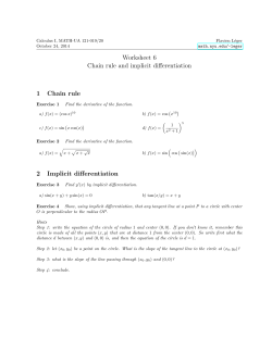
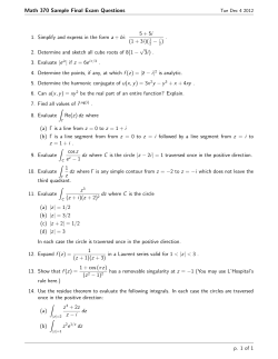
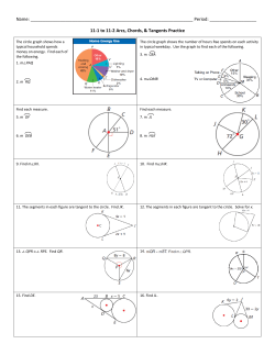
March 3, 2015
Time: 06:30pm
chapter1.tex
© Copyright, Princeton University Press. No part of this book may be
distributed, posted, or reproduced in any form by digital or mechanical
means without prior written permission of the publisher.
Chapter 1
Going in Circles
Question: How do you make a circle (and other curves)? The ancients knew how
to make a circle using a compass or its equivalent. I like to imagine an early genius tying
a piece of charcoal to one end of a string of plant fiber and drawing the charcoal along
a flat rock face while holding the other end of the string fixed. You can still do that,
but suppose that we want to enjoy modern technology and draw a circle on a computer
screen—a problem not faced in antiquity. How do we make a circle?
If you ask most people for the equation of a circle, you will probably hear
𝑥2 + 𝑦2 = 1 or perhaps (𝑥 − ℎ)2 + (𝑦 − 𝑘)2 = 𝑅2
for a circle with center (ℎ, 𝑘) and radius 𝑅. This is fine, but it represents a static view of
a circle, which is not the simplest way to direct the drawing of one.
The simplest way to instruct a machine to draw a circle uses a parametric form, also
known as a vector-valued function:
𝛾(𝑡) = (cos(𝑡), sin(𝑡))
for the unit circle and
𝛾(𝑡) = (ℎ + 𝑅 cos(𝑡), 𝑘 + 𝑅 sin(𝑡))
for a more general one. In either case, as the time parameter 𝑡 advances from 0 to 𝜋/2,
we climb the upper-left quadrant of the circle in a counterclockwise fashion. It takes 2𝜋
units of time to return to our starting point and complete the drawing.
The given formula parametrizes the circle in one particular way. If we need to be
more flexible, wanting to specify motion around a circle that starts at a particular point
and goes a particular direction, we can tweak the formula, perhaps by swapping the
coordinates or introducing minus signs, as in the following example.
Example: A Rolling Quarter
Place two quarters flat on the table with one above the other, both oriented right side
up. If the top one rolls without slipping around the other, find a formula for the motion
of the point that was originally at the bottom edge of the top circle.
Figure 1.1 shows the configuration before and after the quarter has rolled about 60∘ .
We use a letter 𝐹, as well as some dashed construction lines, to help you follow the
solution.
For general queries, contact [email protected]
March 3, 2015
Time: 06:30pm
chapter1.tex
© Copyright, Princeton University Press. No part of this book may be
distributed, posted, or reproduced in any form by digital or mechanical
means without prior written permission of the publisher.
SOLUTION. Suppose the quarter has radius 1 and has rolled so that the arc
length rolled out on each quarter is 𝑡. The position of the center of the rolling
quarter is then (2 sin(𝑡), 2 cos(𝑡)). This is what we meant by tweaking the formula:
When no arc length has been rolled out (𝑡 = 0), this vector should be pointing
straight up, and when 𝑡 is small and positive, the 𝑥-value should be increasing.
The formula matches.
Similarly, it takes a little work to figure out that the position of the rolling point
relative to the center of the rolling quarter is (− sin(2𝑡), − cos(2𝑡)). Here are a few
steps: In the diagram, the dashed lines might help you locate certain transversals.
These are key to showing that the angle up from the vertical is twice the angle 𝑡.
Adding the two vector displacements, we find that the desired vector motion is
𝛾(𝑡) = (2 sin(𝑡) − sin(2𝑡), 2 cos(𝑡) − cos(2𝑡)) ,
drawn on the top in Figure 1.2.
BEYOND THE ROLLING QUARTER. The path of the rolling quarter is an
example of a curve called an epicyloid, the curve produced by rolling one circle
around another. In general, if the fixed circle has radius 𝑎 and the rolling circle
has radius 1, the formula for the moving point is
Figure 1.1. Top: Initial position of rolling quarter.
Bottom: The quarter has rolled a bit and point X has
traced some of our curve, as if it dribbled a dot of red
ink on each point it passed over.
((𝑎 + 1) sin(𝑡) − sin((𝑎 + 1)𝑡), (𝑎 + 1) cos(𝑡) − cos((𝑎 + 1)𝑡)) .
(You may wish to show this as an exercise.)
Figure 1.2 shows two examples, the first with both circles the same size and the
second with one circle twice as large as the other.
Wheels on Wheels on Wheels
* EXERCISE 1
2𝜋
Apply the formula 𝐿 = ∫0 |𝛾󸀠 (𝑡)|𝑑𝑡 to
show that the arc length of the path of the
rolling quarter from our first example is 16
units.
Let’s think of the epicycloid as representing one particular kind of superposition
of circular motions, where we insist that the circles roll without slipping. If we
remove that restriction, we open the discussion to any sum of vector functions,
each of which represents a circular motion, possibly tweaked to turn a different
direction. I call this an instance of “wheels on wheels on wheels.”
To create a particular example, I chose some more or less random wheels
of different sizes and set them to turn at various rates, adding the vector
displacements to form the function
𝜇(𝑡) = (cos(𝑡) +
sin(6𝑡) cos(14𝑡)
cos(6𝑡) sin(14𝑡)
+
, sin(𝑡) +
+
).
2
3
2
3
The first term in each component is our familiar unit circle; the other terms
represent smaller wheels, one turning 6 times as fast, another 14 times as fast
and altered somehow (the sine and cosine functions are swapped). The result is
rendered in Figure 1.3. Take a moment to trace it with your eye and enjoy its
dancing undulations, realizing that probably none of us has the patience to draw
it without the aid of technology.
For general queries, contact [email protected]
2
Chapter 1
March 3, 2015
Time: 06:30pm
chapter1.tex
© Copyright, Princeton University Press. No part of this book may be
distributed, posted, or reproduced in any form by digital or mechanical
means without prior written permission of the publisher.
I hope that the figure—the “mystery curve”—surprises you. Nothing about the
numbers 6 and 14 prepares for the evident rotational symmetry, which means that
the figure is unchanged if we rotate it through 72∘ . Our next agenda item is to
answer the question: What causes this curve to have 5-fold rotational symmetry?
OUR COMPUTATIONAL PARADIGM. The formula for the mystery curve assigns one point of the Cartesian plane to every one of the infinitely many values of
the time parameter 𝑡. When I ask a computer to draw the curve, modern software
frees me from the need to figure out exactly how to instruct the computer to select
a mere finite few time values for which it places blobs of ink on the page or lighted
pixels on my screen. The details of computer graphics are lovely but are not the
purpose of this book; here, I invite us to be consumers, rather than inventors of
computer graphics.
In the instance of the mystery curve, a close examination of Figure 1.3 suggests
that I could have been a slightly more demanding consumer: At a few places on
the curve, I can detect that the machine has approximated the perfectly smooth
shape by some line segments. Since I know the curve bends smoothly, I don’t
object to this imperfection. I enjoy the availability of technology that can do
as well as it did. And if I wanted a finer rendition, I could have instructed the
machine to use more points in its drawing routing.
From the relatively simply mystery curve to the most complicated color image
in this book, the paradigm is the same: We look for mathematical objects, which
we will call smooth functions, that have some symmetry that we wish to illustrate,
perhaps the rotational symmetry of the mystery curve, perhaps something else.
Directing computers to make images of the discovered objects is not really
the interesting part of the process; it’s the finding of the class of symmetrical
things. This is what creating symmetry means to me: finding the formulas like
the one for the mystery curve—with its enigmatic 6 and 14—that will display
symmetrical images when rendered by software. It is not so much about the
method of computer rendition but the mathematical theory of what makes
things dance in the dazzling variety of patterned ways that we see in every
tradition of decorative art.
Figure 1.2. Two epicycloids: On the top is the locus
generated by the point on the rolling quarter; in the
bottom epicycloid, the rolling circle has half the
radius of the stationary one.
Some Ancient Mathematics
The trigonometric functions are not the only way to parametrize the circle. There
is some evidence that the ancient Babylonians knew a different way. It appears
that they knew how to find pairs of rational numbers 𝑥 and 𝑦 that solve the
equation 𝑥2 + 𝑦2 = 1, which, when we clear denominators, become what we
know as Pythagorean triples.
Much has been written about the history of a mysterious tablet called Plimpton
322, which lists, without any commentary that we can understand today, a
baffling array of Pythagorean triples [15]. Here we remark only that the vector
function
𝛾(𝑡) = (
2
1−𝑡
2𝑡
,
)
1 + 𝑡2 1 + 𝑡2
Figure 1.3. The mystery curve: What causes its
symmetry?
(1.1)
For general queries, contact [email protected]
Going in Circles
3
March 3, 2015
Time: 06:30pm
chapter1.tex
© Copyright, Princeton University Press. No part of this book may be
distributed, posted, or reproduced in any form by digital or mechanical
means without prior written permission of the publisher.
parametrizes the circle, as you can check with algebra, and that each coordinate is
a rational number if 𝑡 is rational. We could do the arithmetic by hand, but I found
it simpler to ask a machine to plug in 𝑡 = 54/125 to produce the Pythagorean
triple
12, 7092 + 13, 5002 = 18, 5412 .
This fact was apparently known to the Babylonians about 3800 years ago!
ANSWER FOR EXERCISE 1
2𝜋
Simplifying the square length of the velocity vector gives 𝐿 = ∫0 2√2 − 2 cos(𝑡)𝑑𝑡. Things look grim until we remember the trigonometric
2𝜋
identity that allows us to simplify the square root: 𝐿 ∫0 4 sin(𝑡/2)𝑑𝑡 = −4 ⋅ 2 cos(𝑡/2)|2𝜋
0 = 16 units.
For general queries, contact [email protected]
4
Chapter 1