
Earl et al - High Performance Computing
Resource
Assemblathon 1: A competitive assessment of de novo
short read assembly methods
Dent Earl,1,2 Keith Bradnam,3 John St. John,1,2 Aaron Darling,3 Dawei Lin,3,4
Joseph Fass,3,4 Hung On Ken Yu,3 Vince Buffalo,3,4 Daniel R. Zerbino,2 Mark Diekhans,1,2
Ngan Nguyen,1,2 Pramila Nuwantha Ariyaratne,5 Wing-Kin Sung,5,6 Zemin Ning,7
x Birol,10
Matthias Haimel,8 Jared T. Simpson,7 Nuno A. Fonseca,9 _Inanc
T. Roderick Docking,10 Isaac Y. Ho,11 Daniel S. Rokhsar,11,12 Rayan Chikhi,13,14
Dominique Lavenier,13,14,15 Guillaume Chapuis,13,14 Delphine Naquin,14,15
Nicolas Maillet,14,15 Michael C. Schatz,16 David R. Kelley,17 Adam M. Phillippy,17,18
Sergey Koren,17,18 Shiaw-Pyng Yang,19 Wei Wu,19 Wen-Chi Chou,20 Anuj Srivastava,20
Timothy I. Shaw,20 J. Graham Ruby,21,23 Peter Skewes-Cox,21,22,23 Miguel Betegon,21,23
Michelle T. Dimon,21,23 Victor Solovyev,24 Igor Seledtsov,25 Petr Kosarev,25
Denis Vorobyev,25 Ricardo Ramirez-Gonzalez,26 Richard Leggett,27 Dan MacLean,27
Fangfang Xia,28 Ruibang Luo,29 Zhenyu Li,29 Yinlong Xie,29 Binghang Liu,29
Sante Gnerre,30 Iain MacCallum,30 Dariusz Przybylski,30 Filipe J. Ribeiro,30 Shuangye Yin,30
Ted Sharpe,30 Giles Hall,30 Paul J. Kersey,8 Richard Durbin,7 Shaun D. Jackman,10
Jarrod A. Chapman,11 Xiaoqiu Huang,31 Joseph L. DeRisi,21,23 Mario Caccamo,26
Yingrui Li,29 David B. Jaffe,30 Richard E. Green,2 David Haussler,1,2,23
Ian Korf,3,32 and Benedict Paten1,2,33
1–32
[Author affiliations appear at the end of the paper.]
Low-cost short read sequencing technology has revolutionized genomics, though it is only just becoming practical for the
high-quality de novo assembly of a novel large genome. We describe the Assemblathon 1 competition, which aimed to
comprehensively assess the state of the art in de novo assembly methods when applied to current sequencing technologies.
In a collaborative effort, teams were asked to assemble a simulated Illumina HiSeq data set of an unknown, simulated
diploid genome. A total of 41 assemblies from 17 different groups were received. Novel haplotype aware assessments of
coverage, contiguity, structure, base calling, and copy number were made. We establish that within this benchmark: (1) It is
possible to assemble the genome to a high level of coverage and accuracy, and that (2) large differences exist between the
assemblies, suggesting room for further improvements in current methods. The simulated benchmark, including the
correct answer, the assemblies, and the code that was used to evaluate the assemblies is now public and freely available
from http://www.assemblathon.org/.
[Supplemental material is available for this article.]
Sequence assembly is the problem of merging and ordering shorter
fragments, termed ‘‘reads,’’ sampled from a set of larger sequences
in order to reconstruct the larger sequences. The output of an assembly is typically a set of ‘‘contigs,’’ which are contiguous sequence
fragments, ordered and oriented into ‘‘scaffold’’ sequences, with gaps
between contigs within scaffolds representing regions of uncertainty.
33
Corresponding author.
E-mail [email protected].
Article published online before print. Article, supplemental material, and publication date are at http://www.genome.org/cgi/doi/10.1101/gr.126599.111.
Freely available online through the Genome Research Open Access option.
2224
Genome Research
www.genome.org
There are numerous subclasses of assembly problems that can
be distinguished by, among other things, the nature of (1) the
reads, (2) the types of sequences being assembled, and (3) the
availability of homologous (related) and previously assembled sequences, such as a reference genome or the genome of a closely
related species (Pop and Salzberg 2008; Chaisson et al. 2009;
Trapnell and Salzberg 2009). In this work we focus on the evaluation of methods for de novo genome assembly using low-cost
‘‘short read’’ technology, where the reads are comparatively short
in length but large in number, the sequences being assembled
represent a novel diploid genome and the nearest homologous
genome to that being assembled is significantly diverged.
21:2224–2241 Ó 2011 by Cold Spring Harbor Laboratory Press; ISSN 1088-9051/11; www.genome.org
Assemblathon 1
In bioinformatics, the reads used in an assembly are derived
from an underlying sequencing technology. For a recent review of
sequencing technologies, see Metzker (2010). For the assembly
problem there are a number of key considerations, notably (1) the
length of the reads, (2) the error characteristics of the reads, (3)
whether and how the reads are ‘‘paired,’’ i.e., where reads are
produced in pairs separated by an approximately fixed length
spacer sequence, and finally (4) the number of reads produced for
a given cost.
Sanger sequencing (Sanger et al. 1977) produces relatively
long reads, typically between 300 and 1000 bp in length, with
a low error rate, but which are comparatively expensive to produce.
After relying primarily on Sanger sequencing for decades, the field
of sequencing has recently witnessed a diversification of competing technologies (Margulies et al. 2005; Bentley 2006; Pourmand
et al. 2006; Pandey et al. 2008; Eid et al. 2009) and a rapid rate of
overall change. One direction of this development has been
a move toward shorter reads, often #150 bp, but at a much lower
cost for a given volume of reads (Bentley 2006; Pourmand et al.
2006; Pandey et al. 2008).
As the field of sequencing has changed so has the field of
sequence assembly; for a recent review, see Miller et al. (2010). In
brief, using Sanger sequencing, contigs were initially built using
overlap or string graphs (Myers 2005) (or data structures closely
related to them) in tools such as phrap (http://www.phrap.org/),
GigAssembler (Kent and Haussler 2000), Celera (Myers et al. 2000;
Venter et al. 2001), ARACHNE (Batzoglou et al. 2002), and Phusion
(Mullikin and Ning 2003), which were used for numerous highquality assemblies such as human (Lander et al. 2001) and mouse
(Waterston et al. 2002). However, these programs were not generally efficient enough to handle the volume of sequences produced by the next-generation of sequencing technologies, spurring the development of a new generation of assembly software.
While some maintained the overlap graph approach, e.g.,
Edena (Hernandez et al. 2008) and Newbler (http://www.my454.
com/), others used word look-up tables to greedily extend reads,
e.g., SSAKE (Warren et al. 2007), SHARCGS (Dohm et al. 2007),
VCAKE ( Jeck et al. 2007), and OligoZip (http://linux1.softberry.com/berry.phtml?topic=OligoZip). These word look-up tables
were then extended into de Bruijn graphs to allow for global
analyses (Pevzner et al. 2001), e.g., Euler (Chaisson and Pevzner
2008), AllPaths (Butler et al. 2008), and Velvet (Zerbino and
Birney 2008). As projects grew in scale, further engineering was
required to fit large whole-genome data sets into memory (ABySS)
(Simpson et al. 2009), Chapman et al. (2011) (SOAPdenovo) (Li et al.
2010a), Cortex (in prep.). Now, as improvements in sequencer
technology are extending the length of ‘‘short reads,’’ the overlap
graph approach is being revisited, albeit with optimized programming techniques, e.g., SGA (Simpson and Durbin 2010), as are
greedy contig extension algorithms, e.g., PRICE (http://derisilab.
ucsf.edu/software/price/index.html), Monument (http://www.irisa.
fr/symbiose/people/rchikhi/monument.html).
In general, most sequence assembly programs are multistage
pipelines, dealing with correcting measurement errors within the
reads, constructing contigs, resolving repeats (i.e., disambiguating
false-positive alignments between reads), and scaffolding contigs
in separate phases. Since a number of solutions are available for
each task, several projects have been initiated to explore the parameter space of the assembly problem, in particular in the context
of short read sequencing (Phillippy et al. 2008; Alkan et al. 2011;
Hubisz et al. 2011; Lin et al. 2011; Narzisi and Mishra 2011; Zhang
et al. 2011). In this work we are concerned with evaluating as-
sembly programs as a whole, with the aim of comprehensively
evaluating different aspects of assemblies.
It is generally the case that the right answer to an assembly problem is unknown. Understandably therefore, a common
method for assessing assembly quality has been the calculation of
length summary statistics on the produced scaffold and contig
sequences. Such metrics include various weighted median statistics, such as the N50 defined below, as well as the total sequence
lengths and total numbers of sequences produced (Lindblad-Toh
et al. 2005; Ming et al. 2008; Church et al. 2009; Liu et al. 2009; Li
et al. 2010a; Colbourne et al. 2011; Locke et al. 2011).
Other methods have been proposed for evaluating the internal consistency of an assembly; for example, by analyzing the
consistency of paired reads, as in the clone-middle plot (Huson
et al. 2001), by looking for variations in the depths of read coverage
supporting a constructed assembly (Phillippy et al. 2008), and
looking at haplotype inconsistency (Lindblad-Toh et al. 2005).
To assess accuracy, assemblies may be compared with finished
sequences derived from independent sequencing experiments or
to sequences held out of the assembly process. For the dog genome,
nine bacterial artificial chromosomes (BACs) were sequenced to
finishing standards and held out of the assembly (Lindblad-Toh
et al. 2005), for the panda genome, which was primarily an Illumina assembly, extra Sanger sequencing of BACs was performed (Li
et al. 2010a). Additionally, if genetic mapping data is available,
such information can also be used to assess scaffold quality (e.g.,
Church et al. 2009), which used a combination of linkage, radiation hybrid, and optical maps. Church et al. (2009) also demonstrate that transcriptome (the set of RNA molecules for a given cell
type) information, if available, can also be used to assess the validity of a genomic assembly by checking the extent to which the
assembly recapitulates the transcriptome.
When a reference genome or sequence is available, a comparison between the assembly and reference can be performed.
This has previously been accomplished by studies using several
different genome alignment methods, including BLAST (e.g.,
Zhang et al. 2011), LASTZ (e.g., Hubisz et al. 2011), and Exonerate
(Hernandez et al. 2008; Zerbino and Birney 2008). Given such an
alignment, most simply, the proportion of a reference’s coverage
can be reported (Li et al. 2010b; Zhang et al. 2011). Notably, Gnerre
et al. (2011) compared novel short-read assemblies with the human and mouse reference genomes and performed a comprehensive set of analyses that encompassed coverage, contig accuracy,
and the long-range contiguity of scaffolds. Related to the work
described here, Butler et al. (2008) described a graph-based pattern
analysis using an assembly to reference alignment.
Comparison can also be made to a well-sequenced, related
species. This can be done using the complete genomic sequence of
an outgroup; for example, Meader et al. (2010) presented an assessment method based on patterns of insertions and deletions
(indels) in closely related interspecies genome alignments. Alternatively, specific genomic features can be studied; for example,
Parra et al. (2009) examined the fraction of ‘‘core genes,’’ those
present in all genomes, which could be identified in draft genome
assemblies.
Simulation has been a mainstay of genome assembly evaluation since assembly methodology was first developed and with
few exceptions (e.g., MacCallum et al. 2009; Gnerre et al. 2011) is
de rigueur when introducing new de novo assembly software (e.g.,
(Myers et al. 2000; Lander et al. 2001; Venter et al. 2001; Batzoglou
et al. 2002; Dohm et al. 2007; Jeck et al. 2007; Warren et al. 2007;
Butler et al. 2008; Chaisson and Pevzner 2008; Zerbino and Birney
Genome Research
www.genome.org
2225
Earl et al.
2008, etc.). In this work we have also chosen to use simulations,
utilizing the new Evolver genome evolution simulation tool
(http://www.drive5.com/evolver/) to produce a simulated diploid
genome with parameters that approximate that of a vertebrate
genome, though at ;1/10th of the scale.
From this novel genome we simulate reads, modeling an
Illumina sequencing run, using a newly developed read simulator.
Assembly teams were asked to assemble this novel genome blind,
and we present an analysis of the resulting assemblies. By using
simulation, we know a priori the haplotype relationships; by
a process of multiple sequence alignment (MSA) we assess the relationships between the assemblies and the original haplotypes of
our simulation. This novel process allows us evaluate haplotypespecific contributions to the assemblies. Additionally, as a positive
control for our results, we assess the generated assemblies using
more traditional BLAST (Hubisz et al. 2011; Zhang et al. 2011)
methods, and support our assessments by making all of the code
and data from our assessments public and freely available (http://
compbio.soe.ucsc.edu/assemblathon1/, http://www.assemblathon.
org/).
Results
We start by giving an overview of the Assemblathon 1 data set and
its generation. We then describe the assemblies before giving the
results of different evaluations.
Genome simulation
Rather than use an existing reference genome for assessment, we
opted to simulate a novel genome. We did this primarily for three
reasons. First, it gave us a genome that had no reasonable homology with anything other than out-group genomes that we
generated and provided to assemblers. This allowed for a fair, blind
test in which none of the assembly contributors had access to the
underlying genomes during the competition. Second, we were able
to precisely tailor the proportions of the simulated genome to
those desired for this experimental analysis, i.e., to limit the size of
the genome to less than that of a full mammalian genome, and
thus allow the maximum number of participants, while still
maintaining a size that posed a reasonable challenge. Third, we
could simulate a diploid genome; we know of no existing diploid
data set (simulated or real) in which the contributions of the two
haplotypes are precisely and fully known. This allowed us to assess
a heretofore-unexplored dimension of assembly assessment.
To simulate the genome we used the Evolver suite of genome
evolution tools. Evolver simulates the forward evolution of multichromosome haploid genomes and includes models for evolutionary constraint, protein codons, genes, and mobile elements.
The input genome for the simulation, termed the root genome,
was constructed by downloading the DNA sequence and annotations (see Methods) for human chromosome 13 (hg18/NCBI36,
95.6 non-N megabases [Mb]) from the UCSC Table Browser (Fujita
et al. 2011) and dividing it into four chromosomes of approximately equal length. Figure 1 shows the phylogeny used to generate the simulated genomes, with branch lengths to scale. We first
evolved the root genome for ;200 million years (my) to generate
the most recent common ancestor (MRCA) of the final leaf genomes. We performed this long burn-in on the genome in order to
reshuffle the sequence and annotations present, thereby preventing simple discovery of the source of the root genome. The simulation then proceeded along two independent lineages, generating
2226
Genome Research
www.genome.org
Figure 1. The phylogeny of the simulated haploid genomes. The root
genome derives from human chromosome 13. The a1 and a2 haplotypes
form the diploid genome from which we generated reads. The b1 and b2
haplotypes form a diploid out-group genome that was made available to
the assemblers.
both a and b, each ;50 my diverged from the MRCA. Finally, in
both lineages we split the evolved genome into two sublineages,
termed haplotypes, and evolved these sublineages for a further ;1
my, to produce a pair of diploid genomes, a1,2 and b1,2, each with
a degree of polymorphism. The a1,2 genome’s haplotypes, a1 and a2,
each had three chromosomes, and both haplotypes were 112.5 Mb
in total length with chromosome lengths of 76.3, 18.5, and 17.7 Mb.
The diploid a1,2 genome was used as the target genome for the
assembly. The b1,2 genome’s haplotypes, their common ancestor,
b, and their annotations, were provided to the assemblers as an
out-group. Relatively few assemblers (see Table 1) reported using
these sequences to assist in the assembly process.
Table 2A provides a count of some of the events that took
place along particular branches in the phylogenetic tree during the
course of the simulation. Table 2B provides a summary of the pairwise differences between the a1 and a2 haplotypes and Supplemental Figure 1 shows a dot-plot of their alignment. Supplemental
Figures 2 and 3 show the length distribution of annotations for the
root, MRCA, internal node, and leaf genomes, demonstrating that
these annotations remained approximately static over the course of
the simulation. We examined repeat content of the simulated genomes (see legend to Table 2) and found a comparable portion of
annotated repeats to that in the original human chromosome 13, but
a reduction of slightly more than half in the proportion of repetitive
100-mers (Supplemental Fig. 4). The simple substitution model used
by Evolver, which fails to capture some of the higher order dependencies in substitution patterns that made the original human
DNA sequence more repetitive, likely explains this latter observation.
Read simulation
As mentioned, there are many competing technologies now available for sequencing, giving us many possible options in designing
the data sets for the first Assemblathon. However, we opted to
simulate just one combined short read data set, with multiple read
libraries, for the Illumina Hi-seq platform (http://www.illumina.
com/systems/hiseq_2000.ilmn), which is the current market
leader for low-cost de novo sequencing on this scale. The advantage of this was chiefly (1) the avoidance of fragmentation in the
entries to the Assemblathon, thereby preventing categories with
few or just one entry, and (2) the ability to assess all of the submitted assemblies with common sets of evaluations.
We needed a program that would generate short reads and
model sources of error that the Illumina protocols introduce. As we
knew of no existing software that was capable of this (see Methods
for a discussion of existing read simulators), we wrote our own
short read simulator, called SimSeq (https://github.com/jstjohn/
SimSeq).
Abstractly, reads were sampled from the genome using one of
two types of Illumina-paired read strategy, so called ‘‘paired-end’’
Assemblathon 1
Table 1.
Groups that submitted assemblies
ID
ASTR
WTSI-P
EBI
WTSI-S
CRACS
BCCGSC
DOEJGI
IRISA
CSHL
DCISU
IoBUGA
UCSF
RHUL
GACWT
CIUoC
BGI
Broad
nVelv
nCLC
nABySS
Affiliations
Entries
Software
Used b
Agency for Science, Technology, and Research, Singapore
Wellcome Trust Sanger Institute, UK
European Bioinformatics Institute, UK
Wellcome Trust Sanger Institute, UK
Center for Research in Advanced Computing Systems, Portugal
BC Cancer Genome Sciences Center, Canada
DOE Joint Genome Insititute, USA
L’IRISA (Institut de recherche en informatique et syste`mes
ale´atoires), France
CSHL (Cold Spring Harbor Laboratory), USA
Department of Computer Science, Iowa State University
Computational Systems Biology Laboratory, University
of Georgia, USA
UC San Francicso, USA
Royal Holloway, University of London, UK
The Genome Analysis Center, Sainsbury Laboratory,
and Wellcome Trust Center for Human Genetics, UK
Department of Computer Science, University of Chicago, USA
BGI, Shenzhen China
Broad Institute
—
—
—
1
2
2
4
3
5
1
5
PE-Assembler
Phusion2, phrap
SGA, BWA, Curtain, Velvet
SGA
ABySS
ABySS, Anchor
Meraculous
Monument
No
No
No
No
Yes
No
No
No
2
1
3
Quake, Celera, Bambus2
PCAP
Seqclean, SOAPdenovo
Noa
No
No
1
5
3
PRICE
OligoZip
Cortex_con_rp
Yes
No
No
1
1
1
6
9
6
Kiki
SOAPdenovo
ALLPATHS-LG
Velvet
CLC
ABySS
No
No
No
No
No
No
The first 17 rows in the table correspond to entries submitted by participants in the competition. Assemblies with IDs beginning with ‘‘n,’’ (for naive),
were generated by organizers of the competition to demonstrate the performance of popular programs run with variations on their default parameters.
a
CSHL.1 used the b genome though that team’s top assembly, CSHL.2, which is referred to in the main paper as CSHL, did not.
though the specific choice of E. coli and the 5% level were arbitrary.
Participants in the contest were notified that some bacterial contamination was present in the data, though they were not told
about its precise nature nor explicitly told to remove it.
Multiple libraries were generated for both the paired-end and
mate-pair strategies. Paired-end libraries with 200- and 300-bp
inserts contributed 803, mate-pair libraries with separations of 3
and ‘‘mate-pair’’ strategies, after which an error profile was applied
to each read in its proper orientation. In addition to generating
reads from the target a1,2 genome, three copies of an Escherichia coli
sequence (gi 312944605) were added to the two haplotype sequences to yield a ;5% bacterial contamination rate. Bacterial
sequence was included as an attempt to model the sort of contamination occasionally present in data from sequencing centers,
Table 2.
Genome simulation statistics
(A)
Genome
Input
MRCA
a
a1
a2
b
b1
b2
Reps
100mer (%) Chr
Mb
GC (%)
Reps (%)
95.6
109.4
112.4
112.5
112.5
112.3
112.4
112.4
38.8
39.9
40.0
40.0
40.0
40.0
40.0
40.0
7.1 / 42.3a
6.9
7.5
7.5
7.5
6.8
6.8
6.8
0.8
0.3
0.3
0.3
0.3
0.3
0.3
0.3
4
2
3
3
3
2
2
2
Subs
–
35.9 3
9.70 3
1.97 3
1.97 3
9.71 3
1.97 3
1.97 3
Dels
Inv
–
–
106 2.47 3 106 11,701
106 6.72 3 105
3325
105
13,528
54
5
10
13,834
61
6
5
3313
10 6.74 3 10
5
10
13,632
64
105
13,621
71
Moves
–
4714
1369
34
31
1325
26
35
Copy
Tandem
–
–
14,644 1.16 3 106
4151 3.13 3 105
83
6436
80
6494
4043 3.14 3 105
82
6354
79
6445
Chr split Chr fuse
–
2
1
0
0
0
0
0
4
0
0
0
0
0
0
(B)
Comparison
a1 a2
SNPs
Subs
+ Subs
Indels
+ Indels
Inv
439,385
441,796
444,247
29,972
521,142
115
(A) Event numbers are between the previous branch point and the named node. (Mb) Size of the genome in megabases; (GC) percentage GC content;
(Reps) percent of the genome masked by the union of tandem repeats finder and RepeatMasker; (Reps 100-mer) percent repetiteveness of the sequence
and its reverse complement for 100-mers calculated with the tallymer tool (Kurtz et al. 2008); (Chr) number of chromosomes; (Subs) number of substitution events; (Dels) number of deletion events; (Inv) number of inversion events; (Moves) number of translocations; (Copy) number of DNA segmental
duplications; (Tandem) number of tandem repeat insertions; (Chr split) number of chromosome fission events; (Chr fuse) number of chromosome fusion
events.
a
The published value for chromosome 13 (Dunham et al. 2004).
(B) Differences between haplotypes a1 and a2 as determined by inspection of the Evolver pairwise alignment. (SNPs) Count of single nucleotide polymorphisms; (Subs) count of substitutions, including SNPs; (S Subs) sum of the lengths of all substitutions; (Indels) count of insertion deletion events; (S
Indels) sum of the lengths of all insertion deletion events; (Inv) the sum of number of inversions invoked in each of the a1 and a2 Evolver steps.
Genome Research
www.genome.org
2227
Earl et al.
and 10 kb contributed a further 403, giving a total coverage of
1203 for the sample. Removing contamination reads gave an
overall coverage of ;553 per haplotype.
A detailed description of the simulation method, the types of
errors simulated, and the simulator’s limitations are given in the
Methods section. Importantly, due to human error, the error model
was mistakenly reversed along the reads. This resulted in bases
with a slightly higher error rate tending to appear toward the beginning of the reads rather than toward the end of reads (see
Supplemental Fig. 5). This issue only manifests itself if the reads are
treated asymmetrically; we surveyed participants on this matter
and only one group, L’IRISA, indicated that their methodology was
possibly harmed more than other methods due to the mistake.
Assemblies
The competition started in January 2011 and teams were given just
over 1 mo to submit their assemblies. Teams were allowed to submit up to five separate assemblies for consideration. Additionally,
assemblies were created by the organizers with popular assembly
programs, using default parameters, as a way of comparing naively
generated assemblies with those that were contributed by independent groups. Table 1 lists the evaluated assemblies, the main
program used to generate them, and the groups that contributed
them (see Supplemental section 8.2 for detailed information on
submissions). In total there were 59 assemblies, with 41 independently contributed by 17 different groups using 15 different
assembly programs and 18 generated by the organizers using three
popular programs.
Evaluations
We assessed all of the contributed assemblies, full results for which
can be found in the Supplemental material. However, to make the
presentation succinct we choose to present only the ‘‘top’’ as-
sembly from each group in the following evaluations. To enable
this we created a ranking of the assemblies (see Table 3; Supplemental Table 1), using the evaluations described below, and selected the assembly from each group with the top overall ranking
for inclusion. Full results for each evaluation on every assembly in
the main text can be found in the Supplemental material.
N50 and NG50
A commonly used metric to assess assemblies is the N50 statistic.
The N50 of an assembly is a weighted median of the lengths of the
sequences it contains, equal to the length of the longest sequence
s, such that the sum of the lengths of sequences greater than or
equal in length to s is greater than or equal to half the length of the
genome being assembled. As the length of the genome being assembled is generally unknown, the normal approximation is to use
the total length of all of the sequences in an assembly as a proxy for
the denominator. We follow this convention for calculating N50,
but additionally we define the NG50 (G for genome). The NG50 is
identical to N50, except that we estimate the length of the genome
being assembled as being equal to the average of the length of the
two haplotypes, a1 and a2. Contig N50s and NG50s, where the
sequences are the set of assembly contigs, and scaffold N50s and
NG50s, where the sequences are the set of assembly scaffolds, are
shown in Figure 2, Supplemental Figure 6, and Supplemental Table 2.
The total span of most of the submitted assemblies was
slightly larger than the haploid genome size, primarily because of
the degree of polymorphism of the two haplotypes. Thus, the assembly-specific N50s are in general smaller than the NG50s, with
the median absolute difference between contig NG50 and contig
N50 being 599 bp (7.7%), and the median absolute difference between scaffold NG50 and scaffold N50 being 1942 bp (3.6%).
These differences are quite small, though not negligible in every
case; for example, the CSHL assembly has a scaffold NG50 ;800 kb
(31.6%) longer than scaffold N50.
Table 3.
Rankings of the top assembly from each team in eight categories
ID
Overall
Broad
BGI
WTSI-S
DOEJGI
CSHL
CRACS
BCCGSC
EBI
IoBUGA
RHUL
WTSI-P
DCSISU
nABySS
IRISA
ASTR
nVelv
nCLC
UCSF
GACWT
CIUoC
31
37
38
44
57
58
60
64
65
71
74
99
100
103
106
114
115
138
149
152
CPNG50
2
1
9
14
3
11
5
16
7
6
4
12
10
17
8
18
15
12
20
19
(7.25
(8.23
(2.48
(1.15
(4.23
(1.55
(3.63
(9.39
(3.06
(3.20
(3.80
(1.35
(1.99
(8.20
(2.52
(5.65
(9.47
(1.35
(2.53
(5.60
3
3
3
3
3
3
3
3
3
3
3
3
3
3
3
3
3
3
3
3
104)
104)
104)
104)
104)
104)
104)
103)
104)
104)
104)
104)
104)
103)
104)
103)
103)
104)
103)
103)
SPNG50
3
6
1
2
8
5
4
7
12
13
11
10
16
9
14
15
18
17
19
20
(2.11
(1.17
(4.95
(4.86
(7.17
(1.44
(1.46
(1.13
(3.54
(3.31
(4.21
(5.61
(2.00
(5.82
(3.13
(2.75
(9.54
(1.35
(7.82
(5.60
3 105)
3 105)
3 105)
3 105)
3 104)
3 105)
3 105)
3 105)
3 104)
3 104)
3 104)
3 104)
3 104)
3 104)
3 104)
3 104)
3 103)
3 104)
3 103)
3 103)
Struct
3 (1244)
6 (1878)
2 (475)
1 (456)
14 (5146)
4 (1666)
10 (2867)
7 (2055)
15 (6310)
8 (2551)
13 (4895)
12 (4319)
5 (1731)
11 (3725)
9 (2818)
18 (8626)
16 (7283)
20 (24,987)
17 (8622)
19 (11,282)
CC50
1 (2.66
7 (5.66
3 (1.14
2 (1.89
6 (6.11
4 (8.61
8 (3.22
9 (3.04
5 (6.47
15 (1.59
13 (3.41
12 (9.75
16 (6.97
9 (3.04
14 (1.81
11 (1.27
18 (4.36
17 (6.84
19 (2.60
20 (1.27
3 106)
3 105)
3 106)
3 106)
3 105)
3 105)
3 105)
3 105)
3 105)
3 104)
3 104)
3 104)
3 103)
3 105)
3 104)
3 105)
3 103)
3 103)
3 103)
3 103)
Subs
4
11
1
3
9
2
8
6
15
5
14
13
7
17
12
18
10
20
16
19
(2.92
(1.20
(1.30
(4.43
(1.02
(3.81
(7.00
(5.17
(3.80
(3.52
(1.48
(1.37
(5.96
(3.99
(1.28
(6.21
(1.11
(1.21
(3.86
(1.11
3
3
3
3
3
3
3
3
3
3
3
3
3
3
3
3
3
3
3
3
Copy num
10
10
10
10
10
10
10
10
10
10
10
10
10
10
10
10
10
10
10
10
6
)
)
7
)
7
)
5
)
7
)
6
)
6
)
5
)
6
)
5
)
5
)
6
)
5
)
5
)
5
)
5
)
4
)
5
)
4
)
5
11
2
9
7
6
12
15
1
3
5
4
13
19
14
18
10
8
17
20
16
(6.71
(6.75
(5.74
(5.42
(4.95
(6.82
(1.17
(3.56
(8.38
(4.77
(4.38
(6.91
(3.17
(7.61
(2.88
(6.22
(5.61
(2.30
(3.46
(1.98
3
3
3
3
3
3
3
3
3
3
3
3
3
3
3
3
3
3
3
3
10
10
10
10
10
10
10
10
10
10
10
10
10
10
10
10
10
10
10
10
Cov tot
2
)
)
)
2
)
2
)
2
)
1
)
3
)
3
)
2
)
2
)
2
)
1
)
2
)
1
)
2
)
2
)
1
)
1
)
1
)
3
2
6
1
8
11
4
14
2
9
6
4
2
15
10
16
17
13
12
19
18
20
(98.3)
(98.8)
(97.8)
(97.3)
(98.5)
(96.3)
(98.7)
(97.7)
(98.3)
(98.5)
(98.7)
(94.3)
(97.5)
(93.7)
(90.9)
(96.5)
(97.2)
(83.7)
(86.4)
(78.5)
Cov genic
1 (93.8)
3 (92.7)
5 (91.8)
4 (92.3)
7 (89.1)
6 (90.2)
8 (88.9)
9 (88.5)
2 (92.8)
15 (67.4)
13 (75.0)
12 (79.0)
17 (57.2)
10 (88.1)
14 (68.5)
11 (84.8)
18 (55.4)
16 (59.6)
20 (48.0)
19 (48.9)
For each category (listed below), all of the received assemblies were ranked. The sum of the rankings from each category was then used to create an
overall rank for the assemblies, the top-ranked (lowest number) assembly from each group was then selected for inclusion in this manuscript. Numbers
are ranks, with values shown in parentheses. (Overall) Sum of all rankings (possible range 8–160); (CPNG50) contig path NG50; (SPNG50) scaffold path
NG50; (Struct) sum of structural errors; (CC50) length for which half of any two valid columns in the assembly are correct in order and orientation; (Subs)
total substitution errors per correct bit; (Copy num) proportion of columns with a copy number error; (Cov tot) overall coverage; (Cov genic) coverage
within coding sequences.
2228
Genome Research
www.genome.org
Assemblathon 1
section 7.1, and references to which are
made below.
Coverage
An MSA can be divided up into columns,
each of which represents a set of individual base-pair positions in the input
sequences that are considered homologous. We call columns that contain positions within the haplotypes haplotype
columns. We define the overall coverage of
an MSA as the proportion of haplotype
columns that contain positions from the
assembly. Similarly, we can define the
coverage of X, where X is a specific haplotype or the bacterial contamination, as
the proportion of columns containing
positions in X that also contain positions
from the assembly.
Table 4 shows the overall, haplotype-specific, and bacterial contamination-specific coverage. There is very little
difference between the specific haplotype’s coverage and the overall coverage
and, indeed, little difference between
many of the assemblies. The highest
Figure 2. N50 statistics. Assemblies are sorted left to right in descending order by scaffold path NG50.
overall coverage was the BGI assembly
Data points for each assembly are slightly offset along the x-axis in order to show overlaps.
with 98.8%, but nearly all assemblies
performed well in this metric with even
Multiple sequence alignment
the assembly with 14th highest coverage, the CRACS assembly,
providing 96.3% coverage. However, there were huge differences
While N50 statistics give a sense of the scale and potential contiin the coverage of the bacterial contamination (Supplemental
guity of an assembly, they say nothing necessarily about the unFigs. 7, 8), with many groups opting successfully to completely
derlying coverage or accuracy of an assembly. To compare each
filter it out. For example, the BGI assembly had no coverage of the
assembly with the simulated genome and bacterial contamination
bacterial sequence, while the ASTR assembly had 100.0% coverwe constructed a multiple sequence alignment (MSA). The seage of the bacterial sequence.
quence inputs to the MSA were the two
haplotypes, the bacterial contamination,
and the scaffolds of the assembly. To Table 4. Coverage statistics for the top assembly from each team
generate the MSA we used an adapted
Hap a2 (%)
Bac (%)
Genic (%)
Unmapped
ID
Hap total (%)
Hap a1 (%)
version (see Methods) of the newly developed Cactus alignment program (Paten
BGI
98.8
98.9
98.8
0.0
92.7
2.637 3 105
et al. 2011b), a new MSA program able BCCGSC
98.7
98.7
98.7
99.9
88.9
6.546 3 106
to handle rearrangements, copy-number WTSI-P
98.7
98.7
98.7
99.8
75.0
5.369 3 106
98.5
98.5
98.5
100.0
67.4
4.961 3 106
changes (duplications), and missing data. RHUL
CSHL
98.5
98.6
98.5
99.9
89.1
7.815 3 106
The result of this alignment process was,
Broad
98.3
98.4
98.3
68.9
93.8
3.538 3 106
for each assembly, a high-specificity IoBUGA
98.3
98.3
98.3
4.8
92.8
7.822 3 105
map of the alignment of the assembly WTSI-S
97.8
97.8
97.8
99.1
91.8
4.948 3 106
97.7
97.7
97.7
0.9
88.5
4.553 3 105
to the two haplotypes and the bacterial EBI
nABySS
97.5
97.5
97.5
99.8
57.2
1.111 3 107
contamination.
DOEJGI
97.3
97.4
97.3
99.5
92.3
5.304 3 106
As we aligned both the bacterial nCLC
97.2
97.2
97.2
99.8
55.4
5.673 3 106
contamination and the two haplotypes
nVelv
96.5
96.6
96.5
99.8
84.8
8.028 3 106
96.3
96.3
96.3
99.8
90.2
5.265 3 106
together, we used the hypothetical exis- CRACS
94.3
94.3
94.2
99.5
79.0
6.259 3 106
tence of any alignments between the DCSISU
IRISA
93.7
93.7
93.7
99.7
88.1
5.426 3 106
haplotypes and the bacterial contamina- ASTR
90.9
90.9
90.9
100.0
68.5
5.175 3 106
tion as a negative control for nonspe- GACWT
86.4
86.4
86.4
0.0
48.0
2.053 3 106
83.7
83.7
83.7
0.0
59.6
1.822 3 106
cific alignment. We did not observe UCSF
CIUoC
78.5
79.0
78.1
0.6
48.9
3.638 3 105
any such alignments. As an additional
control we replicated a similar, confir(Hap total) Overall coverage; (Hap a1) percent coverage for Haplotype a1; (Hap a2) percent coverage
matory analysis using a simple BLAST for Haplotype a ; (Bac) percent coverage
of the bacterial contamination; (Genic) percent coverage of
2
(Altschul et al. 1990) strategy, details of the coding sequences; (Unmapped) number of unmapped bases, many corresponding to short
which can be found in Supplemental contigs.
Genome Research
www.genome.org
2229
Earl et al.
Blocks and contig paths
Within an MSA a block is a maximal gapless alignment of a set of
sequences and is therefore composed of a series of contiguous
columns. The length of a block is equal to the number of columns
that it contains. We can use the block structure to define the block
NG50, which is exactly like the NG50, except that we use the
distribution of block lengths rather than sequence lengths. Supplemental Figures 9 and 10 show block coverage across the haplotypes. Alignment of sequences that are very closely related are
likely to contain fewer blocks with a greater base-pair length than
sequences that are significantly diverged from one another. Unfortunately, the two simulated haplotypes are sufficiently polymorphic with respect to one another, which the block NG50 of an
alignment of just the two haplotypes is ;4 kb. As this length is
much less than the length of many sequences in the assemblies,
assessing an assembly requires methods that do not penalize the
reconstruction of haplotype-specific polymorphisms. This is evident by looking at Figure 2, which shows that block NG50 is poorly
discriminative. See Supplemental section 7.1.1 and Supplemental
Figure 11 for supporting BLAST based analysis.
To extend our analysis we use a graph theoretic model of the
alignments, which we now describe in overview. An MSA can be
described as a graph, and we call the simplest such graph an adjacency graph. A formal description of the adjacency graph used
here can be found in Paten et al. (2011a), it is closely related to the
similarly named graph introduced in Bergeron et al. (2006a), but
also to a directed bigraph representation of a de Bruijn graph used
in assembly (Medvedev and Brudno 2009) and the multiple
breakpoint graph used in the study of genome rearrangements
(Alekseyev and Pevzner 2009).
An adjacency graph G contains two kinds of edges, block edges,
which represent the gapless blocks of the alignment, and adjacency
edges, which represent collections of connections between the
ends of segments of DNA. The nodes in the graph represent the
ends of blocks of aligned sequences. Figure 3 illustrates an example.
Each edge in G is labeled with the subsequences it represents,
called segments; thus, it is possible to discern whether the edge
represents segments in the haplotypes, the assembly, the bacterial
contamination or some combination. As previously stated, no
edges are contained in G that represent segments in both the
haplotypes and the bacterial contamination.
Within G, a sequence is represented as a path of alternating
adjacency and block edges, termed a thread. We can assess the accuracy of assembly sequences by analyzing their thread representation in the adjacency graph. Let P be the thread representing an
assembled sequence in G. Any edge e in P is consistent if that edge is
also labeled with segments from either or both of the haplotypes.
For any P, a contig path is a maximal subpath of P in which all the
edges are consistent. Thus, P can be divided up into a series of
contig paths, possibly interspersed with edges in P that are not
contained in a contig path, see Figure 3 for an example. The basepair length of a contig path is equal to the sum of the base-pair
lengths of the block edges it contains. Contig paths represent
maximal portions of the assembled sequence that are consistent
with one or both of the haplotypes and contain no assembly
gaps, they can be thought of as portions of an assemblies’ contigs
that perfectly follow a path through the graph of haplotype
polymorphism.
Figure 2 shows contig path NG50s, defined analogously to
block NG50; Supplemental Figures 12 and 13 show contig path
coverage across the haplotypes, while Supplemental Figures 14 and
15 show, in contrast, the same plots, but instead use raw contig
lengths. The contig path NG50s are substantially larger than block
NG50s; for example, the BGI assembly has a contig path NG50 1.5
orders of magnitude bigger than its block NG50. The difference
between the largest and smallest block NG50 is 2556 bp (GACWT
1351 bp to BGI 3907 bp); the difference between the largest and
smallest contig path NG50 is 79,731 bp (GACWT 2533 bp to BGI
82,264 bp). Thus, the contig path NG50 results demonstrate that
assemblies are able to reconstruct substantial regions perfectly,
and contig path NG50 appears to be a more discriminative statistic than block NG50, as it indicates large differences between the
assemblies.
Scaffold paths
To account for gaps within scaffolds, which we henceforth call
scaffold breaks, we define scaffold paths. Scaffold paths can be
thought of as portions of the assemblies’ scaffolds that perfectly
follow a path through the graph of haplotype polymorphism, but
which are allowed to jump unassembled sequences at scaffold gaps.
Scaffold gaps are scaffold breaks (denoted as contiguous runs of
wild-card characters in an assembly) whose surrounding contig
ends are bridged by a path of haplotypes representing edges within
the adjacency graph; see Figure 3 for an
example and the Methods section for
a formal definition.
Notably, our definition of a scaffold
gap within the graph is permissive in that
it allows (1) any sequence of Ns to define
a scaffold break, and (2) the sequence of
Ns that define the scaffold break to be
Figure 3. An adjacency graph example demonstrating threads, contig paths, and scaffold paths.
aligned within the ends of the block that
Each stack of boxes represents a block edge. The nodes of the graph are represented by the left and right
sandwich the gap in the assembly. This
ends of the stacked boxes. The adjacency edges are groups of lines that connect the ends of the stacked
definition was sought because there is
boxes. Threads are represented (inset) within the graph as alternating connected boxes and colored
lines. There are three threads shown: (top to bottom) black, gray, and light gray. The black and gray
currently a wide variation in the syntax
threads represent two haplotypes; there are many alternative haplotype threads that result from
used to define such gaps within different
a mixture of these haplotype segments, which are equally plausible given no additional information to
assemblers, and to be tolerant of aligndeconvolve them. The light-gray thread represents an assembly sequence. For the assembly thread,
ment errors caused by the phenomena of
consistent adjacencies are shown in solid light gray. The dashed light gray line between the right end of
block g and the left end of block i represents a structural error (deletion). The dashed light-gray line
edge wander (Holmes and Durbin 1998)
between the right end of block k and the left end of block m represents a scaffold gap, because the
caused when the alignment of positions
segment of the assembly in block n contains wild-card characters. The example, therefore, contains
around a gap has more than one equally
three contig paths: (from left to right) blocks a. . .g ACTGAAATCGGGACCCC; blocks i, j, k GGAAC; and
probable scenario. As a scaffold path is
block m CC. However, the example contains only two scaffold paths because the latter two contig paths
are concatenated to form one scaffold path.
a concatenation of contig paths, its base-
2230
Genome Research
www.genome.org
Assemblathon 1
pair length is just the sum of the base-pair lengths of the contig
paths that it contains.
Figure 2 shows the scaffold path NG50, defined analogously
to the block and contig path NG50s, sorted with respect the scaffold NG50. In many cases the scaffold path NG50 is substantially
larger than the contig path NG50. Figure 4 shows a stack fill plot of
the coverage of scaffold paths along the three chromosomes of
haplotype a1 (see also Supplemental Figs. 16–19). It demonstrates
the substantial differences between the assemblies and shows that
large, megabase regions of the haplotype can be reconstructed with
assembly gaps, but without apparent error.
Structural errors
Despite the long lengths of many scaffold paths, for most assemblies the scaffold NG50 is substantially larger than the scaffold
path NG50, indicating that there were apparent errors that broke
scaffolds into smaller sets of scaffold paths. To analyze these errors
we continued our graph analysis, defining a number of subgraph
types to represent them, which we formally define in the Methods
section. These subgraph definitions include erroneous intra- and
interchromosomal joins, insertions, deletions, simultaneous insertion and deletions, and insertions at the ends of assembled se-
quences. Table 5 (and Supplemental Table 3) shows the numbers of
structural errors for each assembly; Supplemental Figures 20 and
21 show structural errors across the haplotypes. Many assemblies
do not have categories of error to which they are particularly
prone, but a few do. In these cases there may be a systematic bias in
the operation of the programs that generated them or in the way
that we interpreted them.
Insertion and deletion (indel) structural errors involve, respectively, the addition and removal of a contiguous run of bases.
In Supplemental Figures 22 and 23 we investigate the size distribution of such errors, using both the described MSA and supporting alignments from the progressiveMauve program (Darling
et al. 2010). We find that in almost all cases, the size distribution of
the segments of inserted and deleted bases follows an approximately geometrically decreasing distribution.
We also searched for subgraphs in which the assembly created
a haplotype to contamination chimera, but did not find any such
subgraphs. To investigate this surprising result we searched for
such chimeras using BLAST with relaxed parameters (Supplemental section 7.1.3; Supplemental Fig. 24). Using this approach we
found 56 assemblies with no such chimeras, seven assemblies with
1 chimera, one assembly with two chimeras, and one outlier assembly with 26 chimeras. In each case we verified that these chi-
Figure 4. Assembly coverage along haplotype a1 stratified by scaffold path length weighted overall coverage. The top six rows show density plots of
annotations. (CDS) Coding sequence; (UTR) untranslated region; (NXE) nonexonic conserved regions within genes; (NGE) nongenic conserved regions;
(island) CpG islands; (repeats) repetitive elements. The remaining rows show the top-ranked assembly from each group, sorted by scaffold path length
weighted overall coverage. Each such row is a density plot of the coverage, with colored stack fills used to show the length of scaffold paths mapped to
a given location in the haplotype. For example, the left-most light-orange block of the WTSI-S assembly row represents a region of haplotype a1 that is
almost completely covered by a scaffold path from the WTSI-S assembly greater than one megabase in length.
Genome Research
www.genome.org
2231
Earl et al.
Table 5.
ID
Structural error statistics for the top assembly from each team
Intrachromosomal
joins
Interchromosomal
joins
Insertions
Deletions
Insertion and
deletion
Insertion at
ends
+ errors
21
6
75
687
17
368
458
691
2065
351
147
1410
1940
396
919
23
757
2885
1205
2731
160
191
161
303
48
288
563
349
200
285
203
956
449
337
330
64
730
455
684
2396
55
56
524
198
208
355
127
172
109
255
925
330
1851
417
1663
2359
905
1473
1,189
5908
108
76
379
121
188
639
547
264
227
233
1593
954
289
3287
2933
2237
1292
2838
2026
6223
40
19
9
51
63
98
53
26
73
102
116
109
87
223
356
68
216
306
65
1018
72
127
96
306
1207
130
307
1049
144
1641
741
560
279
486
109
2532
4722
669
6113
6711
456
475
1244
1666
1731
1878
2055
2551
2818
2867
3725
4319
4895
5146
6310
7283
8622
8626
11,282
24,987
DOEJGI
WTSI-S
Broad
CRACS
nABySS
BGI
EBI
RHUL
ASTR
BCCGSC
IRISA
DCSISU
WTSI-P
CSHL
IoBUGA
nCLC
GACWT
nVelv
CIUoC
UCSF
Columns are defined in the main text.
meras were missed in the graph approach due to the stringent MSA
parameters.
Long-range contiguity
Annotation analysis
Evolver maintains annotations for a number of classes of simulated
sequence, including genes, which Evolver models as having exons,
introns, and untranslated regions (UTRs), and conserved noncoding
elements. Additionally, while Evolver does not track the history of
individual repeat elements following their insertion, it maintains
The MSA graph theoretic analysis we have described is local in
nature and quite strict, in that it has no notion of large-scale
contiguity and refuses to stitch together
paths that would be joined, but for a
small error. We thus sought a method to
analyze the larger scale contiguity between pairs of separated points in the
genome. Formally, for two positions xi
and xj in a haplotype chromosome x,
such that i < j, if there exists two positions
yk, yl in an assembly scaffold y such that
(1) yk is in the same column as xi, (2) yl is
in the same column as xj, and (3) k < l, we
say yk and yl are correctly contiguous. Pairs
may be correctly contiguous but not
necessarily covered by the same contig
path or scaffold path, and indeed there
may be arbitrary numbers of assembly
errors between two correctly contiguous
positions.
Figure 5 shows the proportion of
correctly contiguous pairs as a function of
the pairs’ separation distance for each
assembly. Taken at a high level, in all of
the assemblies the proportion of correctly
linked pairs monotonically decreases with
separation distance. Therefore, we take
the separation distance at the 50th percentile, termed the correct contiguity 50
(CC50) as an essentially sufficient statis- Figure 5. The proportion of correctly contiguous pairs as a function of their separation distance. Each
line represents the top assembly from each team. Correctly contiguous 50 (CC50) values are the lowest
tic. See Supplemental section 7.1.2 and point of each line. The legend is ordered top to bottom in descending order of CC50. Proportions were
Supplemental Figures 25 and 26 for sup- calculated by taking 100,000,000 random samples and binning them into 2000 bins, equally spaced
along a log10 scale, so that an approximately equal number of samples fell in each bin.
porting BLAST-based analysis.
2232
Genome Research
www.genome.org
Assemblathon 1
a library of mobile elements, and thus, using RepeatMasker (v1.25
http://www.repeatmasker.org) and tandem repeats finder (v4.0,
http://tandem.bu.edu/trf/trf.html) with this library, we identified
a subset of repetitive sequence within the haplotypes.
Continuing the previous MSA analysis, we define a perfect
path as a maximal subpath of a haplotype thread that is isomorphic
to a subpath of an assembly thread. For a given assembly, the
corresponding set of perfect paths reflects the regions of the haplotypes that are perfectly reconstructed. Unlike contig and scaffold
paths, perfect paths are intolerant of haplotype polymorphism,
but give a well-defined set of intervals within a1,2 for comparison
with a set of annotations. Table 6 shows for each assembly the
proportion of each annotation type contained within perfect
paths.
Both haplotypes of the a1,2 genome contain 176 proteincoding genes, Supplemental Figure 27 show the distribution of
their lengths; we find that only a small proportion (max 11% of
base pairs, min 2% of base pairs) of these full-length transcripts are
perfectly reconstructed by the assemblies. Conversely, we find that
in the best assemblies almost all exons and a high proportion of
UTRs are perfectly reconstructed, for example, 99% of base pairs in
exons and 84% of base pairs in UTRs of the BGI assembly. We also
find that most perfectly reconstructed genes are intronless (data
not shown); the assemblies therefore fail mostly to reconstruct
introns perfectly. To further characterize this failure we used
tBLASTN (Altschul et al. 1990; see Supplemental section 7.1.4) to
align the spliced transcripts of a1 (without introns and UTRs) to the
scaffolds of the assemblies, counting a match if it included 95% of
the given transcript; see last column of Table 4, labeled genic correctness, and Supplemental Table 1. This more tolerant analysis
reveals that in the best assemblies the majority of exon chains are
reconstructed contiguously (in the correct order and orientation)
within single scaffolds, e.g., the Broad assembly has 107 spliced
transcripts (93.8% of base pairs) reconstructed by this metric.
As expected, repeats were the least well-reconstructed annotation types, with the best assembly, BGI, reconstructing only 64%
of repeats perfectly (see last column of Table 6). As these regions are
naturally difficult to align correctly within an MSA, we also performed BLAST-based fragment analysis, see Supplemental section
7.1.5, with similar results.
Finally, we also looked at conserved noncoding regulatory
elements, which Evolver both models and tracks. As these elements are short and relatively nonrepetitive, the majority (88%–
99% of base pairs) were perfectly reconstructed by the assemblies.
Substitution errors
We have so far described assessments of structural correctness and
contiguity, both overall and for functional genic elements. We now
turn to the assessment of somewhat orthogonal issues, first by
looking at base calling and then finally by analyzing copy number
errors.
Although we do not allow structural rearrangements within
MSA blocks, blocks are tolerant of substitutions. Let a (haplotype)
column of aligned bases within a block that (1) contains a single
position from both haplotypes, and (2) a single position from an
assembly sequence, be called valid. We use these criteria because
such columns unambiguously map a single assembled sequence to
a single position in the alignment of both haplotypes while
avoiding the issues of paralogous alignment and multiple counting. We distinguish two types of valid columns: (1) homozygous
columns: those containing the same base pair from both haplotypes, and (2) heterozygous columns: those containing distinct base
pairs from each haplotype. We also initially considered columns
that contain one but not both haplotypes, but found that the
numbers of such columns that we could consider reliably aligned
was not sufficient for us to confidently compute statistics.
Assemblers are free to use IUPAC ambiguity characters to call
bases. To allow for this we use a bit-score to score correct but ambiguous matches within valid columns
(see Methods). We say there has been
a substitution error if the position in the
Table 6. Inclusion of annotated features within perfect paths
assembly sequence has an IUPAC charCOG-xcript
CO-cds
CO-utr
CO-nxe+nge
CO-repeat
acter that does not represent either of the
ID
(996,462)
(562,627)
(433,835)
(21,292,660)
(14,475,489)
haplotypes’ base pair(s).
Some of the substitution errors that
ASTR
0.11
0.92
0.82
0.92
0.56
we observe are likely due to misalignWTSI-P
0.09
0.96
0.82
0.99
0.59
ments. These can occur due to edge
EBI
0.08
0.97
0.76
0.99
0.55
wander (Holmes and Durbin 1998) or the
WTSI-S
0.07
0.89
0.75
0.99
0.56
CRACS
0.07
0.92
0.72
0.97
0.53
larger scale misalignment of an assemBCCGSC
0.08
0.94
0.79
0.99
0.59
bled sequence to a paralog of its true
DOEJGI
0.05
0.88
0.65
0.99
0.45
ortholog. The sum of substitution errors
IRISA
0.06
0.89
0.66
0.97
0.37
over all valid columns is therefore an
CSHL
0.08
0.94
0.80
0.99
0.57
DCSISU
0.06
0.83
0.66
0.97
0.42
upper bound on the substitution errors
IoBUGA
0.08
0.97
0.81
0.99
0.58
within valid columns. To obtain a higher
UCSF
0.06
0.84
0.62
0.86
0.37
confidence set of substitution errors we
RHUL
0.09
0.96
0.81
0.99
0.59
select a subset of valid columns that meet
GACWT
0.02
0.72
0.37
0.88
0.38
CIUoC
0.02
0.74
0.49
0.80
0.39
the following requirements: (1) are part of
BGI
0.11
0.99
0.84
0.99
0.64
blocks of at least 1 kb in length, avoiding
Broad
0.10
0.97
0.83
0.99
0.64
errors within short indels, (2) are not
nVelv
0.04
0.88
0.69
0.99
0.34
within five positions of the start and
nCLC
0.05
0.92
0.70
0.99
0.41
nABySS
0.06
0.91
0.73
0.99
0.46
end of the block, avoiding edge wander,
and (3) are within blocks with 98% or
Each annotation is represented as a set of maximal nonoverlapping intervals upon the haplotypes
higher sequence identity, ensuring that
ofa1,2. Each column represents an annotation type, giving the number of base pairs contained within
the alignments are unlikely to be paralointervals of the type that are fully contained within perfect paths, as a proportion of all base pairs in
gous. The sum of substitution errors
intervals of the type. Annotations from left to right: Full-length gene transcripts, exons, untranslated
within these high-confidence valid colregions (UTRs), noncoding conserved elements, and repeats.
Genome Research
www.genome.org
2233
Earl et al.
umns represents a reasonable lower bound of the number of
substitution errors within valid columns.
Figure 6 (also Supplemental Fig. 29; Supplemental Tables 4, 5)
show, as might be expected, that there are, in general, proportionally more errors made in heterozygous columns than homozygous columns, though there are naturally much fewer overall
heterozygous positions; for example, the WTSI-S and CRACS assemblies made no heterozygous errors. We find a strong correlation
between error rates in heterozygous and homozygous columns,
with the exceptions of the Broad and BCCGSC assemblies, which
have proportionally higher rates of heterozygous errors. The Broad
result is explained by the large number of N ambiguity characters
called at heterozygous sites, which makes the number of errors per
bit correspondingly higher, while the BCCGSC result was due to
a programmatic error in the assembler’s pipeline that has since
been identified and resolved as a result of this analysis. Interestingly, we find considerable variation between the programs
in overall error rates. The strongest assembly, WTSI-S, makes one
error for every 15.3 3 106–2.94 3 106 correct bits, or approximately
one every 7.7 3 106–1.49 3 106 bases, while the weakest assembly,
UCSF, makes an error for every 6.7 3 103–1.81 3 104 correct bits, or
approximately one in every 3.3 3 103–9.0 3 103 bases.
Copy-number errors
Within any haplotype column of the MSA, the copy number of the
simulated diploid genome can be described by an interval (min,
max), where min is the minimum number of bases either of the
two haplotypes contributes and max is the maximum number of
bases either of the two haplotype contributes. To establish whether
assemblies were producing too many or too few copies of the homologous positions within the two haplotypes, we looked for
haplotype columns where the copy number of the assembly lay
outside of this copy-number interval. There are two possibilities,
either the number of copies in the assembly is less than min, in
which case there is a deficiency in the copy number, or the number
of copies in the assembly is greater than max, in which case there is
an excess in the copy number.
Figure 7 (also Supplemental Fig. 30)
shows the proportions of haplotype columns with copy-number excesses and
deficiencies. Again, to address contributions made by alignment errors we
choose to produce an upper and lower
bound on these proportions. The lower
bound is taken over all haplotype columns in the alignments, while the upper
bound is computed over only haplotype
columns that are part of blocks of at least
1 kb in length.
The deficiencies are dominated by
cases in which the assembly is not present; therefore, copy-number deficiency
is closely correlated with coverage. Unfortunately, there are not a sufficient
number of cases where the assembly is
present but the copy number is deficient
so that we may make reliable inferences
about this interesting category. This appears to be a consequence of the genome
simulation lacking sufficient numbers of
recent duplications, and may be an indication that the genome simulation is
somewhat unrealistic, as other investigators (Worley and Gibbs 2010; Alkan
et al. 2011) have discussed that recent
segmental duplications cause substantial
problems for assemblies generated with
short reads.
We find that there are substantial
numbers of copy-number excesses, such
that generally the number of excesses was
larger than the number of deficiencies.
We find that excesses do not correlate
particularly well with deficiencies, particularly for programs with extremes of
Figure 6. Substitution (base) errors for the top assembly from each team. (Top) Substitution errors per
deficiency or excess. We do find, howcorrect bit within all valid columns; (middle) substitution errors per correct bit within homozygous
ever, that excesses correlate well with incolumns only; (bottom) substitution errors per correct bit within heterozygous columns only. Assemblies
put assembly size (data not shown). The
are sorted from left to right in ascending order by the sum of substitutions per correct bit. In each faceted
best assembly, EBI, has excesses between
plot, each assembly is shown as an interval, giving the upper and lower bounds on the numbers of
0.0521% and 0.752% of haplotype colsubstitution errors (see main text).
2234
Genome Research
www.genome.org
Assemblathon 1
Figure 7. Copy-number errors for the top assembly from each team.
(Top) Proportion of haplotype containing columns with a copy-number
error; (middle) proportion of haplotype containing columns with an excess
copy-number error; (bottom) proportion of haplotype containing columns
with an excess copy-number error. Assemblies are sorted from left to right
in ascending order according to the proportion of haplotype containing
columns with a copy-number error. In each faceted plot, each assembly is
shown as an interval, giving the upper and lower bounds on the numbers
of copy-number errors (see main text).
umns, while the least assembly, nABySS, has excesses between
30.8% and 33.5% of haplotype columns.
Discussion
We have used simulation to create a novel benchmark data set for
de novo assembly. We have evaluated a previously unprecedented
41 different assemblies from 17 different groups, making it the
largest short read de novo assembly evaluation to date. In summary, we have assessed coverage, the lengths of consistent contig
and scaffold paths, structural errors, long-range contiguity, the
assembly of specific annotated regions, including genes and repeats, base calling errors, and copy number errors; Table 7 conveniently summarizes these evaluation metrics. This benchmark data
set is freely available online at http://www.assemblathon.org/ and
is supplemented by a code that can take new assemblies and
amalgamate the new result into the analysis we present here. It is
our hope that this standard will assist the assembly community
when introducing new methods by providing a large set of metrics
and methods with which to compare.
Given the degree of polymorphism within the a1,2 genome,
the haplotype aware evaluations proved critical to the assessment.
For example, the haplotype aware path analysis demonstrates that
methods are able to reconstruct multiple megabases, with scaffold
breaks, essentially perfectly. We chose to treat switches between
the haplotypes of a1,2 permissively, because the assemblers were
not asked to reconstruct the two haplotypes, but rather to produce
a consensus reference of the two. It is an open question whether,
with this data set or one like it, an assembly could produce phased
variants of each scaffold. In section 7.3 of the Supplemental material we tested whether there was any evidence of teams phasing
single nucleotide polymorphisms (SNPs) or structural variants by
preferentially choosing one haplotype, but we did not find convincing evidence for either, apart from that inadvertently caused
by a bias in the simulated reads (see Methods: problems with the
error model used in Assemblathon 1).
Table 3 shows the rankings of each of the featured assemblies
for each of the described assessments; additionally, in Supplemental Figures 31 and 32 we assess correlations between the logs of
different metrics. Intuitively, one might expect the path analysis
metrics and the contiguity assessments to be correlated to one
another and inversely correlated with structural errors. Indeed, this
intuition proves partially correct. Contiguity (CC50) and scaffold
path NG50 are strongly correlated (R2 = 0.77, P < 0.001), while
structural errors are inversely correlated with scaffold path NG50s,
with one explaining about half the variance of the other (R2 = 0.48,
P < 0.001). However, contig path NG50 is only weakly correlated
with scaffold path NG50 (CPNG50–SPNG50 R2 = 0.38, P < 0.001)
and contiguity (CPNG50–CC50 R2 = 0.31, P < 0.01), suggesting
that the scaffolding process is more important in producing accurate long scaffolds than the prior contigging process.
Given the popularity and simplicity of N50 statistics, it is
perhaps reassuring how well these metrics correlate with the path
and contiguity metrics (SN50–CC50 R2 = 0.98, P < 0.001; SN50–
SPNG50 R2 = 0.74, P < 0.001; CN50–CPNG50 R2 = 0.64, P < 0.001),
suggesting that one may usefully compare N50 measurements
between assemblies, and not just between assemblies by the same
program. Interestingly, the genic correctness measure also correlates with all of the N50 measures, and most strongly with the
correct contiguity 50 (R2 = 0.98, P < 0.001) and scaffold N50
measures (R2 = 0.98, P < 0.001).
We do not find that substitution errors and copy-number errors correlate substantially with anything else, except for a correlation between substitution errors and structural errors (R2 = 0.45,
P < 0.001). This is perhaps unsurprising, given the orthogonal basis
of these metrics to each other and the other evaluations. Perhaps,
surprisingly, coverage does not correlate strongly with other measures, and in particular, not with contig or scaffold N50 statistics,
suggesting such naive measures are not good proxies for coverage.
Table 3 highlights that while the best assemblies are stronger
in most categories than the weakest assemblies, all of the assemblies have areas in which they can improve relative to their peers, if
at a trade-off cost in other categories. For example, the BGI assembly, while having the largest contig path NG50, has only the
sixth largest scaffold path NG50, which is more than four times
smaller than the strongest method in this category (WTSI-S), suggesting that its scaffolding could be improved. Conversely, the
WTSI-S and DOEJGI assemblies had large contiguity (CC50) and
scaffold path (SPNG50) measures and low numbers of structural
errors, but relatively short contig paths (CPNG50), suggesting that
their contigging could be made more aggressive, though possibly
with a corresponding increase in structural errors.
We have demonstrated in simulation that the best current
sequence assemblers can reconstruct at high coverage and with
good accuracy large sequences of a substantial de novo genome.
Genome Research
www.genome.org
2235
Earl et al.
Table 7.
Summary of metrics used in the analysis
Metric name
Units
Description
N50
—
NG50
—
A weighted median of the lengths of items, equal to the length of the longest item
i such that the sum of the lengths of items greater than or equal in length to i is greater
than or equal to half the length of all of the items. With regard to assemblies the items
are typically contigs or scaffolds.
Whereas N50 sets the median in relation to the total length of all items in the set, we define
NG50 to be normalized by the average length of the a1 and a2 haplotypes instead of the
total length of all sequences as in N50; it is thus more reliable than N50 for comparison
between assemblies.
Contig path NG50. The weighted median of the lengths of contig paths. Contig paths
represent maximal subsequences of contigs that are entirely consistent with a1,2.
Scaffold path NG50. The weighted median of the lengths of scaffold paths. Scaffold paths
represent maximal concatenations of contig paths and scaffold breaks that maintain
correct order and orientation.
An error within a contig or scaffold. Errors include intra- and interchromosomal joins,
insertions, deletions, simultaneous insertion, and deletions and insertions at the ends of
assembled sequences.
Correct contiguity 50. The empirically sampled distance between two points in an assembly,
where the two points are as likely to be correctly aligned as not.
Number of substitution errors per correct bit. Substitution errors are columns in the alignment
where the a1 and a2 haplotypes contain either the same base (homozygous) or different
bases (heterozygous) and the alignment contains a base (or IUPAC symbol) different from
either a1 or a2. The metric uses a bit score to allow for IUPAC symbols.
For a given haplotype column in the MSA, the copy number of the simulated genome can be
described as an interval (min, max). Assemblies with a copy number outside of this interval
are classified either as an excess, for being above the interval, or a deficiency, for being
below the interval.
The coverage is the percent of columns in the MSA of the target (the whole genome, regions
of a specific annotation type, etc.) that contain positions of the assembly.
The genic correctness is the percentage of base pairs in spliced transcripts from the haplotype
sequences that align to the assembly with 95% coverage using WU-BLAST.
CPNG50
bp
SPNG50
bp
Structural errors
Counts
CC50
bp
Substitution errors
Counts per
correct bits
Copy number errors
Proportions
Coverage
Percent
Genic correctness
Percent
This is concordant with other recent work that suggests that short
read sequencing is becoming competitive with capillary sequencing (MacCallum et al. 2009; Gnerre et al. 2011). MacCallum et al.
(2009) looked at five microbial genomes with sizes ranging from
2.8 Mb (Staphylococcus aureus) to 39.2 Mb (Neurospora crassa) and
determined that with data from two paired libraries, the ALLPATHS
2 program was able to produce assemblies with qualities that
exceeded draft assemblies using Sanger methods. Gnerre et al.
(2011) sequenced two genomes: a human cell line (GM12878) and
a mouse strain (C57BL/6J female) and assembled them using the
ALLPATHS-LG program. The investigators found that with Illumina reads of 1003 coverage in four library types their assemblies
neared capillary sequencing quality in completeness, long-range
connectivity, contiguity, and accuracy.
There are a number of important limitations with the current
work. First, the use of simulation makes it hard to know how applicable these results are to any other data set; though this is arguably true of any data set, the simulation’s limitations, in particular the noted issues with the read simulation and with the low
repeat content of the genome likely influence the results. Second,
the limited size of the simulated genome means that some of the
strategies used here may not work as effectively, or at all, on larger
vertebrate scale genome data sets. Finally, as our results derive from
a single data set in which no attempt was made to measure the
variance of our various metrics, it is questionable how reliable our
measurements are. To address these issues, a second competitive
evaluation, Assemblathon 2, is now underway.
Given the scale of challenges in making assessments and to
avoid fragmentation, we suggest that Assemblathon 2 continue to
focus on the assessment of complete pipelines, rather than
attempting to assess individual pipeline components. We also
suggest that it continue to rely on the individual assembly teams to
2236
Genome Research
www.genome.org
compute their own assemblies, despite this making it difficult to
compare the computational requirements of the pipelines, given
the self-reported nature of such data and the heterogeneous
equipment upon which the assemblies are computed.
However, we conclude by making three distinguishing suggestions for Assemblathon 2 that would sufficiently expand its
scope from this initial competition. First, it should feature at least
one mammalian genome scale data set to test the scaling of the
assembly pipelines. Second, it should feature real data to compare
with the simulation results presented in this competition; this may
necessitate the use of a different set of evaluation metrics, where
the ‘‘correct’’ answer is unknown. Third, it should be expanded to
include other sequencing technologies so that a better comparative, unbiased understanding of available sequencing technologies
can be made.
Methods
Genome simulation
The Evolver simulation was managed by a set of scripts (https://
github.com/dentearl/evolverSimControl/), which control the execution of Evolver and allow a general phylogeny to be simulated.
As well as a starting sequence, Evolver also requires a set of
annotations that are used to assign sequences to element types that
undergo differential evolution simulation. The following annotations were used: UCSC Genes, UCSC Old Genes, CpG Islands,
Ensembl Genes, and MGC Genes from the UCSC table browser
(Fujita et al. 2011). The root genome was then coupled with parameters and a mobile element library (A Sidwo, pers. comm.) to
form the Evolver in-file set for the simulation.
Evolver proceeds iteratively by a series of discrete steps. We
used an Evolver step length of 0.01 substitutions per site, meaning
Assemblathon 1
the initial branch length of 0.4 substitutions per site (;200 my)
(Hedges et al. 2006; Fujita et al. 2011) from the root node to the
most recent common ancestor (MRCA) of the final leaf genomes
node consisted of 40 separate Evolver cycles. The lineages leading
from the MRCA to a and b descend for a distance of 0.1 (;50 my)
substitutions per site in 10 Evolver cycles. The final splits into the
lineages leading to the leaf genomes were each performed in one
Evolver cycle of 0.002 substitutions per site (;1 my), with parameters scaled appropriately. An alignment between the a1 and a2
haplotypes is available on the project website (http://compbio.
soe.ucsc.edu/assemblathon1/).
Read simulation
Prior to writing our own read simulator we considered several preexisting tools. We first considered wgsim (Li et al. 2009). Unfortunately, this program does not model mate-pair llumina reads,
and it models error rates uniformly across the sequence. We
note that this error rate limitation is removed in dwgsim (http://
sourceforge.net/apps/mediawiki/dnaa/). However, dwgsim does
not model chimeric mate-pair reads or paired-end contamination,
which we wished to model. We contacted Illumina and requested
their in-house programs for simulating reads. The Illumina software package was capable of modeling chimeric mate-pair reads,
and it modeled error rates by copying quality strings from a user
supplied file of Illumina reads. Unfortunately, this method did not
allow us to model different error rates conditioned on different
underlying bases, which we felt was important. We also considered
several other software packages for modeling Illumina style reads,
including metasim (Richter et al. 2008), PEMer (Korbel et al. 2009),
ReSeqSim (Du et al. 2009), SimNext (http://evolution.sysu.edu.cn/
english/software/simnext.htm), Flux Simulator (http://flux.sammeth.
net/index.html), and Mason (part of the SeqAn package) (Do¨ring et al.
2008), all of which lack one or more of the criteria we desired.
Given these findings, we wrote our own simulator, which
combined the capabilities of the Illumina supplied software to
model chimeric mate-pair reads, as well as standard paired-end
reads, with our own position and reference-base-specific empirical
error model trained on Illumina data.
Read sampling strategy
For read sampling we used two separate methods, one for mate-pair
libraries and the other for paired-end libraries. Reads were first
sampled uniformly across each sequence. Coverage depth was kept
approximately uniform by weighting the number of reads sampled
from each sequence by its length. Read fragments were sampled
from either strand with equal probability. Duplicates were produced with some probability before the error was applied to the
reads. See Supplemental Figure 33 for a density map of read depth
across the haplotypes.
Paired-end sampling
Illumina paired-end sampling was the most straightforward strategy to simulate. It involved randomly selecting fragments in the
150–500-bp range uniformly across the genome until the desired
coverage was met (specific sizes below). Fragment size was sampled
from a normal distribution with a specified mean and variance.
The reads were oriented facing each other and were sampled from
either strand with equal probability. The following paired-end libraries were generated:
• 200 bp insert 620 SD
23 100 bp
22,499,731 read pairs (;403 coverage of the diploid sequence)
0.01 probability of being a duplicate
• 300 bp insert 630 SD
23 100 bp
22,499,731 read pairs (;403 coverage)
0.01 probability of being a duplicate
Mate-pair sampling
Illumina mate-pair library construction differs from paired-end
library construction in that it introduces several unique types of
error into the reads. In reality, these libraries are constructed by
attaching a chemical tag onto the ends of a long sequence fragment, typically in the range of from 2 to 10 kb, after which the
fragment is circularized. The circularized product is then further
fragmented into sizes typically within the 200–500-bp range,
which is the upper limit on fragment lengths for Illumina sequencing. Finally, the resulting mixture is purified for fragments
that contain the chemical tag, so that DNA from near the ends of
the original 2–10-kb loop are what ideally get sequenced.
There are three common types of error introduced in the
mate-pair library preparation process, and we modeled two of
them. First, when the fragments are circularized, there is a chance
that a loop will be formed between two nonrelated long fragments,
resulting in chimeric reads between two unrelated parts of the
genome. We did not model this type of error. Assuming that the
fragment is properly circularized, the second type of error is produced when a fragment that does not contain the chemical tag is
mistakenly sampled. When this happens, the loop join is not
part of the fragment, and a paired-end style read with a short insert is mixed in with the rest of the library. We did model this type
of error, and varied the probability of its occurrence with each
mate-pair library. The final major source of error is created during
the random fragmentation process and results in the loop join
position occurring in the middle of a read rather than between
the two reads. We modeled this by assuming a uniform distribution of loop join sites across a sampled loop fragment, which
resulted in chimeric reads as a function of the size of the fragmented loop piece, and the length of the reads. For example,
shorter reads and longer loop fragmentation pieces were less likely
to result in a chimeric read. The following mate-pair libraries were
generated:
• 3 kb loop length 6300 SD
23 100 bp
500 bp loop fragmentation size 650 bp
0.2 probability of sampling a PE fragment rather than an MP
fragment
11,249,866 read pairs (;203 coverage)
0.05 probability of being a duplicate
• 10 kb loop length 61 kb SD
2 3 100 bp
500 bp loop fragmentation size 650 bp
0.3 probability of sampling a PE fragment rather than an MP
fragment
11,249,866 read pairs (;203 coverage)
0.08 probability of being a duplicate
Base-level error model
We utilized an error model that is dependent on the position
within the read and the underlying reference base. To generate this
model we assembled a human mitochondrial genome using reads
from an Illumina HiSeq run (http://www.illumina.com/systems/
hiseq_2000.ilmn) with the reference-guided assembler MIA (Green
et al. 2010). We then took that assembly and mapped all reads back
Genome Research
www.genome.org
2237
Earl et al.
to it using BWA with default settings to do a paired-end mapping to
the sequence. We kept all alignments with a mapq quality score
over 10. We then iterated through the alignment and built an
empirical distribution of phred (Ewing et al. 1998) scores and the
probabilities of observing one of A, C, G, T, or N given the reference
base, the position in the read, and the reported phred quality score.
The error model was therefore conditioned on the phred score,
position, and reference base, and did not assume that the phred
scores were an accurate representation of the underlying error
rates.
Problems with the error model used in Assemblathon 1
The error model used was appealingly simple but has limitations
that should be understood. First, in generating the error model we
omitted many reads that had an error rate that was too high to
confidently map to the assembled mitochondria. In the future this
could partially be overcome by using the PhiX control lane (http://
www.illumina.com/products/multiplexing_sequencing_primers_
and_phix_control_kit.ilmn), where one can confidently force the
vast majority of the reads to map back to the PhiX 174 genome
(NCBI accession no. NC_001422.1) and do not have to be as sensitive to false-positive alignments.
Second, since we used a flat naive prior on the distribution of
phred scores; when training our empirical model there was, due to
noise, a mixture of good and poor quality bases at the ends of the
reads. Since each position was treated independently, the distribution of phred scores was therefore likely not typical, resulting in
the likely relative failure of assembler heuristics used to trim strings
of bad phred scores at the ends of reads.
Third, since we wrote the simulator following the general algorithmic flow of the wgsim read simulator (Li et al. 2009), reads
were randomized within haplotype chromosomes, but not between haplotype chromosomes, resulting in reads from each
haplotype and chromosome being clustered together separately in
the data. Thankfully, an investigation of phasing bias in Supplementary section 7.3 shows that only a few assemblies showed evidence of any bias that could likely be attributable to this.
Cactus alignment assessment
Alignment generation
The Cactus program starts by using the Lastz pairwise alignment
program (http://www.bx.psu.edu/;rsharris/lastz/) to generate
a set of pairwise alignments between all of the input sequences,
including intrasequence alignments that arise from recent duplications. In the adapted version of Cactus used for the Assemblathon,
which we henceforth call Cactus-A, we used the following parameters to Lastz, after discussion with the program’s author:–
step=10–seed=match12–notransition–mismatch=2,100–match=1,5–
ambiguous=iupac–nogapped–identity=98. This ensured that the
resulting pairwise alignments were ungapped (without indels), of
minimum length of 100 bp, and with an identity (sequence similarity) of 98% or greater, in concordance with the evolutionary
distance between the haplotypes. Cactus-A uses these alignments
to build a ‘‘sparse map’’’ of the homologies between a set of input
sequences. Once this sparse map is constructed, in the form of
a Cactus graph (Paten et al. 2011a), a novel algorithm is used to
align together sequences that were initially unaligned in the sparse
map. To prevent sequences that are not homologous from being
aligned in this process we set the alignment rejection parameter,
called g, to 0.2, to filter positions from being aligned that are not
likely to have very recently been diverged. The results of Cactus-A
are stored as MAF files (Blanchette et al. 2004), one for each assembly; these are available in the Supplemental material.
2238
Genome Research
www.genome.org
Scaffold gaps, error subgraphs, and scaffold paths
Let P be a sequence of block edges [(x1, x2), (x3, x4) . . . (xn-1, xn)]
in a thread [thus ignoring the alternating adjacency edges (x2,
x3), (x4, x5), etc.] representing an assembled sequence in the
adjacency graph. The ambiguity of a sequence is equal to the
number of wild-card characters that it contains (denoted as
Ns). Similarly, the ambiguity of a subsequence of P is equal to
the ambiguity of the subsequence of the assembly sequence
it represents. The prefix ambiguity of (xi, xj) is equal to the
number of wild-card characters in the first five bases of the assembly sequence that (xi, xj) represents, orienting the sequence
from xi to xj. The approximate ambiguity of a subsequence Q =
[(xi, xi+1), (xi+2, xi+3) . . . (xi+j-1, xi+j)] is equal to the ambiguity of
Q plus the prefix ambiguity of (xi-1, xi-2) and (xi+j+1, xi+j+2), if
these edges exist. By using approximate ambiguity rather than
just ambiguity we allow for wobble in the alignment caused by
edge wander (Holmes and Durbin 1998) when denoting a scaffold
gap.
We say a thread is empty if it represents a sequence of zero
length, or else we say it is nonempty.
Let a maximal thread of inconsistent adjacency edges and
block edges that do not contain haplotypes or bacterial contamination segments be called a joining thread. A joining thread represents an unaligned portion of an assembly sequence. A scaffold gap
or error subgraph is defined by a joining thread incident at one or
both ends with blocks that contain haplotype segments. We classify such joining threads as follows:
(A) If the joining thread is not attached to anything at one end (i.e.,
it terminates) (Fig. 8A):
•
•
If it has approximate ambiguity, then we classify it as a
scaffold gap.
Else we classify it as a hanging insert error.
(B) If the joining thread is attached at each ends to blocks, a and b,
containing haplotype segments:
•
If a and b are connected by a thread containing haplotype
segments (Fig. 8B):
i. If the joining thread has approximate ambiguity, then it
is a scaffold gap.
ii. Else it is an indel (insertion/deletion) error:
1. If the joining thread is empty, then it is a deletion
error; by definition all haplotype paths between a and
b must be nonempty.
2. Else if all haplotype threads are empty then it is an
insertion error; by definition the assembly thread
must be nonempty.
Figure 8. Scaffold gap and error subgraphs. Diagrams follow the format of Figure 3. The rounded boxes represent extensions to the surrounding threads. Line ends not incident with the edge of boxes represent
the continuation of a thread unseen. In each diagram the right end of
block a and the left end of block b (if present) represent the ends of contig
paths, and the enclosed gray thread represents the joining thread. The
black thread represents a haplotype thread. The gray thread represents
either a haplotype or bacterial contamination thread. (A) (Hanging)
scaffold gaps and hanging insert errors. (B) Scaffold gaps and indel errors.
(C ) Intra- and interchromosomal joining errors and haplotype to contamination joining errors.
Assemblathon 1
3. Else, all the haplotype threads and the assembly
thread are nonempty, and it is an insertion and
deletion error.
•
Else a and b are not attached by a thread of haplotype
containing edges:
i. If a and b both contain positions from one or more common haplotype sequences, then it is an intrahaplotype
joining error (Fig. 8C).
ii. Else it is an interhaplotype joining error (Fig. 8C).
(C) Else, the joining thread is attached at one end to a bacterial
contamination containing block (Fig. 8B), and we classify it as
a haplotype to contamination joining error (Fig. 8C).
For any thread P representing an assembly sequence, a scaffold path is a maximal subpath of P, in which all of the edges are
consistent and/or part of a scaffold gap subgraph.
Substitution errors
We use a bit-score to score correct, but ambiguous matches
within valid columns. We assign to each valid column the bit
score –m*log2(n/4), where n is the number of different bases the
IUPAC character in the assembly represents and m is the number
of distinct base pairs in the two haplotypes that matches or is
represented (amongst others) by the assembly IUPAC character.
Thus, in homozygous columns the score is at most 2, in heterozygous columns the score is 2, if, and only if, the assembly
correctly predicts one of the two base pairs, or if it predicts an
ambiguity character that represents both and only those two
base pairs.
List of affiliations
1
Center for Biomolecular Science and Engineering, University of
California, Santa Cruz, California 95064, USA; 2Biomolecular
Engineering Department, University of California, Santa Cruz,
California 95064, USA; 3Genome Center, University of California, Davis, California 95616, USA; 4Bioinformatics Core,
Genome Center, University of California, Davis, California
95616, USA; 5Computational & Mathematical Biology Group,
Genome Institute of Singapore, Singapore 119077; 6School
of Computing, National University of Singapore, Singapore
119077; 7Wellcome Trust Sanger Institute, Wellcome Trust Genome Campus, Hinxton, Cambridge CB10 1SA, United Kingdom; 8EMBL-EBI, Wellcome Trust Genome Campus, Hinxton,
Cambridge CB10 1SA, United Kingdom; 9CRACS-INESC Porto
LA, Universidade do Porto, 4169-007 Porto, Portugal; 10Genome
Sciences Centre, British Columbia Cancer Agency, Vancouver,
British Columbia, Canada V5Z 4E6; 11DOE Joint Genome Institute, Walnut Creek, California 94598, USA; 12Department of
Molecular and Cell Biology, University of California, Berkeley,
California 94720, USA; 13Computer Science Department, ENS
Cachan/IRISA, 35042 Rennes Cedex, France; 14CNRS/Symbiose,
IRISA, 35042 Rennes Cedex, France; 15INRIA, Rennes Bretagne
Atlantique, 35042 Rennes Cedex, France; 16Simons Center for
Quantitative Biology, Cold Spring Harbor Laboratory, Cold
Spring Harbor, New York 11724, USA; 17Center for Bioinformatics and Computational Biology, University of Maryland,
College Park, Maryland 20742, USA; 18National Biodefense
Analysis and Countermeasures Center, Frederick, Maryland
20702, USA; 19Monsanto Company, Chesterfield, Missouri 63017,
USA; 20Institute of Bioinformatics, University of Georgia, Athens,
Georgia 30602, USA; 21Department of Biochemistry and Biophysics,
University of California, San Francisco, California 94143, USA;
22
Biological and Medical Informatics Program, University of California, San Francisco, California 94143, USA; 23Howard Hughes
Medical Institute, Bethesda, Maryland 20814, USA; 24Department
of Computer Science, Royal Holloway, University of London,
London WC1E 7HU, United Kingdom; 25Softberry Inc., Mount
Kisco, New York 10549, USA; 26The Genome Analysis Centre,
Norwich Research Park, Norwich NR4 7UH, United Kingdom;
27
The Sainsbury Laboratory, Norwich Research Park, Norwich NR4
7IH, United Kingdom; 28Computation Institute, University of
Chicago, Chicago, Illinois 60637, USA; 29BGI-Shenzhen, Shenzhen
518083, China; 30Broad Institute, Cambridge, Massachusetts 02142,
USA; 31Department of Computer Science, Iowa State University,
Ames, Iowa 50011, USA; 32Molecular and Cellular Biology, Genome
Center, University of California, Davis, California 95064, USA.
Acknowledgments
We thank Robert Edgar, Arend Sidow, and George Asimenos for
their help with using Evolver. We thank three anonymous reviewers for comments and discussion on previous versions of
this manuscript. We acknowledge the following grants: ENCODE
DAC (data analysis center) subaward on NHGRI grant no.
U01HG004695 to the European Bioinformatics Institute; ENCODE
DCC (data coordination center) NHGRI grant no. U41HG004568;
Browser (Center for Genomic Science) NHGRI grant no.
P41HG002371; GENCODE subaward on NHGRI grant no.
U54HG004555 to the Sanger Center; NCI 1U24CA143858-01; NIH
HG00064; PTDC/BIA-BEC/100616/2008; PTDC/EIA-EIA/100897/
2008; the Fundacao para a Ciencia e Tecnologia; National Natural Science Foundation of China (30725008; 30890032;
30811130531; 30221004); a National Basic Research Program
of China (973 program no. 2011CB809200); the Chinese 863
program (2006AA02Z177; 2006AA02Z334; 2006AA02A302;
2009AA022707); NSF, Major Research Instrumentation grant DBI
0821263 (University of Georgia Georgia Advanced Computing
Resource Center), and NSF EF-0949453.
References
Alekseyev M, Pevzner P. 2009. Breakpoint graphs and ancestral genome
reconstructions. Genome Res 19: 943–957.
Alkan C, Sajjadian S, Eichler E. 2011. Limitations of next-generation
genome sequence assembly. Nat Methods 8: 61–65.
Altschul S, Gish W, Miller W, Myers E, Lipman D. 1990. Basic local
alignment search tool. J Mol Biol 215: 403–410.
Batzoglou S, Jaffe D, Stanley K, Butler J, Gnerre S, Mauceli E, Berger B,
Mesirov JP, Lander ES. 2002. ARACHNE: A whole-genome shotgun
assembler. Genome Res 12: 177–189.
Bentley D. 2006. Whole-genome re-sequencing. Curr Opin Genet Dev 16:
545–552.
Bergeron A, Mixtacki J, Stoye J. 2006a. A unifying view of genome
rearrangements. In WABI ’06 proceedings of the sixth international
workshop on algorithms in bioinformatics. Vol. 4175 of LNBI. pp. 163–173.
Bergeron A, Mixtacki J, Stoye J. 2006b. On sorting by translocations. J Comput
Biol 13: 567–578.
Blanchette M, Kent W, Riemer C, Elnitski L, Smit A, Roskin K, Baertsch R,
Rosenbloom K, Clawson H, Green ED, et al. 2004. Aligning multiple
genomic sequences with the threaded blockset aligner. Genome Res 14:
708–715.
Butler J, Maccallum I, Kleber M, Shlyakhter I, Belmonte M, Lander E,
Nusbaum C, Jaffe DB. 2008. ALLPATHS: De novo assembly of wholegenome shotgun microreads. Genome Res 18: 810–820.
Chaisson M, Pevzner P. 2008. Short read fragment assembly of bacterial
genomes. Genome Res 18: 324–330.
Chaisson M, Brinza D, Pevzner P. 2009. De novo fragment assembly with
short mate-paired reads: Does the read length matter? Genome Res 19:
336–346.
Chapman JA, Ho I, Sunkara S, Luo S, Schroth GP, Rokhsar DS. 2011.
Meraculous: de novo genome assembly with short paired-end reads. PLoS
ONE 6: e23501. doi: 10.1371/journal.pone.0023501.
Genome Research
www.genome.org
2239
Earl et al.
Church D, Goodstadt L, Hillier L, Zody M, Goldstein S, She X, Bult CJ,
Agarwala R, Cherry JL, DiCuccio M, et al. 2009. Lineage-specific biology
revealed by a finished genome assembly of the mouse. PLoS Biol 7:
e1000112. doi: 10.1371/journal.pbio.1000112
Colbourne JK, Pfrender ME, Gilbert D, Thomas WK, Tucker A, Oakley TH,
Tokishita S, Aerts A, Arnold GJ, Basu MK, et al. 2011. The ecoresponsive
genome of daphnia pulex. Science 331: 555–561.
Darling A, Mau B, Perna N. 2010. progressiveMauve: multiple genome
alignment with gene gain, loss and rearrangement. PLoS ONE 5: e11147.
doi: 10.1371/journal.pone.0011147.
Dohm J, Lottaz C, Borodina T, Himmelbauer H. 2007. SHARCGS, a fast and
highly accurate short-read assembly algorithm for de novo genomic
sequencing. Genome Res 17: 1697–1706.
Do¨ring A, Weese D, Rausch T, Reinert K. 2008. SeqAn an efficient, generic
C++ library for sequence analysis. BMC Bioinformatics 9: 11. doi: 10.1186/
1471-2105-9-11.
Du J, Bjornson R, Zhang Z, Kong Y, Snyder M, Gerstein M. 2009. Integrating
sequencing technologies in personal genomics: optimal low cost
reconstruction of structural variants. PLoS Comput Biol 5 e1000432. doi:
10.1371/journal.pcbi.1000432.
Dunham A, Matthews LH, Burton J, Ashurst JL, Howe KL, Ashcroft KJ, Beare
DM, Burford DC, Hunt SE, Griffiths-Jones S, et al. 2004. The DNA
sequence and analysis of human chromosome 13. Nature 428: 522–528.
Eid J, Fehr A, Gray J, Luong K, Lyle J, Otto G, Peluso P, Rank D, Baybayan P,
Bettman B, et al. 2009. Real-time DNA sequencing from single
polymerase molecules. Science 323: 133–138.
Ewing B, Hillier L, Wendl M, Green P. 1998. Base-calling of automated sequencer
traces using phred. I. Accuracy assessment. Genome Res 8: 175–185.
Fujita PA, Rhead B, Zweig AS, Hinrichs AS, Karolchik D, Cline MS, Goldman
M, Barber GP, Clawson H, Coelho A, et al. 2011. The UCSC Genome
Browser database: update 2011. Nucleic Acids Res 39: D876–D882.
Gnerre S, Maccallum I, Przybylski D, Ribeiro FJ, Burton J, Walker BJ, Sharpe
T, Hall G, Shea TP, Sykes S, et al. 2011. High-quality draft assemblies of
mammalian genomes from massively parallel sequence data. Proc Natl
Acad Sci 108: 1513–1518.
Green R, Krause J, Briggs A, Maricic T, Stenzel U, Kircher M, Patterson N, Li H,
Zhai W, Fritz MH-Y, et al. 2010. A draft sequence of the Neandertal
genome. Science 328: 710–722.
Hedges S, Dudley J, Kumar S. 2006. TimeTree: a public knowledge-base
of divergence times among organisms. Bioinformatics 22: 2971–2972.
Hernandez D, Francxois P, Farinelli L, Ostera˚s M, Schrenzel J. 2008. De novo
bacterial genome sequencing: Millions of very short reads assembled on
a desktop computer. Genome Res 18: 802–809.
Holmes I, Durbin R 1998. Dynamic programming alignment accuracy.
J Comput Biol 5: 493–504.
Hubisz M, Lin M, Kellis M, Siepel A. 2011. Error and error mitigation in lowcoverage genome assemblies. PLoS ONE 6: e17034. doi: 10.1371/
journal.pone.0017034.
Huson D, Halpern A, Lai Z, Myers E, Reinert K, Sutton G. 2001. Comparing
assemblies using fragments and mate-pairs. In Proceedings of workshop
algorithms in bioinformatics (ed. O Gascuel and B Moret), pp. 294–306.
Springer-Verlag, Aarhus, Denmark.
Jeck WR, Reinhardt JA, Baltrus DA, Hickenbotham MT, Magrini V, Mardis
ER, Dangl JL, Jones CD. 2007. Extending assembly of short DNA
sequences to handle error. Bioinformatics 23: 2942–2944.
Kelley D, Schatz M, Salzberg S. 2010. Quake: quality-aware detection and
correction of sequencing errors. Genome Biol 11: R116. doi: 10.1186/gb2010-11-11-r116.
Kent W, Haussler D. 2000. GigAssembler: An algorithm for the initial
assembly of the human genome. Technical Report UCSC-CRL-00-17.
Korbel J, Abyzov A, Mu X, Carriero N, Cayting P, Zhang Z, Snyder M,
Gerstein MB. 2009. PEMer: a computational framework with
simulation-based error models for inferring genomic structural variants
from massive paired-end sequencing data. Bioinformatics 10 R23. doi:
10.1186/gb-2009-10-2-r23.
Kurtz S, Narechania A, Stein JC, Ware D. 2008. A new method to compute
K-mer frequencies and its application to annotate large repetitive
plant genomes. BMC Genomics 9: 517. doi: 10.1168/1471-2164-9-517.
Lander E, Linton L, Birren B, Nusbaum C, Zody M, Baldwin J, Devon K,
Dewar K, Doyle M, FitzHugh W, et al. 2001. Initial sequencing and
analysis of the human genome. Nature 409: 860–921.
Li H, Handsaker B, Wysoker A, Fennell T, Ruan J, Homer N, Marth G,
Abecasis G, Durbin R, 1000 Genome Project Data Processing Subgroup.
2009. The sequence alignment/map format and SAMTools.
Bioinformatics 25: 2078–2079.
Li R, Fan W, Tian G, Zhu H, He L, Cai J, Huang Q , Cai Q , Li B, Bai Y, et al.
2010a. The sequence and de novo assembly of the giant panda genome.
Nature 463: 311–317.
Li R, Zhu H, Ruan J, Qian W, Fang X, Shi Z, Li Y, Li S, Shan G, Kristiansen K,
et al. 2010b. De novo assembly of human genomes with massively
parallel short read sequencing. Genome Res 20: 265–272.
2240
Genome Research
www.genome.org
Lin Y, Li J, Shen H, Zhang L, Papasian CJ, Deng HW. 2011. Comparative
studies of de novo assembly tools for next-generation sequencing
technologies. Bioinformatics 27: 2031–2037.
Lindblad-Toh K, Wade C, Mikkelsen T, Karlsson E, Jaffe D, Kamal M, Clamp
M, Chang JL, Kulbokas EJ, Zody MC, et al. 2005. Genome sequence,
comparative analysis and haplotype structure of the domestic dog.
Nature 438: 803–819.
Liu Y, Qin X, Song X-Z, Jiang H, Shen Y, Durbin KJ, Lien S, Kent MP, Sodeland
M, Ren Y, et al. 2009. Bos taurus genome assembly. BMC Genomics 10:
180.
Locke DP, Hillier LW, Warren WC, Worley KC, Nazareth LV, Muzny DM,
Yang S-P, Wang Z, Chinwalla AT, Minx P, et al. 2011. Comparative and
demographic analysis of orang-utan genomes. Nature 469: 529–533.
MacCallum I, Przybylski D, Gnerre S, Burton J, Shlyakhter I, Gnirke A,
Malek J, Mckernan K, Ranade S, Shea TP, et al. 2009. ALLPATHS 2:
small genomes assembled accurately and with high continuity from
short paired reads. Genome Biol 10: R103. doi: 10.1186/gb-2009-1010-r103.
Margulies M, Egholm M, Altman WE, Attiya S, Bader JS, Bemben LA, Berka J,
Braverman MS, Chen Y-J, Chen Z, et al. 2005. Genome sequencing
in microfabricated high-density picolitre reactors. Nature 437: 376–380.
Meader S, Hillier L, Locke D, Ponting C, Lunter G. 2010. Genome assembly
quality: Assessment and improvement using the neutral indel model.
Genome Res 20: 675–684.
Medvedev P, Brudno M 2009. Maximum likelihood genome assembly.
J Comput Biology 16:1101–1116.
Metzker ML. 2010. Sequencing technologies—the next generation. Nat Rev
Genet 11: 31–46.
Miller J, Koren S, Sutton G. 2010. Assembly algorithms for next-generation
sequencing data. Genomics 95: 315–327.
Ming R, Hou S, Feng Y, Yu Q , Dionne-Laporte A, Saw JH, Senin P, Wang W, Ly
BV, Lewis KLT, et al. 2008. The draft genome of the transgenic tropical
fruit tree papaya (Carica papaya Linnaeus). Nature 452: 991–996.
Mullikin J, Ning Z. 2003. The phusion assembler. Genome Res 13: 81–90.
Myers EW. 1995. Toward simplifying and accurately formulating fragment
assembly. J Comput Biol 2: 275–290.
Myers EW. 2005. The fragment assembly string graph. Bioinformatics 21:
ii79–ii85.
Myers EW, Sutton GG, Delcher AL, Dew IM, Fasulo DP, Flanigan MJ, Kravitz
SA, Mobarry CM, Reinert KH, Remington KA, et al. 2000. A wholegenome assembly of Drosophila. Science 287: 2196–2204.
Narzisi G, Mishra B. 2011. Comparing de novo genome assembly: The long
and short of it. PLoS ONE 6: e19175. doi: 10.1371/
journal.pone.0019175.
Pandey V, Nutter R, Prediger E 2008. Applied Biosystems SOLiD System:
Ligation-based sequencing. Next generation genome sequencing: Towards
personalized medicine, pp. 29–41. Wiley, NY.
Parra G, Bradnam K, Ning Z, Keane T, Korf I. 2009. Assessing the gene space
in draft genomes. Nucleic Acids Res 37: 289–297.
Paten B, Diekhans M, Earl D, St. John J, Ma J, Suh B, Haussler D. 2011a.
Cactus graphs for genome comparisons. J Comput Biol 18: 469–481.
Paten B, Earl D, Nguyen N, Diekhans M, Zerbino D, Haussler D. 2011b.
Cactus: Algorithms for genome multiple sequence alignment. Genome
Res 21: 1512–1528.
Pevzner P, Tang H, Waterman M. 2001. An Eulerian path approach to DNA
fragment assembly. Proc Natl Acad Sci 98: 9748–9753.
Phillippy A, Schatz M, Pop M. 2008. Genome assembly forensics: finding
the elusive mis-assembly. Genome Biol 9: R55. doi: 10.1186/gb-2008-9-3r55.
Pop M, Salzberg SL. 2008. Bioinformatics challenges of new sequencing
technology. Trends Genet 24: 142–149.
Pourmand N, Karhanek M, Persson HH, Webb CD, Lee TH, Zahradnikova A,
Davis RW. 2006. Direct electrical detection of DNA synthesis. Proc Natl
Acad Sci 103: 6466–6470.
Richter D, Ott F, Auch A, Schmid R, Huson D. 2008. MetaSim: a sequencing
simulator for genomics and metagenomics. PLoS ONE 3: e3373. doi:
10.1371/journal.pone.0003373.
Sanger F, Nicklen S, Coulson A. 1977. DNA sequencing with
chain-terminating inhibitors. Proc Natl Acad Sci 74: 5463–5467.
Simpson J, Durbin R. 2010. Efficient construction of an assembly string
graph using the FM-index. Bioinformatics 26: i367–i373.
Simpson J, Wong K, Jackman S, Schein J, Jones S, Birol I. 2009. ABySS: A
parallel assembler for short read sequence data. Genome Res 19: 1117–
1123.
Trapnell C, Salzberg SL. 2009. How to map billions of short reads onto
genomes. Nat Biotechnol 27: 455–457.
Venter JC, Adams MD, Myers EW, Li PW, Mural RJ, Sutton GG, Smith HO,
Yandell M, Evans CA, Holt RA, et al. 2001. The sequence of the human
genome. Science 291: 1304–1351.
Warren R, Sutton G, Jones S, Holt R. 2007. Assembling millions of short DNA
sequences using SSAKE. Bioinformatics 23: 500–501.
Assemblathon 1
Waterston RH, Lindblad-Toh K, Birney E, Rogers J, Abril JF, Agarwal P,
Agarwala R, Ainscough R, Alexandersson M, An P, et al. 2002. Initial
sequencing and comparative analysis of the mouse genome. Nature 420:
520–562.
Worley K, Gibbs R. 2010. Genetics: Decoding a national treasure. Nature
463: 303–304.
Zerbino D, Birney E. 2008. Velvet: algorithms for de novo short read
assembly using de Bruijn graphs. Genome Res 18: 821–829.
Zhang W, Chen J, Yang Y, Tang Y, Shang J, Shen B. 2011. A practical
comparison of de novo genome assembly software tools for nextgeneration sequencing technologies. PLoS ONE 6: e17915. doi: 10.1371/
journal.pone.0017915.
Received May 20, 2011; accepted in revised form September 8, 2011.
Genome Research
www.genome.org
2241


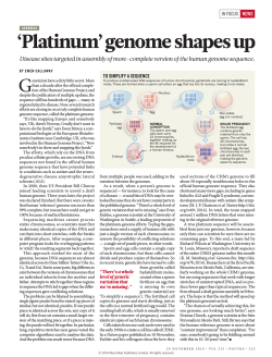

© Copyright 2026