
Price Reactions to Rivals` Local Channel Exits
Price Reactions to Rivals’ Local Channel Exits
ú
Ö. Cem Öztürk
†
Sriram Venkataraman
‡
Pradeep K. Chintagunta
This version: June 2015
Abstract
In this paper, we study the effect of a firm’s local channel exits on prices charged
by incumbents remaining in the marketplace. Exits could result in higher prices due to
tempered competition or lower prices due to reduced co-location or agglomeration benefits. The net effect of these two countervailing forces remains unknown. In addition,
little is known about how this effect could change depending on incumbents’ geographic
locations. We address this research gap by examining new car price reactions by incumbent multi-product automobile dealerships who experience the exit of a Chrysler
dealership in their local markets. We find evidence that the competition effect exceeds
the co-location effect: prices increase by about 1% ($318) following an exit relative to
the price change in the absence of an exit. Importantly, we find that the price increase is
lower at dealerships more proximate to the exiting dealership than dealerships farther
away for the same set of cars available across these locations. This finding suggests
differences in the extent of the two forces (competition and agglomeration) at different distances from the closed dealership. We assess the generalizability of our results
by looking at the impact of GM’s closure of Pontiac dealerships. Taken together, our
results inform consumers, firms, and policymakers about possible implications of an
exit.
Keywords: competitive reaction, market exit, pricing, agglomeration, automobiles,
bailout
ú
Ö. Cem Öztürk is Assistant Professor of Marketing at the Scheller College of Business, Georgia Institute of
Technology. Email: [email protected].
†
Sriram Venkataraman is Assistant Professor of Marketing at the Kenan Flagler Business School, University of
North Carolina - Chapel Hill. Email: [email protected].
‡
Pradeep K. Chintagunta is the Joseph T. and Bernice S. Lewis Distinguished Service Professor of Marketing at
the Booth School of Business at the University of Chicago. Email: [email protected].
The authors thank seminar participants at Emory University, the Marketing Science Conference, and the
Marketing Dynamics Conference, two anonymous Marketing Science reviewers, the associate editor, and the editor
for their insightful comments. This paper has benefited substantially from conversations with professors Sundar
Bharadwaj, Paul Ellickson, Brett Gordon, Wes Hartmann, John Hauser, Ali Hortaçsu, Michael Lewis, Gregor
Matvos, Sanjog Misra, Harikesh Nair, Sridhar Narayanan, Chris Nosko, Ye im Orhun, Jagdish Sheth, K. Sudhir,
Chad Syverson, Necati Tereyagoglu, and Raphael Tomadsen. Chintagunta thanks the Kilts Center for Marketing at
the Booth School of Business for support. All errors are our own. The usual disclaimer applies.
1
Introduction
In this paper, we seek to understand the impact of a firm’s local channel exit on prices charged by
the incumbents that continue to serve the market. When a firm exits the local market, intuition
suggests that the decrease in the number of firms will lead to a less competitive market, and thus
higher prices (the “market power” hypothesis). However, in markets where consumer search costs
are important, firms co-locate with their rivals so as to lower consumer search costs (Rosenthal 1980;
Samuelson and Zhang 1992). In such a setting, exit by a proximate firm could lead to lower prices
as the remaining firms need to compensate for the loss in co-location benefits (the “agglomeration”
hypothesis). In the presence of these two opposing forces, ceteris paribus, the impact of an exit on
prices of surviving incumbents is ambiguous.
Three broad literatures inform us about the price consequences of a change in the number of
firms in a market. The literature on price-concentration and mergers (see Weiss 1989 or Newmark
2004 for a review of these studies) investigates the association between market concentration (measured by the number of firms) and prices. Relying on cross-sectional analyses (either at the market
or firm level), early studies found that concentration is positively associated with prices, but the
presence of unobserved demand and cost shocks could lead to severe biases in their estimated effects
of the number of firms on prices (Bresnahan 1989; Schmalensee 1989; Orhun 2012). More recently,
using firm- or market-level panel data, researchers have been able to account for time-invariant unobservables, and have found no effect of geographic concentration or mergers on retail prices (Davis
2005; Jiménez and Perdiguero 2014). A potential limitation of these panel-data-based studies is
that they rely on aggregate firm-level price indices or investigate industry settings where prices do
not vary within a firm (Cotterill 1986; Manuszak and Moul 2008). Therefore, it is unclear if the
predictions from these studies hold in multi-product firms settings (such as those in the automobile
industry we consider), where prices vary quite significantly within and across firms’ product-lines.
The empirical entry literature also offers inconclusive predictions on the impact of a new competitor on prices (e.g., Simon 2005; Basker and Noel 2009; Ailawadi et al. 2010; Singh et al. 2006;
Gielens et al. 2008; Jia 2008; Singh and Zhu 2008; Zhu and Singh 2009; Zhu et al. 2009; and Zhu
et al. 2011). While several studies have shown incumbent price reductions up to 3% with entry
2
(Basker 2005; Hausman and Leibtag 2007; Basker and Noel 2009), other studies find that no reaction is also common (Ailawadi et al. 2010). Yet, another set of studies finds a positive effect of entry
on prices (Thomas 1999; Yamawaki 2002). At the same time, it is unclear whether the predictions
from this literature translate directly to the case of exits (the focus of our study) due to inherent
differences between entering and exiting firms. For example, consumers with high habit persistence
may not visit a new store that opens in their local market, but they will have to change their
patronage if their favorite store closes (Rhee and Bell 2002). With some notable exceptions, incumbent reactions to exits have received scant attention in the marketing and economics literature.
The studies by Joskow et al. (1994) and Daraban and Fournier (2008) (using market-quarter-level
data) look at exits in the airline industry and show an increase in fares of around 10% following
an exit. The magnitude of competitive reaction to exits in these airline-industry studies is much
higher in absolute terms compared to the findings from entry studies in other industries (Basker
2005; Hausman and Leibtag 2007; Basker and Noel 2009), suggesting that a change in the number
of firms in a market could have a different effect depending on whether the change is due to a
market entry or exit. Since the exit analyses are conducted at the market level, consequences for
individual firms/products are less clear. At the same time, predictions from the analysis of exits in
the airline industry with little spatial differentiation within a market may not directly translate to
industries with potentially high levels of spatial differentiation (e.g., automobile retailing).
A third literature stream, on agglomeration, suggests that firms co-locate to take advantage of
heightened demand (e.g., Marshall 1920; Stahl 1982; Wernerfelt 1994; Vitorino 2012; Datta and
Sudhir 2013). Marshall (1920) makes the observation that consumers are willing to incur substantial
investment of time and travel when buying high-priced products. Thus, he implicitly brings up the
role of consumers’ search costs in stores’ decisions to cluster due to potential demand-side benefits.
Stahl (1982) and Wernerfelt (1994) provided formal models that suggest search costs as a motivation
for firm agglomeration. According to Stahl (1982), a retailer might choose to locate close to its
rivals if increased demand due to co-location (i.e., market area effect) exceeds reduced demand
due to substitution. If the retailer decides to join a cluster of competitors, under high consumer
search costs due to imperfect information, that retailer will enhance the likelihood of visitation for
the other retailers in that location. This positive externality is especially relevant when consumers
3
have limited knowledge related to the characteristics of the products available in different locations.
Wernerfelt (1994), on the other hand, argues that, by locating close to each other, retailers might
commit to a strategy that does not take advantage of consumers’ initial investment. In other words,
retailers can use co-location instead of price advertising especially when consumers need to inspect
the product at the store before purchasing (e.g., consumer durables such as cars). This assertion
could be more applicable for cars as dealers cannot advertise prices for every unit available for sale.
While scholars have examined the impact of these agglomeration benefits on firm entry decisions,
their impact on product-level prices in the context of firm exits has not received much attention.
Taken together, these three streams of literature suggest that in many industries including
automobile retailing, where both the competitive effect and the agglomeration effect are at work,
extant research offers limited to no guidance on how a firm’s exit impacts incumbents’ pricing
decisions. On one hand, Davis (2005) shows that the price effect of competition attenuates with
distance in the motion picture industry. On the other hand, in their analysis of births of new
establishments across six U.S industries, Rosenthal and Strange (2003) find that agglomeration
externalities decline swiftly in the first couple of miles but more gradually after that. Unfortunately,
how the net effect changes with distance is not known.
In this paper, we seek to complement the above literatures in two ways. First, we investigate
how incumbent firms’ product-level pricing decisions respond (direction and magnitude) to a local
competitor’s exit. Second, since competitor exits can result in either gains (due to increased market
power) or losses (due to decreased agglomeration benefits) to incumbent firms, and since these
losses and gains can change with the distance from the exiting firm, we characterize differential
price responses as a function of the geographic distance between the exiting firm and the incumbent.
In order to accomplish these objectives, we compile a unique data set around an important
and unprecedented event in the U.S. automobile retailing industry. In 2009, as part of the much
publicized and debated Federal Troubled Asset Relief Program (TARP), also referred to as the
“automobile industry bailout program,” two of America’s three car manufacturers, i.e., Chrysler
and General Motors (GM), exercised their last-ditch option and filed for Chapter 11 bankruptcy
(Lafontaine and Morton 2010). These were the first auto manufacturer bankruptcies in U.S. history.
The move gave Chrysler the freedom to immediately terminate 789 - or 25% - of its 3,181 dealerships
4
in May 2009, which it completed in the June - July 2009 period (one dealership in our final data
sample closed in August 2009). Such quick and large-scale changes are unparalleled in the U.S.
auto industry, but also afford new opportunities to research distribution-channel-related questions
that were previously not addressable. While our main focus is on the exit of Chrysler dealerships,
we assess the robustness of our results to the closure of GM’s Pontiac dealerships as well.
Specifically, our data and approach provide the following advantages that alleviate the concerns
raised in the context of the previous literature as discussed above. First, due to the extent of
an unprecedented number of Chrysler and GM closings, we observe a large number of exits spanning numerous geographic markets. Second, our data consist of a comprehensive dealer-VIN-level
monthly panel for new cars between October 2008 and September 2010.1 Our unit of analysis
is a “car” as defined by the 10-digit subset of its VIN that reflects most vehicle characteristics.2
We seek to understand how the price of a “car” changes with the exit of a neighboring Chrysler
dealership (relative to the price change in the absence of an exit). Thus, we try to mitigate the
concerns related to the market- or firm-level analysis. Third, while the number of closed Chrysler
dealerships varies across geographic markets, most Chrysler dealerships are terminated in a relatively short period (June-July 2009). So the exit variation in our setting is mainly cross-sectional.
This, combined with the panel structure of the data, allows us to use dealer fixed effects to take
into account strategic selection (if any) of the terminated dealer as well as other dealer-specific
unobservables. Finally, the automobile retailing industry provides an appropriate context to assess
agglomeration-related benefits, as previous studies show that agglomeration effects are particularly
important in industries where product heterogeneity is high and consumers need to personally
inspect goods (Fischer and Harrington 1996; Simon 2005).
We find that retail prices on average increase by 1.006% ($318) following an exit, suggesting
that the overall gains from tempered competition offset a reduction in agglomeration benefits (if
any). To examine if both the “market-power hypothesis” and “agglomeration-benefits hypothesis”
1
A VIN is the abbreviation for a 17-digit vehicle identification number that is used to identify individual motor
vehicles. As discussed later, we define a “car” as every combination of the digits 1-8 and 10-11 of VINs in order
to capture information on most vehicle characteristics. The availability of data at this level allows us to control
for factors such as manufacturer, make, model year, assembly plant, restraint system, body type, engine type, and
transmission.
2
Although we refer to each unit as a “car,” our products span all vehicle types, including convertibles, coupes,
hatchbacks, minivans, sedans, SUVs, trucks and wagons, and all fuel types including gasoline, diesel, hybrid or electric.
5
are at work in our empirical context, we study how prices of cars vary across 3 distance bands
– within 10 miles, between 10 and 20 miles, and between 20 and 30 miles. As there could be
differences in the cars available across these distance bands due to endogenous dealership locations,
we use a subsample of our data including a set of car models that are available across all three
distance bands. For this subsample, we find that the average price increase due to the exit of
Chrysler dealerships within 30 miles is $562. Cars located closest to the exiting dealer (within 10
miles) stand to gain the most from reduced competition, but also experience the most reduction
in demand-side agglomeration benefits, compared to cars at less proximate dealers. As a result,
prices of cars at proximate dealers rise by $265. In contrast, dealers that are located farther away
from the exiting dealer (more than 10 miles) also face tempered competition and do so with limited
to no erosion in agglomeration benefits. This affords distant dealers more room to raise prices
following an exit. For example, cars located at dealers within 10-20 miles (20-30 miles) raise prices
on average by $1,034 ($780) following a Chrysler dealer exit. Since agglomeration benefits erode
much faster than gains from tempered competition, proximate dealers have a lower ability to raise
prices than extremely distant ones ($265 versus $780).
These results have several implications for consumers, firms, and policymakers. For consumers,
our results suggest that if search costs are such that shopping is restricted to the geographic area
where the exit occurs, then going to a dealership closest to the exited dealership will likely yield
the lowest price due to the biggest loss in agglomeration benefits for the nearest dealerships. From
the firm perspective, our results have different implications for product categories in which search
costs may or may not play a role in consumers’ shopping behaviors. In the presence of search costs,
we show that firms need to consider the tradeoffs between competitive and agglomeration effects
when locating retail outlets. Since the exits in our setting were only realized by forced bankruptcy
protection, our findings have direct and immediate appeal to policymakers. First, our findings
inform them on the extent to which prices change as a consequence of the closures. This has
potential implications for consumer welfare and calls for a more complete analysis of the demand
and pricing consequences of the exits. Our findings also inform policymakers of the potential
consequences of relaxing franchise laws if such laws lead to closure of additional dealerships. A
third implication has to do with evaluating the consequences of mergers in such markets. If mergers
6
lead to fewer dealerships, then policymakers need to evaluate not just the competitive effects of
these mergers, but also the consequences for consumers in terms of potentially increasing search
costs due to lower distribution intensity. These implications transcend the auto industry and are
relevant in other forms of retailing where the competitive and agglomeration forces are at play.3
2
Empirical Context
2.1
Background Information: The U.S. Automobile Industry Crisis, Bailout
and Chrysler Dealer Network Consolidation
The automotive industry is an important contributor to the U.S. economy. U.S. auto dealers (new
and used car dealerships) account for 7.9% of total retail employment, directly providing jobs for
an estimated 1.2 million American workers.4 Given its economic significance and rich institutional
features, the automobile industry has had natural appeal to marketing and management scholars.
Academic research examining this industry has generated rich insights around pricing (Bresnahan
1981; Berry et al. 1995; Sudhir 2001), consumer-directed price promotions (Bruce et al. 2006), trade
promotions (Bruce et al. 2005), buyer-supplier links (Martin et al. 1995), channel pass-through
(Busse et al. 2006), information search (Punj and Staelin 1983), leasing versus selling (Desai and
Purohit 1998, 1999), new versus used-car competition (Purohit 1992), consumer-adoption decisions
(Schiraldi 2011), dealer-consumer negotiations (Desai and Purohit 2004), product obsolescence
(Levinthal and Purohit 1989), and hybrid-car adoption (Gallagher and Muehlegger 2011).
However, in the past decade, the Detroit Three have seen their share of the domestic market
drop from 64.5% in 2001 to 47.5% in 2008. The decline in U.S. motor vehicle sales accelerated in
late 2008, with monthly sales running more than 30% lower than the same month the year before.
Americans bought 13.2 million cars and light trucks in 2008, below the 16.1 million units sold in
2007, and well below the peak of the 17.8 million sold in 2000. For the full year, the Detroit Three
were the hardest hit, with 2008 sales falling by 30.3%, 22.7% and 20.3% for Chrysler, GM, and
3
Since we focus on retail prices, our analysis cannot directly speak to either retailer or manufacturer profits or the
long-run survival of bankruptcy-court-protected domestic manufacturers.
4
The employment statistics are based on annual data for 2008 reported by the U.S. Department of Labor, Bureau
of Labor Statistics, Quarterly Census of Employment and Wages (QCEW) program. It includes all employees who
work at automobile dealers included in North American Industry Classification System (NAICS) category 4411 (this
category covers new and used car dealers).
7
Ford, respectively.5 Until 2009, the U.S. was the world’s largest car market, but a recession-led
decline in U.S. sales and a parallel surge in Chinese purchases made China the world’s largest single
auto market. In 2008 alone, the U.S. industry shed 50% of its sales volume and slashed 400K jobs.
Despite declining sales, union contracts severely restricted manufacturers’ ability to shut down
production facilities (SIGTARP 2010), and state franchise laws curtailed them from terminating
their contractual obligations with their downstream channel dealer distribution network (Lafontaine
and Morton 2010). By the end of 2008, GM and Chrysler were unable to secure day-to-day funding
needed to remain in business. On December 19, 2008, President George W. Bush announced a
plan to lend $17.4 billion from the Troubled Asset Relief Program (TARP) to GM and Chrysler
to prevent any near-term bankruptcy and to help them restructure as more viable and competitive
companies over the longer term. GM and Chrysler were advised to use the terms of bankruptcy to
quickly eliminate dealers from their dealer network, an action that the two manufacturers could not
otherwise pursue, given state-level, dealer-leaning franchise laws. As per recommendations from
the U.S. Treasury Department, both Chrysler and GM filed for Chapter 11 bankruptcy protection
on April 30, 2009, and June 1, 2009, respectively. The move gave Chrysler the opportunity to
immediately shut down 789 (or 25%) of its 3,181 dealerships.
Chrysler’s project to consolidate dealerships to sell all three brands under one roof was a major
driver when choosing which dealerships to close. The project was planned to be completed in 2014;
but Chrysler expedited the schedule during the bankruptcy. According to the SIGTARP report:
Chrysler used the following primary criteria to select dealerships to retain or terminate:
whether the dealer’s location was a desirable one targeted by Chrysler; which brands
were offered; the number of new vehicle sales; and the Minimum Sales Responsibility
(“MSR”). Chrysler also considered customer convenience, financial stability of the dealership’s company, condition of the dealership’s buildings and lots, and capacity of the
facility’s buildings and lots. (SIGTARP 2010)
5
Ward’s, Motor Vehicle Facts and Figures, 2009.
8
2.2
Data
The data we analyze come from three sources. Our primary new-car data set, which is provided by a
major marketing research firm, includes dealer/VIN-specific monthly retail prices between October
2008 and September 2010. Apart from retail prices, the data set provides information about dealer
characteristics such as the dealer’s name and address along with vehicle characteristics in each
dealer’s inventory. Vehicle information that we observe include make, model, category (e.g., sedan,
truck, etc.), and model year. Since each vehicle is associated with a unique VIN, we also have
information about the restraint system (e.g., airbags, belts), passenger car identifier, body series
(e.g., trim level, wheel base, number of doors, hardtop, body type, premium/sport), engine type
(e.g., cylinders, displacement, turbo, fuel type), transmission (FWD, AWD, manual/automatic),
and assembly plant. Note that our unit of analysis is not the VIN itself but the limited VIN. This
way we can control for most vehicle characteristics while at the same time pooling across all cars
that share those characteristics.
We complement this primary data set by collecting information on the identities of dealerships
slated for closure using the bankruptcy filings and press releases of Chrysler and GM. This second
data set includes the name, address, and majority owner of each of the closed dealers as well as
the franchises (i.e., brands) carried by each of them.6 Using the addresses of the dealers in our two
data sets, we generate precise latitude and longitude coordinates. Then we compute the distance
in miles from each dealer’s location to each of the closed Chrysler and GM dealers. Accordingly, we
calculate the number of closings within different distance bands (i.e., 0-10 miles, 10-20 miles, and
20-30 miles). Table 1 provides the descriptive statistics for the key variables used in the estimation
procedures as well as the observed car categories in our data set.
Finally, in order to control for the demographic characteristics (e.g., median household income
and population) of local markets, we collected ZIP-code-level demographic information that varies
annually from SimplyMap database (http:// geographicresearch.com/simplymap).
6
A comparison of exit and non-exit dealers of Chrysler across various observable characteristics is provided in
Online Appendix 1.
9
2.2.1
Car Definition and Selection
We define a “car” as every combination of the digits 1-8 and 10-11 of VINs. For instance, for a given
VIN=1FDBP05FXBA100001, our “car” ID is 1FDBP05FBA. The reason for using these digits for
defining cars is that each VIN is composed of several sections. The first three digits identify the
manufacturer, country of origin, and type of vehicle. Digits 4 to 8 identify vehicle attributes such as
engine type, vehicle line, drive type, restraint system, and body type. Digits 10 and 11 identify the
model year and the assembly plant for that vehicle. As such, every combination of the digits 1-8 and
10-11 of VINs provides detailed information about vehicle characteristics. Our limited VIN-based
definition of cars resulted in 4,121 different “cars” associated with 119 different models in our data
set. These 119 models are among the top 150 car models by sales and account for more than 80%
of sales of these 150 models. Note that using the common “make-model-model year” based car
definition results in only 468 different cars. This suggests that the limited VIN-based fixed effects
provide substantially stronger controls for various car characteristics. Our final sample comprises
a total of 437,040 observations, which approximately corresponds to 248 dealers per month, 73
vehicles per dealer/month over a 24-month period.
2.2.2
Retail Market Definition
We use a fixed mileage (i.e., 30 miles) distance radius to define the local retail markets (see, for
example, Ailawadi et al. 2010 and Davis 2005 for a similar approach). In other words, a specific
dealer is assumed to be “treated” by a local market exit if there is a closed dealer within its retail
market. This definition aims at capturing the effect of market exits on dealers that are directly
competing with closed dealers.7 We do not expect significant changes to our results if we enlarge
the retail market coverage because Albuquerque and Bronnenberg (2012) show that the effect of
distance from dealers on consumer utility is marginally decreasing. In other words, most of the
utility reduction happens within short distances. Thus, they find that cross-price elasticities are
negligible when the distance between two dealers is more than 30 miles. While we use the 30-mile
radius to define the market, as we note above, we look for differences across various distance bands,
for a fixed set of car models, within that radius to look at agglomeration versus competition effects.
7
We later conduct a more detailed analysis by breaking up the local market into three distance bands.
10
Based on the above mentioned local market definition, we eliminate dealers that are within the
local market of: i) an inconsistently observed closed Chrysler dealer, ii) a consistently observed
closed Chrysler dealer that switches to another brand after the closing, and iii) a GM dealer that
has been slated for closure. In addition, some of the closed Chrysler dealerships continued to carry
other brands (e.g., Toyota). Although these dealerships appear as incumbent dealerships, they
cannot be designated as rivals to the closed Chrysler dealerships. As our analysis focuses on rival
responses, we excluded such dealerships from our analysis. From the remaining list of dealers, we
dropped those with very few observations (e.g., less than two cars per month) to have a sample of
385 dealers, 69 of which are surviving Chrysler dealerships. Out of these dealers, 60 (14 of which
are Chrysler dealerships) are located in the markets affected by a Chrysler exit (“treated” dealers).8
It is important to note that the closures took place within a small time interval. More precisely,
around 94% of the Chrysler exits within the local market of these affected dealers happened between
June and July 2009. There is only one exit that occurred in August 2009.
A preliminary comparison of the dealers that are affected by Chrysler closures with those
that are not (i.e., control dealers) in the periods before Chrysler closings suggests that these two
groups are relatively similar on various observed characteristics (see Online Appendix 1 for the
comparison statistics). More precisely, the affected and control groups are comparable in terms of
population, average household size, economic stability and percent urban and female population
in the pre-exit period.9 In addition, these dealers have a similar number of makes, models, prices
and categories on average. On the other hand, dealers with Chrysler exits are in markets with
higher income levels, greater white population share, and higher numbers of local competitors.
8
A comparison of the dealerships we finally included in our sample and those we dropped from our sample [because
they met conditions (i) through (iii)] is provided in Online Appendix 1. The difference between included and dropped
dealers is not economically and statistically significant in terms of stability, number of vacant units, percent female
population, or average prices. The difference between the two groups is statistically significant but economically
modest in terms of average household size, average number of makes, average number of models, and average number
of categories. The dropped dealers are different from the included dealers in that they operate in more urban markets
with higher populations, median household incomes and average number of cars sold. This is not unexpected, given
the criteria we used to ensure clean identification. More precisely, we dropped dealers that are within the local
market of: i) an inconsistently observed closed Chrysler dealer, ii) a consistently observed closed Chrysler dealer that
switches to another brand after the closing, and iii) a GM dealer that has been slated for closure. Especially, the third
criterion means that affected dealers that are dropped experienced both Chrysler and GM closings in their market.
In other words, these markets should have had more population to sustain both Chrysler and GM dealerships to start
with compared to the markets where included dealers operate.
9
We report the p-values of the Wilcoxon two-sample test along with the t-test for group differences because the
box plots for the variables (provided in Online Appendix 1) exhibit outliers, thus casting doubt on the distributional
assumption of the t-test.
11
Possibly as a result of being in markets with higher demand potentials, their monthly average sales
are higher than those of control dealers. Using only the pre-closure period monthly time-series
data, we regressed log prices at the car-month-dealer level on the treatment dummy (for all those
dealerships that subsequently saw an exit) along with all the observables that we subsequently use
in our analysis such as population and income at the ZIP-code level, number of local competitors,
etc. and identified unobservable factors reflected in various fixed effects (discussed later). Our
recovered coefficient for the treatment dummy is not significant at the 10% significance level (pvalue of 0.37). This regression result supports the idea that the treatment and control group dealers
are similar in the pre-treatment period after controlling for observables.10
Another issue related to the comparability of treatment and control dealers is the similarity in
terms of local market time trends. Our subsequent analysis explicitly accounts for such trends at
the DMA (where the dealership is located) level via DMA-month fixed effects. However, to assess
whether more micro trends exist, we look at data for ZIP codes in which treatment and control
group dealers are located. Specifically, we report the change in population, employment, household
income, number of vacant units, and stability (% in current residence 5+ years) between 2008
and 2009 in Table 2. The changes in these demographic variables, except for median household
income, show no significant difference between the two groups. Since the data show that household
income increases more in ZIP codes where the treated dealers are located, an increase in price (if
any) associated with cars at these dealerships could be explained by the concomitant increase in
incomes. Consequently, in our subsequent analysis we (i) include this as a control variable, and (ii)
include a dealer-specific time trend in the analysis. In addition, we look at changes in the number
of gas stations and number of electronics and appliance stores in Table 2 to see if there is any
differential trend for businesses related to cars and durable goods. Again the comparison suggests
that the local time trends are not significantly different between control and treatment groups.11
10
We also provide several graphical analyses that show examples of treatment and control group similarity before
treatment as well as differential price changes between the two groups after the treatment in Online Appendix 2.
11
We thank an anonymous reviewer for his/her suggestion.
12
3
Empirical Framework and Identification Strategy
In this section, we assess the effect of local market exits on retail prices. Specifically, we estimate
the impact of the number of Chrysler dealer closings on the retail price of a given car (as defined
previously). Our empirical strategy is closest in spirit to Ailawadi et al. (2010), who examine the
effect of Wal-Mart entry on incumbent retailers’ marketing mix reactions and sales outcomes.
Ideally, given a set of markets with Chrysler dealerships, if we could randomly assign a subset
of markets to a “treatment” condition, i.e., the exit of the Chrysler dealership, and the remaining
to a “control” condition, i.e., no dealer exit, we could then look at the “difference-in-differences”
for prices across the treatment and control groups before and after the Chrysler exit. As Chrysler
likely chooses the treatment strategically rather than randomly, unobserved factors that are correlated with the decision to shut down a Chrysler dealership might also be correlated with, say,
Toyota’s prices; so a simple comparison of prices across rival dealers that do and do not face an
exit may not suffice. Further, one might be concerned about exits that occur for reasons other
than the bankruptcy filing. Two key institutional features help alleviate these concerns. First,
unlike other industry settings where exits are permitted and frequently occurring, federal and state
franchise regulations limit the ability of automobile manufacturers to terminate their franchised
dealerships at will other than via Chapter 11 bankruptcy court protection (Lafontaine and Morton
2010). Therefore, apart from the variation in dealer exits introduced by Chrysler’s dealer network
consolidation event, there is limited additional variation in dealer exits in our setting.12 Second,
while the number of terminated Chrysler dealerships varies across geographic markets, these dealership closings happened (i.e., treatment occurred) largely in the (short) June - July 2009 time frame
across all geographic markets. Note that once a dealership closes, it remains shut – so the treatment
effect on incumbent dealerships is in force from that month on. Hence, much of the exit variation
in our setting is cross-sectional (i.e., varies across geographic markets). Moreover, as we discussed
in subsection 2.1, the selection criteria for Chrysler closings are dealer-specific characteristics. Our
panel data, therefore, allow us to account for strategic selection of the exiting dealer and for other
dealer-specific unobservables, via the inclusion of dealer fixed effects.13
12
13
As we discussed earlier, we exclude markets with GM dealer exits.
Since the timing of exits is the same (up to being either in June or July) across all treated dealerships, the issue
13
The next concern is regarding the market where the exit takes place. In certain states, e.g., Connecticut, Georgia, Michigan and New York, state franchise laws (enacted decades before Chrysler’s
decision to drop dealers) strongly favor automobile dealers at the expense of automobile manufacturers (Smith 1982). Only under bankruptcy court protection can Chrysler override current state
franchise laws, a flexibility not afforded to other non-bankrupt manufacturers. So dealers in certain
states (e.g., “monopoly” states) are more likely to face termination than others.14 Since a dealership can only belong to a particular local geographic market (DMA, e.g., Detroit), our included
dealer fixed effects will also account for these geographic differences. Third, since our analysis is at
the “car” level, differences in dealer reactions for different cars need to be accounted for. For this,
we include car (as previously defined) fixed effects.
Next, given the temporal nature of our data, it is important to control for various trends in prices
that might exist (see Kalnins 2004 and Busse et al. 2006, who discuss the importance of controlling
for trends). We include model/month-year (e.g., Toyota Camry/July 2009), and DMA/monthyear (e.g., Detroit/July 2009) fixed effects in the estimation. Including these fixed effects helps us
control for unobserved factors like manufacturer incentives, advertising, and local gas-price shocks.
For example, demand conditions for cars may change as a result of increasing DMA-level gas prices,
which in turn might affect the pricing policy of the dealers. DMA/month-year fixed effects also
control for differential trends across markets; this effect is identified separately from the treatment
effect since there are multiple dealerships in a given geographic area. Further, if one is concerned
about trends more local to a dealership area (e.g., prices in certain neighborhoods of Detroit change
over time differentially from other neighborhoods), we control for monthly dealer time trends as
well as ZIP-code-level demographics like household income that might change over time (see Table
2).15 Our identifying assumption is that conditional on these controls, dealership closures represent
of strategic timing of exits across dealerships is moot; the absence of a time-varying component of the potentially
endogenous exit decision obviates the concern of any residual endogeneity and the need for instruments. We address
the June versus July exit issue in the robustness checks section of the paper.
14
Model-free evidence does lend support to our ex ante belief about “monopoly” states. Following Smith (1982),
we define a monopoly state as a state where the following policies are in place: i) a manufacturer cannot force dealers
to accept unordered vehicles, ii) franchises cannot be canceled by manufacturers without cause, and iii) there is a
restriction on the entry of new franchises within the exclusive territory of an existing dealer. Only 54% of our dealers
who do not face a Chrysler exit are located in monopoly states, as compared to 85% of the dealers who do experience
a local market Chrysler exit.
15
We thank K. Sudhir for this suggestion. Note that we cannot include dealer/month-year fixed effects since that
is the level of variation of the treatment in our data.
14
an exogenous shock to market structure and consequently, dealership exits are orthogonal to any
residual unobservables in prices. To allay any further concerns regarding endogeneity, we conduct a
“falsification” test; we run our specifications to see whether there is a “treatment” group effect in a
period when there is no closing (i.e., before June 2009). If we were to find a significant impact of this
“placebo treatment” on the outcomes of interest, this would suggest that unobservable differences
that are correlated with Chrysler’s closings are contributing to our estimated effects.
To see if both the competitive and agglomeration effects are at work, we then look at how
prices for a given car (or a set of cars) are affected as the dealership(s) selling that car(s) is (are)
located farther away from the exiting Chrysler dealer—within 10 miles, between 10 and 20 miles,
and between 20 and 30 miles. The idea behind such a comparison is that agglomeration effects and
competitive effects change differentially as one moves farther away from the focal dealership. So a
change in relative effects with distance will be reflected in the prices of the same set of cars across
these distance bands. Further, by focusing on the same car (or set of cars) across the different
distance bands, we alleviate the concern that different car brands might have located differently
relative to one another and the Chrysler dealership (within the 30-mile radius) when opening their
dealerships.
3.1
The Price Model
To evaluate the influence of Chrysler exits on car prices, we regress the natural logarithm of the
retail price for vehicle v at month-year t on the number of Chrysler closings within 30 miles of
the dealer carrying that vehicle (NClosvt ), with the variable taking the value 0 when there is
dealer ), a vector of
no exit, a vector of dummies indicating the dealer that carries the vehicle (Ivt
LimV IN ), a vector
dummies indicating the limited VIN (i.e., specific car type) for the vehicle (Ivt
of dummies denoting car model/month-year-specific fixed effects (Ivt
model/t
denoting DMA/month-year-specific fixed effects (Ivt
DM A/t
), a vector of dummies
), the number of months since the vehicle
was first listed (T SListedvt ), the quadratic term for the number of months since the vehicle was
first listed (T SListed2vt ), ZIP-code-level median household income (ZIP Incvt ), and population
15
(ZIP P opvt ):
ln(P ricevt ) = Ÿ + –NClosvt
+
Õ dealer
d Ivt
+
Õ
LimV IN
LimV IN Ivt
+
model/t
Õ
model/t Ivt
+
DM A/t
Õ
DM A/t Ivt
+⁄1 T SListedvt + ⁄2 T SListed2vt + ’1 ZIP Incvt + ’2 ZIP P opvt + Ávt.
(1)
The coefficient of interest in this specification is –, which represents the average effect of a
one-unit change in Chrysler closings on retail prices.16 In other words, for a one-dealership increase
in the number of closings, we expect to see a 100*[exp(–)-1]% increase in retail price while all other
variables in the model are held constant. Note that if – is small (e.g., less than 0.2, which will be the
case in our estimations), one can say that a one-unit increase in the number of closings will result
in a 100*–% increase in retail price. Dealer fixed effects (
d)
allow us to control for time-invariant
dealer characteristics such as location, size, and chain affiliation. In addition, since the number
of local competitors is very stable during the span of our data set, dealer fixed effects effectively
control for local market structure except for the Chrysler closings (i.e., dealer fixed effects account
for 99% of the variation of the number of local competitors excluding exited Chrysler dealers).17
Limited VIN fixed effects (
LimV IN ),
on the other hand, control for “car”-specific factors such as
manufacturer, brand, model, model year, body type, and trim level, among others. Model/monthyear (
model/t )
and DMA/month-year (
DM A/t )
fixed effects permit us to control for demand
conditions (e.g., popularity of the model, gas prices, etc.), and seasonality, as well as month-yearvarying model- or DMA-level marketing activity (for example, manufacturer promotions to dealers
and consumers18 ). We include the number of months since the vehicle was first listed (⁄1 ) to take
16
Note that the dummy variables and the interaction of them in a usual difference-in-differences specification are
subsumed in the various fixed effects included in Equation 1. Specifically, the treatment dummy in a usual differencein-differences specification is controlled for by our dealer fixed effects, and the after-period dummy is accounted for
by our DMA/month-year fixed effects. The interaction of the treatment dummy and the after-period dummy is
captured by our number-of-closings variable. Thus, the coefficient of the number-of-closings variable (–) shows the
difference-in-differences estimate.
17
Later, we check for robustness to the inclusion of the number of local competitors explicitly in the analysis.
18
Previous literature on manufacturer promotions in the automobile industry suggests that manufacturers usually
make dealer and consumer promotion decisions by nameplate, model, and model year (Busse et al. 2006). We include
model/month-year-level fixed-effects, which will control for the effect of promotions and other unobservables, including
advertising. We also estimated our main specification using model/model year/month-year fixed effects instead of
model/month-year fixed effects. The resulting coefficient for the number-of-closings variable did not change.
16
into account the pressure for the dealer to sell the vehicle. We also include its quadratic term (⁄2 )
to be able to capture a possible curvilinear effect of the number-of-months-since-listed variable on
prices. For example, a significant and positive coefficient for the quadratic term will indicate that
the effect of time-since-listed on retail prices is convex.
As we discussed in subsection 2.2.2, there was a differential change between treatment and
control groups in terms of ZIP-code-level median household income between 2008 and 2009. To
account for such local time-varying demand factors, we control for ZIP-code-level median household
income (’1 ) and population (’2 ), which vary annually.
3.2
Fixed-Effects Estimation Results
Table 3 presents results from eight different fixed-effects specifications where we estimate the effect
of dealer closings on car prices. All eight specifications include dealer, brand, and month-year
fixed effects unless already subsumed by finer fixed effects. Column (1) provides the results from a
specification where we only control for dealer, brand, and month-year fixed effects. We find that the
average effect of a Chrysler dealer closing is significantly negative (-0.581%, i.e., -$184). However,
column (1) also suggests that only 29% of the variation in log prices is explained by the current
specification. In other words, one might worry about potential omitted factors that determine the
log prices of the cars and that may or may not be correlated with our focal closing variable.
Column (2) presents results from the specification where we control for category-specific factors
in addition to the previous controls. The average effect of a closing is a significant reduction in
prices (-0.558%, i.e., -$177). Still, only around 53% of the variation of log prices is accounted for.
Columns (3) through (7) control for additional fixed effects, including model, DMA/monthyear, model/month-year, and car fixed effects, as well as the number of months since the vehicle
was first listed. The results show that as we control for more factors, the average effect of closings
becomes significantly positive and then stays positive, despite some attenuation of the effect. The
inclusion of DMA/month-year fixed effects in column (4) changes the closing coefficient from negative to positive (1.43%, i.e., $454). This can be explained by the fact that a possible DMA-level
decline in the demand for cars that is omitted in column (3) could lead to a downward bias on
the closing coefficient. This might be the case because a decrease in the DMA-level car demand
17
is expected to be positively correlated with competitor closings and negatively correlated with incumbent prices. Therefore, the closing coefficient in column (3) partially reflects the omitted effect
of DMA-level demand shocks. When we further add the time-since-listed variables in our model
(specification 5), we find a significant curvilinear effect of pressure to sell the vehicle (despite a
negligible change in the explanatory power of the model). On the other hand, the inclusion of
model/month-year (specification 6) and car fixed effects (specification 7) suggests an upward bias
on the closing coefficient. This is expected because model/month-year and car fixed effects mainly
control for month-year-varying model popularity and time-invariant product quality, respectively.
The popularity and quality of a car sold by an incumbent is positively correlated with competitor
closings (due to tougher competition) and with price. Thus the omission of these factors will lead
to an upward bias on the closing coefficient, as the positive effect of better incumbent product
quality on price will incorrectly be attributed to competitor closings.
Similarly, our final fixed effect specification shown in column (8) suggests that the omission of
ZIP-code-level median household income and population results in an upward bias on the closing
coefficient. This is because we observe larger increases in household income and population in
ZIP-codes where the treated dealers are located, as we discussed in subsection 2.2.2. Accordingly,
when we omit these variables, their potentially positive effect on prices is attributed to competitor
closings. Thus, our final specification shows that, holding other relevant factors constant, incumbent
dealers increase their prices, on average, by 1.006% in response to a local Chrysler exit.19 This
average effect amounts to an increase of $318 for an average car. This final specification explains
97% of the variation in log prices, which leaves little room for any omitted variables.20
19
We also estimated the specification shown in column (8) using a categorical (instead of continuous) measure for
the number-of-closings variable. The percentage of observations for the 4 categories we observe for the number-ofclosings variable is as follows: no exit - 89%, 1 exit - 9.08%, 2 exits - 1.69%, and 3 exits - 0.24%. Using the no-exit
category as the base category, the coefficients associated with the 3 other category dummies, which are significantly
different from zero, are: 0.76%, i.e., $241 (1 exit), 2.91%, i.e., $921 (2 exits), and 2.69%, i.e., 851 (3 exits). These
results suggest that the marginal effect of an exit for the 1-exit and 2-exit cases (which collectively represent 98% of
the exit observations) are 0.76% ($241) and 1.45% ($460), respectively. As the marginal effect of 1.006% ($318) based
on the continuous measure of the number-of-closings variable summarizes these estimates accurately, the estimation
with the categorical closing variable does not improve the model fit despite estimating more parameters. Thus, we
proceed with the continuous measure of the number-of-closings variable in the rest of the paper.
20
We also checked whether there is any evidence of endogeneity of the exit-timing decision despite the short period
of closings. For the vast majority (87%) of treated dealers, the exits happened either in July, or both in June and July
(i.e., some Chrysler dealers exited a local market in June and others exited the same market in July). So we estimated
the full specification with all controls using only those markets with June-July (July only) exits and controls. The
average closing effect was found to be 1.22%, i.e., $386 (1.50%, i.e., $474). Thus, there is no substantial evidence of
exit-timing endogeneity. We thank Ye im Orhun for this suggestion.
18
3.3
3.3.1
Robustness Checks
Narrow Temporal Windows around Closings
The difference-in-differences approach we took in our fixed-effects estimation uses the prices of cars
that are not affected by dealer closings as the counterfactual prices for cars that are “treated”
by dealer exits. In addition, that approach exploits the entire duration of data (October 2008September 2010) for estimating the average price effect of closings. Although we include a detailed
set of time-varying fixed effects, one concern with this approach is potential unobservable local
market events that might happen in the analysis periods. One way to see if such unobservables
could change our previous result, i.e., a modest positive effect of closings, is to examine the effects
using narrow temporal windows around closings (see Busse et al. 2006 for a similar analysis).21
The idea behind that approach is that as the analysis window around the focal event gets shorter,
the possibility of other events affecting prices is lower. Accordingly, we analyze only observations
within a specific temporal window (e.g., +/-1 month, +/-2 months, etc.) around the closing events.
The underlying assumption here is that the only discontinuous change that affects prices of the
incumbent dealer is the exit of a Chrysler dealership. In addition, analyzing temporally local
treatment effects helps us answer the question of whether our price-reaction results are short-lived.
The effects of closings across various narrow temporal windows are reported in Table 4. They
show that the effect of dealer closings on prices is positive and significant for all of the windows we
consider. So it is unlikely that an unobserved event was the main reason behind our dealer closings
effect.
3.3.2
Differential Trends across Dealers
We already included ZIP-code-level median household income and population that vary annually
in our main specification to account for local time trends. To further check concerns regarding
more granular time trends local to a dealership area (such as the different areas of Detroit example
that we gave before), we estimate another specification where we include dealer/monthly trend
interaction terms to our main specification. Trend interactions are significant for only eight of
21
We thank an anonymous reviewer for his/her suggestion.
19
our analysis dealers. This indicates that dealer and DMA/month-year fixed effects already capture
much of the variation. Accordingly, we re-run the model with only significant dealer/monthly trend
interactions and report the results in column (1) of Table 5. The results show that the treatment
effect is stable (0.961%, i.e., $304), which is consistent with the fact that 97% of the variation in
prices is accounted for using our full fixed effects specification.
3.3.3
Number of Local Competitors
Another potential issue is that the number of local competitors may confound the estimates. For
instance, if Chrysler closed dealerships where the number of local competitors is high and we do
not control for its effect, this could lead to a downward bias on the closing coefficient. This is
because we expect that the number of local competitors is negatively correlated with incumbent
prices. Since DMAs could span a market area much greater than the 30-mile radius around a
focal dealer, our current DMA-month fixed effects specification does not completely control for the
number of local competitors. To see if our results are robust to the inclusion of the number of local
car dealerships in a 30-mile radius of a focal dealer, we collected additional monthly data from R.
L. Polk for the census of local competitors.22 Column (2) in Table 5 reports the results of this
robustness check. When we control for the number of local competitors, we find that the main effect
goes up slightly to 1.019%, or $322 (specification 2 in Table 5), from 1.006%, or $318 (specification
8 in Table 3), showing that the coefficient for the number-of-closings variable is robust. In addition,
the coefficient for the number of local competitors is insignificant. This is because (as we stated
previously) there is not much temporal variation in this measure. Most of the variation in this
measure is cross-sectional and therefore its effect is already subsumed in the dealer fixed effects we
include in our main specification.
3.3.4
Falsification Exercise
To allay any remaining concerns related to endogeneity, we run a “falsification” test. We estimate
our final fixed-effects specification above to see whether there is a “treatment” group effect, i.e.,
placebo effect, in a period when there is no closing (i.e., before June 2009). To do this, we use all
22
We thank the associate editor for his/her suggestion.
20
the pre-exit data and divide that into two halves, namely before and after the placebo treatment.
Then we test whether the placebo-closing effect is significant.
Note that if we were to find a significant impact of the “closing” variable on prices in a period
when no closing happens, this would suggest that unobservable differences that are correlated with
Chrysler closings are contributing to our estimated price effects. The result from the falsification
exercise in Table 5 column (3) shows that the estimate for the placebo-closing variable is insignificant. In other words, the pricing effects are not driven by the correlation of closing variables with
some unobserved shocks that are not controlled for in our final specification. Although in general,
one might attribute such a result to the smaller sample size, it is not an issue here because the
error degrees of freedom is 131,588. Thus, these results further bolster the argument that the price
effects of closings are true closing effects.
The falsification test discussed above also tests the existence of differential trends between treatment and control groups in the pre-treatment period. As a result, the failure to find a significant
coefficient for the placebo-closing variable suggests that the preexisting trends are not different
enough to bias our treatment effect. We also checked if there are differential price trends for control and treatment groups by using the pre-treatment period data and testing an interaction term
between a monthly time trend and a dummy variable for treated units. We find that the estimated
interaction coefficient is very small (0.026% with a p-value of 0.55), supporting the results from the
falsification exercise.
4
Spatial Heterogeneity in Price Effects
The average local market exit effect we find in Section 3 is considerably smaller than the 10%
increase that earlier studies looking at the airline industry have found (Joskow et al. 1994; Daraban
and Fournier 2008). One possible explanation for the small average price increase could be the
magnitude of potential externalities among dealers compared to those among airlines. Specifically,
since the spatial structure of the auto retail market is different from the airline market, the small
effect we find might be a result of averaging among competitors with less spatial differentiation
(those within 10 miles of a closing dealer) and more distant competitors (those within a 20-30-mile
21
distance band from a closing dealer). For example, one could expect that competitors with less
spatial differentiation increase their prices more in response to Chrysler exits than distant competitors. However, if agglomeration benefits erode much faster than gains from spatial spillovers,
then we might find the opposite. Accordingly, in this section, we advance empirical evidence that
both the “market-power hypothesis” and “agglomeration-benefits hypothesis” are indeed at work
in our empirical context.23 To demonstrate this, we estimate a specification where we count the
number of closings within three separate distance bands, namely 0-10 miles, 10-20 miles, and 20-30
miles, representing various levels of spatial differentiation.24 If firms co-locate around their more
substitutable competitors, then firms that are nearest to the closed dealership are most affected by
the competition effect. Intuition suggests that firms in the 0-10 miles band are likely to raise prices
the most, with the effect diminishing as we move away from the focal dealership.
On the other hand, if agglomeration benefits erode as a result of an exit, then the dealerships
located nearest to the closed dealership suffer the most and need to trade off lower prices to
compensate for the increased consumer search costs. As we move farther away from the closed
dealership, those other dealerships do not benefit from the lower search costs as much in the first
place, so they feel less need to keep prices low to attract consumers. In the absence of agglomeration,
only the market power hypothesis will be at work.
What we will see in the data at different distance bands is the net effect of the two forces. Since
the rates at which these two forces erode (as we move farther away from the closed dealership)
could be different, the net effect may not be a monotonic relationship in distance. Specifically, if
going from the first band to the second band agglomeration benefits diminish faster than gains from
reduced competition and if going from the second band to the third band the opposite happens,
then the net effect will be an inverted-U shaped function of the distance from the closed dealership.
As a result, which pattern exists in our data is an empirical question.
To alleviate the concern noted earlier that different cars may be sold in different distance bands,
we use a subset of our original data set that involves a set of car models that are available across all
23
We also investigated other dimensions of heterogeneity such as closed Chrysler dealership size, car popularity
and inventory costs. They indicated small effects on prices (see Online Appendix 3 for details).
24
Davis (2006) and Zhu and Singh (2009) use similar parameterizations to assess the distance-varying impact of
local market structure changes.
22
three distance bands to investigate agglomeration effects. In addition, as we do not have a sufficient
number of surviving Chrysler dealers across the three bands, we drop Chrysler dealers from the
distance-bands analysis. This data set contains 252,375 observations across 44 car models. The
price of an average vehicle is $31,384. The majority of observations are associated with domestic
cars (84.12%), whereas the rest of the observations come from Asian cars (15.88%). The car
categories with the highest number of observations are truck (42.86%), sedan (29.96%), and sport
utility (17.86%). Additional details about this data set are provided in Table 1. The average
increase in car prices across the three distance bands is $562.
The results using the same set of cars across the three distance bands are reported in column (1)
of Table 6. We find that, holding other relevant factors constant, the average increase in prices due
to a local market exit in the primary distance band (0-10 miles) is 0.85% ($265), in the secondary
distance band (10-20 miles) is 3.30% ($1,034), and in the tertiary distance band (20-30 miles) is
2.49% ($780). These findings are in contrast with the intuition that incumbent dealers that are
geographically closer to the exiting Chrysler dealers would benefit more from the lower competition
due to exits, and as a result increase their prices more than their distant surviving peers. However,
our results are consistent with price reactions in an environment where demand-side agglomeration
benefits erode via exits. According to this explanation, proximal dealers might have to cut their
prices in order to offset lost agglomeration efficiencies. Moreover, the lost agglomeration benefits
will affect proximate dealers the most, which is in line with the smallest price increase for incumbents
in the primary distance band. Our results, therefore, reveal a more nuanced effect of market exits
than predicted by either the competition effect or the agglomeration effect on its own.
5
GM Closings
To test the generalizability of our recovered price reaction effects, we investigate, in this section,
the price reactions of surviving dealerships to GM’s bankruptcy-protected local-channel exits.
23
5.1
Data
Our data set for the GM analysis includes dealer/VIN-specific monthly retail prices between October 2008 and September 2010. As GM closed its dealerships in a phased-out manner, there is the
concern that the timing of the closures may be endogenous. In order to alleviate such endogeneity
concerns, we use a subset of GM exits that happened in a relatively short time interval. As there are
a sufficient number of closings in a small time interval for Pontiac dealership closings, we analyze
Pontiac exits between October 2009 and January 2010.
Following the same procedure we used for our Chrysler analysis, we eliminate dealers that
are within the local market of: i) an inconsistently observed closed GM dealer, ii) a consistently
observed closed GM dealer that switches to another brand after the closing, and iii) a Chrysler dealer
that has been slated for closure. From the remaining list of dealers, we dropped closed Pontiac
dealerships that continued to carry other brands and dealerships with very few observations to
have a sample of 265 dealers, 93 of which are surviving GM dealerships. Out of these dealers,
64 (25 of which are GM dealerships) are located in the markets affected by a Pontiac exit. Our
final sample includes 449,987 observations across 3,660 “cars” associated with 98 car models. The
final sample corresponds to 220 dealers per month and 85 cars per dealer/month over a 24-month
period. The bottom half of Table 1 provides the descriptive statistics for the key variables used
in the estimation as well as the observed car categories in our GM analysis data set. Using data
only prior to closures, we ran a regression of log prices on the treatment dummy along with all
the observables. The coefficient for the treatment dummy is not significant at the 10% significance
level, which suggests that, in the case of GM, too, the treatment and control group dealer prices
are similar in the pre-treatment period after controlling for observables.
5.2
Results
Main effect: Table 7 presents results for various fixed-effects specifications that test the effect
of Pontiac dealer closings on car prices. The final specification (8) replicates our main effect
specification for Chrysler. The estimation for that specification shows that incumbent dealers
increase their prices, on average, by 1.472% ($457) in response to a local GM exit. This effect is
24
slightly larger than that for Chrysler analysis (1.006%, or $318), and it suggests that our main
effect result can be extended to the case of GM exits. Similar to the Chrysler case, the final
specification explains around 96% of the variation in log prices. In Table 11 in Online Appendix
3, we report robustness checks regarding differential trends across dealers and the number of local
competitors. These robustness checks show that the exit effect for Pontiac closings does not change
much in response to various additional controls. In addition, the falsification exercise in column
(3) indicates that the placebo-closing variable is insignificant.
Spatial heterogeneity in price effects: For the agglomeration-effects analysis, we used a sample of
our data with a set of car models that we observed across all three distance bands. In addition, we
restricted the sample to competing brands for a meaningful comparison with our Chrysler analysis.
The final sample covers 226,147 observations across 48 car models. The estimated coefficients for
the agglomeration analysis are shown in column (2) of Table 6. The coefficients indicate that the
average increase in prices due to a local Pontiac exit in the primary distance band (0-10 miles) is
1.23% ($395), in the secondary distance band (10-20 miles) is 1.84% ($591), and in the tertiary
distance band (20-30 miles) is 1.39% ($447). Again, we find that the smallest price increase for
incumbent dealers is in the nearest distance band. This result further supports the idea that
agglomeration effect is at work, although the relative differences across bands are smaller in this
case than in the Chrysler situation. In summary, our GM analysis results are qualitatively similar
to our Chrysler analysis findings.
6
Conclusion
Firms use local market exits as a strategic way to cope with significant declines in demand, especially
in times of economic crisis. Given the prevalence of local market exits, it is useful for policymakers
and managers to have a better understanding of the effect of exits on prices, and on product
competition in general. This paper investigates the price effects of Chrysler’s dealer closings in
the U.S. auto industry. Using a unique and extensive auto dealer panel data set on new cars that
includes monthly observations at the dealer/vehicle level, we provide some empirical evidence on
the price effects of local market exits in a setting with durable goods, high product heterogeneity,
25
and a complex spatial market structure.
We find that retail prices on average increase by 1.006% ($318) following an exit, suggesting that
incumbent dealers realize higher pricing power from tempered competition. In order to separate
out the competition and agglomeration effects, we also investigate the spatial heterogeneity of price
reactions. We find that agglomeration benefits erode much faster than gains from tempered competition. Accordingly, proximate dealers (within 10 miles) have an even lower ability to raise prices
than extremely distant (20-30 miles) firms ($265 versus $780). This result supports consumers’
search costs motivation for store clustering put forth by previous agglomeration studies (Marshall
1920; Stahl 1982; Wernerfelt 1994). Our GM analysis suggests that the Chrysler closing results are
qualitatively generalizable to other firm exits. Collectively, our results inform consumers, firms,
and policymakers about possible implications of a firm exit regarding changes in the market power
of incumbent firms and heterogeneous spatial outcomes.
Although this study makes several contributions to the empirical literature on market exits and
distribution channels, it has several limitations. Consistent with the vast majority of the extant
studies on competitive reactions, this study, too, investigates the impact of exits on one aspect
of the marketing mix, i.e., retailer pricing. Expanding the investigation to other elements of the
marketing mix will nicely augment the current study. Our distance-bands analysis shows that the
relationship between the distance from the exiting dealership and price increases due to exits follows
an inverted-U shape. Although this finding indirectly suggests that the inverted-U pattern emerges
as a result of two countervailing forces (i.e., competition and agglomeration), we do not model
these forces explicitly. Our analysis is limited by our data, which contain dealer-vehicle-specific
retail prices. By focusing on these prices, we are able to study the incumbent dealers’ reactions
across their entire inventory. Understanding how dealers’ reactions to Chrysler exits manifest in
transacted prices is another valuable direction of future research inquiry. However, this will come
at the expense of studying price reactions only on a subset of the dealer inventory. Our results
are based on the exits of two firms in a single industry critical to the success of the U.S. economy.
Future research can investigate and contrast similar large-scale distribution channel changes in
other industry settings. In the current study, our distribution channel exits are rooted in the
financial distress of the upstream manufacturer. We also hope that future research will investigate
26
whether and how incumbent retailers differentially respond to market structure changes induced
by the financial distress of the upstream manufacturer versus the financial woes of the downstream
competing retailer.
References
Ailawadi, K.L., J. Zhang, A. Krishna and M.W. Kruger (2010), ‘When Wal-Mart enters: How incumbent retailers react and how this affects their sales outcomes’, Journal of Marketing Research
47(4), 577–593.
Albuquerque, P. and B.J. Bronnenberg (2012), ‘Measuring the impact of negative demand shocks
on car dealer networks’, Marketing Science 31(1), 4–23.
Basker, E. (2005), ‘Selling a cheaper mousetrap: Wal-Mart’s effect on retail prices’, Journal of
Urban Economics 58(2), 203–229.
Basker, E. and M. Noel (2009), ‘The evolving food chain: Competitive effects of Wal-Mart’s entry
into the supermarket industry’, Journal of Economics & Management Strategy 18(4), 977–1009.
Berry, S., J. Levinsohn and A. Pakes (1995), ‘Automobile prices in market equilibrium’, Econometrica 63(4), 841–890.
Bresnahan, T.F. (1981), ‘Departures from marginal-cost pricing in the American automobile industry: Estimates for 1977–1978’, Journal of Econometrics 17(2), 201–227.
Bresnahan, T.F. (1989), ‘Empirical studies of industries with market power’, Handbook of industrial
organization 2, 1011–1057.
Bruce, N., P.S. Desai and R. Staelin (2005), ‘The better they are, the more they give: Trade
promotions of consumer durables’, Journal of Marketing Research 42(1), 54–66.
Bruce, N., P.S. Desai and R. Staelin (2006), ‘Enabling the willing: Consumer rebates for durable
goods’, Marketing Science 25(4), 350–366.
Busse, M., J. Silva-Risso and F. Zettelmeyer (2006), ‘$1,000 cash back: The pass-through of auto
manufacturer promotions’, The American Economic Review 96(4), 1253–1270.
Cotterill, Ronald W. (1986), ‘Market power in the retail food industry: Evidence from Vermont’,
The Review of Economics and Statistics 68(3), 379–386.
Daraban, B. and G.M. Fournier (2008), ‘Incumbent responses to low-cost airline entry and exit: A
spatial autoregressive panel data analysis’, Research in Transportation Economics 24, 15–24.
Datta, S. and K. Sudhir (2013), ‘Does reducing spatial differentiation increase product differentiation? Effects of zoning on retail entry and format variety’, Quantitative Marketing and Economics
11(1), 83–116.
Davis, P. (2005), ‘The effect of local competition on admission prices in the U.S. motion picture
exhibition market’, Journal of Law and Economics 48(2), 677–707.
27
Davis, P. (2006), ‘Spatial competition in retail markets: Movie theaters’, The RAND Journal of
Economics 37(4), 964–982.
Desai, P.S. and D. Purohit (1998), ‘Leasing and selling: Optimal marketing strategies for a durable
goods firm’, Management Science 44(11), 19–34.
Desai, P.S. and D. Purohit (1999), ‘Competition in durable goods markets: The strategic consequences of leasing and selling’, Marketing Science 18(1), 42–58.
Desai, P.S. and D. Purohit (2004), “‘Let me talk to my manager”: Haggling in a competitive
environment’, Marketing Science 23(2), 219–233.
Fischer, J.H. and J.E. Harrington (1996), ‘Product variety and firm agglomeration’, The RAND
Journal of Economics 27(2), 281–309.
Gallagher, K.S. and E. Muehlegger (2011), ‘Giving green to get green? Incentives and consumer
adoption of hybrid vehicle technology’, Journal of Environmental Economics and Management
61(1), 1–15.
Gatignon, H., E. Anderson and K. Helsen (1989), ‘Competitive reactions to market entry: Explaining interfirm differences’, Journal of Marketing Research 26(1), 44–55.
Gielens, K., L.M. Van de Gucht, J. Steenkamp and M.G. Dekimpe (2008), ‘Dancing with a giant: The effect of Wal-Mart’s entry into the United Kingdom on the performance of European
retailers’, Journal of Marketing Research 45(5), 519–534.
Hausman, J. and E. Leibtag (2007), ‘Consumer benefits from increased competition in shopping
outlets: Measuring the effect of Wal-Mart’, Journal of Applied Econometrics 22(7), 1157–1177.
Jia, P. (2008), ‘What happens when Wal-Mart comes to town: An empirical analysis of the discount
retailing industry’, Econometrica 76(6), 1263–1316.
Jiménez, J.L. and J. Perdiguero (2014), ‘Mergers and difference-in-difference estimator: Why firms
do not increase prices?’, European Journal of Law and Economics pp. 1–27.
Joskow, A.S., G.J. Werden and R.L. Johnson (1994), ‘Entry, exit, and performance in airline
markets’, International Journal of Industrial Organization 12(4), 457–471.
Kalnins, A. (2004), ‘An empirical analysis of territorial encroachment within franchised and
company-owned branded chains’, Marketing Science 23(4), 476–489.
Lafontaine, F. and F.S. Morton (2010), ‘Markets: State franchise laws, dealer terminations, and
the auto crisis’, The Journal of Economic Perspectives 24(3), 233–250.
Levinthal, D.A. and D. Purohit (1989), ‘Durable goods and product obsolescence’, Marketing Science 8(1), 35–56.
Manuszak, M.D. and C.C. Moul (2008), ‘Prices and endogenous market structure in Office Supply
superstores’, The Journal of Industrial Economics 68(3), 94–112.
Marshall, A. (1920), Principles of economics, Macmillan, London.
Martin, X., W. Mitchell and A. Swaminathan (1995), ‘Recreating and extending Japanese automobile buyer-supplier links in north America’, Strategic Management Journal 16(8), 589–619.
28
Newmark, C.M. (2004), ‘Price-concentration studies: There you go again’, Available at SSRN
503522 .
Orhun, A.Y. (2012), ‘Spatial differentiation in the supermarket industry: The role of common
information’, Quantitative Marketing and Economics 11(1), 1–35.
Punj, G.N. and R. Staelin (1983), ‘A model of consumer information search behavior for new
automobiles’, Journal of Consumer Research 9(4), 366–80.
Purohit, D. (1992), ‘Exploring the relationship between the markets for new and used durable
goods: The case of automobiles’, Marketing Science 11(2), 154–167.
Rhee, H. and D.R. Bell (2002), ‘The inter-store mobility of supermarket shoppers’, Journal of
Retailing 78(4), 225–237.
Rosenthal, R.W. (1980), ‘A model in which an increase in the number of sellers leads to a higher
price’, Econometrica 48(6), 1575–79.
Rosenthal, S.S. and W.C. Strange (2003), ‘Geography, industrial organization, and agglomeration’,
Review of Economics and Statistics 85(2), 377–393.
Samuelson, L. and J. Zhang (1992), ‘Search costs and prices’, Economics Letters 38(1), 55–60.
Schiraldi, P. (2011), ‘Automobile replacement: A dynamic structural approach’, The RAND journal
of economics 42(2), 266–291.
Schmalensee, R. (1989), ‘Inter-industry studies of structure and performance’, Handbook of industrial organization 2, 951–1009.
SIGTARP (2010), ‘Factors affecting the decisions for General Motors and Chrysler to reduce their
dealership networks’. Washington, D.C., Office of the Special Inspector General.
Simon, D. (2005), ‘Incumbent pricing responses to entry’, Strategic Management Journal
26(13), 1229–1248.
Singh, V., K.T. Hansen and R.C. Blattberg (2006), ‘Market entry and consumer behavior: An
investigation of a Wal-Mart supercenter’, Marketing Science 25(5), 457–476.
Singh, V. and T. Zhu (2008), ‘Pricing and market concentration in oligopoly markets’, Marketing
Science 27(6), 1020–1035.
Smith, R.L. (1982), ‘Franchise regulation: An economic analysis of state restrictions on automobile
distribution’, Journal of Law and Economics 25(1), 125–157.
Stahl, K. (1982), ‘Differentiated products, consumer search, and locational oligopoly’, The Journal
of Industrial Economics 31(1/2), 97–113.
Sudhir, K. (2001), ‘Competitive pricing behavior in the auto market: A structural analysis’, Marketing Science 20(1), 42–60.
Thomas, L.A. (1999), ‘Incumbent firms’ response to entry: Price, advertising, and new product
introduction’, International Journal of Industrial Organization 17(4), 527–555.
Vitorino, M.A. (2012), ‘Empirical entry games with complementarities: An application to the
shopping center industry’, Journal of Marketing Research 49(2), 175–191.
29
Weiss, L.W. (1989), Concentration and price, MIT Press.
Wernerfelt, B. (1994), ‘Selling formats for search goods’, Marketing Science 13(3), 298–309.
Yamawaki, H. (2002), ‘Price reactions to new competition: A study of US luxury car market,
1986–1997’, International Journal of Industrial Organization 20(1), 19–39.
Zhu, T. and V. Singh (2009), ‘Spatial competition with endogenous location choices: An application
to discount retailing’, Quantitative Marketing and Economics 7(1), 1–35.
Zhu, T., V. Singh and A. Dukes (2011), ‘Local competition, entry, and agglomeration’, Quantitative
Marketing and Economics 9(2), 129–154.
Zhu, T., V. Singh and M.D. Manuszak (2009), ‘Market structure and competition in the retail
discount industry’, Journal of Marketing Research 46(4), 453–466.
30
Figure 1: Locations of Treatment and Control Dealers
31
Table 1: Descriptive Statistics
Chrysler estimation data for the main effect of closings
Continuous Variables
N. Obs.
Mean
Std. Dev.
Min
Max
Price (in $U.S.)
437,040
31,723
10,756
7,990
121,130
Time since listed (months)
437,040
3.475
2.803
1
32
ZIP-code-level median household income (in $U.S.)
433,037
44,842
9,714
21,254
90,148
ZIP-code-level population
433,037
20,752
11,288
814
74,902
Number of closings within 30 miles
437,040
0.131
0.402
0
3
Categorical Variables (Percentage Occurrence)
Category: Convertible (0.25), Coupe (4.13), Hatchback (3.03), Sedan (30.23), SUV (21.20), Truck (36.83),
Van (2.58), Wagon (1.75). Country/region of origin: Domestic (70.83; Chrysler 7.78), Asian (28.80), European (0.37).
Chrysler estimation data for spatial heterogeneity in price effects
Continuous Variables
N. Obs.
Mean
Std. Dev.
Min
Max
Price (in $U.S.)
252,375
31,384
10,594
7,990
98,540
Time since listed (months)
252,375
3.532
2.801
1
29
ZIP-code-level median household income (in $U.S.)
252,375
45,120
9,484
21,254
75,103
ZIP-code-level population
252,375
19,270
10,882
814
74,902
Number of closings within the primary distance band
252,375
0.064
0.259
0
2
Number of closings within the secondary distance band
252,375
0.011
0.104
0
1
Number of closings within the tertiary distance band
252,375
0.047
0.234
0
2
Categorical Variables (Percentage Occurrence)
Category: Convertible (0.27), Coupe (5.38), Hatchback (1.54), Sedan (29.96), SUV(17.86), Truck (42.86),
Wagon (2.14). Country/region of origin: Domestic (84.12), Asian (15.88).
GM estimation data for the main effect of closings
Continuous Variables
N. Obs.
Mean
Std. Dev.
Min
Max
Price (in $U.S.)
449,987
31,063
10,606
7,990
149,900
Time since listed (months)
449,987
3.628
2.879
1
32
ZIP-code-level median household income (in $U.S.)
449,987
46,320
10,494
24,819
81,489
ZIP-code-level population
449,987
19,699
11,819
1,263
58,175
Number of closings within 30 miles
449,987
0.172
0.487
0
3
Categorical Variables (Percentage Occurrence)
Category: Convertible (0.24), Coupe (4.91), Hatchback (3.98), Sedan (27.31), SUV (20.55), Truck (37.37),
Van (3.77), Wagon (1.86). Country/region of origin: Domestic (72.84; GM 29.96), Asian (27.16).
GM estimation data for spatial heterogeneity in price effects
Continuous Variables
N. Obs.
Mean
Std. Dev.
Min
Max
Price (in $U.S.)
226,147
32,141
10,431
8,340
103,075
Time since listed (months)
226,147
3.684
2.835
1
26
ZIP-code-level median household income (in $U.S.)
226,147
46,794
11,048
24,819
81,489
ZIP-code-level population
226,147
19,097
11,928
1,263
58,175
Number of closings within the primary distance band
226,147
0.093
0.337
0
2
Number of closings within the secondary distance band
226,147
0.049
0.216
0
1
Number of closings within the tertiary distance band
226,147
0.043
0.244
0
3
Categorical Variables (Percentage Occurrence)
Category: Convertible (0.35), Coupe (4.82), Hatchback (3.61), Sedan (19.97), SUV(22.38), Truck (43.98),
Van (4.41), Wagon (0.49). Country/region of origin: Domestic (85.32), Asian (14.68).
32
Table 2: Local Market Trends: Treatment versus Control Dealer Comparison
Change between 2008
Control
and 2009
Mean
Treatment
Std. Dev.
Mean
Differences
Std. Dev.
Control Mean
Wilcoxon
minus Treatment
Two-Sample
Mean
Test p-value
Population
-28.328
2,003
61,513
486
-89.840
0.479
Total Civilian Employment
-266.1
908.4
-229.2
260.1
-36.943
0.778
3.585
9.242
5.851
6.520
-2.266*
0.083
-20.127
185.6
-29.333
74.470
9.207
0.115
-0.012
0.444
-0.080
0.814
0.068
0.601
0.061
1.844
0.256
1.094
-0.195
0.273
-0.096
1.108
-0.205
0.923
0.109
0.275
% Median Household
Income
Number of Vacant Units
Stability (% in current
residence 5+ years)
Number of Gas Stations
Number of Electronics &
Appliance Stores
*p<0.10; ** p<0.05; ***p<0.01. Notes: Demographic variables show ZIP-code-level census data with N (control) = 229 and
N (treatment) = 39.
Table 3: Fixed-Effects Estimation: The Impact of Chrysler Closings on ln(P rice)
Variable
Number of closings
within 30 miles
(1)
(2)
(3)
(4)
(5)
(6)
(7)
(8)
-0.581***
-0.558***
-0.420***
1.430***
1.404***
1.037***
1.083***
1.006***
(0.214)
(0.175)
(0.105)
(0.201)
(0.201)
(0.206)
(0.093)
(0.093)
Time since listed
-
-
-
-
-0.683***
-0.686***
-0.231***
-0.230***
(0.020)
(0.021)
(0.010)
(0.010)
Time since listed2
-
-
-
-
0.026***
0.029***
0.007***
0.007***
(0.002)
(0.002)
(0.001)
(0.001)
ZIP-code-level
-
-
-
-
-
-
-
0.144***
median household
(0.015)
income
ZIP-code-level
-
-
-
-
-
-
-
Category fixed effects
No
Yes
Yes
Yes
Yes
Yes
Yes
Yes
Model fixed effects
No
No
Yes
Yes
Yes
Yes
Yes
Yes
DMA/month-year
No
No
No
Yes
Yes
Yes
Yes
Yes
No
No
No
No
No
Yes
Yes
Yes
population
0.412***
(0.066)
fixed effects
Model/month-year
fixed effects
Car fixed effects
Adjusted R2
No
No
No
No
No
No
Yes
Yes
0.292
0.526
0.831
0.834
0.834
0.837
0.968
0.968
*p<0.10; ** p<0.05; ***p<0.01. Notes: All estimations include dealer, brand, and month-year fixed effects unless already
subsumed by finer fixed effects. Estimations for columns (1)–(7) are based on 437,040 observations across 119 car models. The
estimation for column (8) uses 433,037 observations since median household income and population data are not available for
some ZIP codes. All coefficients and standard errors are scaled up by a factor of 100. Standard errors are given in parentheses.
Similar estimations with robust standard errors did not change the results given the very large number of observations used in
the estimations.
33
Table 4: Narrow Temporal Windows around Closings
Variable
Number of closings within 30 miles
Time since listed
Time since
listed2
1-Month
2-Month
3-Month
5-Month
7-Month
Window
Window
Window
Window
Window
0.483*
0.698***
0.634***
0.792***
1.110***
(0.289)
(0.211)
(0.180)
(0.143)
(0.123)
-0.302***
-0.317***
-0.331***
-0.344***
-0.331***
(0.030)
(0.024)
(0.021)
(0.017)
(0.014)
0.010***
-0.001
0.002
0.005***
0.009***
(0.003)
(0.002)
(0.002)
(0.001)
(0.001)
n/a
n/a
n/a
0.279***
0.174***
ZIP-code-level population
n/a
n/a
n/a
DMA/month-year fixed effects
Yes
Yes
Yes
Model/month-year fixed effects
Yes
Yes
Car fixed effects
Yes
Yes
ZIP-code-level median household
income
Dealer fixed effects
(0.028)
(0.017)
0.239
0.772***
(0.199)
(0.092)
Yes
Yes
Yes
Yes
Yes
Yes
Yes
Yes
Yes
Yes
Yes
Yes
Yes
Adjusted R2
0.971
0.970
0.970
0.969
0.968
Number of observations
74,295
105,287
136,784
205,929
274,982
*p<0.10; ** p<0.05; ***p<0.01. Notes: All coefficients and standard errors are scaled up by a factor of 100. Standard errors
are given in parentheses. ZIP-code-level median household income and population vary annually, so they are not identified in
the first three columns where we have only observations in 2009.
Table 5: Robustness Checks
Variable
Number of closings within 30 miles
Time since listed
Time since listed2
ZIP-code-level median household income
ZIP-code-level population
Number of local competitors
Adjusted R2
(1) Trend
(2) Number of Local
Interactions
Competitors
0.961***
1.019***
(3) Falsification
0.318
(0.093)
(0.094)
(0.206)
-0.225***
-0.230***
-0.429***
(0.010)
(0.010)
(0.025)
0.007***
0.007***
0.012***
(0.001)
(0.001)
(0.002)
0.151***
0.145***
0.193***
(0.015)
(0.015)
(0.020)
0.449***
0.415***
0.892***
(0.066)
(0.066)
(0.126)
0.968
-0.031
0.140
(0.033)
(0.134)
0.968
0.967
*p<0.10; ** p<0.05; ***p<0.01. Notes: All coefficients and standard errors are scaled up by a factor of 100. The dependent
variable in all estimations is ln(Price). Estimations for columns (1) and (2) use 433,037 observations. The estimation in column
(3) is based only on pre-closings period (135,424 observations) to run a falsification test with a placebo treatment variable.
Standard errors are given in parentheses. Similar estimations with robust standard errors did not change the results given
the very large number of observations used in the estimations. All estimations include dealer, car, DMA/month-year and
model/month-year fixed effects. Specification in column (1) additionally includes significant dealer/monthly trend interactions.
34
Table 6: Spatial Heterogeneity in Price Effects - Competing Brands
(1) Chrysler Closings
(2) GM Closings
Number of closings within the 0-10 miles band
0.845*** (0.263)
1.229*** (0.124)
Number of closings within the 10-20 miles band
3.295*** (0.581)
1.836***(0.195)
Number of closings within the 20-30 miles band
2.485*** (0.252)
1.394*** (0.205)
Time since listed
-0.266*** (0.014)
-0.252*** (0.017)
Time since listed2
0.010*** (0.001)
0.008*** (0.001)
ZIP-code-level median household income
Variable
0.112*** (0.024)
-0.030 (0.023)
ZIP-code-level population
-0.169* (0.100)
-0.549*** (0.071)
Number of local competitors
-0.062 (0.053)
-0.148** (0.062)
0.965
0.951
Adjusted R2
*p<0.10; ** p<0.05; ***p<0.01. Notes: All coefficients and standard errors are scaled up by a factor of 100. The dependent
variable in all estimations is ln(Price). Estimations for column (1) are based on 252,375 observations. Estimations for column
(2) are based on 226,147 observations. Similar estimations with robust standard errors did not change the results given the very
large number of observations used in the estimations. All estimations include dealer, car, DMA/month-year and model/monthyear fixed effects as well as significant dealer/monthly trend interactions.
Table 7: Fixed-Effects Estimation: The Impact of GM (Pontiac) Closings on ln(P rice)
Variable
Number of closings
within 30 miles
(1)
(2)
(3)
(4)
(5)
(6)
(7)
(8)
1.121***
1.069***
0.971***
1.683***
1.603***
1.547***
1.304***
1.472***
(0.131)
(0.107)
(0.064)
(0.126)
(0.125)
(0.127)
(0.059)
(0.061)
Time since listed
-
-
-
-
-0.655***
-0.669***
-0.249***
-0.248***
(0.021)
(0.021)
(0.010)
(0.010)
Time since listed2
-
-
-
-
0.026***
0.030***
0.007***
0.007***
(0.002)
(0.002)
(0.001)
(0.001)
ZIP-code-level median
-
-
-
-
-
-
-
household income
ZIP-code-level
0.019
(0.015)
-
-
-
-
-
-
-
population
-0.513***
(0.038)
Category fixed effects
No
Yes
Yes
Yes
Yes
Yes
Yes
Yes
Model fixed effects
No
No
Yes
Yes
Yes
Yes
Yes
Yes
DMA/month-year fixed
No
No
No
Yes
Yes
Yes
Yes
Yes
No
No
No
No
No
Yes
Yes
Yes
No
No
No
No
No
No
Yes
Yes
0.215
0.481
0.814
0.816
0.817
0.820
0.962
0.962
effects
Model/month-year fixed
effects
Car fixed effects
Adjusted
R2
*p<0.10; ** p<0.05; ***p<0.01. Notes: All estimations include dealer, brand, and month-year fixed effects unless already
subsumed by finer fixed effects. Estimations are based on 449,987 observations across 98 car models. All coefficients and
standard errors are scaled up by a factor of 100. Standard errors are given in parentheses.
35
Online Appendix 1: Additional Tables and Figures
In this appendix, we provide the additional figures and tables mentioned in the paper.
Figure 2: Treatment versus Control Dealer Comparison - 1
36
Figure 3: Treatment versus Control Dealer Comparison - 2
37
38
Note that the total number of observations used for generating the density graphs is as follows: Ford - 644 (48 for the treatment group with 1 closing and 12 for the treatment
group with 2 closings); Toyota - 265 (29 for the treatment group with 1 closing and 15 for the treatment group with 2 closings); Honda - 62 (24 for the treatment group with 1
closing.).
Figure 4: Average Price Distribution for Control and Treated Dealers by Brand and Number of Exits
Table 8: Summary Statistics: Treatment versus Control Dealer Comparison
Variables
Control
Mean
Std. Dev.
Treatment
Mean
Std. Dev.
Differences
Control Mean
Wilcoxon
minus Treatment
Two-Sample
Mean
Test p-value
Population
16,366
11,240
17,964
11,410
-1,598
0.434
Median Household Income
40,983
8,164
47,631
10,399
-6,648***
<0.001
Average Household Size
2.405
0.310
2.348
0.209
0.057
0.333
Stability
34.709
8.070
37.218
7.735
-2.509*
0.138
Number of Vacant Units
851.6
1,126
626.4
527.7
225.2**
0.183
Percent White Population
82.738
16.377
88.192
11.252
-5.454**
0.061
Percent Urban Population
57.299
27.386
63.276
29.832
-5.976
0.084
Percent Female Population
50.278
2.263
50.915
1.487
-0.637**
0.185
Proportion Belonging to
53.71%
Monopoly States
84.62%
Average Number of Makes
2.882
2.658
2.921
1.781
Average Number of Models
19.992
10.287
19.895
Average Price
31,265
6,152
29,655
5.948
1.498
14.433
Average Number of
Categories
Average Number of Cars
Sold
Number of Local Chrysler
Competitors
Number of Local
Non-Chrysler Competitors
‰2 test p-value = 0.0003
-0.039
0.966
9.632
0.097
0.636
4,740
1,610*
0.120
6.260
1.584
-0.312
0.094
10.238
20.843
15.341
-6.410**
0.006
2.209
1.620
3.369
2.172
-1.160***
0.003
6.645
5.582
11.199
6.815
-4.554***
<0.001
*p<0.10; ** p<0.05; ***p<0.01. Notes: Demographic variables show ZIP-code level 2008 census data with N (control) = 229
and N (treatment) = 39. Dealer data represent averages of monthly observations prior to Chrysler exits with N (control) = 239
and N (treatment) = 41.
39
Table 9: Summary Statistics: Exit versus Non-Exit Dealer Comparison
Variables
Population
Median Household
Income
Average Household Size
Stability
Number of Vacant Units
Percent White Population
Percent Urban
Population
Percent Female
Population
Proportion Belonging to
Monopoly States
Average Number of
Makes
Average Number of
Models
Average Price
Average Number of
Categories
Average Number of Cars
Sold
Non-Exit
Mean Std. Dev.
Mean
18,189
10,416
28,430
9,826
44,010
8,967
47,906
9,767
-3,897*
0.071
2.391
35.350
736.6
83.673
0.278
8.641
721.6
14
2.305
37.634
979.9
84.464
0.281
6.536
579
10.758
0.085
-2.284
-243.3
-0.791
0.054
0.285
0.018
0.722
60.922
24.793
81.286
14.074
-20.364***
0.0002
50.624
1.725
51.512
1.008
-0.888***
0.017
58.08%
Exit
Std. Dev.
78.95%
Differences
Non-Exit
Wilcoxon
Mean
Twominus Exit
Sample
Mean
Test
p-value
-10,241***
0.001
‰2 test p-value = 0.076
2.644
0.674
1.586
0.764
1.059***
<0.001
15.764
6.319
8.599
5.106
7.166***
<0.001
30,937
5,458
28,182
2,635
2,755***
0.017
5.422
1.560
3.263
2.397
2.159***
<0.001
17.444
25.863
10.105
8.269
7.339***
0.072
*p<0.10; ** p<0.05; ***p<0.01.
Notes: Demographic variables show 2008 census data with N (non-exit) = 198 and N (exit) = 19. Dealer data represent
averages of monthly observations prior to Chrysler exits with N (non-exit) = 220 and N (exit) = 19. For dealer price data we
have N (non-exit) = 177 and N (exit) = 17.
40
Table 10: Affected Dealer Comparison: Included versus Dropped Dealers
Variables
Population
Median Household
Income
Average Household Size
Stability
Number of Vacant Units
Percent White Population
Percent Urban
Population
Percent Female
Population
Proportion Belonging to
Monopoly States
Average Number of
Makes
Average Number of
Models
Average Price
Average Number of
Categories
Average Number of Cars
Sold
Dropped
Included
Mean
Std. Dev.
Mean
Std. Dev.
27,196
16,343
17,964
11,410
Differences
Dropped
Wilcoxon
Mean
Twominus
Sample
Included
Test
Mean
p-value
9,232
0.0003
60,515
20,852
47,631
10,399
12,884***
<0.0001
2.481
37.184
637.4
78.674
0.323
9.760
619.1
19.504
2.348
37.218
626.4
88.192
0.209
7.735
527.7
11.252
0.133***
-0.034
11.044
-9.518***
0.003
0.798
0.822
0.0005
84.588
23.827
63.276
29.832
21.313***
<0.0001
50.852
1.997
50.915
1.487
-0.0633
0.923
56.82%
84.62%
‰2 test p-value = 0.0005
1.694
1.045
2.921
1.781
-1.227***
<0.0001
15.107
8.052
19.895
9.632
-4.788***
<0.0001
33,187
12,463
29,655
4,740
3,531***
0.784
5.708
1.725
6.260
1.584
-0.552**
0.023
34.803
27.657
20.843
15.341
13.960***
0.0008
*p<0.10; ** p<0.05; ***p<0.01.
Notes: Demographic variables show 2008 census data with N (dropped) = 2,302 and N (included) = 39. Dealer data represent
averages of monthly observations prior to Chrysler exits with N (dropped) = 3,235 and N (included) = 41.
41
Online Appendix 2: Graphical Analysis of Retail Prices
In this appendix, we present some preliminary graphical analyses that give us a rough idea of the
impact of market exits on prices. More precisely, we create density plots of the difference in real
prices25 before and after dealer closings of a particular car model for dealerships in the treatment
and control groups. The idea here is to see whether there is any differential change in market prices
between the affected and unaffected dealers. For instance, if the density plot for the control group
is centered around zero and that for the treatment group is centered around a different value, this
would imply that dealer closings could have an effect on market prices. Of course, this implication
is based on the assumption that control group dealers can credibly serve as controls for treatment
dealers. In subsection 2.2.2, we mentioned that the treatment and control group dealerships are
comparable in terms of many market-related observables such as population and average household
size in the period before Chrysler exits. In order to further check the appropriateness of our control
group dealers, we also plot average price distributions for treatment and control group dealers in a
period before closings (i.e., January 2009).
Figure 5 illustrates these plots for two car models. For both of the car models, the plots
showing average price distributions in January 2009 suggest that there is not much difference in
the location of price distributions between treatment and control dealers before the treatment.26
However, for Toyota Tundra, the plots showing the difference in real prices before and after closings
indicate that treatment group dealers cut their prices more than control group dealers after the
closings. In contrast, for Ford Ranger, treatment group dealers raised their prices more than control
group dealers after the closings. In our empirical analysis, we are interested in the average of these
differential changes across all 119 car models. As a result, the direction of the average effect and the
differences in this effect for different sets of cars and distances are empirical questions. Note that the
before-after price differences are calculated for each dealer/model combination separately, meaning
that dealer- and model-level time-invariant factors are already controlled for in these graphs. On
25
We use the Consumer Price Index to convert prices to January 2008 prices for the graphical analysis. In the
sections where we estimate formal models, the natural logarithm of nominal prices is used as the dependent variable,
and we include month-year fixed effects to use only within-month variation in prices.
26
Some treated dealers in our data face more than one Chrysler exit. A graphical comparison of the pre-exit price
distributions for different number of exits is provided in Online Appendix 1. The graphs suggest that the pre-exit
price distributions are similar for different number of closings.
42
the other hand, price difference plots for the two models suggest that there might be model-level
time-varying factors that we should take into account, because control group means are positive
and they are not centered around zero. Therefore, we should assess the difference in the treatment
group using a before-and-after-with-control group (i.e., difference-in-differences) approach.
Since the number of treatment group observations in the model-level density plots is limited, we
pool the observations for the same brand to see whether differential price changes remain between
the affected and control dealers. The patterns become less clear for certain brands such as Ford (see
Figure 6). Although the above graphical analyses provide some preliminary evidence that there is
a differential movement in prices for the dealers of rival brands that are in the same local markets
with closed Chrysler dealers, many confounding factors could affect such a movement. Further,
separating out agglomeration and competition effects is challenging with such an analysis. In order
to be able to control for various confounding factors while measuring the effect of local market
exits, we consider a formal empirical specification in Section 3.
43
44
Note that the total number of observations used for generating the difference density graphs is as follows: Ford Ranger - 42 (4 for the treatment group); Toyota Tundra - 15 (3
for the treatment group). The following steps were employed in creating the price difference density plots: First, for each dealer/model combination in the data set we calculate
average prices (across VINs) one month before and one month after the closings. Second, for each dealer/model combination, we compute the difference between these averages.
Third, we create kernel density plots for the focal model (e.g., Ford Ranger) separately for treatment and control group dealers.
Figure 5: Movement in Prices for Treated Dealers: Examples at the Model Level
45
Note that the total number of dealer/model observations used for generating the difference density graphs is 574 for Ford (64 for the treatment group), 197 for Toyota (39 for
the treatment group), and 89 for Honda (33 for the treatment group).
Figure 6: Movement in Prices for Treated Dealers: Examples at the Brand Level
Online Appendix 3: Additional Robustness
Other Dimensions of Heterogeneity: Closed Chrysler Dealership Size, Car Popularity, and Inventory Costs
We also examined heterogeneous price effects based on the size of the Chrysler dealership closing as
well as the popularity of the car model that is affected by Chrysler closings. More precisely, the size
of the closed Chrysler dealership, measured by the average monthly sales before the closing, captures
the value of the abandoned market for incumbents. For example, the increase in incumbent prices
due to exit could be higher if the closed Chrysler dealership had a larger market (e.g., Gatignon et al.
1989). Similarly, the increase in incumbent prices could depend on the popularity of the car model,
measured by the average monthly sales rank in the pre-closings period. Such heterogeneity might
exist, for instance, if incumbents use Chrysler dealer closings as an opportunity to de-emphasize
relatively unpopular car models. Our results related to these other dimensions of heterogeneity
indicated small effects on prices.
In addition, we assessed the impact of a potential reduction in inventory costs for incumbents
as a result of Chrysler exits. We visually inspected the plots of the average number of months
to sell a vehicle by dealer for treatment and control group dealers. The plots (see below) do not
suggest a differential change between the selling spells between the treatment and control group
dealers. We also formally tested this by regressing the average number of months to sell a vehicle
by dealer on the treatment dummy, an after-period dummy indicating the periods following an exit
and the interaction of the two. The coefficient estimates (standard errors) for these three variables
are -0.360 (0.307), -0.659 (0.157), and 0.043 (0.401), respectively. These results suggest that the
interaction coefficient is insignificant at the 10% level. Hence, we conclude that a reduction in
inventory costs does not change our results. In summary, our core results are robust.
46
Figure 7: Average Number of Months to Sell by Dealer
Additional Robustness Checks for GM Analysis
Table 11: Robustness Checks - GM (Pontiac) Closings
Variable
Number of closings within 30 miles
Time since listed
Time since listed2
ZIP-code-level median household income
ZIP-code-level population
(1) Trend
(2) Number of
Interactions
Local Competitors
1.654***
0.079
(0.061)
(0.063)
(0.131)
-0.250***
-0.248***
-0.314***
(0.010)
(0.010)
(0.018)
0.007***
0.007***
0.009***
(0.001)
(0.001)
(0.002)
0.009
0.052***
-0.042**
(0.015)
(0.015)
(0.018)
-0.488***
-0.600***
0.634***
(0.038)
(0.038)
(0.079)
-0.528***
-0.355***
(0.032)
(0.076)
0.962
0.964
-
Number of local competitors
Adjusted
1.154***
(3) Falsification
R2
0.962
*p<0.10; ** p<0.05; ***p<0.01. Notes: All coefficients and standard errors are scaled up by a factor of 100. The dependent
variable in all estimations is ln(Price). Estimations for columns (1)–(2) use 449,621 observations. The estimation in column
(3) is based only on pre-closings period (211,656 observations) to run a falsification test with a placebo treatment variable.
Standard errors are given in parentheses. All estimations include dealer, car, DMA/month-year and model/month-year fixed
effects. Specification in column (1) additionally includes significant dealer/monthly trend interactions.
47


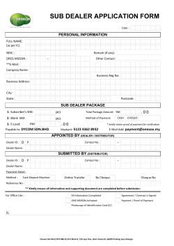


© Copyright 2026