1. technology and computing
2. electronic components

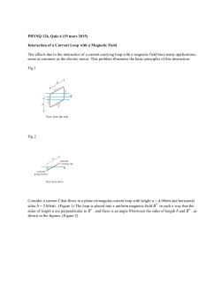
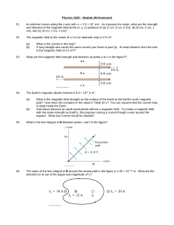
11
Magnetic Circuits
11.1
INTRODUCTION
Magnetism plays an integral part in almost every electrical device used
today in industry, research, or the home. Generators, motors, transformers, circuit breakers, televisions, computers, tape recorders, and
telephones all employ magnetic effects to perform a variety of important tasks.
The compass, used by Chinese sailors as early as the second century
A.D., relies on a permanent magnet for indicating direction. The permanent magnet is made of a material, such as steel or iron, that will
remain magnetized for long periods of time without the need for an
external source of energy.
In 1820, the Danish physicist Hans Christian Oersted discovered
that the needle of a compass would deflect if brought near a currentcarrying conductor. For the first time it was demonstrated that electricity and magnetism were related, and in the same year the French
physicist André-Marie Ampère performed experiments in this area and
developed what is presently known as Ampère’s circuital law. In subsequent years, men such as Michael Faraday, Karl Friedrich Gauss,
and James Clerk Maxwell continued to experiment in this area and
developed many of the basic concepts of electromagnetism—magnetic effects induced by the flow of charge, or current.
There is a great deal of similarity between the analyses of electric
circuits and magnetic circuits. This will be demonstrated later in this
chapter when we compare the basic equations and methods used to
solve magnetic circuits with those used for electric circuits.
Difficulty in understanding methods used with magnetic circuits will
often arise in simply learning to use the proper set of units, not because
of the equations themselves. The problem exists because three different
systems of units are still used in the industry. To the extent practical, SI
will be used throughout this chapter. For the CGS and English systems,
a conversion table is provided in Appendix F.
436

MAGNETIC CIRCUITS
11.2
Same area
Flux lines
b
S
a
N
FIG. 11.1
Flux distribution for a permanent magnet.
N
S
N
S
FIG. 11.2
Flux distribution for two adjacent, opposite
poles.
MAGNETIC FIELDS
In the region surrounding a permanent magnet there exists a magnetic
field, which can be represented by magnetic flux lines similar to electric flux lines. Magnetic flux lines, however, do not have origins or terminating points as do electric flux lines but exist in continuous loops, as
shown in Fig. 11.1. The symbol for magnetic flux is the Greek letter (phi).
The magnetic flux lines radiate from the north pole to the south pole,
returning to the north pole through the metallic bar. Note the equal
spacing between the flux lines within the core and the symmetric distribution outside the magnetic material. These are additional properties of
magnetic flux lines in homogeneous materials (that is, materials having
uniform structure or composition throughout). It is also important to
realize that the continuous magnetic flux line will strive to occupy as
small an area as possible. This will result in magnetic flux lines of minimum length between the like poles, as shown in Fig. 11.2. The strength
of a magnetic field in a particular region is directly related to the density of flux lines in that region. In Fig. 11.1, for example, the magnetic
field strength at a is twice that at b since twice as many magnetic flux
lines are associated with the perpendicular plane at a than at b. Recall
from childhood experiments that the strength of permanent magnets
was always stronger near the poles.
If unlike poles of two permanent magnets are brought together, the
magnets will attract, and the flux distribution will be as shown in Fig.
11.2. If like poles are brought together, the magnets will repel, and the
flux distribution will be as shown in Fig. 11.3.
Flux lines
S
Soft iron
N
N
N
S
S
Glass
FIG. 11.3
Flux distribution for two adjacent, like poles.
FIG. 11.4
Effect of a ferromagnetic sample on the flux
distribution of a permanent magnet.
Soft iron
Sensitive
instrument
FIG. 11.5
Effect of a magnetic shield on the flux
distribution.
If a nonmagnetic material, such as glass or copper, is placed in the
flux paths surrounding a permanent magnet, there will be an almost
unnoticeable change in the flux distribution (Fig. 11.4). However, if a
magnetic material, such as soft iron, is placed in the flux path, the flux
lines will pass through the soft iron rather than the surrounding air
because flux lines pass with greater ease through magnetic materials
than through air. This principle is put to use in the shielding of sensitive
electrical elements and instruments that can be affected by stray magnetic fields (Fig. 11.5).
As indicated in the introduction, a magnetic field (represented by
concentric magnetic flux lines, as in Fig. 11.6) is present around every
wire that carries an electric current. The direction of the magnetic flux
lines can be found simply by placing the thumb of the right hand in the
direction of conventional current flow and noting the direction of the
MAGNETIC FIELDS
Magnetic flux lines

437
Conductor
I
FIG. 11.6
Magnetic flux lines around a current-carrying
conductor.
fingers. (This method is commonly called the right-hand rule.) If the
conductor is wound in a single-turn coil (Fig. 11.7), the resulting flux
will flow in a common direction through the center of the coil. A coil of
more than one turn would produce a magnetic field that would exist in
a continuous path through and around the coil (Fig. 11.8).
I
I
FIG. 11.7
Flux distribution of a single-turn coil.
N
S
I
I
N
FIG. 11.8
Flux distribution of a current-carrying coil.
The flux distribution of the coil is quite similar to that of the permanent magnet. The flux lines leaving the coil from the left and entering
to the right simulate a north and a south pole, respectively. The principal difference between the two flux distributions is that the flux lines
are more concentrated for the permanent magnet than for the coil. Also,
since the strength of a magnetic field is determined by the density of the
flux lines, the coil has a weaker field strength. The field strength of the
coil can be effectively increased by placing certain materials, such as
iron, steel, or cobalt, within the coil to increase the flux density (defined
in the next section) within the coil. By increasing the field strength with
the addition of the core, we have devised an electromagnet (Fig. 11.9)
that, in addition to having all the properties of a permanent magnet, also
has a field strength that can be varied by changing one of the component values (current, turns, and so on). Of course, current must pass
through the coil of the electromagnet in order for magnetic flux to be
developed, whereas there is no need for the coil or current in the permanent magnet. The direction of flux lines can be determined for the
electromagnet (or in any core with a wrapping of turns) by placing the
fingers of the right hand in the direction of current flow around the core.
The thumb will then point in the direction of the north pole of the
induced magnetic flux, as demonstrated in Fig. 11.10(a). A cross section of the same electromagnet is included as Fig. 11.10(b) to introduce
the convention for directions perpendicular to the page. The cross and
dot refer to the tail and head of the arrow, respectively.
S
I
Steel
I
FIG. 11.9
Electromagnet.
I
N
S
I
(a)
N
S
(b)
FIG. 11.10
Determining the direction of flux for an
electromagnet: (a) method; (b) notation.
438

MAGNETIC CIRCUITS
Other areas of application for electromagnetic effects are shown in
Fig. 11.11. The flux path for each is indicated in each figure.
Cutaway section
Laminated
sheets of steel
Φ
Flux path
N
Air
gap
Secondary
Primary
Φ
Transformer
S
Loudspeaker
Generator
Air gap
Air gap Φ
N
Φ
Φ
S
Relay
Medical Applications: Magnetic
resonance imaging.
Meter movement
FIG. 11.11
Some areas of application of magnetic effects.
11.3 FLUX DENSITY
German (Wittenberg,
Göttingen)
(1804–91)
Physicist
Professor of Physics,
University of
Göttingen
In the SI system of units, magnetic flux is measured in webers (note
Fig. 11.12) and has the symbol . The number of flux lines per unit
area is called the flux density, is denoted by the capital letter B, and is
measured in teslas (note Fig. 11.15). Its magnitude is determined by the
following equation:
Courtesy of the
Smithsonian Institution
Photo No. 52,604
An important contributor to the establishment of a
system of absolute units for the electrical sciences,
which was beginnning to become a very active area of
research and development. Established a definition
of electric current in an electromagnetic system
based on the magnetic field produced by the current.
He was politically active and, in fact, was dismissed
from the faculty of the Universiity of Göttingen for
protesting the suppression of the constitution by the
King of Hanover in 1837. However, he found other
faculty positions and eventually returned to Göttingen as director of the astronomical observatory.
Received honors from England, France, and Germany, including the Copley Medal of the Royal Society.
FIG. 11.12
Wilhelm Eduard Weber.
B
A
B teslas (T)
webers (Wb)
A square meters (m2)
(11.1)
where is the number of flux lines passing through the area A (Fig.
11.13). The flux density at position a in Fig. 11.1 is twice that at b
because twice as many flux lines are passing through the same area.
By definition,
1 T 1 Wb/m2
A
Φ
FIG. 11.13
Defining the flux density B.
PERMEABILITY
EXAMPLE 11.1 For the core of Fig. 11.14, determine the flux density
B in teslas.
Solution:
6 105 Wb
B 5 102 T
1.2 103 m2
A
EXAMPLE 11.2 In Fig. 11.14, if the flux density is 1.2 T and the area
is 0.25 in.2, determine the flux through the core.
Solution:
By Eq. (11.1),
BA
However, converting 0.25 in.2 to metric units,
1m
1m
A 0.25 in.2 1.613 104 m2
39.37 in. 39.37 in.
and
(1.2 T)(1.613 104 m2)
1.936 104 Wb
An instrument designed to measure flux density in gauss (CGS system) appears in Fig. 11.16. Appendix F reveals that 1 T 104 gauss.
The magnitude of the reading appearing on the face of the meter in Fig.
11.16 is therefore
1T
1.964 gauss 1.964 104 T
4
10 gauss
11.4
PERMEABILITY
If cores of different materials with the same physical dimensions are
used in the electromagnet described in Section 11.2, the strength of the
magnet will vary in accordance with the core used. This variation in
strength is due to the greater or lesser number of flux lines passing
through the core. Materials in which flux lines can readily be set up are
said to be magnetic and to have high permeability. The permeability
(m) of a material, therefore, is a measure of the ease with which magnetic flux lines can be established in the material. It is similar in many
respects to conductivity in electric circuits. The permeability of free
space mo (vacuum) is

439
A
= 6 10–5 Wb
A = 1.2 10–3 m2
FIG. 11.14
Example 11.1.
Croatian-American
(Smiljan, Paris,
Colorado Springs,
New York City)
(1856–1943)
Electrical Engineer
and Inventor
Recipient of the
Edison Medal in
1917
Courtesy of the
Smithsonian Institution
Photo No. 52,223
Often regarded as one of the most innovative and
inventive individuals in the history of the sciences.
He was the first to introduce the alternating-current
machine, removing the need for commutator bars of
dc machines. After emigrating to the United States
in 1884, he sold a number of his patents on ac
machines, transformers, and induction coils (including the Tesla coil as we know it today) to the Westinghouse Electric Company. Some say that his most
important discovery was made at his laboratory in
Colorado Springs, where in 1900 he discovered terrestrial stationary waves. The range of his discoveries and inventions is too extensive to list here but
extends from lighting systems to polyphase power
systems to a wireless world broadcasting system.
FIG. 11.15
Nikola Tesla.
Wb
A· m
mo 4p 107 As indicated above, m has the units of Wb/A· m. Practically speaking, the permeability of all nonmagnetic materials, such as copper, aluminum, wood, glass, and air, is the same as that for free space. Materials that have permeabilities slightly less than that of free space are said
to be diamagnetic, and those with permeabilities slightly greater than
that of free space are said to be paramagnetic. Magnetic materials,
such as iron, nickel, steel, cobalt, and alloys of these metals, have permeabilities hundreds and even thousands of times that of free space.
Materials with these very high permeabilities are referred to as ferromagnetic.
FIG. 11.16
Digital display gaussmeter. (Courtesy of LDJ
Electronics, Inc.)
440

MAGNETIC CIRCUITS
The ratio of the permeability of a material to that of free space is
called its relative permeability; that is,
m
mr mo
(11.2)
In general, for ferromagnetic materials, mr ≥ 100, and for nonmagnetic
materials, mr 1.
Since mr is a variable, dependent on other quantities of the magnetic
circuit, values of mr are not tabulated. Methods of calculating mr from
the data supplied by manufacturers will be considered in a later section.
11.5
RELUCTANCE
The resistance of a material to the flow of charge (current) is determined for electric circuits by the equation
l
R r
A
(ohms, )
The reluctance of a material to the setting up of magnetic flux lines
in the material is determined by the following equation:
l
mA
(rels, or At/Wb)
(11.3)
where is the reluctance, l is the length of the magnetic path, and A is
the cross-sectional area. The t in the units At/Wb is the number of turns
of the applied winding. More is said about ampere-turns (At) in the next
section. Note that the resistance and reluctance are inversely proportional to the area, indicating that an increase in area will result in a
reduction in each and an increase in the desired result: current and flux.
For an increase in length the opposite is true, and the desired effect is
reduced. The reluctance, however, is inversely proportional to the permeability, while the resistance is directly proportional to the resistivity.
The larger the m or the smaller the r, the smaller the reluctance and
resistance, respectively. Obviously, therefore, materials with high permeability, such as the ferromagnetics, have very small reluctances and
will result in an increased measure of flux through the core. There is no
widely accepted unit for reluctance, although the rel and the At/Wb are
usually applied.
11.6 OHM’S LAW FOR MAGNETIC CIRCUITS
Recall the equation
cause
Effect opposition
appearing in Chapter 4 to introduce Ohm’s law for electric circuits. For
magnetic circuits, the effect desired is the flux . The cause is the magnetomotive force (mmf) , which is the external force (or “pressure”)
required to set up the magnetic flux lines within the magnetic material.
The opposition to the setting up of the flux is the reluctance .
MAGNETIZING FORCE

441
Substituting, we have
(11.4)
The magnetomotive force is proportional to the product of the
number of turns around the core (in which the flux is to be established) and the current through the turns of wire (Fig. 11.17). In equation form,
I
N turns
NI
(ampere-turns, At)
(11.5)
I
This equation clearly indicates that an increase in the number of turns
or the current through the wire will result in an increased “pressure” on
the system to establish flux lines through the core.
Although there is a great deal of similarity between electric and
magnetic circuits, one must continue to realize that the flux is not a
“flow” variable such as current in an electric circuit. Magnetic flux is
established in the core through the alteration of the atomic structure of
the core due to external pressure and is not a measure of the flow of
some charged particles through the core.
11.7
FIG. 11.17
Defining the components of a magnetomotive
force.
MAGNETIZING FORCE
The magnetomotive force per unit length is called the magnetizing
force (H). In equation form,
H l
(At/m)
(11.6)
Substituting for the magnetomotive force will result in
NI
H l
(At/m)
(11.7)
For the magnetic circuit of Fig. 11.18, if NI 40 At and l 0.2 m,
then
NI
40 At
H 200 At/m
0.2 m
l
In words, the result indicates that there are 200 At of “pressure” per
meter to establish flux in the core.
Note in Fig. 11.18 that the direction of the flux can be determined
by placing the fingers of the right hand in the direction of current
around the core and noting the direction of the thumb. It is interesting
to realize that the magnetizing force is independent of the type of core
material—it is determined solely by the number of turns, the current,
and the length of the core.
The applied magnetizing force has a pronounced effect on the resulting permeability of a magnetic material. As the magnetizing force
increases, the permeability rises to a maximum and then drops to a minimum, as shown in Fig. 11.19 for three commonly employed magnetic
materials.
I
N turns
I
Mean length l = 0.2 m
FIG. 11.18
Defining the magnetizing force of a magnetic
circuit.
442

MAGNETIC CIRCUITS
µ (permeability) × 10–3
10
9
8
7
6
5
4
3
2
1
0
Cast steel
Sheet steel
Cast iron
300 600 900 1200 1500 1800 2100 2400 2700 3000 3300 3600 3900 4200 4500
H (At/m)
FIG. 11.19
Variation of m with the magnetizing force.
The flux density and the magnetizing force are related by the following equation:
B mH
(11.8)
This equation indicates that for a particular magnetizing force, the
greater the permeability, the greater will be the induced flux density.
Since henries (H) and the magnetizing force (H) use the same capital letter, it must be pointed out that all units of measurement in the text,
such as henries, use roman letters, such as H, whereas variables such as
the magnetizing force use italic letters, such as H.
11.8 HYSTERESIS
I
N turns
I
A
Steel
FIG. 11.20
Series magnetic circuit used to define the
hysteresis curve.
A curve of the flux density B versus the magnetizing force H of a material is of particular importance to the engineer. Curves of this type can
usually be found in manuals, descriptive pamphlets, and brochures published by manufacturers of magnetic materials. A typical B-H curve for
a ferromagnetic material such as steel can be derived using the setup of
Fig. 11.20.
The core is initially unmagnetized and the current I 0. If the current I is increased to some value above zero, the magnetizing force H
will increase to a value determined by
H
NI D
l
The flux and the flux density B (B /A) will also increase with the
current I (or H). If the material has no residual magnetism, and the
magnetizing force H is increased from zero to some value Ha, the B-H
curve will follow the path shown in Fig. 11.21 between o and a. If the
HYSTERESIS
b
B (T)
a
c
BR
Saturation
Bmax
– Hs
d
– Hd
o
– Bmax
e
f
Ha
Hs
H (NI/l)
– BR
Saturation
FIG. 11.21
Hysteresis curve.
magnetizing force H is increased until saturation (Hs) occurs, the curve
will continue as shown in the figure to point b. When saturation occurs,
the flux density has, for all practical purposes, reached its maximum
value. Any further increase in current through the coil increasing H NI/l will result in a very small increase in flux density B.
If the magnetizing force is reduced to zero by letting I decrease to
zero, the curve will follow the path of the curve between b and c. The
flux density BR, which remains when the magnetizing force is zero, is
called the residual flux density. It is this residual flux density that makes
it possible to create permanent magnets. If the coil is now removed
from the core of Fig. 11.20, the core will still have the magnetic properties determined by the residual flux density, a measure of its “retentivity.” If the current I is reversed, developing a magnetizing force, H,
the flux density B will decrease with an increase in I. Eventually, the
flux density will be zero when Hd (the portion of curve from c to d)
is reached. The magnetizing force Hd required to “coerce” the flux
density to reduce its level to zero is called the coercive force, a measure
of the coercivity of the magnetic sample. As the force H is increased
until saturation again occurs and is then reversed and brought back to
zero, the path def will result. If the magnetizing force is increased in the
positive direction (H), the curve will trace the path shown from f to b.
The entire curve represented by bcdefb is called the hysteresis curve for
the ferromagnetic material, from the Greek hysterein, meaning “to lag
behind.” The flux density B lagged behind the magnetizing force H during the entire plotting of the curve. When H was zero at c, B was not
zero but had only begun to decline. Long after H had passed through
zero and had become equal to Hd did the flux density B finally
become equal to zero.
If the entire cycle is repeated, the curve obtained for the same core
will be determined by the maximum H applied. Three hysteresis loops
for the same material for maximum values of H less than the saturation
value are shown in Fig. 11.22. In addition, the saturation curve is
repeated for comparison purposes.
Note from the various curves that for a particular value of H, say, Hx,
the value of B can vary widely, as determined by the history of the core.
In an effort to assign a particular value of B to each value of H, we
compromise by connecting the tips of the hysteresis loops. The resulting curve, shown by the heavy, solid line in Fig. 11.22 and for various

443
444

MAGNETIC CIRCUITS
B (T )
H1 H2
H3
H (At/m)
HS
Hx
FIG. 11.22
Defining the normal magnetization curve.
B (T)
2.0
1.8
Sheet steel
1.6
Cast steel
1.4
1.2
1.0
0.8
0.6
Cast iron
0.4
0.2
0
300
600
900
1200
1500
1800
2100
2400
2700
3000
3300
3600
3900
4200
4500
H(At/m)
FIG. 11.23
Normal magnetization curve for three ferromagnetic materials.
materials in Fig. 11.23, is called the normal magnetization curve. An
expanded view of one region appears in Fig. 11.24.
A comparison of Figs. 11.19 and 11.23 shows that for the same value
of H, the value of B is higher in Fig. 11.23 for the materials with the
higher m in Fig. 11.19. This is particularly obvious for low values of H.
This correspondence between the two figures must exist since B mH.
In fact, if in Fig. 11.23 we find m for each value of H using the equation m B/H, we will obtain the curves of Fig. 11.19. An instrument
that will provide a plot of the B-H curve for a magnetic sample appears
in Fig. 11.25.
It is interesting to note that the hysteresis curves of Fig. 11.22 have
a point symmetry about the origin; that is, the inverted pattern to the left
of the vertical axis is the same as that appearing to the right of the ver-
HYSTERESIS
B (T)
1.4
1.3
Sheet steel
1.2
1.1
1.0
0.9
0.8
Cast steel
0.7
0.6
0.5
0.4
0.3
Cast iron
0.2
0.1
0
100
200
300
400
500
600
700
FIG. 11.24
Expanded view of Fig. 11.23 for the low magnetizing force region.
H (At/m)

445
446

MAGNETIC CIRCUITS
FIG. 11.25
Model 9600 vibrating sample magnetometer. (Courtesy of LDJ Electronics, Inc.)
tical axis. In addition, you will find that a further application of the
same magnetizing forces to the sample will result in the same plot. For
a current I in H NI/l that will move between positive and negative
maximums at a fixed rate, the same B-H curve will result during each
cycle. Such will be the case when we examine ac (sinusoidal) networks
in the later chapters. The reversal of the field () due to the changing
current direction will result in a loss of energy that can best be
described by first introducing the domain theory of magnetism.
Within each atom, the orbiting electrons (described in Chapter 2) are
also spinning as they revolve around the nucleus. The atom, due to its
spinning electrons, has a magnetic field associated with it. In nonmagnetic materials, the net magnetic field is effectively zero since the magnetic fields due to the atoms of the material oppose each other. In magnetic materials such as iron and steel, however, the magnetic fields of
groups of atoms numbering in the order of 1012 are aligned, forming
very small bar magnets. This group of magnetically aligned atoms is
called a domain. Each domain is a separate entity; that is, each domain
is independent of the surrounding domains. For an unmagnetized sample of magnetic material, these domains appear in a random manner,
such as shown in Fig. 11.26(a). The net magnetic field in any one direction is zero.
S
(a)
N
(b)
FIG. 11.26
Demonstrating the domain theory of magnetism.
When an external magnetizing force is applied, the domains that are
nearly aligned with the applied field will grow at the expense of the less
favorably oriented domains, such as shown in Fig. 11.26(b). Eventually,
if a sufficiently strong field is applied, all of the domains will have the
orientation of the applied magnetizing force, and any further increase in
external field will not increase the strength of the magnetic flux through
the core—a condition referred to as saturation. The elasticity of the
AMPÈRE’S CIRCUITAL LAW
above is evidenced by the fact that when the magnetizing force is
removed, the alignment will be lost to some measure, and the flux density will drop to BR. In other words, the removal of the magnetizing
force will result in the return of a number of misaligned domains within
the core. The continued alignment of a number of the domains, however, accounts for our ability to create permanent magnets.
At a point just before saturation, the opposing unaligned domains are
reduced to small cylinders of various shapes referred to as bubbles.
These bubbles can be moved within the magnetic sample through the
application of a controlling magnetic field. These magnetic bubbles
form the basis of the recently designed bubble memory system for computers.
11.9
AMPÈRE’S CIRCUITAL LAW
As mentioned in the introduction to this chapter, there is a broad similarity between the analyses of electric and magnetic circuits. This
has already been demonstrated to some extent for the quantities in
Table 11.1.
TABLE 11.1
Electric Circuits
Magnetic Circuits
E
I
R
Cause
Effect
Opposition
If we apply the “cause” analogy to Kirchhoff’s voltage law ( V 0), we obtain the following:
0
(for magnetic circuits)
(11.9)
which, in words, states that the algebraic sum of the rises and drops of
the mmf around a closed loop of a magnetic circuit is equal to zero; that
is, the sum of the rises in mmf equals the sum of the drops in mmf
around a closed loop.
Equation (11.9) is referred to as Ampère’s circuital law. When it is
applied to magnetic circuits, sources of mmf are expressed by the equation
NI
(At)
(11.10)
The equation for the mmf drop across a portion of a magnetic circuit
can be found by applying the relationships listed in Table 11.1; that is,
for electric circuits,
V IR
resulting in the following for magnetic circuits:
(At)
(11.11)
where is the flux passing through a section of the magnetic circuit
and is the reluctance of that section. The reluctance, however, is sel-

447

448
MAGNETIC CIRCUITS
dom calculated in the analysis of magnetic circuits. A more practical
equation for the mmf drop is
Hl
Steel
Iron
I
b
N turns
I
(11.12)
as derived from Eq. (11.6), where H is the magnetizing force on a section of a magnetic circuit and l is the length of the section.
As an example of Eq. (11.9), consider the magnetic circuit appearing
in Fig. 11.27 constructed of three different ferromagnetic materials.
Applying Ampère’s circuital law, we have
a
(At)
0
NI Hablab Hbclbc Hcalca 0
Cobalt
c
Rise
Drop
Drop
Drop
NI Hablab Hbclbc Hcalca
FIG. 11.27
Series magnetic circuit of three different
materials.
Impressed
mmf
mmf drops
All the terms of the equation are known except the magnetizing force
for each portion of the magnetic circuit, which can be found by using
the B-H curve if the flux density B is known.
11.10 THE FLUX If we continue to apply the relationships described in the previous section to Kirchhoff’s current law, we will find that the sum of the fluxes
entering a junction is equal to the sum of the fluxes leaving a junction;
that is, for the circuit of Fig. 11.28,
a
a
I
c
b
or
N
I
a
c
a b c
(at junction a)
b c a
(at junction b)
both of which are equivalent.
b
FIG. 11.28
Flux distribution of a series-parallel magnetic
network.
11.11 SERIES MAGNETIC CIRCUITS:
DETERMINING NI
We are now in a position to solve a few magnetic circuit problems, which
are basically of two types. In one type, is given, and the impressed
mmf NI must be computed. This is the type of problem encountered in
the design of motors, generators, and transformers. In the other type, NI
is given, and the flux of the magnetic circuit must be found. This type
of problem is encountered primarily in the design of magnetic amplifiers
and is more difficult since the approach is “hit or miss.”
As indicated in earlier discussions, the value of m will vary from
point to point along the magnetization curve. This eliminates the possibility of finding the reluctance of each “branch” or the “total reluctance” of a network, as was done for electric circuits where r had a
fixed value for any applied current or voltage. If the total reluctance
could be determined, could then be determined using the Ohm’s law
analogy for magnetic circuits.
For magnetic circuits, the level of B or H is determined from the
other using the B-H curve, and m is seldom calculated unless asked for.
SERIES MAGNETIC CIRCUITS: DETERMINING NI

449
An approach frequently employed in the analysis of magnetic circuits is the table method. Before a problem is analyzed in detail, a table
is prepared listing in the extreme left-hand column the various sections
of the magnetic circuit. The columns on the right are reserved for the
quantities to be found for each section. In this way, the individual doing
the problem can keep track of what is required to complete the problem
and also of what the next step should be. After a few examples, the usefulness of this method should become clear.
This section will consider only series magnetic circuits in which the
flux is the same throughout. In each example, the magnitude of the
magnetomotive force is to be determined.
EXAMPLE 11.3 For the series magnetic circuit of Fig. 11.29:
a. Find the value of I required to develop a magnetic flux of 4 104 Wb.
b. Determine m and mr for the material under these conditions.
Solutions: The magnetic circuit can be represented by the system
shown in Fig. 11.30(a). The electric circuit analogy is shown in Fig.
11.30(b). Analogies of this type can be very helpful in the solution of
magnetic circuits. Table 11.2 is for part (a) of this problem. The table is
fairly trivial for this example, but it does define the quantities to be
found.
I
A = 2 10–3 m2
N = 400 turns
Cast-steel core
I
l = 0.16 m
(mean length)
FIG. 11.29
Example 11.3.
(a)
I
E
R
(b)
FIG. 11.30
(a) Magnetic circuit equivalent and
(b) electric circuit analogy.
TABLE 11.2
Section
(Wb)
A (m2)
One continuous section
4 104
2 103
a. The flux density B is
4 104 Wb
B 2 101 T 0.2 T
A
2 103 m2
B (T)
H (At/m)
l (m)
0.16
Hl (At)
450

MAGNETIC CIRCUITS
Using the B-H curves of Fig. 11.24, we can determine the magnetizing force H:
H (cast steel) 170 At/m
Applying Ampère’s circuital law yields
NI Hl
and
Hl
(170 At/m)(0.16 m)
I 68 mA
N
400 t
(Recall that t represents turns.)
b. The permeability of the material can be found using Eq. (11.8):
B
H
0.2 T
170 At/m
m 1.176 103 Wb/A • m
and the relative permeability is
m
1.176 103
mr 935.83
4p 107
mo
EXAMPLE 11.4 The electromagnet of Fig. 11.31 has picked up a section of cast iron. Determine the current I required to establish the indicated flux in the core.
N = 50 turns
I
Sheet steel
I
f
Solution: To be able to use Figs. 11.23 and 11.24, we must first convert to the metric system. However, since the area is the same throughout, we can determine the length for each material rather than work
with the individual sections:
a
e
b
d
c
lefab 4 in. 4 in. 4 in. 12 in.
lbcde 0.5 in. 4 in. 0.5 in. 5 in.
1m
12 in. 304.8 103 m
39.37 in.
Cast iron
1m
5 in. 127 10 m
39.37 in.
1m
1m
1 in. 6.452 10 m
39.37 in. 39.37 in.
lab = lcd = lef = lfa = 4 in.
lbc = lde = 0.5 in.
Area (throughout) = 1 in.2
= 3.5 × 10–4 Wb
3
FIG. 11.31
Electromagnet for Example 11.4.
4
2
2
The information available from the specifications of the problem has
been inserted in Table 11.3. When the problem has been completed,
each space will contain some information. Sufficient data to complete
the problem can be found if we fill in each column from left to right. As
the various quantities are calculated, they will be placed in a similar
table found at the end of the example.
TABLE 11.3
Section
efab
bcde
(Wb)
4
3.5 10
3.5 104
A (m2)
B (T)
H (At/m)
4
l (m)
Hl (At)
3
6.452 10
6.452 104
304.8 10
127 103
The flux density for each section is
3.5 104 Wb
B 0.542 T
A
6.452 104 m2
SERIES MAGNETIC CIRCUITS: DETERMINING NI

451
and the magnetizing force is
H (sheet steel, Fig. 11.24) 70 At/m
H (cast iron, Fig. 11.23) 1600 At/m
Note the extreme difference in magnetizing force for each material for
the required flux density. In fact, when we apply Ampère’s circuital law,
we will find that the sheet steel section could be ignored with a minimal error in the solution.
Determining Hl for each section yields
Hefablefab (70 At/m)(304.8 103 m) 21.34 At
Hbcdelbcde (1600 At/m)(127 103 m) 203.2 At
Inserting the above data in Table 11.3 will result in Table 11.4.
TABLE 11.4
Section
(Wb)
A (m2)
B (T)
H (At/m)
l (m)
Hl (At)
efab
bcde
3.5 104
3.5 104
6.452 104
6.452 104
0.542
0.542
70
1600
304.8 103
127 103
21.34
203.2
The magnetic circuit equivalent and the electric circuit analogy for
the system of Fig. 11.31 appear in Fig. 11.32.
Applying Ampère’s circuital law,
NI Hefablefab Hbcdelbcde
21.34 At 203.2 At 224.54 At
efab
(50 t)I 224.54 At
and
224.54 At
I 4.49 A
50 t
so that
EXAMPLE 11.5 Determine the secondary current I2 for the transformer of Fig. 11.33 if the resultant clockwise flux in the core is 1.5 105 Wb.
a
I1 (2 A)
N1 = 60 turns
I1
d
Sheet steel
b
I2
N2 = 30 turns
I2
c
Area (throughout) = 0.15 × 10–3 m2
labcda = 0.16 m
FIG. 11.33
Transformer for Example 11.5.
Solution: This is the first example with two magnetizing forces to
consider. In the analogies of Fig. 11.34 you will note that the resulting
flux of each is opposing, just as the two sources of voltage are opposing in the electric circuit analogy.
The structural data appear in Table 11.5.
bcde
(a)
E
–
+
Refab
Rbcde
(b)
FIG. 11.32
(a) Magnetic circuit equivalent and
(b) electric circuit analogy for the
electromagnet of Fig. 11.31.
452

MAGNETIC CIRCUITS
abcda
Rabcda
I
2
1
E2
E1
(a)
(b)
FIG. 11.34
(a) Magnetic circuit equivalent and (b) electric circuit analogy for the
transformer of Fig. 11.33.
TABLE 11.5
Section
(Wb)
A (m2)
abcda
1.5 105
0.15 103
B (T)
H (At/m)
l (m)
Hl (At)
0.16
The flux density throughout is
1.5 105 Wb
B 10 102 T 0.10 T
0.15 103 m2
A
and
1
H (from Fig. 11.24) (100 At/m) 20 At/m
5
Applying Ampère’s circuital law,
N1I1 N2I2 Habcdalabcda
(60 t)(2 A) (30 t)(I2) (20 At/m)(0.16 m)
120 At (30 t)I2 3.2 At
and
or
c
Air gap
c
(a)
c
c
c
(b)
FIG. 11.35
Air gaps: (a) with fringing; (b) ideal.
(30 t)I2 120 At 3.2 At
116.8 At
I2 3.89 A
30 t
For the analysis of most transformer systems, the equation N1I1 N2I2 is employed. This would result in 4 A versus 3.89 A above. This
difference is normally ignored, however, and the equation N1I1 N2I2
considered exact.
Because of the nonlinearity of the B-H curve, it is not possible to
apply superposition to magnetic circuits; that is, in Example 11.5, we
cannot consider the effects of each source independently and then find
the total effects by using superposition.
11.12 AIR GAPS
Before continuing with the illustrative examples, let us consider the
effects that an air gap has on a magnetic circuit. Note the presence of
air gaps in the magnetic circuits of the motor and meter of Fig. 11.11.
The spreading of the flux lines outside the common area of the core for
the air gap in Fig. 11.35(a) is known as fringing. For our purposes, we
shall neglect this effect and assume the flux distribution to be as in Fig.
11.35(b).
AIR GAPS

453
The flux density of the air gap in Fig. 11.35(b) is given by
g
Bg Ag
(11.13)
where, for our purposes,
g core
Ag Acore
and
For most practical applications, the permeability of air is taken to be
equal to that of free space. The magnetizing force of the air gap is then
determined by
Bg
Hg (11.14)
mo
and the mmf drop across the air gap is equal to Hglg. An equation for
Hg is as follows:
Bg
Bg
Hg 4p 107
mo
Hg (7.96 105)Bg
and
(At/m)
(11.15)
EXAMPLE 11.6 Find the value of I required to establish a magnetic
flux of 0.75 104 Wb in the series magnetic circuit of Fig.
11.36.
All cast steel
core
Area (throughout)
= 1.5 × 10–4 m2
f
I
N = 200 turns
a
b
c
Air gap
gap
= 0.75 × 10–4 Wb
I
(a)
e
d
Rcdefab
lcdefab = 100 × 10–3 m
lbc = 2 × 10–3 m
FIG. 11.36
Relay for Example 11.6.
Solution: An equivalent magnetic circuit and its electric circuit
analogy are shown in Fig. 11.37.
The flux density for each section is
0.75 104 Wb
B 0.5 T
A
1.5 104 m2
I
Rbc
E
(b)
FIG. 11.37
(a) Magnetic circuit equivalent and
(b) electric circuit analogy for the relay of
Fig. 11.36.
454

MAGNETIC CIRCUITS
From the B-H curves of Fig. 11.24,
H (cast steel) 280 At/m
Applying Eq. (11.15),
Hg (7.96 105)Bg (7.96 105)(0.5 T) 3.98 105 At/m
The mmf drops are
Hcorelcore (280 At/m)(100 103 m) 28 At
Hglg (3.98 105 At/m)(2 103 m) 796 At
Applying Ampère’s circuital law,
NI Hcorelcore Hglg
28 At 796 At
(200 t)I 824 At
I 4.12 A
Note from the above that the air gap requires the biggest share (by
far) of the impressed NI due to the fact that air is nonmagnetic.
11.13 SERIES-PARALLEL MAGNETIC CIRCUITS
As one might expect, the close analogies between electric and magnetic
circuits will eventually lead to series-parallel magnetic circuits similar
in many respects to those encountered in Chapter 7. In fact, the electric
circuit analogy will prove helpful in defining the procedure to follow
toward a solution.
EXAMPLE 11.7 Determine the current I required to establish a flux of
1.5 104 Wb in the section of the core indicated in Fig. 11.38.
efab
a
T
1
be
1
2
2
bcde
I
b
T
1
Sheet steel
2 = 1.5 × 10–4 Wb
2
1
N = 50 turns
c
I
f
d
lbcde = lefab = 0.2 m
lbe = 0.05 m
Cross-sectional area = 6 × 10–4 m2 throughout
(a)
FIG. 11.38
Example 11.7.
Refab
IT
E
e
I1
1
Rbe
I2
2
Rbcde
Solution: The equivalent magnetic circuit and the electric circuit
analogy appear in Fig. 11.39. We have
1.5 104 Wb
B2 2 0.25 T
A
6 104 m2
(b)
FIG. 11.39
(a) Magnetic circuit equivalent and
(b) electric circuit analogy for the seriesparallel system of Fig. 11.38.
From Fig. 11.24,
Hbcde 40 At/m
Applying Ampère’s circuital law around loop 2 of Figs. 11.38 and
11.39,
SERIES-PARALLEL MAGNETIC CIRCUITS

455
0
Hbelbe Hbcdelbcde 0
Hbe(0.05 m) (40 At/m)(0.2 m) 0
8 At
Hbe 160 At/m
0.05 m
From Fig. 11.24,
B1 0.97 T
and
1 B1A (0.97 T)(6 104 m2) 5.82 104 Wb
The results are entered in Table 11.6.
TABLE 11.6
Section
(Wb)
A (m2)
bcde
be
efab
1.5 104
5.82 104
6 104
6 104
6 104
B (T)
0.25
0.97
The table reveals that we must now turn our attention to section
efab:
T 1 2 5.82 104 Wb 1.5 104 Wb
7.32 104 Wb
T
7.32 104 Wb
B A
6 104 m2
1.22 T
From Fig. 11.23,
Hefab 400 At
Applying Ampère’s circuital law,
NI Hefablefab Hbelbe 0
NI (400 At/m)(0.2 m) (160 At/m)(0.05 m)
(50 t)I 80 At 8 At
88 At
I 1.76 A
50 t
To demonstrate that m is sensitive to the magnetizing force H, the
permeability of each section is determined as follows. For section bcde,
B
H
0.25 T
40 At/m
m 6.25 103
and
m
6.25 103
mr 4972.2
mo 12.57 107
For section be,
B
H
0.97 T
160 At/m
m 6.06 103
H (At/m)
40
160
l (m)
0.2
0.05
0.2
Hl (At)
8
8
456

MAGNETIC CIRCUITS
m
6.06 103
mr 4821
mo 12.57 107
and
For section efab,
B
H
1.22 T
400 At/m
m 3.05 103
m
3.05 103
mr 2426.41
mo 12.57 107
and
11.14
DETERMINING The examples of this section are of the second type, where NI is given
and the flux must be found. This is a relatively straightforward problem if only one magnetic section is involved. Then
NI
H l
H→B
(B-H curve)
BA
and
For magnetic circuits with more than one section, there is no set order
of steps that will lead to an exact solution for every problem on the first
attempt. In general, however, we proceed as follows. We must find the
impressed mmf for a calculated guess of the flux and then compare
this with the specified value of mmf. We can then make adjustments to
our guess to bring it closer to the actual value. For most applications, a
value within 5% of the actual or specified NI is acceptable.
We can make a reasonable guess at the value of if we realize that the
maximum mmf drop appears across the material with the smallest permeability if the length and area of each material are the same. As shown
in Example 11.6, if there is an air gap in the magnetic circuit, there will
be a considerable drop in mmf across the gap. As a starting point for
problems of this type, therefore, we shall assume that the total mmf (NI)
is across the section with the lowest m or greatest (if the other physical dimensions are relatively similar). This assumption gives a value of
that will produce a calculated NI greater than the specified value. Then,
after considering the results of our original assumption very carefully, we
shall cut and NI by introducing the effects (reluctance) of the other portions of the magnetic circuit and try the new solution. For obvious reasons,
this approach is frequently called the cut and try method.
A (throughout) = 2 ×
I = 5A
a
10–4
m2
EXAMPLE 11.8 Calculate the magnetic flux for the magnetic circuit of Fig. 11.40.
Solution:
b
NI Habcdalabcda
N = 60 turns
NI
(60 t)(5 A)
Habcda 0.3 m
la bc da
300 At
1000 At/m
0.3 m
or
I
c
d
labcda = 0.3 m
FIG. 11.40
Example 11.8.
By Ampère’s circuital law,
Cast iron
and
Babcda (from Fig. 11.23) 0.39 T
Since B /A, we have
BA (0.39 T)(2 104 m2) 0.78 104 Wb
DETERMINING Φ
EXAMPLE 11.9 Find the magnetic flux for the series magnetic circuit of Fig. 11.41 for the specified impressed mmf.
Solution:
gap,
457
Cast iron
Assuming that the total impressed mmf NI is across the air
Φ
NI Hglg
Air gap
0.001 m
I = 4A
NI
400 At
Hg 4 105 At/m
0.001 m
lg
or
and

7
Area = 0.003 m2
N = 100 turns lcore = 0.16 m
Bg moHg (4p 10 )(4 10 At/m)
0.503 T
5
FIG. 11.41
Example 11.9.
The flux
g core Bg A
(0.503 T)(0.003 m2)
core 1.51 103 Wb
Using this value of , we can find NI. The data are inserted in Table
11.7.
TABLE 11.7
(Wb)
Section
A (m2)
B (T)
H (At/m)
l (m)
1500
(B-H curve)
4 105
0.16
3
Core
1.51 10
0.003
0.503
Gap
1.51 103
0.003
0.503
0.001
Hl (At)
400
Hcorelcore (1500 At/m)(0.16 m) 240 At
Applying Ampère’s circuital law results in
NI Hcorelcore Hglg
240 At 400 At
NI 640 At > 400 At
Since we neglected the reluctance of all the magnetic paths but the
air gap, the calculated value is greater than the specified value. We must
therefore reduce this value by including the effect of these reluctances.
Since approximately (640 At 400 At)/640 At 240 At/640 At 37.5% of our calculated value is above the desired value, let us reduce
by 30% and see how close we come to the impressed mmf of 400 At:
(1 0.3)(1.51 103 Wb)
1.057 103 Wb
See Table 11.8.
TABLE 11.8
Section
Core
Gap
(Wb)
A (m2)
3
1.057 10
1.057 103
0.003
0.003
B (T)
H (At/m)
l (m)
0.16
0.001
Hl (At)
458

MAGNETIC CIRCUITS
1.057 103 Wb
B 0.352 T
A
0.003 m2
Hglg (7.96 105)Bglg
(7.96 105)(0.352 T)(0.001 m)
280.19 At
From the B-H curves,
Hcore 850 At/m
Hcorelcore (850 At/m)(0.16 m) 136 At
Applying Ampère’s circuital law yields
NI Hcorelcore Hglg
136 At 280.19 At
NI 416.19 At > 400 At (but within 5%
and therefore acceptable)
The solution is, therefore,
1.057 103 Wb
11.15
APPLICATIONS
Recording Systems
The most common application of magnetic material is probably in the
increasing number of recording instruments used every day in the office
and the home. For instance, the VHS tape and the 8-mm cassette of Fig.
11.42 are used almost daily by every family with a VCR or cassette
player. The basic recording process is not that difficult to understand
and will be described in detail in the section to follow on computer hard
disks.
=
FIG. 11.42
Magnetic tape: (a) VHS and 8-mm cassette (Courtesy of Maxell Corporation of
America); (b) manufacturing process (Courtesy of Ampex Corporation).
>
APPLICATIONS

459
Speakers and Microphones
Electromagnetic effects are the moving force in the design of speakers
such as the one shown in Fig. 11.43. The shape of the pulsating waveform
of the input current is determined by the sound to be reproduced by the
speaker at a high audio level. As the current peaks and returns to the valleys of the sound pattern, the strength of the electromagnet varies in
exactly the same manner. This causes the cone of the speaker to vibrate at
a frequency directly proportional to the pulsating input. The higher the
pitch of the sound pattern, the higher the oscillating frequency between the
peaks and valleys and the higher the frequency of vibration of the cone.
A second design used more frequently in more expensive speaker
systems appears in Fig. 11.44. In this case the permanent magnet is
fixed and the input is applied to a movable core within the magnet, as
shown in the figure. High peaking currents at the input produce a strong
flux pattern in the voice coil, causing it to be drawn well into the flux
pattern of the permanent magnet. As occurred for the speaker of Fig.
11.43, the core then vibrates at a rate determined by the input and provides the audible sound.
Flexible cone
Electromagnet
i
i
Sound
i
Magnetic sample
(free to move)
FIG. 11.43
Speaker.
Magnetized
ferromagnetic
material
Lead terminal
Magnet
Magnetic gap
Cone
i
i
Voice coil
Magnet
(a)
(b)
FIG. 11.44
Coaxial high-fidelity loudspeaker: (a) construction; (b) basic operation;
(c) cross section of actual unit. (Courtesy of Electro-Voice, Inc.)
Microphones such as those in Fig. 11.45 also employ electromagnetic effects. The sound to be reproduced at a higher audio level causes
the core and attached moving coil to move within the magnetic field of
the permanent magnet. Through Faraday’s law (e N df/dt), a voltage
is induced across the movable coil proportional to the speed with which
it is moving through the magnetic field. The resulting induced voltage
pattern can then be amplified and reproduced at a much higher audio
level through the use of speakers, as described earlier. Microphones of
this type are the most frequently employed, although other types that
use capacitive, carbon granular, and piezoelectric* effects are available.
This particular design is commercially referred to as a dynamic microphone.
*Piezoelectricity is the generation of a small voltage by exerting pressure across certain
crystals.
(c)
460

MAGNETIC CIRCUITS
FIG. 11.45
Dynamic microphone. (Courtesy of Electro-Voice, Inc.)
Computer Hard Disks
The computer hard disk is a sealed unit in a computer that stores data
on a magnetic coating applied to the surface of circular platters that
spin like a record. The platters are constructed on a base of aluminum
or glass (both nonferromagnetic), which makes them rigid—hence the
term hard disk. Since the unit is sealed, the internal platters and components are inaccessible, and a “crash” (a term applied to the loss of
data from a disk or the malfunction thereof) usually requires that the
entire unit be replaced. Hard disks are currently available with diameters from less than 1 in. to 51⁄4 in., with the 31⁄ 2 in. the most popular for
today’s desktop units. Lap-top units typically use 21⁄ 2 in. All hard disk
drives are often referred to as Winchester drives, a term first applied in
the 1960s to an IBM drive that had 30 MB [a byte is a series of binary
bits (0s and 1s) representing a number, letter, or symbol] of fixed
(nonaccessible) data storage and 30 MB of accessible data storage. The
term Winchester was applied because the 30-30 data capacity matched
the name of the popular 30-30 Winchester rifle.
The magnetic coating on the platters is called the media and is of
either the oxide or the thin-film variety. The oxide coating is formed by
first coating the platter with a gel containing iron-oxide (ferromagnetic)
particles. The disk is then spun at a very high speed to spread the material evenly across the surface of the platter. The resulting surface is then
covered with a protective coating that is made as smooth as possible.
The thin-film coating is very thin, but durable, with a surface that is
smooth and consistent throughout the disk area. In recent years the
trend has been toward the thin-film coating because the read/write
heads (to be described shortly) must travel closer to the surface of the
platter, requiring a consistent coating thickness. Recent techniques have
resulted in thin-film magnetic coatings as thin as one-millionth of an
inch.
The information on a disk is stored around the disk in circular paths
called tracks or cylinders, with each track containing so many bits of
information per inch. The product of the number of bits per inch and the
number of tracks per inch is the Areal density of the disk, which provides an excellent quantity for comparison with early systems and
reveals how far the field has progressed in recent years. In the 1950s the
first drives had an Areal density of about 2 kbits/in.2 compared to
today’s typical 4 Gbits/in.2, an incredible achievement; consider
APPLICATIONS
4,000,000,000,000 bits of information on an area the size of the face of
your watch. Electromagnetism is the key element in the writing of
information on the disk and the reading of information off the disk.
In its simplest form the write/read head of a hard disk (or floppy
disk) is a U-shaped electromagnet with an air gap that rides just above
the surface of the disk, as shown in Fig. 11.46. As the disk rotates,
information in the form of a voltage with changing polarities is applied
to the winding of the electromagnet. For our purposes we will associate
a positive voltage level with a 1 level (of binary arithmetic) and a negative voltage level with a 0 level. Combinations of these 0 and 1 levels
can be used to represent letters, numbers, or symbols. If energized as
shown in Fig. 11.46 with a 1 level (positive voltage), the resulting magnetic flux pattern will have the direction shown in the core. When the
flux pattern encounters the air gap of the core, it jumps to the magnetic
material (since magnetic flux always seeks the path of least reluctance
and air has a high reluctance) and establishes a flux pattern, as shown
on the disk, until it reaches the other end of the core air gap, where it
returns to the electromagnet and completes the path. As the head then
moves to the next bit sector, it leaves behind the magnetic flux pattern
just established from the left to the right. The next bit sector has a 0
level input (negative voltage) that reverses the polarity of the applied
voltage and the direction of the magnetic flux in the core of the head.
The result is a flux pattern in the disk opposite that associated with a 1
level. The next bit of information is also a 0 level, resulting in the same
pattern just generated. In total, therefore, information is stored on the
disk in the form of small magnets whose polarity defines whether they
are representing a 0 or a 1.
+
V
–
I
Write
head
Φ
S
N
Track width
Ferromagnetic surface
Air gap
S
S
S N
N N
1
0
0
Disk motion
FIG. 11.46
Hard disk storage using a U-shaped electromagnet write head.
Now that the data have been stored, we must have some method to
retrieve the information when desired. The first few hard disks used the
same head for both the write and the read functions. In Fig. 11.47(a),
the U-shaped electromagnet in the read mode simply picks up the flux
pattern of the current bit of information. Faraday’s law of electromagnet induction states that a voltage is induced across a coil if exposed to
a changing magnetic field. The change in flux for the core in Fig.
11.47(a) is minimal as it passes over the induced bar magnet on the surface of the disk. A flux pattern is established in the core because of the

461
462

MAGNETIC CIRCUITS
∆Φ ≅ 0 Wb
V≅0V
+
V
–
0
1
0V
0V
a
N
S S
0
a
N N
1
c
t
b
S
0
c
1
b
(a)
0V
0
(b)
FIG. 11.47
Reading the information off a hard disk using a U-shaped electromagnet.
bar magnet on the disk, but the lack of a significant change in flux level
results in an induced voltage at the output terminals of the pickup of
approximately 0 V, as shown in Fig. 11.47(b) for the readout waveform.
A significant change in flux occurs when the head passes over the transition region so marked in Fig. 11.47(a). In region a the flux pattern
changes from one direction to the other—a significant change in flux
occurs in the core as it reverses direction, causing a measurable voltage
to be generated across the terminals of the pickup coil as dictated by
Faraday’s law and indicated in Fig. 11.47(b). In region b there is no significant change in the flux pattern from one bit area to the next, and a
voltage is not generated, as also revealed in Fig. 11.47(b). However,
when region c is reached, the change in flux is significant but opposite
that occurring in region a, resulting in another pulse but of opposite
polarity. In total, therefore, the output bits of information are in the
form of pulses that have a shape totally different from the read signals
but that are certainly representative of the information being stored. In
addition, note that the output is generated at the transition regions and
not in the constant flux region of the bit storage.
In the early years, the use of the same head for the read and write
functions was acceptable; but as the tracks became narrower and the seek
time (the average time required to move from one track to another a random distance away) had to be reduced, it became increasingly difficult to
construct the coil or core configuration in a manner that was sufficiently
thin with minimum weight. In the late 1970s IBM introduced the thinfilm inductive head, which was manufactured in much the same way as
the small integrated circuits of today. The result is a head having a length
typically less than 1⁄10 in., a height less than 1⁄50 in., and minimum mass
and high durability. The average seek time has dropped from a few hundred milliseconds to 6 ms to 8 ms for very fast units and 8 ms to 10 ms
for average units. In addition, production methods have improved to the
point that the head can “float” above the surface (to minimize damage to
the disk) at a height of only 5 microinches or 0.000005 in. Using a typical lap-top hard disk speed of 3600 rpm (as high as 7200 rpm for desktops) and an average diameter of 1.75 in. for a 3.5-in. disk, the speed of
the head over the track is about 38 mph. Scaling the floating height up to
1
⁄4 in. (multiplying by a factor of 50,000), the speed would increase to
about 1.9 106 mph. In other words, the speed of the head over the surface of the platter is analogous to a mass traveling 1⁄4 in. above a surface
at 1.9 million miles per hour, all the while ensuring that the head never
touches the surface of the disk—quite a technical achievement and amaz-
APPLICATIONS
ingly enough one that perhaps will be improved by a factor of 10 in the
next decade. Incidentally, the speed of rotation of floppy disks is about
1
⁄10 that of the hard disk, or 360 rpm. In addition, the head touches the
magnetic surface of the floppy disk, limiting the storage life of the unit.
The typical magnetizing force needed to lay down the magnetic orientation is 400 mA-turn (peak-to-peak). The result is a write current of only
40 mA for a 10-turn, thin-film inductive head.
Although the thin-film inductive head could also be used as a read
head, the magnetoresistive (MR) head has improved reading characteristics. The MR head depends on the fact that the resistance of a soft ferromagnetic conductor such as permolloy is sensitive to changes in
external magnetic fields. As the hard disk rotates, the changes in magnetic flux from the induced magnetized regions of the platter change the
terminal resistance of the head. A constant current passed through the
sensor displays a terminal voltage sensitive to the magnitude of the
resistance. The result is output voltages with peak values in excess of
300 V, which exceeds that of typical inductive read heads by a factor of
2 or 31.
Further investigation will reveal that the best write head is of the
thin-film inductive variety and that the optimum read head is of the MR
variety. Each has particular design criteria for maximum performance,
resulting in the increasingly common dual-element head, with each
head containing separate conductive paths and different gap widths.
The Areal density of the new hard disks will essentially require the
dual-head assembly for optimum performance.
As the density of the disk increases, the width of the tracks or
cylinders will decrease accordingly. The net result will be smaller
heads for the read/write function, an arm supporting the head that
must be able to move into and out of the rotating disk in smaller
increments, and an increased sensitivity to temperature effects which
can cause the disk itself to contract or expand. At one time the
mechanical system with its gears and pulleys was sensitive enough to
perform the task. However, today’s density requires a system with less
play and with less sensitivity to outside factors such as temperature
and vibration. A number of modern drives use a voice coil and ferromagnetic arm as shown in Fig. 11.48. The current through the coil will
determine the magnetic field strength within the coil and will cause
Voice coil
Read/Write
head
FIG. 11.48
Disk drive with voice coil and ferromagnetic arm.
Ferromagnetic
shaft
Control

463
464

MAGNETIC CIRCUITS
the supporting arm for the head to move in and out, thereby establishing a rough setting for the extension of the arm over the disk. It
would certainly be possible to relate the position of the arm to the
applied voltage to the coil, but this would lack the level of accuracy
required for high-density disks. For the desired accuracy, a laser beam
has been added as an integral part of the head. Circular strips placed
around the disk (called track indicators) ensure that the laser beam
homes in and keeps the head in the right position. Assuming that the
track is a smooth surface and the surrounding area a rough texture, a
laser beam will be reflected back to the head if it’s on the track,
whereas the beam will be scattered if it hits the adjoining areas. This
type of system permits continuous recalibration of the arm by simply
comparing its position with the desired location—a maneuver referred
to as “recalibration on the fly.”
As with everything, there are limits to any design. However, in this
case, it is not because larger disks cannot be made or that more tracks
cannot be put on the disk. The limit to the size of hard drives in PCs
is set by the BIOS (Basic Input Output System) drive that is built into
all PCs. When first developed years ago, it was designed around a
maximum storage possibility of 8.4 gigabytes. At that time this number seemed sufficiently large to withstand any new developments for
many years to come. However, 8-gigabyte drives and larger are now
becoming commonplace, with lap-tops averaging 20 gigabytes and
desktops averaging 40 gigabytes. The result is that mathematical methods had to be developed to circumvent the designed maximum for
each component of the BIOS system. Fundamentally, the maximum
values for the BIOS drive are the following:
Cylinders (or tracks)
Heads
Sectors
Bytes per sector
FIG. 11.49
A 3.5-in. hard disk drive with a capacity of
17.2 GB and an average search time of 9 ms.
(Courtesy of Seagate Corporation.)
1024
128
128
512
Multiplying through all the factors results in a maximum of 8.59 gigabytes, but the colloquial reference is normally 8.4 gigabytes.
Most modern drives use a BIOS translation technique whereby they
play a mathematical game in which they make the drive appear different
to the BIOS system than it actually is. For instance, the drive may have
2048 tracks and 16 heads, but through the mathematical link with the
BIOS system it will appear to have 1024 tracks and 32 heads. In other
words, there was a trade-off between numbers in the official maximum
listing. This is okay for certain combinations, but the total combination
of figures for the design still cannot exceed 8.4 gigabytes. Also be aware
that this mathematical manipulation is possible only if the operating system has BIOS translation built in. By implementing new enchanced IDE
controllers, BIOS can have access drives greater than 8.4 gigabytes.
The above is clear evidence of the importance of magnetic effects in
today’s growing industrial, computer-oriented society. Although
research continues to maximize the Areal density, it appears certain that
the storage will remain magnetic for the write/read process and will not
be replaced by any of the growing alternatives such as the optic laser
variety used so commonly in CD-ROMs.
A 3.5-in. full-height disk drive, which is manufactured by the
Seagate Corporation and has a formatted capacity of 17.2 gigabytes
(GB) with an average search time of 9 ms, appears in Fig. 11.49.
APPLICATIONS

465
Hall Effect Sensor
The Hall effect sensor is a semiconductor device that generates an output voltage when exposed to a magnetic field. The basic construction
consists of a slab of semiconductor material through which a current
is passed, as shown in Fig. 11.50(a). If a magnetic field is applied as
shown in the figure perpendicular to the direction of the current, a
voltage VH will be generated between the two terminals, as indicated
in Fig. 11.50(a). The difference in potential is due to the separation of
charge established by the Lorentz force first studied by Professor Hendrick Lorentz in the early eighteenth century. He found that electrons
in a magnetic field are subjected to a force proportional to the velocity of the electrons through the field and the strength of the magnetic
field. The direction of the force is determined by the left-hand rule.
Simply place the index finger of the left hand in the direction of the
magnetic field, with the second finger at right angles to the index finger in the direction of conventional current through the semiconductor
material, as shown in Fig. 11.50(b). The thumb, if placed at right
angles to the index finger, will indicate the direction of the force on
the electrons. In Fig. 11.50(b), the force causes the electrons to accumulate in the bottom region of the semiconductor (connected to the
negative terminal of the voltage VH), leaving a net positive charge in
the upper region of the material (connected to the positive terminal of
VH). The stronger the current or strength of the magnetic field, the
greater the induced voltage VH.
In essence, therefore, the Hall effect sensor can reveal the strength of
a magnetic field or the level of current through a device if the other
determining factor is held fixed. Two applications of the sensor are
therefore apparent—to measure the strength of a magnetic field in the
vicinity of a sensor (for an applied fixed current) and to measure the
level of current through a sensor (with knowledge of the strength of the
magnetic field linking the sensor). The gaussmeter in Fig. 11.16
employs a Hall effect sensor. Internal to the meter, a fixed current is
passed through the sensor with the voltage VH indicating the relative
strength of the field. Through amplification, calibration, and proper
scaling, the meter can display the relative strength in gauss.
The Hall effect sensor has a broad range of applications that are often
quite interesting and innovative. The most widespread is as a trigger for
an alarm system in large department stores, where theft is often a difficult problem. A magnetic strip attached to the merchandise sounds an
alarm when a customer passes through the exit gates without paying for
the product. The sensor, control current, and monitoring system are
housed in the exit fence and react to the presence of the magnetic field as
the product leaves the store. When the product is paid for, the cashier
removes the strip or demagnetizes the strip by applying a magnetizing
force that reduces the residual magnetism in the strip to essentially zero.
The Hall effect sensor is also used to indicate the speed of a bicycle
on a digital display conveniently mounted on the handlebars. As shown
in Fig. 11.51(a), the sensor is mounted on the frame of the bike, and a
small permanent magnet is mounted on a spoke of the front wheel. The
magnet must be carefully mounted to be sure that it passes over the
proper region of the sensor. When the magnet passes over the sensor,
the flux pattern in Fig. 11.51(b) results, and a voltage with a sharp peak
is developed by the sensor. Assuming a bicycle with a 26-in.-diameter
B
I
(conventional
flow)
+
VH
–
(a)
Magnetic field
into page
I
e–
++++++++++++++++
e–
e–
e–
+
I
VH
––––––––––––––––
–
(b)
FIG. 11.50
Hall effect sensor: (a) orientation of
controlling parameters; (b) effect on electron
flow.
466

MAGNETIC CIRCUITS
+
VH
–
I
I (from battery)
I
I
Hall effect sensor
Permanent
magnet
+
VH
–
Hall
effect
sensor
Time
for one
rotation
B
N
S
Motion
Spoke
(a)
(b)
FIG. 11.51
Obtaining a speed indication for a bicycle using a Hall effect sensor:
(a) mounting the components; (b) Hall effect response.
wheel, the circumference will be about 82 in. Over 1 mi, the number of
rotations is
12 in. 1 rotation
5280 ft 773 rotations
1 ft
82 in.
Reeds
Embedded
permanent
magnet
Plastic
housing
N
S
If the bicycle is traveling at 20 mph, an output pulse will occur at
a rate of 4.29 per second. It is interesting to note that at a speed of
20 mph, the wheel is rotating at more than 4 revolutions per second,
and the total number of rotations over 20 mi is 15,460.
Magnetic Reed Switch
Sealed
capsule
FIG. 11.52
Magnetic reed switch.
Permanent
magnet
Reed switch
Control
FIG. 11.53
Using a magnetic reed switch to monitor the
state of a window.
One of the most frequently employed switches in alarm systems is the
magnetic reed switch shown in Fig. 11.52. As shown by the figure, there
are two components of the reed switch—a permanent magnet embedded
in one unit that is normally connected to the movable element (door, window, and so on) and a reed switch in the other unit that is connected to
the electrical control circuit. The reed switch is constructed of two ironalloy (ferromagnetic) reeds in a hermetically sealed capsule. The cantilevered ends of the two reeds do not touch but are in very close proximity to one another. In the absence of a magnetic field the reeds remain
separated. However, if a magnetic field is introduced, the reeds will be
drawn to each other because flux lines seek the path of least reluctance
and, if possible, exercise every alternative to establish the path of least
reluctance. It is similar to placing a ferromagnetic bar close to the ends
of a U-shaped magnet. The bar is drawn to the poles of the magnet, establishing a magnetic flux path without air gaps and with minimum reluctance. In the open-circuit state the resistance between reeds is in excess
of 100 M, while in the on state it drops to less than 1 .
In Fig. 11.53 a reed switch has been placed on the fixed frame of a
window and a magnet on the movable window unit. When the window is
closed as shown in Fig. 11.53, the magnet and reed switch are suffi-
APPLICATIONS
ciently close to establish contact between the reeds, and a current is
established through the reed switch to the control panel. In the armed
state the alarm system accepts the resulting current flow as a normal
secure response. If the window is opened, the magnet will leave the
vicinity of the reed switch, and the switch will open. The current
through the switch will be interrupted, and the alarm will react appropriately.
One of the distinct advantages of the magnetic reed switch is that the
proper operation of any switch can be checked with a portable magnetic
element. Simply bring the magnet to the switch and note the output
response. There is no need to continually open and close windows and
doors. In addition, the reed switch is hermetically enclosed so that oxidation and foreign objects cannot damage it, and the result is a unit that
can last indefinitely. Magnetic reed switches are also available in other
shapes and sizes, allowing them to be concealed from obvious view.
One is a circular variety that can be set into the edge of a door and door
jam, resulting in only two small visible disks when the door is open.

467
FIG. 11.54
Magnetic resonance imaging equipment.
(Courtesy of Siemens Medical Systems, Inc.)
Magnetic Resonance Imaging
Magnetic resonance imaging [MRI, also called nuclear magnetic resonance (NMR)] is receiving more and more attention as we strive to
improve the quality of the cross-sectional images of the body so useful
in medical diagnosis and treatment. MRI does not expose the patient to
potentially hazardous X rays or injected contrast materials such as those
employed to obtain computerized axial tomography (CAT) scans.
The three major components of an MRI system are a huge magnet
that can weigh up to 100 tons, a table for transporting the patient into
the circular hole in the magnet, and a control center, as shown in Fig.
11.54. The image is obtained by placing the patient in the tube to a precise depth depending on the cross section to be obtained and applying
a strong magnetic field that causes the nuclei of certain atoms in the
body to line up. Radio waves of different frequencies are then applied
to the patient in the region of interest, and if the frequency of the wave
matches the natural frequency of the atom, the nuclei will be set into a
state of resonance and will absorb energy from the applied signal.
When the signal is removed, the nuclei release the acquired energy in
the form of weak but detectable signals. The strength and duration of
the energy emission vary from one tissue of the body to another. The
weak signals are then amplified, digitized, and translated to provide a
cross-sectional image such as the one shown in Fig. 11.55.
MRI units are very expensive and therefore are not available at all
locations. In recent years, however, their numbers have grown, and one
is available in almost every major community. For some patients the
claustrophobic feeling they experience while in the circular tube is difficult to contend with. Today, however, a more open unit has been
developed, as shown in Fig. 11.56, that has removed most of this discomfort.
Patients who have metallic implants or pacemakers or those who
have worked in industrial environments where minute ferromagnetic
particles may have become lodged in open, sensitive areas such as the
eyes, nose, and so on, may have to use a CAT scan system because it
does not employ magnetic effects. The attending physician is well
trained in such areas of concern and will remove any unfounded fears
or suggest alternative methods.
FIG. 11.55
Magnetic resonance image. (Courtesy
of Siemens Medical Systems, Inc.)
FIG. 11.56
Magnetic resonance imaging equipment (open
variety). (Courtesy of Siemens Medical
Systems, Inc.)
468

MAGNETIC CIRCUITS
PROBLEMS
SECTION 11.3 Flux Density
1. Using Appendix F, fill in the blanks in the following
table. Indicate the units for each quantity.
SI
CGS
English
B
5 104 Wb
_________
_________
8 104 T
_________
_________
2. Repeat Problem 1 for the following table if area 2 in.2:
SI
CGS
English
_________
60,000 maxwells
_________
Φ = 4 × 10–4 Wb
N turns
SECTION 11.5 Reluctance
4. Which section of Fig. 11.58—(a), (b), or (c)—has the
largest reluctance to the setting up of flux lines through
its longest dimension?
FIG. 11.57
Problem 3.
3 in.
0.01 m
1 cm
2 cm
Iron
6 cm
0.01 m
Iron
Iron
0.1 m
1 in.
2
(a)
_________
_________
_________
3. For the electromagnet of Fig. 11.57:
a. Find the flux density in the core.
b. Sketch the magnetic flux lines and indicate their
direction.
c. Indicate the north and south poles of the magnet.
Area = 0.01 m2
I
B
(b)
(c)
FIG. 11.58
Problem 4.
SECTION 11.6 Ohm’s Law for Magnetic Circuits
5. Find the reluctance of a magnetic circuit if a magnetic
flux 4.2 104 Wb is established by an impressed
mmf of 400 At.
6. Repeat Problem 5 for 72,000 maxwells and an
impressed mmf of 120 gilberts.
SECTION 11.7 Magnetizing Force
7. Find the magnetizing force H for Problem 5 in SI units if
the magnetic circuit is 6 in. long.
8. If a magnetizing force H of 600 At/m is applied to a magnetic circuit, a flux density B of 1200 104 Wb/m2 is
established. Find the permeability m of a material that
will produce twice the original flux density for the same
magnetizing force.
PROBLEMS

469
SECTION 11.8 Hysteresis
9. For the series magnetic circuit of Fig. 11.59, determine
the current I necessary to establish the indicated flux.
10. Find the current necessary to establish a flux of 3 104 Wb in the series magnetic circuit of Fig. 11.60.
Area (throughout)
= 3 × 10–3 m2
Cast iron
Sheet steel
I
Φ
N
I
N = 75 turns
Cast iron
Φ
I
liron core = lsteel core = 0.3 m
Area (throughout) = 5 10–4 m2
N = 100 turns
Φ = 10 × 10–4 Wb
Mean length = 0.2 m
FIG. 11.60
Problem 10.
FIG. 11.59
Problem 9.
11. a. Find the number of turns N1 required to establish a
flux 12 104 Wb in the magnetic circuit of
Fig. 11.61.
b. Find the permeability m of the material.
12. a. Find the mmf (NI) required to establish a flux 80,000 lines in the magnetic circuit of Fig. 11.62.
b. Find the permeability of each material.
Cast steel
Cast steel
Φ
Sheet steel
NI
I = 1A
I =
2A
N2 = 30 turns
N1
lcast steel = 5.5 in.
lsheet steel = 0.5 in.
lm
2
Area = 0.0012 m
lm (mean length) = 0.2 m
Uniform area
(throughout)
= 1 in.2
FIG. 11.62
Problem 12.
FIG. 11.61
Problem 11.
Cast steel
*13. For the series magnetic circuit of Fig. 11.63 with two
impressed sources of magnetic “pressure,” determine the
current I. Each applied mmf establishes a flux pattern in
the clockwise direction.
I
Φ = 0.8 10
–4 Wb
I
N1 = 20 turns I N2 = 30 turns
lcast steel = 5.5 in.
lcast iron = 2.5 in.
Cast iron
Area (throughout) = 0.25 in.2
FIG. 11.63
Problem 13.
470

MAGNETIC CIRCUITS
SECTION 11.12 Air Gaps
Sheet steel
Φ
a
N =
100
turns
b
I
0.003 m
c
d
I
f
14. a. Find the current I required to establish a flux 2.4 104 Wb in the magnetic circuit of Fig. 11.64.
b. Compare the mmf drop across the air gap to that
across the rest of the magnetic circuit. Discuss your
results using the value of m for each material.
e
Area (throughout) = 2 × 10–4 m2
lab = lef = 0.05 m
laf = lbe = 0.02 m
lbc = lde
FIG. 11.64
Problem 14.
*15. The force carried by the plunger of the door chime of
Fig. 11.65 is determined by
4 cm
Chime
f
Plunger
FIG. 11.65
Door chime for Problem 15.
I1
Sheet steel
0.002 m
N1 = 200 turns
0.3
I1
Φ
(newtons)
where df/dx is the rate of change of flux linking the coil
as the core is drawn into the coil. The greatest rate of
change of flux will occur when the core is 1⁄4 to 3⁄4 the
way through. In this region, if changes from 0.5 104 Wb to 8 104 Wb, what is the force carried by
the plunger?
I
I = 900 mA
N = 80 turns
1
df
f NI 2
dx
16. Determine the current I1 required to establish a flux of
2 104 Wb in the magnetic circuit of Fig.
11.66.
m
I2 = 0.3 A
N2 = 40 turns
Area (throughout) = 1.3 × 10–4 m2
FIG. 11.66
Problem 16.
Spring
Armature
Air gap = 0.2 cm
Contacts
Coil
N = 200 turns
Diameter of core = 0.01 m
Solenoid
I
FIG. 11.67
Relay for Problem 17.
*17. a. A flux of 0.2 104 Wb will establish sufficient
attractive force for the armature of the relay of Fig.
11.67 to close the contacts. Determine the required
current to establish this flux level if we assume that
the total mmf drop is across the air gap.
b. The force exerted on the armature is determined by
the equation
2
1 Bg A
F (newtons) · 2 mo
where Bg is the flux density within the air gap and A
is the common area of the air gap. Find the force in
newtons exerted when the flux specified in part (a)
is established.
PROBLEMS
*18. For the series-parallel magnetic circuit of Fig. 11.68, find
the value of I required to establish a flux in the gap of
g 2 104 Wb.

471
Sheet steel throughout
T
a
I
N =
200 turns
1
b
1
Area =
2 × 10–4 m2
h
2
2
c
0.002 m
d
e
f
g
Area for sections other than bg = 5 ×
lab = lbg = lgh = lha = 0.2 m
lbc = lfg = 0.1 m, lcd = lef = 0.099 m
10–4
m2
FIG. 11.68
Problem 18.
SECTION 11.14 Determining 19. Find the magnetic flux established in the series magnetic circuit of Fig. 11.69.
Φ
I = 2A
8m
0.0
N = 100 turns
Area =
0.009 m2
Cast steel
FIG. 11.69
Problem 19.
*20. Determine the magnetic flux established in the series
magnetic circuit of Fig. 11.70.
a
Cast steel
I = 2A
Φ
b
c
N = 150 turns
d
f
e
lcd = 8 × 10 – 4 m
lab = lbe = lef = lfa = 0.2 m
Area (throughout) = 2 × 10 – 4 m2
lbc = lde
FIG. 11.70
Problem 20.
*21. Note how closely the B-H curve of cast steel in Fig.
11.23 matches the curve for the voltage across a capacitor as it charges from zero volts to its final value.
a. Using the equation for the charging voltage as a
guide, write an equation for B as a function of H [B f(H)] for cast steel.
b. Test the resulting equation at H 900 At/m, 1800
At/m, and 2700 At/m.
c. Using the equation of part (a), derive an equation for
H in terms of B [H f(B)].
d. Test the resulting equation at B 1 T and B 1.4 T.
e. Using the result of part (c), perform the analysis of
Example 11.3, and compare the results for the current I.
COMPUTER ANALYSIS Programming Language
(C, QBASIC, Pascal, etc.)
*22. Using the results of Problem 21, write a program to perform the analysis of a core such as that shown in Example 11.3; that is, let the dimensions of the core and the
applied turns be input variables requested by the program.
*23. Using the results of Problem 21, develop a program to
perform the analysis appearing in Example 11.9 for cast
steel. A test routine will have to be developed to determine whether the results obtained are sufficiently close to
the applied ampere-turns.
472

MAGNETIC CIRCUITS
GLOSSARY
Ampère’s circuital law A law establishing the fact that the
algebraic sum of the rises and drops of the mmf around a
closed loop of a magnetic circuit is equal to zero.
Diamagnetic materials Materials that have permeabilities
slightly less than that of free space.
Domain A group of magnetically aligned atoms.
Electromagnetism Magnetic effects introduced by the flow
of charge or current.
Ferromagnetic materials Materials having permeabilities
hundreds and thousands of times greater than that of free
space.
Flux density (B) A measure of the flux per unit area perpendicular to a magnetic flux path. It is measured in teslas (T)
or webers per square meter (Wb/m2).
Hysteresis The lagging effect between the flux density of a
material and the magnetizing force applied.
Magnetic flux lines Lines of a continuous nature that reveal
the strength and direction of a magnetic field.
Magnetizing force (H) A measure of the magnetomotive
force per unit length of a magnetic circuit.
Magnetomotive force (mmf) () The “pressure” required to
establish magnetic flux in a ferromagnetic material. It is
measured in ampere-turns (At).
Paramagnetic materials Materials that have permeabilities
slightly greater than that of free space.
Permanent magnet A material such as steel or iron that will
remain magnetized for long periods of time without the aid
of external means.
Permeability (m) A measure of the ease with which magnetic flux can be established in a material. It is measured in
Wb/Am.
Relative permeability (mr) The ratio of the permeability of a
material to that of free space.
Reluctance () A quantity determined by the physical characteristics of a material that will provide an indication of
the “reluctance” of that material to the setting up of magnetic flux lines in the material. It is measured in rels or
At/Wb.