ABC
docz
Explore
Log in
Create new account
Download
Report
science
medicine
surgery
How to read MTF curves? Part II by
MILITARY TREATMENT FACILITY REFERRAL FORM TO VA LIAISON
PROFESSIONAL FILM CAMERAS FOR SALE
Canon DSLR Tutorial: Camera & Microscope Setup Guide
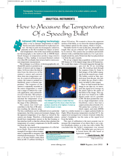
Infrared (IR) imaging technology
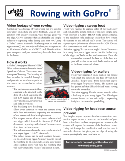
Rowing with GoPro ® Video footage of your rowing Video-rigging a sweep boat
How to Move Canon EF Lenses Yosuke Bando
Mr. Chad Art Foundations Name:_________________________________________
Camera Recommendation for Dental Photography January 2014 Introduction
A Photographer’s E-Guide To Making Sharp Photographs S
IP address of cameras connected to the MI424WR Verizon FiOS Router •
Document 242372
© Copyright 2026
About abcdocz
DMCA / GDPR
Report