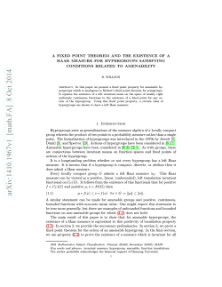
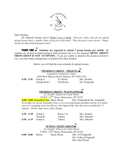
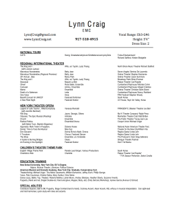
How to Generate Random
Matrices from the Classical
Compact Groups
Francesco Mezzadri
S
ince Random Matrix Theory (RMT) was
introduced by Wishart [17] in 1928, it has
found applications in a variety of areas of
physics, pure and applied mathematics,
probability, statistics, and engineering.
A few examples—far from being exhaustive—
include: analytic number theory, combinatorics,
graph theory, multivariate statistics, nuclear
physics, quantum chaos, quantum information,
statistical mechanics, structural dynamics, and
wireless telecommunications. The reasons for the
ever growing success of RMT are mainly two.
Firstly, in the limit of large matrix dimension the
statistical correlations of the spectra of a family,
or ensemble, of matrices are independent of the
probability distribution that defines the ensemble,
but depend only on the invariant properties of
such a distribution. As a consequence random
matrices turn out to be very accurate models for a
large number of mathematical and physical problems. Secondly, RMT techniques allow analytical
computations to an extent that is often impossible
to achieve in the contexts that they are modelling.
This predictive ability of RMT is particularly
powerful whenever in the original problem there
are no natural parameters to average over.
Although the advantage of using RMT lies in
the possibility of computing explicit mathematical
and physical quantities analytically, it is sometimes necessary to resort to numerical simulations.
The purpose of this article is twofold. Firstly, we
provide the reader with a simple method for generating random matrices from the classical compact
groups that most mathematicians—not necessarily familiar with computer programming —should
Francesco Mezzadri is a Lecturer in Applied Mathematics at the University of Bristol, United Kingdom. His email
address is [email protected].
592
be able to implement in a code of only a few lines.
This is achieved in the section “A Correct and Efficient Algorithm”. Secondly, we discuss in detail
the main ideas, which turn out be fairly general
and quite interesting, behind this algorithm.
An N × N unitary matrix U = (ujk ) is defined
by the relation U ∗ U = UU ∗ = I, which in terms of
the matrix elements reads
(1)
N
X
∗
ujk
ukl =
k=1
N
X
ukj ukl = δjl
and
k=1
N
X
k=1
∗
ujk ukl
=
N
X
ujk ulk = δjl ,
k=1
∗
where U ∗ = (ujk
) is the conjugate transpose
∗
of U, i.e., ujk = ukj . In this article we will use
the symbol to denote complex conjugation, in
order to distinguish it from ∗ , which is reserved
for the conjugate transpose of a matrix. The
constraints (1) simply state that the columns
(rows) of a unitary matrix form an orthonormal
basis in CN . The set U(N) of unitary matrices
forms a compact Lie group whose real dimension
is N 2 ; it is then made into a probability space by
assigning as a distribution the unique measure
invariant under group multiplication, known as
Haar measure. Such a probability space is often
referred to as Circular Unitary Ensemble (CUE).
Usually the correct ensemble to model a particular situation depends on the symmetries of
the problem. Ensembles of unitary matrices are
constructed in two steps: we first identify a subset
U ⊂ U(N) by imposing further restrictions on U;
then we assign to U a probability measure with the
appropriate invariant properties. As well as U(N),
we will discuss how to generate random matrices
from the orthogonal O(N) and unitary symplectic USp(2N) groups with probability distributions
Notices of the AMS
Volume 54, Number 5
given by the respective unique invariant measures. We shall also consider the two remaining
Dyson circular ensembles [2], namely the Circular
Orthogonal Ensemble (COE) and Circular Symplectic Ensemble (CSE). Other symmetric spaces appear
in the applications [18], but we will not concern
ourselves with them.
Writing an algorithm to generate random unitary matrices that is both correct and numerically
stable presents some pitfalls. The reason is that
the conditions (1) imply that the matrix elements
are not independent and thus are statistically correlated. The main ideas discussed in this article
are centered around the QR decomposition and go
back to Wedderburn [16], Heiberger [5] (corrected
by Tanner and Thisted [15]), Stewart [14], and Diaconis and Shahshahani [1]. However, the technical
literature may be difficult to access for a reader
without a background in numerical analysis or
statistics, while the implementation of such techniques is elementary. Another method discussed
in the literature involves an explicit representation
of the matrix elements of U in terms of N 2 independent parameters (Euler angles) [19], but it does
not seem to be equally efficient or convenient.
Before discussing how to generate random matrices it is helpful to give a few examples that show
how they appear in the applications.
In quantum mechanics all the information about
an isolated physical system at a given time t0 is
contained in a state vector ψ0 belonging to a
Hilbert space H —in general infinite dimensional.
The time evolution of ψ0 , i.e., its dynamics, is determined by a unitary operator U. In other words,
at a time t > t0 , ψ0 has evolved into
ψ = Uψ0 .
The fact that U is unitary guarantees that kψk =
kψ0 k = 1, which is required by the probabilistic
interpretation of quantum mechanics.
If the dynamics is complicated—as in heavy nuclei or in quantum systems whose classical limits
are characterized by chaotic dynamics—writing
down an explicit expression for U may be hopeless. Therefore, we can attempt to replace U by
a random operator and check if the predictions
that we obtain are consistent with the empirical
observations. It is also reasonable to simplify the
problem even further and replace U by a random
unitary matrix of finite, but large, dimension. Then
the main question is: What are the matrix space
and the probability distribution that best model
our system?
In physics the symmetries of a problem are
often known a priori, even if the details of the
dynamics remain obscure. Now, suppose that our
system is invariant under time reversal but does
May 2007
U = Ut ,
(3)
where U t denotes the transpose of U. Since there
are no other symmetries in the problem, this is
the only constraint that we can impose. Therefore,
the appropriate matrices that model this physical
system should be symmetric. Let us denote by O
the set of unitary symmetric matrices. If U ∈ O it
can be proved (see Meta [9] p. 499) that it admits
the representation
(4)
U = WWt,
W ∈ U(N).
This factorization is not unique. Let O(N) be the
group of real matrices O such that OO t = O t O =
I and set W ′ = W O. By definition we have
(5)
U = W ′ W ′t = W OO t W t = W W t .
This statement is true also in the opposite direction: if W W t = W ′ W ′t there exists an O ∈ O(N)
such that W ′ = W O. Therefore, O is isomorphic to
the left coset space of O(N) in U(N), i.e.,
O ≅ U(N)/O(N).
(6)
Some Examples and Motivations
(2)
not have any other symmetry. From general considerations (see Mehta [9] p. 36) we know that U
is always conjugate by a unitary transformation
to a symmetric matrix. Therefore, we can always
choose U so that
Since a measure space with total mass equal to
one is a probability space, in what follows we shall
use the two terminologies interchangeably. An ensemble of random matrices is defined by a matrix
space and a probability measure on it. We have
found the former; we are left to identify the latter.
Haar measure, which will be discussed in detail in
the section “Haar Measure and Invariance”, provides a natural probability distribution on U(N);
“natural” in the sense that it equally weighs different regions of U(N), thus it behaves like a uniform
distribution. From the factorization (4) the probability distribution on U(N) induces a measure on
O. As a consequence, if W is Haar distributed the
resulting measure on O will be uniform too. In
the section “A Group Theoretical Interpretation”,
we shall see that such a measure is the unique
probability distribution induced by Haar measure
on O. Therefore, it provides a natural choice to
model a time reversal invariant quantum system.
The space O together with this measure is the COE
ensemble.
If a quantum system does not have any symmetry, then there are no restrictions on U(N), and
the natural choice of probability distribution is
Haar measure. This is the CUE ensemble. If the
system is invariant under time reversal and has
a half-integer spin, then the appropriate ensemble is the CSE. The matrix space of the CSE is
the subset S ⊂ U(2N) whose elements admit the
representation
(7)
U = −W JW t J,
Notices of the AMS
W ∈ U(2N),
593
where
(8)
0
J=
−IN
!
IN
.
0
From the factorization (7) the probability distribution on U(2N) induces a measure on S. As
previously, such a measure is fixed by assigning
Haar measure to U(2N).
The set S is isomorphic to a coset space too. The
unitary symplectic group USp(2N) is the subgroup
of U(2N) whose elements obey the relation
(9)
then W ′ W −1 ∈ USp(2N). Therefore,
S ≅ U(2N)/USp(2N).
The probability distribution of the CSE is the
unique invariant measure induced on the coset
space (11) by Haar measure on U(2N).
From equations (4) and (7) all we need to
generate random matrices in the CUE, COE, and
CSE ensembles is an algorithm whose output is
Haar distributed unitary matrices. The rest of
this article will concentrate on generating random matrices from all three classical compact
groups U(N), O(N), and USp(2N) with probability
distributions given by the respective Haar measures. These groups are not only functional to
constructing matrices in the COE and CSE, but are
also important ensembles in their own right. Indeed, the work of Montgomery [11], Odlyzko [12],
Katz and Sarnak [6], Keating and Snaith [7, 8],
and Rubinstein [13] has shown beyond doubt that
the local statistical properties of the Riemann zeta
function and other L-functions can be modelled by
the characteristic polynomials of Haar distributed
random matrices. Over the last few years the predictive power of this approach has brought about
impressive progress in analytic number theory
that could not have been achieved with traditional
techniques. (See [10] for a collection of review
articles on the subject.)
Haar Measure and Invariance
Since the algorithm we shall discuss is essentially
based on the invariant properties of Haar measure,
in this section we introduce the main concepts that
are needed to understand how it works. We nevertheless begin with another ensemble: the Ginibre
ensemble. Besides being a simpler illustration of
the ideas we need, generating a matrix in the Ginibre ensemble is the first step toward producing a
random unitary matrix.
The space of matrices for the Ginibre ensemble
is GL(N, C), the set of all the invertible N × N
594
1 −|zj k |2
e
.
π
By definition the matrix entries are statistically independent, therefore the joint probability density
function (j.p.d.f.) for the matrix elements is
(12)
SJS t = J.
Therefore, the matrix U in equation (7) does not
change if we replace W with W ′ = W S, where
S ∈ USp(2N). Similarly, if W and W ′ are such that
(10)
U = −W JW t J = −W ′ JW ′t J, W , W ′ ∈ U(2N),
(11)
complex matrices Z = (zjk ); the matrix elements
are independent identically distributed (i.i.d.) standard normal complex random variables. In other
words, the probability density function (p.d.f.) of
zjk is
p(zjk ) =
N
1 Y −|zj k |2
e
π N 2 j,k=1


N
X
2
1
zjk 
= N 2 exp −
π
j,k=1
P (Z) =
(13)
1
exp (− Tr Z ∗ Z) .
π N2
Since P (Z) is a probability density, it is normalized to one, i.e.,
Z
P (Z) dZ = 1,
(14)
2
=
QN
CN
where dZ = j,k=1 dxjk dyjk and zjk = xjk + iyjk .
The j.p.d.f. P (Z) contains all the statistical information on the Ginibre ensemble.
2
Since CN×N ≅ CN , we will use the two notations
according to what is more appropriate for the
context. Thus, we can write
(15)
dµG (Z) = P (Z) dZ
and think of dµG as an infinitesimal volume or
2
measure in CN . If f : CN×N -→ CN×N , we say that
dµG is invariant under f if
(16)
dµG f (Z) = dµG (Z).
Lemma 1. The measure of the Ginibre ensemble is
invariant under left and right multiplication of Z
by arbitrary unitary matrices, i.e.,
(17)
dµG (UZ) = dµG (ZV ) = dµG (Z), U, V ∈ U(N).
Proof. First we need to show that P (UZ) = P (Z);
then we must prove that the Jacobian of the map
(18)
Z ֏ UZ
2
(seen as a transformation in CN ) is one. Since by
definition U ∗ U = I, we have
1
P (UZ) = N 2 exp (− Tr Z ∗ U ∗ UZ)
π
(19)
1
= N 2 exp (− Tr Z ∗ Z) = P (Z).
π
Now, the map (18) is isomorphic to
(20)
X = |U ⊕ · {z
· · ⊕ U}.
Ntimes
It follows immediately that X is a N 2 × N 2 unitary matrix, therefore |det X| = 1. The proof of
right invariance is identical.
Notices of the AMS
Volume 54, Number 5
Because the elements of a unitary matrix are
not independent, writing an explicit formula for
the infinitesimal volume element of U(N) is more
complicated than for the Ginibre ensemble. An
N × N unitary matrix contains 2N 2 real numbers
and the constraints (1) form a system of N 2 real equations. Therefore, U(N) is isomorphic to a
2
N 2 -dimensional manifold embedded in R2N . Such
a manifold is compact and has a natural group
structure that comes from matrix multiplication.
Thus, an infinitesimal volume element on U(N)
will have the form
(21)
dµ(U) = m(α1 , . . . , αN 2 )dα1 · · · dαN 2 ,
where α1 , . . . , αN 2 are local coordinates on U(N).
Every compact Lie group has a unique (up to an
arbitrary constant) left and right invariant measure, known as Haar measure. In other words, if
we denote Haar measure on U(N) by dµH (U), we
have
(22)
dµH (V U) = dµH (UW ) = dµH (U), V , W ∈ U(N).
Although an explicit expression for Haar measure
on U(N) in terms of local coordinates can be
˙yczkowski and Kus [19] for
written down (see Z
a formula), we will see that in order to generate
matrices distributed with Haar measure we only
need to know that it is invariant and unique.
Haar measure normalized to one is a natural
choice for a probability measure on a compact
group because, being invariant under group multiplication, any region of U(N) carries the same
weight in a group average. It is the analogue of the
uniform density on a finite interval. In order to
understand this point consider the simplest example: U(1). It is the set {eiθ } of the complex numbers
with modulo one, therefore it has the topology
of the unit circle S1 . Since in this case matrix
multiplication is simply addition mod 2π , U(1) is
isomorphic to the group of translations on S1 . A
probability density function that equally weighs
any part of the unit circle is the constant density
ρ(θ) = 1/(2π ). This is the standard Lebesgue
measure, which is invariant under translations.
Therefore, it is the unique Haar measure on U(1).
Note that it is not possible to define an “unbiased” measure on a non-compact manifold. For
example, we can provide a finite interval with a
constant p.d.f. ρ(x),
R ∞ but not the whole real line R,
since the integral −∞ ρ(x)dx would diverge.
The QR Decomposition and a Numerical
Experiment
By definition the columns of an N × N unitary
matrix are orthonormal vectors in CN . Thus, if we
take an arbitrary complex N × N matrix Z of full
rank and apply Gram-Schmidt orthonormalization
to its columns, the resulting matrix Q is unitary.
May 2007
It turns out that if the entries of Z are i.i.d. standard complex normal random variables, i.e., if Z
belongs to the Ginibre ensemble, then Q is distributed with Haar measure (see Eaton [3], p. 234,
for a proof). Unfortunately, the implementation of
this algorithm is numerically unstable. However,
we may observe that
(23)
Z = QR,
where R is upper-triangular and invertible. In other words, the Gram-Schmidt algorithm realizes
the QR decomposition. This factorization is widely
used in numerical analysis to solve linear least
squares problems and as the first step of a particular eigenvalue algorithm. Indeed, every linear
algebra package has a routine that implements
it. In most cases, however, the algorithm adopted is not the Gram-Schmidt orthonormalization
but uses the Householder reflections, which are
numerically stable.
Because of this simple observation, at first one
might be tempted to produce a matrix in the
Ginibre ensemble and then to use a black box
QR decomposition routine. Writing such a code
is straightforward. For example, if we choose the
SciPy library in Python, we may implement the
following function:
from scipy import *
def wrong_distribution(n):
“““A Random matrix with the wrong
distribution”””
z = (randn(n,n) + 1j*randn(n,n))/
sqrt(2.0)
q,r = linalg.qr(z)
return q
Unfortunately, as Edelman and Rao observed [4],
the output is not distributed with Haar measure.
It is instructive to give an explicit example of this
phenomenon.
A unitary matrix can always be diagonalized in
U(N). Therefore, its eigenvalues {eiθ1 , . . . , eiθN } lie
on the unit circle. A classical calculation in RMT
(see Mehta [9] pp. 203–205) consists of computing
the statistical correlations among the arguments
θj . The simplest correlation function to determine
is the density of the eigenvalues ρ(θ), or—as
sometimes it is called—the one-point correlation.
Since Haar measure is the analogue of a uniform
distribution, each set of eigenvalues must have the
same weight, therefore the normalized eigenvalue
density is
1
.
2π
It is important to point out that equation (24) does
not mean that the eigenvalues are statistically
uncorrelated.
(24)
Notices of the AMS
ρ(θ) =
595
Testing (24) numerically is very simple. We
generated 10, 000 random unitary matrices using wrong_distribution(n). The density of the
eigenvalues of such matrices is clearly not constant
(Figure 1(a)). Figure 1(b) shows the histogram of
the spacing distribution, which deviates from the
theoretical prediction too. This statistic is often
plotted because it encodes the knowledge of all
the spectral correlations and is easy to determine
empirically. For unitary matrices it is defined as
follows. Take the arguments of the eigenvalues
and order them in ascending order:
θ1 ≤ θ2 ≤ . . . ≤ θN .
(25)
The normalized distances, or spacings, between
consecutive eigenvalues are
(a) Eigenvalue density
N
(θj+1 − θj ), j = 1, . . . , N.
2π
The spacing distribution p(s) is the probability
density of s. (For a discussion on the spacing
distribution see Mehta [9] p. 118.)
It is worth emphasizing that the QR decomposition is a standard routine. The most commonly
known mathematical software packages like Matlab, Mathematica, Maple, and SciPy for Python
essentially use a combination of algorithms found
in LAPACK routines. Changing software would not
alter the outcome of this numerical experiment.
(26)
sj =
A Correct and Efficient Algorithm
What is wrong with standard QR factorization
routines? Where do they differ from the GramSchmidt orthonormalization? Why is the probability distribution of the output matrix not Haar
measure?
The main problem is that QR decomposition is
not unique. Indeed, let Z ∈ GL(N, C) and suppose
that Z = QR, where Q is unitary and R is invertible
and upper-triangular. If
(27)
 iθ

e 1


..
 = diag eiθ1 , . . . , eiθN ,
Λ=
.


eiθN
then
(28)
′
Q = QΛ
and
′
−1
R =Λ R
are still unitary and upper-triangular, respectively.
Furthermore,
(29)
Z = QR = Q′ R ′ .
Therefore, the QR decomposition defines a multivalued map
(30)
QR : GL(N, C) -→ U(N) × T(N),
where T(N) denotes the group of invertible uppertriangular matrices.
In order to make the mapping (30) single-valued,
we need to specify the algorithm that achieves the
factorization. In most applications such a choice
596
(b) Spacing distribution
Figure 1. Empirical histograms of the density
of the eigenvalues and of the spacing
distributions compared with the theoretical
curves for the CUE. The data are computed
from the eigenvalues of ten thousand 50 x 50
random unitary matrices obtained from the
routine wrong_distribution(n).
is dictated only by the performance and stability of the code. For our purposes, however, the
subset of U(N) × T(N), in which the output of
the QR decomposition is chosen, is fundamental
and we need to pay particular attention to it. It is
convenient from a mathematical point of view to
introduce a variation of the mapping (30), which
is not only single-valued but also one-to-one. In
this way we will not have to refer all the time
to a specific algorithm. Indeed, the idea is that
we should be able to alter the output of a QR
decomposition routine without even knowing the
algorithm implemented.
We first need
Notices of the AMS
Volume 54, Number 5
Lemma 2. Equation (29) implies (28), where Λ ∈
Λ(N) and Λ(N) denotes the group of all unitary
diagonal matrices (27).
Theorem 1. Suppose that the map (32) satisfies
the hypothesis (33). Then it decomposes the measure (15) of the Ginibre ensemble as
Proof. Equation (29) can be rearranged as
(36)
Q−1 Q′ = RR ′−1 .
(31)
Proof. We have
Since U(N) and T(N) are groups, both sides of
equation (31) must belong to U(N) ∩ T(N). By
definition the inverse of a unitary matrix U is its
conjugate transpose and the inverse of an uppertriangular matrix is upper-triangular. Therefore,
if a matrix is both unitary and upper-triangular it
must be diagonal, i.e., Λ(N) = U(N) ∩ T(N).
This lemma suggests that, more naturally, instead of the QR factorization (30) we should
consider a one-to-one map
(32)
QR : GL(N, C) -→ U(N) × Γ (N),
where Γ (N) = T(N)/Λ(N) is the right coset space
of Λ(N) in T(N). We construct (32) as follows: we
first define it on a class of representatives of Γ (N)
using the QR factorization; then we extend it to the
whole Γ (N). However, since the QR decomposition
is not unique, there is a certain degree of arbitrariness in this definition. We need to find a map
under which the measure of the Ginibre ensemble
induces Haar measure on U(N). The main tool to
achieve this goal is the invariance under group
multiplication of Haar measure and its uniqueness. Thus, our choice of the decomposition (32)
must be such that if
(33)
Z ֏ (Q, γ) then UZ ֏ (UQ, γ)
dµG (UZ) = dµG (Z)
for any U ∈ U(N). As a consequence, if the
map (32) satisfies (33) the induced measure on
U(N) will be invariant under left multiplication
too and therefore must be Haar measure.
How do we construct the map (32)? A class of
representatives of Γ (N) can be chosen by fixing the
arguments of the elements of the main diagonal
of R ∈ T(N). Let us impose that such elements
all be real and strictly positive. Using (28) we can
uniquely factorize any Z ∈ GL(N, C) so that the
main diagonal of R has this property. It follows
that if Z = QR, then
(35)
UZ = UQR,
U ∈ U(N).
This QR decomposition of UZ is unique within the
chosen class of representatives of Γ (N). Therefore,
the resulting map (32) obeys (33). Finally, we arrive
at
May 2007
(37a)
dµG (U Z) = dµG (Z)
by lemma 1
(37b)
= dµ(U Q, γ) = dµ(Q, γ)
(37c)
= dµH (Q) × dµΓ (N) (γ)
by equation (33)
by the uniqueness
of Haar measure.
The choice of the class of representatives that
we made coincides exactly with outcome of the
Gram-Schmidt orthonormalization. The output of
standard QR decomposition routines are such that
if Z ֏ (Q, R) then UZ ֏ (Q′ , R ′ ) with Q′ ≠ UQ
and R ′ ≠ R. Therefore, the corresponding map (32)
does not obey (33) and theorem 1 does not hold.
We can now give a recipe to create a random
unitary matrix with distribution given by Haar
measure.
(38)
with the same γ ∈ Γ (N) and for any U ∈ U(N).
This property implies that left multiplication of Z
by a unitary matrix reduces, after the decomposition, to the left action of U(N) into itself. But
lemma 1 states that
(34)
dµG (Z) = dµH (Q) × dµΓ (N) (γ).
(1) Take an N ×N complex matrix Z whose entries are complex standard normal random
variables.
(2) Feed Z into any QR decomposition routine.
Let (Q, R), where Z = QR, be the output.
(3) Create the following diagonal matrix

 r11

Λ=

|r11 |
..
.
rNN
|rNN |

,

where the rjj s are the diagonal elements
of R.
(4) The diagonal elements of R ′ = Λ−1 R are
always real and strictly positive, therefore
the matrix Q′ = QΛ is distributed with
Haar measure.
The corresponding Python function is:
from scipy import *
def haar_measure(n):
“““A Random matrix distributed with
Haar measure”””
z = (randn(n,n) + 1j*randn(n,n))/
sqrt(2.0)
q,r = linalg.qr(z)
d = diagonal(r)
ph = d/absolute(d)
q = multiply(q,ph,q)
return q
If we repeat the numerical experiment discussed
in the section “The QR Decomposition and a Numerical Experiment”, using this routine, we obtain
the histograms in Figure 2, which are consistent
with the theoretical predictions.
Notices of the AMS
597
where 1 is the identity and i1 , i2 , i3 are the
quaternion units; they obey the algebra
(40)
i12 = i22 = i32 = i1 i2 i3 = −1.
We can also define the conjugate of q,
(41)
q = a · 1 − bi1 − ci2 − di3 ,
as well the norm
(42)
(a) Eigenvalue density
2
kqk = q q = q q = a2 + b2 + c 2 + d 2 .
When c = d = 0, H reduces to C and q is simply
the complex conjugate of q.
In analogy with RN and CN —provided we are
careful with the fact that multiplication in H is
not commutative—we can study the space HN .
Elements in HN are N-tuples q = (q1 , . . . , qN ). The
bilinear map
(43)
hp, qi =
N
X
pj qj ,
p, q ∈ HN ,
j=1
is the analogue of the usual Hermitian inner product in CN , and the norm of a quaternion vector is
simply
(44)
2
kqk = hq, qi =
N
X
2
qj .
j=1
(b) Spacing distribution
Figure 2. Empirical histograms of the density
of the eigenvalues and of the spacing
distributions compared with the theoretical
curves for the CUE. The data are computed
from the eigenvalues of ten thousand 50x 50
random unitary matrices output of the
function haar_measure(n).
The Unitary Symplectic Group USp(2N)
Up to now we have only considered U(N). The discussion for O(N) is identical, except that the input
matrix of the QR decomposition routine must be
real. Unfortunately, however, for USp(2N) there
are no black box routines that we can use, and we
must put more effort into writing an algorithm.
The algebra of unitary symplectic matrices
can be rephrased in terms of Hamilton’s quaternions; it is convenient for our purposes to use
this formalism. A quaternion q ∈ H is a linear
combination
(39)
598
q = a · 1 + bi1 + ci2 + di3 ,
a, b, c, d ∈ R,
Similarly, GL(N, H) is the group of all the N × N
invertible matrices with quaternion elements.
The quaternion units admit a representation in
terms of the 2 × 2 matrices
(45a)
!
!
!
0
1
i
0
1 0
, e2 =
, e1 =
I2 =
−1 0
0 −i
0 1
!
0 i
,
and e3 =
i 0
where
(45b) 1 ֏ I2 ,
i1 ֏ e1 ,
i2 ֏ e2
and i3 ֏ e3 .
Thus, q = a · 1 + bi1 + ci2 + di3 is mapped into the
complex matrix
!
z
w
(46a)
A=
−w z
where z = a + ib and w = c + id. In addition
!
z −w
∗
(46b)
q֏A =
.
w
z
Equations (46) generalize to an arbitrary N × N
quaternion matrix Q, which can be represented in
terms of a 2N × 2N complex matrix Q using the
decomposition
(47) Q ֏ Q = Q0 ⊗ I2 + Q1 ⊗ e1 + Q2 ⊗ e2 + Q3 ⊗ e3 ,
where Q0 , Q1 , Q2 , and Q3 are arbitrary N × N
real matrices. Proceeding in the same fashion, if
Q ∈ GL(N, H) we define its conjugate transpose
∗
∗
Q∗ = (qjk
) by setting qjk
= q kj .
The symplectic group Sp(N) is the subset of
GL(N, H) whose matrices satisfy the identity S∗ S =
Notices of the AMS
Volume 54, Number 5
SS∗ = I. Because of the analogy between U(N) and
Sp(N), the latter is sometimes called the hyperunitary group and is denoted by U(N, H). The
usefulness of the quaternion algebra lies in
Theorem 2. The groups Sp(N) and USp(2N) are
isomorphic, i.e.
(48)
USp(2N) ≅ Sp(N).
Proof. It is convenient to replace the skewsymmetric matrix J in the definition (9) with


0
1


..


.

−1 0




..
..
..
 = I ⊗ e2 .
(49)
Ω=
.
.
.




..


.

0
1
−1 0
This substitution is equivalent to a permutation
of the rows and columns of J, therefore it is simply a conjugation by a unitary matrix.
We first prove that if S ∈ Sp(N), then its complex representation S belongs to USp(2N). By
equation (47) S∗ is mapped to
(50) S0t ⊗ I2 − S1t ⊗ e1 − S2t ⊗ e2 − S3t ⊗ e3 = −Ω S t Ω,
which follows from the identities
(51)
(A⊗B)t = At ⊗B t and (A⊗B)(C ⊗D) = AC ⊗BD,
The important fact that we need to pay attention
to is that
Q∗ ֏ Q ∗ ,
(54)
if and only if the coefficients of the quaternion
units are real numbers. This is a straightforward
consequence of the representation (46a).
Let S ∈ USp(2N) be the complex representation of the quaternion matrix S, but assume that
S∗ is not mapped into S ∗ . It is still true, however,
that
S∗ ֏ −Ω S t Ω,
(55)
because equation (50) is only a consequence of
matrix manipulations. But since S is unitary symplectic S ∗ = −Ω S t Ω, which is a contradiction.
The algebra of Sp(N) is the generalization to
Hamilton’s quaternions of the algebra of U(N).
Therefore, it is not surprising that the discussion
in the section “A Correct and Efficient Algorithm”
is not affected by replacing GL(N, C) and U(N)
with GL(N, H) and Sp(N) respectively. Thus, since
Sp(N) and USp(2N) are isomorphic, USp(2N) and
Sp(N) have the same Haar measure dµH . In particular, we can introduce the quaternion Ginibre
ensemble, which is the set GL(N, H) equipped with
the probability density
P (Z) =
(56)
and from the algebra (40) of the quaternion units.
As a consequence,
(52)
SS∗ ֏ −S Ω S t Ω = I.
Therefore, the matrix S is symplectic. Combining
equations (46b) and (50) gives
(53)
− Ω St Ω = S∗,
j,k=1
Quaternion matrices can be factorized by the
QR decomposition too: for any Z ∈ GL(N, H) we
can always write
Z = QR,
(57)
thus S ∈ USp(2N).
We now need to show that if S ∈ USp(2N) then
it is the representation of a matrix S ∈ Sp(N).
This statement follows if we prove that S admits
a decomposition of the form (47), where S0 , S1 , S2 ,
and S3 must be real N × N matrices. If this is true,
then the argument of the first part of the proof
can simply be reversed.
Let us allow the coefficients a, b, c, and d in
the definition (39) to be complex numbers. The
definitions of conjugate quaternion (41) and conjugate transpose of a quaternion matrix, however,
remain the same. The matrices (45a) form a basis in C2×2 . Therefore, any 2 × 2 complex matrix
can be represented as a linear combination of I2 ,
e1 , e2 , and e3 . Thus, any matrix Q ∈ C2N×2N admits a decomposition of the form (47), but now
the matrices Q0 , Q1 , Q2 , and Q3 are allowed to be
complex. In other words, Q is always the representation of a quaternion matrix Q, but in general the quaternion units have complex coefficients.
May 2007
1
π 2N 2
1
∗
2 exp (− Tr Z Z) =
π 2N

N
X
2
zjk  .
exp −
where Q ∈ Sp(N) and R is an invertible and
upper-triangular quaternion matrix. Now, let
(58)
n
Λ(N, H) = Λ ∈ T(N, H) Λ = diag (q1 , . . . , qN ) ,
o
qj = 1, j = 1, . . . , N ,
where T(N, H) is the group of invertible uppertriangular quaternion matrices. Furthermore, let
Γ (N, H) = T(N, H)/Λ(N, H) be the right coset
space of Λ(N, H) in T(N, H). We have the following
Theorem 3. There exists a one-to-one map
QR : GL(N, H) -→ Sp(N) × Γ (N, H)
(59)
such that
(60)
Z ֏ (Q, γ) and
UZ ֏ (UQ, γ),
where γ = Λ(N, H)R. Furthermore, it factorizes
the measure dµG of the Ginibre ensemble as
(61)
dµG (Z) = dµH (Q) × dµΓ (N,H) (γ).
Notices of the AMS
599
We leave proving these generalizations as an
exercise for the reader.
Householder Reflections
Theorem 3 provides us with the theoretical tools
to generate a random matrix in USp(2N). However, when we implement these results in computer
code, we need to devise an algorithm whose output satisfies the condition (60). The first one that
comes to one’s mind is Gram-Schmidt orthonormalization. But given that black box routines for
quaternion matrices do not exist on the market
and that we are forced to write the complete code
ourselves, we may as well choose one that is numerically stable and that as it turns out, requires
the same effort. The most common algorithm that
achieves the QR decomposition uses the Householder reflections. For the sake of clarity, we will
discuss this method for O(N); the generalizations
to U(N) and Sp(N) are straightforward.
Given an arbitrary vector v ∈ Rm , the main idea
of the Householder reflections is to construct a
simple orthogonal transformation Hm (dependent
on v) such that
(62)
Hm v = kvk e1 ,
where e1 = (1, 0, . . . , 0) ∈ Rm . For any real matrix
X = (xjk ), HN is determined by replacing v in
equation (62) with the first column of X. The
product HN X will have the structure


r11 ∗ · · · ∗
 0 ∗ · · · ∗


(63)
HN X = 
..
.. 
 ..
,
 .
.
.
0 ∗ ··· ∗
where
(64)
r11 = kvk =
Then, define the matrix

1


e N−1 = 
(65)
H
 0
qP
N
j=1
x2j1 .

0


,

HN−1
where
(66)
HN−1 (v′ )v′ = kv′ k e1 .
In this case v′ is the (N − 1)-dimensional vector
obtained by dropping the first element of the second column of the matrix (63). We proceed in this
fashion until the matrix
(67)
e1H
e2 · · · H
e N−1 HN X
R=H
is upper-triangular with diagonal entries r11 , . . . , rNN .
The product
(68)
600
t
e N−1
e 2t H
e 1t
Q = HNt H
···H
Figure 3. Householder reflection in R2 .
is by construction an orthogonal matrix. In equae m denotes the block matrix
tions (67) and (68) H
!
e m = IN−m
(69)
H
,
Hm
where Hm is defined in equation (62).
The matrix Hm is constructed using elementary
geometry. Consider a vector in the plane, v =
(x1 , x2 ), and assume, for simplicity, that x1 > 0.
ˆ denote the unit vector along
Furthermore, let u
the interior bisector of the angle φ that v makes
with the x1 -axis, i.e.,
(70)
v + kvk e1
ˆ= u
v + kvk e1 ,
where e1 is the unit vector along the x1 -axis.
ˆ is
The reflection of v along the direction of u
kvk e1 (see Figure 3). Reflections are distancepreserving linear transformations, therefore their
representations in an orthonormal basis are orthogonal matrices. In this simple example it can
be constructed from elementary linear algebra:
(71)
ˆt .
H2 (v) = −I + 2ˆ
uu
Finally, we obtain
(72)
H2 (v)v = kvk e1 .
It is worth noting that H2 depends only on the
direction of v and not on its modulus. Thus we
can rewrite equation (72) as
(73)
H2 (ˆ
v)ˆ
v = e1 ,
ˆ = v/ kvk.
where v
The generalization to arbitrary dimensions is
straightforward. For any vector v ∈ Rm , the Householder reflection is defined as
ˆt ,
(74)
Hm (ˆ
v) = ∓ I − 2ˆ
uu
where
(75)
Notices of the AMS
v ± kvk e1
ˆ= u
v ± kvk e1 .
Volume 54, Number 5
definitions of the Householder reflections. A suitable choice for U(N) is
Furthermore, we have
(76)
Hm (ˆ
v)ˆ
v = e1 .
How do we choose the sign in the right-hand
side of equation (75)? From a mathematical point
of view such a choice is irrelevant: in both cases
Hm (ˆ
v) maps v into a vector whose only component different from zero is the first one. However,
numerically it can be important. The square of the
denominator in (75) is
v ± kvk e1 2 = 2 kvk (kvk ± x1 ) ,
(77)
where x1 is the first component of v. If x1 is comparable in magnitude to kvk and negative (positive)
and we choose the plus (minus) sign, then the term
(78)
kvk ± x1 ,
could be very small and cancellations with significant round-off errors may occur. Therefore, the
Householder transformation to be implemented
in computer code should be
ˆt ,
(79)
Hm (ˆ
v) = − sgn(x1 ) I − 2ˆ
uu
(83)
ˆ∗ ) .
Hm (ˆ
v) = −e−iθ (I − 2ˆ
uu
ˆ is
The unit vector u
ˆ=
u
(84)
where v = (x1 , . . . , xm ) ∈ Cm and x1 = eiθ |x1 |. The
matrix Hm (ˆ
v) is unitary and
Hm (ˆ
v)ˆ
v = e1 .
(85)
Note that the introduction of eiθ in equations (83)
and (84) takes into account both the potential cancellations and the correct values of the arguments
of the diagonal elements of the upper-triangular
matrix R: equation (85) implies that all the rjj s are
real and strictly positive.
For Sp(N) we have
(86)
ˆ∗ ) ,
Hm (ˆ
v) = −q (I − 2ˆ
uu
with
(87)
where
(80)
′
ˆt ,
Hm
(ˆ
v) = I − 2ˆ
uu
ˆ as in (75). Therefore,
with the same u
(82)
′
Hm
(ˆ
v)ˆ
v = ∓e1 .
As a consequence, the signs of the diagonal elements of R are random. This is the reason why the
output of black box QR decomposition routines
must be modified in order to obtain orthogonal
matrices with the correct distribution.
Besides being numerically stable, this algorithm
has another advantage with respect to GramSchmidt orthonormalization. In most applications
of numerical analysis Q need not be computed
explicitly, only Qw does, where w is a specific
vector. Generating all the Householder reflections
is an O(N 2 ) process and computing HN w requires
O(N) operations—it just evaluates the scalar product (ˆ
u, w). Successively multiplying HN , . . . , H1 into
w is an O(N 2 ) process. Therefore, it takes in total
O(N 2 ) operations to compute Qw. Instead, GramSchmidt orthonormalization is an O(N 3 ) process.
However, if Q is explicitly needed, computing the
product (68) requires O(N 3 ) operations too.
The generalizations to U(N) and Sp(N) are
straightforward. The only differences are in the
May 2007
ˆ=
u
ˆ + qe1
v
,
kˆ
v + qe1 k
where v = (x1 , . . . , xm ) ∈ Hm and x1 = q kx1 k. Also
in this case
ˆ + sgn(x1 )e1
v
.
ˆ= u
v
ˆ + sgn(x1 )e1 The additional factor of sgn(x1 ) in the righthand side of equation (79) assures that there
is no ambiguity in the sign of the right-hand
side of equation (76). In turn, it guarantees that
all the diagonal elements of the upper-triangular
matrix R are positive. This is not the definition
of Householder reflection used in standard QR
decomposition routines. Usually,
(81)
ˆ + eiθ e1
v
,
kˆ
v + eiθ e1 k
(88)
Hm (ˆ
v)ˆ
v = e1 .
A Group Theoretical Interpretation
We now know how to generate random matrices
from any of the classical compact groups U(N),
O(N), and Sp(N). In order to achieve this goal, we
have used little more than linear algebra. However
simple and convenient this approach is (after all
linear algebra plays a major role in writing most
numerical algorithms), it hides a natural group
theoretical structure behind the Householder reflections, which was uncovered by Diaconis and
Shahshahani [1]. Indeed, generating a random matrix as a product of Householder reflections is only
one example of a more general method that can
be applied to any finite or compact Lie group. Our
purpose in this section is to give a flavor of this
perspective. For the sake of clarity, as before, we
will discuss the orthogonal group O(N); the treatment of U(N) and Sp(N) is, once again, almost
identical.
The need for a more general and elegant approach arises also if one observes that there is
one feature of the QR decomposition that may
not be entirely satisfactory to a pure mathematician: Why in order to generate a random point
on an N(N − 1)/2-dimensional manifold—O(N)
in this case—do we need to generate N 2 random
numbers? It does not look like the most efficient
option, even if it is a luxury that can be easily
afforded on today’s computers.
We will first show how the key ideas that we
want to describe apply to finite groups, as in this
setting they are more transparent. Suppose that
Notices of the AMS
601
we need to generate a random element g in a finite
group ΓN . In this context, if ΓN has p elements,
uniform distribution simply means that the probability of extracting any g ∈ ΓN is 1/p. In addition,
we assume that there exists a chain of subgroups
of ΓN :
(89)
Γ1 ⊂ Γ2 ⊂ · · · ⊂ ΓN .
In practical situations it is often easier to generate
˜ in a smaller subgroup, say
a random element g
Γm−1 ∈ ΓN , than in ΓN itself; we may also know
how to take a random representative gm in the left
coset Cm = Γm /Γm−1 . Now, write the decomposition
(90)
Γm ≅ Cm × Γm−1 .
Once we have chosen a set of representatives of
Cm , an element g ∈ Γm is uniquely factorized as
˜, where gm ∈ Cm . If both gm and g
˜ are
g = gm g
uniformly distributed in Cm and Γm−1 respectively,
then g is uniformly distributed in Γm .
We can apply this algorithm iteratively starting from Γ1 and eventually generate a random
element in ΓN . In other words, we are given the
decomposition
(91)
ΓN ≅ CN × · · · × C2 × Γ1 .
An element g ∈ ΓN has a unique representation as
a product
(92)
g = gN · · · g1 ,
where gm is a representative in Cm . If the gm s are
uniformly distributed in Cm so is g in ΓN . This is
known as the subgroup algorithm [1].
This technique applies to random permutations
of N letters. The chains of subgroups is
(93)
{Id} ⊂ S2 ⊂ · · · ⊂ SN ,
where Sm is the m-th symmetric group. Other
examples include generating random positions of
Rubik’s cube and random elements in GL(N, Fp ),
where Fp is a finite field with p elements.
For O(N) the decompositions (91) and (92)
are hidden behind the factorization (68) in terms
of Householder reflections. Indeed, the subgroup
algorithm for O(N) is contained in
Proof. Suppose we construct O ∈ O(N) distributed with Haar measure by factorizing a matrix X in
the Ginibre ensemble as described in the section
“Householder Reflections”. The random matrix O
is the product of Householder reflections (68) and
each factor Hm (ˆ
vm ) is a function of the unit vecˆm ∈ Sm−1 only. We need to show that such
tor v
ˆm s are independent and uniformly distributed in
v
Sm−1 for m = 1, . . . , N.
At each step in the construction of the uppertriangular matrix (67), the matrix multiplied by
the m-th Householder reflection, i.e.,
(96)
Xm = Hm (ˆ
vm ) · · · HN−1 (ˆ
vN−1 )HN (ˆ
vN )X,
is still in the Ginibre ensemble. All its elements
are, therefore, i.i.d. normal random variables. This
is a consequence of the invariance
(97)
dµG (OX) = dµG (X),
of the measure of the Ginibre ensemble. Now,
ˆm = (x1 , . . . , xm ) is constructed by taking the
v
m-th dimensional vector vm obtained by dropping the first N −m elements of the (N −m +1)-th
column of Xm . The components of vm are i.i.d.
normal random variables. It follows that the p.d.f.
of vm is
m
1 Y
P (vm ) = m/2
(98)
exp −x2j
π
j=1


m
X
1
1
x2j  = m/2 exp − kvm k2 .
= m/2 exp −
π
π
j=1
Since P (vm ) depends only on the length of vm ,
and not on any angular variable, the unit vector
ˆm = vm / kvm k is uniformly distributed in Sm−1
v
ˆk for k ≠ m.
and is statistically independent of v
Theorem 4 is more transparent than relying on
the QR decomposition, which seems only a clever
technical trick. If nothing else, the counting of
the number of degrees of freedom matches. In
fact, the dimension of the unit sphere Sm−1 is
m − 1. Thus, the total number of independent real
parameters is
(99)
N
X
(m − 1) =
m=1
ˆ1 , . . . , v
ˆN be uniformly distributTheorem 4. Let v
ed on S0 , . . . , SN−1 respectively, where
(94)
n
o
Pm
ˆm = (x1 , . . . , xm ) ∈ Rm j=1 x2j = 1
Sm−1 = v
is the unit sphere in Rm . Furthermore, let Hm (ˆ
v) be
the m-th Householder reflection defined in equation (79). The product
(95)
O = HN (ˆ
vN )HN−1 (ˆ
vN−1 ) · · · H2 (ˆ
v2 )H1 (ˆ
v1 )
is a random orthogonal matrix with distribution
given by Haar measure on O(N).
602
O ∈ O(N),
N(N − 1)
.
2
Why is theorem 4 the subgroup algorithm for
O(N)? As we shall see in theorem 5, the factorization (95) is unique—provided that we restrict to
the definition (79) of the Householder reflections.
This means that
(100)
O(N) ≅ SN−1 × · · · × S1 × O(1),
where
(101)
O(1) ≅ S0 = {−1, 1}.
If we proceed by induction, we obtain
(102)
Notices of the AMS
O(N) = SN−1 × O(N − 1).
Volume 54, Number 5
Therefore, a matrix O ∈ O(N) admits a unique
representation as
(103)
where
(104)
(112)
O = HN (ˆ
vN )Ω,
1


Ω=
 0
0
e
O





Theorem 5. The left coset space of O(N − 1) in
O(N) is isomorphic to SN−1 , i.e.,
where
ˆ + sgn(x1 )e1
v
ˆ= u
v
ˆ + sgn(x1 )e1 ˆ.
and x1 is the first component of v
Proof. The group of N × N matrices Ω defined in
equation (104) is isomorphic to O(N − 1). Since
(108)
Ωe1 = e1 ,
O(N − 1) can be identified with the subgroup of
O(N) that leave e1 invariant, i.e.,
(109)
O(N − 1) = O ∈ O(N) Oe1 = e1 .
Now, if two matrices O and O ′ belong to the same
coset, then
(110)
ˆ
Oe1 = O ′ e1 = v
and vice versa. In other words, cosets are specified by where e1 is mapped. Furthermore, since
kOe1 k = 1, we see that they can be identified
with the points in the unit sphere. Finally, the
map (106) is one-to-one and is such that
(111)
ˆ.
HN (ˆ
v)e1 = v
Therefore, HN spans a complete class of representatives.
Incidentally, theorem 4 implies
1
The Householder reflections defined in equation (79) are
not continuous at e1 . Indeed, it can be proved that there
is no continuous choice of coset representatives. In the
section “Householder Reflections”, this distinction was superfluous: if v is randomly generated, the probability that
v = αe1 is zero.
May 2007
What is the meaning of dµSN−1 ? Given that we
are dealing with uniform random variables, it is
quite natural that we end up with the uniform
measure. In this case, however, it has a precise
group theoretical interpretation. Left multiplication of the right-hand side of equation (103) by
O ′ ∈ O(N) induces a map on the coset space:
(113)
O ′ HN (ˆ
v)Ω = HN (ˆ
v′ )Ω′ Ω = HN (ˆ
v′ )Ω′′ .
Since the decomposition (103) is unique the transˆ֏v
ˆ′ is well defined. This map can be
formation v
easily determined. A coset is specified by where
e1 is mapped, therefore
(114)
O(N)/O(N − 1) ≅ SN−1 .
A complete class of representatives is provided by
the map 1 HN : SN−1 -→ O(N),
(
ˆt ) if v
ˆ ≠ e1 ,
− sgn(x1 ) (I − 2ˆ
uu
(106) HN (ˆ
v) =
ˆ = e1 ,
IN
if v
(107)
dµO(N) = dµSN−1 × dµO(N−1),
where dµSN−1 is the uniform measure on SN−1 .

e ∈ O(N − 1). A consequence of theorem 4
and O
ˆN is uniformly distributed in SN−1 and
is that if v
e is distributed with Haar measure on O(N − 1),
O
then O is Haar distributed too. The final link with
the subgroup algorithm is given by
(105)
Corollary 1. Let dµO(N) and dµO(N−1) be the Haar
measures on O(N) and O(N −1) respectively. Then
ˆ=v
ˆ′ = HN (ˆ
O ′ HN (ˆ
v)e1 = O ′ v
v′ )e1 .
ˆ is uniformly distributed on the unit circle so is
If v
ˆ′ = Oˆ
v
v. Thus, dµSN−1 is the unique measure on the
coset space O(N)/O(N −1) invariant under the left
action of O(N). Its uniqueness follows from that
of Haar measure and from the factorization (112).
Corollary 1 is a particular case of a theorem
that holds under general hypotheses for topological compact groups. Indeed, let Γ be such a group,
Ξ a closed subgroup and C = Γ /Ξ. Furthermore,
let dµΓ , dµC and dµX be the respective invariant
measures, then
(115)
dµΓ = dµΞ × dµC .
Acknowledgements
This article stems from a lecture that I gave at the
summer school on Number Theory and Random
Matrix Theory held at the University of Rochester
in June 2006. I would like to the thank the organizers David Farmer, Steve Gonek, and Chris Hughes
for inviting me. I am also particularly grateful to
Brian Conrey, David Farmer, and Chris Hughes for
the encouragement to write up the content of this
lecture.
References
[1] P. Diaconis and M. Shahshahani, The subgroup algorithm for generating uniform random
variables, Prob. Eng. Inf. Sc. 1 (1987), 15–32.
[2] F. M. Dyson, The threefold way. Algebraic structure
of symmetry groups and ensembles in quantum
mechanics, J. Math. Phys. 3 (1962), 1199–1215.
[3] M. L. Eaton, Multivariate Statistics: A Vector Space
Approach, Wiley and Sons, New York, NY, 1983.
[4] A. Edelman and N. R. Rao, Random matrix theory,
Acta Num. 14 (2005), 233–297.
[5] R. M. Heiberger, Algorithm AS127. Generation of
random orthogonal matrices, App. Stat. 27 (1978),
199–206.
Notices of the AMS
603
[6] N. M. Katz and P. Sarnak, Random matrices, Frobenius eigenvalues, and monodromy, Amer. Math.
Soc. Colloquium Publications, 45, Amer. Math. Soc.,
Providence, RI, 1999.
[7] J. P. Keating and N. C. Snaith, Random matrix
theory and ζ(1/2 + it), Commun. Math. Phys. 214
(2000), 57–89.
[8]
, Random matrix theory and L-functions at
s = 1/2, Commun. Math. Phys. 214 (2000), 91–110.
[9] M. L. Mehta, Random matrices, Elsevier, San Diego,
CA, 2004.
[10] Recent perspectives in random matrix theory and
number theory, LMS Lecture Note Series, 322,
(F. Mezzadri and N. C. Snaith, eds.), Cambridge
University Press, Cambridge, 2005.
[11] H. L. Montgomery, The pair correlation of zeros of
the zeta function, Analytic Number Theory: Proc.
Symp. Pure Math. (St. Louis, MO, 1972), vol. 24,
Amer. Math. Soc., Providence, RI, 1973, pp. 181–93.
[12] A. M. Odlyzko, The 1020 -th zero of the Riemann
zeta function and 70 million of its neighbors,
1989,
http://www.dtc.umn.edu/∼odlyzko/
unpublished/index.html.
[13] M. Rubinstein, Low-lying zeros of L-functions and
random matrix theory, Duke Math. J. 109 (2001),
147–181.
[14] G. W. Stewart, The efficient generation of random
orthogonal matrices with an application to condition estimators, SIAM J. Num. Anal. 17 (1980),
403–409.
[15] M. A. Tanner and R A. Thisted, A remark on
AS127. Generation of random orthogonal matrices,
App. Stat. 31 (1982), 190–192.
[16] R. W. M. Wedderburn, Generating random rotations, Research report, Rothamsted Experimental
Station (1975).
[17] J. Wishart, The generalised product moment distribution in samples from a normal multivariate
population, Biometrika 20A (1928), 32–52.
[18] M. R. Zirnbauer, Riemannian symmetric superspaces and their origin in random-matrix theory,
J. Math. Phys. 37 (1996), 4986–5018.
˙yczkowski and M. Kus, Random unitary
[19] K. Z
matrices, J. Phys. A: Math. Gen. 27 (1994),
4235–4245.
604
Notices of the AMS
Volume 54, Number 5