
How to Measure Heat Capacity at Low Temperatures Chapter 2
Chapter 2
How to Measure Heat Capacity at Low
Temperatures
Abstract This chapter is devoted to the description of calorimetric techniques
used to measure heat capacity of solids: pulse heat calorimetry (Sect. 2.3),
relaxation calorimetry (Sect. 2.4), dual slope calorimetry (Sect. 2.5), a.c. calorimetry (Sect. 2.6), differential scanning calorimetry (Sect. 2.7). Examples of
measurements of heat capacity are reported in Sects. 2.3 and 2.4.
2.1 Introduction
Specific heat defined by (1.4) is useful only if the material is homogeneous. In this
chapter, the heat capacity of the sample under measurement will always be considered in order to also include data about inhomogeneous devices of cryogenic
interest (see, e.g., Ref. [1]).
When a power, P(t), is supplied to an isothermal sample of heat capacity
CS(T) in adiabatic conditions, the sample heating is described by
PðtÞdt ¼ CS ðTÞdT:
ð2:1Þ
If the initial temperature (at t = t0) of the sample is T0, at the time t, the sample
temperature will be found by integration of (2.1)
Zt
t0
PðtÞdt ¼ Q ¼
ZT
CS ðTÞdT
ð2:2Þ
T0
where Q is the total heat supplied to the sample in the time interval (t - t0).
Equation (2.2) finds two basic applications:
(a) Evaluation of Q if CS(T) is known and T is measured (detectors)
(b) Evaluation of CS(T) if both Q and T are measured.
G. Ventura and M. Perfetti, Thermal Properties of Solids at Room
and Cryogenic Temperatures, International Cryogenics Monograph Series,
DOI: 10.1007/978-94-017-8969-1_2, Springer Science+Business Media Dordrecht 2014
39
40
2 How to Measure Heat Capacity at Low Temperatures
We are interested in the second application. The apparatus which measure
CS(T) at any temperature is called the ‘‘calorimeter’’.
To measure the heat capacity of a sample at low temperature, we must
refrigerate the material of mass m to the starting temperature T0, isolate it thermally from its environment (for example, by opening a heat switch, [2] and supply
an amount of heat Q to reach the final temperature T. The result is often shown in
the form CS = Q/(T - T0) at the intermediate temperature Ti = (T + T0)/2.
In most cases, a low temperature calorimeter is fabricated following the scheme
of Fig. 2.1. It usually consists of a platform (the sample holder) to which a sample
of heat capacity CS, a thermometer TSH, and a heater H are mechanically and
thermally connected often by glue or vacuum grease. A thermal resistance RTb
links the platform to the thermal bath, while RSH is the thermal resistance between
the sample and the sample holder. Depending on the shape and size of the sample
and on the used experimental method, the thermometer and the heater can be
connected to the sample holder as indicated in Fig. 1.22 or can be directly glued on
the sample. In both cases, a good thermal contact between the sample and the
thermometer has to be reached. If the product RSHCS is much smaller than RTbCSH
(neglecting the time constants associated to heater and thermometer), the temperature of the sample TS is equal to TSH during the measurement. The thermal
contact resistance between the thermometer and the sample holder, and between
the heater and the sample holder are labeled as RCT and RCH, respectively.
As we shall see in Sect. 2.2, a basic distinction can be made between an
adiabatic (RTb = ?) and nonadiabatic (RTb 6¼ ?) situation. The former condition
can only be approximated: no calorimeter is perfectly adiabatic. The more traditional adiabatic methods are based on a good thermal isolation of the sample, and
the use of a heat switch to connect and disconnect the calorimeter to the bath.
However, heat switching may give rise to experimental problems since, especially
with small samples at very low temperatures, the influence of parasitic heat leaks
may become dominant. Therefore, scientists have developed several techniques in
which there is no need of a complete thermal isolation, and in which the sample is
linked to a heat sink by a thermal conductance RTb 6¼ ?.
In general, the heat capacities of the addenda (sample holder, thermometer,
glues, leads) are small compared to that of the sample; otherwise, addenda heat
capacities have to be known with sufficient accuracy from an additional measurement without a sample, or evaluated by the exact knowledge of their mass and
specific heats (for subtracting it from the total measured value). The leads to the
thermometer and heater must be of low thermal conductance (for measurements at
T TC, the best are thin superconducting wires) and have to be carefully heatsunk at a temperature close to the temperature of the sample to avoid heat flow into
it. The heat capacities of wires contribute to the addendum [3]. The thermometer,
heater and the sample should, of course, be thermally well-coupled to the platform
in order to avoid unknown temperature differences. The power supplied to the
thermometer should be small enough to avoid overheating [2]. Parasitic heat losses
or heat inflow by radiation must be reduced by a thermal shield at a temperature
very close to the temperature of the sample. When a heat switch is present, heat
2.1 Introduction
41
Fig. 2.1 Scheme of the main elements of a calorimeter for measurements of heat capacity
produced by opening and/or closing should be small. If an exchange gas is used to
the cool down the calorimeter, it has to be carefully pumped away before carrying
out the measurement. Also, the possibility of adsorption and desorption of residual
gas when the temperature is changed should be taken into account since it involves
heat of adsorption/desorption.
As a result of these problems, heat-capacity data rarely have accuracy better
than 1 %, though more often it is 3–5 %. If high accuracy is needed or the
parameters of the setup are not well known, the calorimeter accuracy can be
validated by measuring the heat capacity of a well-known reference sample [4–9].
Continuous improvements in calorimetry have been achieved due to advances
in electronics, thermometers, microfabrication techniques, and computer automation. In particular, one has to keep in mind that the accuracy of the thermometer
is a critical parameter in this type of measurement.
2.2 Calorimeters
Calorimetry started in the 18th century with the pioneering studies of Joseph Black
[10] who first introduced the concepts of latent heat and heat capacity. The term
calorimeter is used for the description of an instrument devised to determine heat
and the rate of heat exchange or, vice versa, heat capacity if the first two quantities
are measured, following (2.2).
42
2 How to Measure Heat Capacity at Low Temperatures
The design of calorimeters has been modified and adapted for plenty of purposes,
e.g., microcalorimeters and nanocalorimeters are intended to designate calorimeters
in which heat capacities of the order of lJ/K and nJ/K, respectively, can be detected
(see Sect. 2.10). These instruments prompted the study of thermal properties of
layers of molecules (generally in the gas phase) adsorbed on a surface.
Depending on the heat transfer conditions between the sample holder and the
thermal bath, calorimeters can be classified by isothermal, isoperibol, and adiabatic types. A possible classification and standard nomenclature of calorimeters is
reported in [11, 12].
Isothermal calorimeters have both calorimeter and thermal bath at constant TTb.
If the surroundings are only isothermal, the mode of operation is called isoperibol
[13]. In adiabatic calorimeters, the exchange of heat between the calorimeter and
the shield is kept close to zero by making the thermal conductance as small as
possible. Nevertheless, the thermal insulation of the device can never be perfect as
long as there is a temperature difference between calorimeter and shield. If the
temperature of the shield changes following the temperature of the internally
heated calorimeter, there will be no heat flux by radiation or conduction along the
supporting elements. This heat compensation becomes particularly important
above 100 K, when the radiation heat transfer becomes relevant. The first adiabatic
calorimeter was described in 1911 by Nernst [14], who recognized the necessity of
thermal insulation for low temperature measurements. Adiabatic conditions
become more and more difficult to be fulfilled when the temperature and dimensions of the sample decrease. Semiadiabatic conditions are typically met for
samples with masses between 10 mg and 1 g [15]. Nonadiabatic or isoperibol
conditions exist when the measured heat capacities are so small that the thermal
conductance along the electrical leads cause the sample temperature to decay
exponentially towards the shield temperature.
The use of a sample holder, an external thermometer and an electric heater is a
common feature of these methods. This kind of setup requires the knowledge of
addendum heat capacity, and thus the accuracy of the measurements is limited by
the calibration errors.
Within the three groups, several techniques have been used which often mimic
the methods used to measure the electrical capacitance according to the equivalence Table 2.1.
Table 2.1 must be used with great caution. In fact, it is possible to use the
standard Kirchhoff laws to describe the thermal systems and to solve circuit
equations for T(t) or P(t); however, the thermal quantities, such as the thermal
resistance and the heat capacity, often have properties that rapidly change with
temperature, whereas the electrical quantities, such as capacitance and electrical
resistance, are usually almost independent on the voltage. It is worth pointing out
that there is no correspondence between the electrical inductance L and the kinetic
inductance Lk [16].
The well-known techniques used to solve electric circuit problems can only be
employed for ‘‘small signals’’ (see, e.g., [2]). Note that also the equivalence
between thermal grounding and electrical grounding only holds for small signals.
2.2 Calorimeters
Table 2.1 Equivalence
between some electrical and
thermal parameters
43
Thermal parameter
Electrical parameter
V (voltage)
P (power)
R (thermal resistance)
C (heat capacity)
Thermal grounding
T (temperature)
I (current)
R (electrical resistance)
C (capacitance)
Electrical grounding
Moreover, the approximation with ‘‘lumped elements,’’ which is an excellent
approximation in electrical circuits at low frequency, fails or is a rough approximation in ‘‘thermal circuits’’ even if the latter only involves a frequency range of a
few Hz.
Finally, the thermal bath temperature, which is formally equivalent to the
electrical ground, is kept at temperature TTb with fluctuations larger than those of
electric V or I supply. Special care should be devoted to the problem of the
temperature stability of the bath since the refrigerator has a finite cooling power,
and the thermal bath represents a ground (to a good approximation) only in the
case that the incoming power on it does not substantially change its temperature.
In analogy with the electrical I(t), the waveform of P(t) appearing in (2.2) is not
restricted to sinusoidal oscillations, but can have any other waveform, e.g.,
impulsive, rectangular or triangular waveforms have been used [17–19]. The
modulation was also indirectly induced to the sample by giving a modulated power
to the heat shield [20].
Since the pioneering work of Eucken [21] and Nernst [22] in the early 20th
century, adiabatic calorimetry has provided the most accurate means of obtaining
specific heat data. The high accuracy arises from the simplicity of the measurement principle. The adiabatic measurement approach directly comes from the
definition of heat capacity:
Cp ¼ lim
DT!0
DQ
:
DT p
ð2:3Þ
Due to the general applicability independent of the sample thermal conductivity, this method is the most favored choice for heat capacity measurements of
condensable gases which have poor thermal conductivity in their low temperature
solid phase [23–25].
Adiabatic calorimetry is a very precise technique and can be used to determine
the latent heat at strong first order transitions. However, it usually lacks in
achieving the resolution needed to characterize the temperature dependence of
Cp(T) close to the critical temperature Tc for a second-order transition. Also,
because of the inherent limitations on getting the ideal adiabatic conditions and the
long time required to cover a few tens of K range with reasonable number of data
points, nonadiabatic techniques (e.g., the AC calorimetry) are often preferred at
low temperatures.
44
2 How to Measure Heat Capacity at Low Temperatures
Because of the large quantity of the existing calorimetric methods for the
measurements of the heat capacity, we only selected some of them, describing the
experimental setup and giving some examples of their applications:
•
•
•
•
•
Heat pulse calorimetry (Sect. 2.3)
Relaxation calorimetry (Sect. 2.4)
Dual slope calorimetry (Sect. 2.5)
AC calorimetry (Sect. 2.6)
Differential scanning calorimetry (Sect. 2.7).
2.3 Heat Pulse Calorimetry
In the heat pulse technique, we can either be in an adiabatic or nonadiabatic
situation. In the former case, (2.3) is applied; in the latter case, the sample is
usually connected to the bath through a weak thermal link. Following a heat pulse
of energy DQ, which is commonly supplied by an electrical heater, the temperature
of the sample first rises and then decays to its initial value with a time constant
s = RTbC, where RTb is the thermal resistance of the link and C is the total heat
capacity of the sample plus addenda (C = CS + CSH + Cadd,). The heat capacity
is obtained through C = DQ/DT where DT is a suitable extrapolation of the
temperature step (see Fig. 2.2). Note that s should not be too small, even at the
lowest temperatures (s C 1 s, in most cases) because of the time response of
measuring instruments. The DT(t) curve after a heat pulse has the shape shown in
Fig. 2.2. The temperature difference DT is also obtained by extrapolating the log
plot of the DT(t) curve to the zero time (the time of the end of the heat pulse). Heat
pulse calorimetry has been used, e.g., in measurements reported in [26–32].
2.3.1 Example 1: Heat Pulse Calorimeter for a Small Sample
at Temperatures Below 3 K
As a typical example of the heat pulse method, we will describe the measurement
of the specific heat of Cu and amorphous Zr65Cu35 reported in [33]. Figure 2.3
shows the experimental setup for the measurement of heat capacity: the sample is
glued onto a thin Si support slab. The thermometer is a doped silicon chip and the
heater is made by a gold deposition pattern (*60 nm thickness) on the Si slab.
Electrical wiring to the connecting terminals are made of superconductor (NbTi).
The thermal conductance to the thermal bath (i.e., mixing chamber of a dilution
refrigerator) is due to four thin nylon threads. The silicon slab, the thermometer
and the heater represent the ‘‘addendum’’ whose heat capacity CA(T) must be
measured in a preliminary run.
2.3 Heat Pulse Calorimetry
45
Fig. 2.2 Typical DT(t) curve. The inset shows the linear fit applied to the exponential decay after
the peak
Fig. 2.3 Sample holder for the measurement of heat capacity [33]
When a sample of heat capacity C(T) is added, a second run of measurements
gives CA(T) + C(T). It is obvious that, if possible, the condition CA C should
be fulfilled. For the heat pulse technique, the sample is thermally connected to the
cold source through a weak link. Following a heat pulse of energy Q, which is
delivered by means of the electrical heater, the temperature of the sample first rises
and then decays to its initial value with a time constant r = RLCT. Here, RL is the
46
2 How to Measure Heat Capacity at Low Temperatures
thermal resistance of the link and CT is the total heat capacity of the sample and
addenda (sample holder, heater, thermometer, etc.). CT is obtained through
CT = DQ/DT where DT is a suitable extrapolation of the temperature step.
In this experimental setup, the nylon threads fixing the sample holder provide a
sufficient thermal coupling between the sample holder and mixing chamber at low
temperatures. Therefore, the sample holder is precooled down to about 20 K with
H2 as the exchange gas. It was checked experimentally that the thermal coupling
occurs through nylon threads and not through NbTi wires.
The choice of the thermal link is a compromise between two conflicting
requirements. In fact, the value of RL must be rather large since CT is very small
and, as we noticed, a suitably large time constant is needed; small values of RL
would be necessary to avoid an excessively large temperature drop DT = R P
between mixing chamber and sample holder to prevent parasitic pick up.
In the case of this example, a heat leak of P = 1 nW resulted in DT & 50 mK.
Heat pulses (with a duration of sH & 10 ms at 0.1 K and 0.1 s at 1 K) were
applied with a conventional pulse generator.
The energy input DQ = (V2/RH) sH was determined by a measurement of V, RH
and sH. The power dissipation in the Si thermometer could be kept below
10-14 W.
The expression [3, 34]
T ¼ T0 e
h
lnðlnðR=R0 ÞÞ
A0
i
ð2:4Þ
was used to fit the data points, resistance R versus temperature T, with the constants T0, R0 and A0 determined by the fit [35].
From the curve DT(t) = Ti - T(t) (where Ti is the stationary initial temperature
value before the heat pulse), the temperature difference DT can be obtained by
extrapolating the DT(t) curve to zero time (see Fig. 2.2).
The heat capacity of the empty sample holder (addendum) was
Cadd = aT + bT3 with a = 5.6 10-8 J K-2 and b = 9.9 10-8 J K-4. The T3
contribution to Cadd is explained quantitatively with the Debye heat capacity of the
Si plate plus a small contribution arising from the Au wires, grease and contribution of one-third of heat capacity of the nylon threads. The linear term of Cadd
arises instead from the conductors (Si, Au), from insulators (grease and nylon) and
the remaining contribution (&2 10-8 J K-2) probably stems from the degenerate n pads of the Si thermometer. A contribution of the same size has been
previously observed in Si thermometers [36].
The resulting measurements carried out by this apparatus are shown in Fig. 2.4.
2.3 Heat Pulse Calorimetry
47
Fig. 2.4 a Specific heat C of Cu as a function of temperature T (log–log), of 40 mg Cu. The solid
line indicates the Cu standard reference as determined between 0.4 and 3 K. The inset shows the
observed additional contribution DC = C - cT - bT3. b Specific heat C of amorphous Zr65Cu35
as a function of temperature T (log–log). The arrow marked TC indicates the superconductive
transition as determined resistively [33]
2.3.2 Example 2: Heat Pulse Calorimetry
for the Measurement of the Specific Heat of Liquid 4He
Near its Superfluid Transition
One of the most interesting measurements using heat pulse calorimetry was carried
out onboard the Space Shuttle (October 1992) [32]. The objective of the mission
was to measure the specific heat at a constant pressure of liquid 4He near its
superfluid transition with the effect of gravity removed [37, 38]. In these experiments, C was measured with sub-nanokelvin resolution at temperatures within one
nanokelvin of the transition temperature Tk = 2.177 K. Such an extreme temperature resolution is only meaningful for the investigation of a phase transition of
liquid helium because purity is high enough only in this substance, and thus the
phase transition shows the required sharpness. In all other materials, the phase
transitions are smeared by impurities and by imperfections of the structure. In
addition, these measurements had to be carried out in reduced gravity in order to
decrease the rounding of the transition caused by gravitationally induced pressure
gradients and therefore spreading the transition temperature over the liquid sample
of finite height. The high-resolution magnetic susceptibility thermometers developed for these experiments are described in [39]. In these experiments, the temperature stability was extremely important: in the experimental setup, four thermal
control stages in series with the calorimeter were actively regulated in temperature: a stability of less than 0.1 nK/h was reached. Besides this thermal regulation,
the experiment required a very careful magnetic shielding, in particular, of the
electric leads, as well as extremely low electric noise levels. Figure 2.5 shows
averaged data of the heat capacity close to the 4He transition.
48
2 How to Measure Heat Capacity at Low Temperatures
Fig. 2.5 Averaged data close
to the transition. The
continuous line shows the
best-fit function [38]
2.4 Relaxation Calorimetry
A relaxation calorimeter (isoperibol) measures the total heat capacity (sample and
addenda) by using a simple relation
C ¼js
ð2:5Þ
where j is the thermal conductance of the weak link between the platform and the
thermal reservoir and s is the constant of the temperature relaxation time of the
platform.
Referring again to Fig. 1.22, a sample of heat capacity CS and temperature TS is
fixed on a sample holder of heat capacity CSH and temperature TSH. Initially, for
sake of simplicity, the sample and the sample holder are supposed to be isothermal. RSH is the thermal resistance between the sample and the sample holder. The
sample holder, whose temperature is measured by a thermometer TSH, is connected
to a heat bath at TTb by a link of thermal conductance RTb and negligible heat
capacity. A constant power P0 is applied to the sample holder until thermal
equilibrium is achieved. At t = t1, the power is switched off and the sample
temperature TS relaxes toward TTb. In the hypothesis that RTb RSH, the sample
temperature follows
TS ðtÞ TTb ¼ P0 RTb eðt=ðCS þCSH ÞRTb Þ ¼ DTeðt=sÞ :
ð2:6Þ
Changing TTb and repeating the measurement, a set of points for
C(T) = (CS + CSH)(T) is obtained. The temperature difference DT must be kept as
small as possible, usually a few percent of TTb, in order to ensure that s can be
considered as a constant. Practical values of s range between about 1 and 1,000 s.
At very low temperatures, the thermal resistance RSH between the sample and
the holder can no longer be neglected because its temperature dependence usually
becomes steeper than that of RTb. This introduces a second time constant s2 and the
decay is described by
2.4 Relaxation Calorimetry
49
TS ðtÞ TTb ¼ A1 eðt=s1 Þ þ A2 eðt=s2 Þ
ð2:7Þ
A1 þ A2 ¼ DT ¼ P0 RTb :
ð2:8Þ
where
Equation (2.7) can be solved [40] to give
CS þ CSH ¼ K
A1 s 1 þ A2 s 2
:
A 1 þ A2
ð2:9Þ
In realistic situations, s2 is much smaller than s1 and cannot be measured with
enough accuracy to use Eq. (2.9). Reference [40] gives the useful approximation
CS þ CSH A1 s1=DT RTb
ð2:10Þ
which is accurate in most cases within a few percent and avoids the need of
calculating s2. It is worth noting that the above-described ‘‘lumped s2 effect’’ is not
the so-called ‘‘distributed s2 effect’’ due to low thermal conductivity of the sample
itself. This latter case is discussed in [3, 34].
A variation of the relaxation method (see Sect. 2.5) was proposed by Riegel and
Weber [41]. They describe a long (about 10 h) cycle to measure C over several
degrees. In this method, they use an extremely weak thermal link to the heat sink
and record the temperature of the sample while heating at constant power for onehalf of the cycle, then allow the sample to relax while recording the temperature
during the second half of the cycle with zero power input. The heat loss to the bath
and surrounding can be eliminated from the calculation of C using this technique,
provided the bath temperature can be held constant over the 10 h cycle. Note that
this procedure is a particular case of the dual slope method of Sect. 2.5.
In [42, 43], the relaxation method is used with an amorphous silicon-nitride
membrane, supported by a silicon frame, onto which thin-film heaters and thermometers (Pt for T [ 50 K, amorphous NbSi or B doped Si for lower temperatures) are patterned. The heat capacity of this addendum is \l nJ K-1 at 2 K and
only 6 lJ K-1 at 300 K. This calorimeter was used to investigate microgram
samples or thin films in steady fields up to 8T; according to the authors, it should
also be usable in pulsed fields up to 60T. This is the result of the rather weak
dependence of the properties of the calorimeter parts on magnetic field.
Finally, in [44], the heat capacity of holes in heavily doped Ge samples was
measured using the relaxation method, an approximated ‘‘addendum free’’ configuration was obtained using a Ge thermometer with the same doping as the
sample and extremely low capacity addendum components. We report the
description of this experiment in some detail in Sect. 2.4.1.
The limitations of the thermal-relaxation method in properly measuring sharp
features in the specific heat are illustrated, e.g., by the measurements of the
50
2 How to Measure Heat Capacity at Low Temperatures
specific heat in the proximity of the first-order antiferromagnetic transition at
T = 14 K in Sm2IrIn8 [45].
The relaxation method has been used for measurement of the specific heat of
several materials as reported in [46, 47] (15–300 K, based on a closed cycle
cryocooler) and also in [3, 34, 35, 38, 44, 48–59].
2.4.1 Example: Measurement of Specific Heat of Heavily
Doped (NTD) Ge
The heat capacity of a NTD (Neutron Transmutation Doped, Ge 34B) Ge sample
[60], 3 mm thick and with a diameter of about 3 cm (12.043 g), was measured in
the 24–80 mK temperature range using the relaxation method [44].
In the realization of the experiment, authors approximated an ‘‘addendum free’’
configuration (see Table 1.7). The experimental setup is shown in Fig. 2.6.
The Ge wafer sample was glued with small spots of GE-varnish onto a Cu
holder in good thermal contact with the mixing chamber of a dilution refrigerator.
Three Kapton foils (2 9 2 9 0.01 mm3 each) electrically isolated the Ge wafer
samples from the holder and realized the thermal conductance G(T) between the
samples and the heat sink.
For the two runs (described later), a calibrated NTD Ge #34B thermistor (same
material of the sample, 3 9 3 9 1 mm3) and a Si heater were used. Electrical
connections were made by means of superconducting NbTi wires 25 lm in
diameter. The connections between the gold wires of both thermistor and heater,
and the NbTi leads were done by crimping the wires in a short Al tube (0.1 mg).
At the ends of the NbTi wires, a four lead connection was adopted. An AVS47 AC
resistance bridge was used for the thermometry, while a four-wire I–V sourcemeter (Keithley 236) supplied the current for the Si heater.
The addendum (represented by heater, glue spots, and Al tubes) gave a negligible contribution to the total heat capacity (see Table 2.2). The thermistor heat
capacity was instead considered as part of the sample. The whole experiment was
surrounded by a Cu shield at the mixing chamber temperature, measured by a
calibrated RuO2 thermometer.
Two measurements of heat capacity were carried out at different temperature
range: (1) from 24 to 40 mK, (2) from 40 to 80 mK. For the two runs, the thermal
conductance between the Ge wafers and the heat sink was measured by a standard
integral method (see Ref. [2]).
The best fits of the values obtained in the two runs were
(
G1 ðTÞ ¼ 1:22 104 T 2:52 ½WK 1 G2 ðTÞ ¼ 3:05 105 T 2:45 ½WK 1 :
ð2:11Þ
2.4 Relaxation Calorimetry
51
Fig. 2.6 Experimental setup of Ref. [44]
Table 2.2 Estimated heat capacity contributions. Specific heat data references are in [61]
Material
Volume
(mm3)
C (50 mK)
(J K-1)
C (40 mK)
(J K-1)
C (30 mK)
(J K-1)
NTD Ge
(electrons)
NTD Ge (phonons)
GE-varnish
Al tubes
NbTi wires
1950
10-7
8 9 10-8
6 9 10-8
1950
0.52
0.157
0.12
6.8 9 10-10
1.8 9 10-10
2.65 9 10-13
10-12
3.6 9 10-10
1.45 9 10-10
1.36 9 10-13
5.4 9 10-13
1.5 9 10-10
1.1 9 10-10
6 9 10-14
2.3 9 10-13
The value of the heat capacity was calculated from equation C = s G, where
the thermal time constant s is obtained from the fit to the exponential relaxation of
the wafer temperature.
Using the known thermal conductivity data of the wafer, the internal thermal
relaxation time was estimated to be less than 1 ms, i.e., much shorter than C/G.
52
2 How to Measure Heat Capacity at Low Temperatures
Fig. 2.7 Heat capacity per
gram of the NTD Ge wafer.
The black line represents the
linear fitting
Such an estimate was confirmed by the fact that within the experimental errors, a
single discharge time constant s was always observed [61].
Since in the measured temperature range the Debye temperature of Ge is
*370 K, the phonon contribution to the heat capacity can be neglected [62].
Hence, the heat capacity of the samples is expected to be substantially influenced by
only electron contribution, thus giving a linear dependence from T (see Sect. 1.2).
Let us consider data from the two measurements (see Fig. 2.7). Data can be
well represented by a linear fit which crosses the origin within the experimental
errors. The heat capacity per unit volume of the wafer sample is expressed by the
following formula in the measured temperature range of 24–80 mK:
cðTÞ ¼ ð1:22 0:01Þ 107 ½JK 1 g1 :
ð2:12Þ
We can express specific heat in terms of volume:
cðT Þ ¼ c T ¼ ð7:52 0:08Þ 107 T J K1 cm3 :
ð2:13Þ
The value of c is close to most of the Sommerfeld constant values reported in the
literature for the NTD Ge of similar doping [63–66]. Note that the theoretical
dependence of c on the compensated dopant concentration is p1/3
c [67].
2.5 Dual Slope Method
In this method (isoperibol), Cp is evaluated by directly comparing the heating and
cooling rates of the sample temperature without need of measuring the thermal
conductance between sample and bath.
The heat capacity can be measured continuously through an extended temperature range, making use of both the heating and the cooling curves. This so-
2.5 Dual Slope Method
53
Fig. 2.8 Example of the
charge–discharge of heat
power in the dual slope
method
called Dual Slope (DS) method was proposed by Riegel and Weber [41], and
Marcenat [68]. It consists of applying a heating power P(t) to the sample holder
(see Fig. 2.8) while continuously monitoring the sample temperature. For experimental setup in which the resistance between sample and holder is almost zero
(RSH & 0), the equations describing the heating and cooling curves, respectively,
are
CðTÞ
dTh ðTÞ
¼ Ph ðTÞ Pl ðTÞ þ Pp ðTÞ
dt
ð2:14Þ
oTc ðTÞ
¼ Pl ðTÞ þ Pp ðTÞ:
ot
ð2:15Þ
CðTÞ
If we assume that in all the experiments the parasitic power (Pp(T )) and the power
loss via heat link (Pl(T)) only depend on T and T0, it is possible to obtain C(T ) as
Ph ðTÞ
CðTÞ ¼ oT ðTÞ oT ðTÞ :
h
c
ot ot
ð2:16Þ
Thus, the heat capacity of the sample at a certain temperature T can be obtained
from the slope of the heating and cooling curves measured at T. It is worth noting
that in (2.8), (2.9), and (2.10), the notation C(T ) indicates the total heat capacity
that has to be split in two contributions: the first from the holder (CSH(T )) and the
second from the sample (CS(T )).
In Fig. 2.8, an example of power charge and discharge is reported.
The method is very useful for making a quick scan through a large temperature
range when the shape of the heat capacity curve is unknown, and considerably
speeds up further measurements. As can be seen in (2.10), the dual slope method is
self-correcting regarding parasitic heat leaks. Moreover, it is not necessary to
explicitly know the thermal conduction of the heat link, although in most cases, the
54
2 How to Measure Heat Capacity at Low Temperatures
measurement of 1/RTb = Po/DT is easily performed and this quantity can provide
useful additional information for the data analysis. The frequencies with which the
data points are taken will have to be adjusted to meet the requirement that when
using this method, the derivatives with respect to the time of the sample temperature must be determined with great accuracy.
Also, in this method, poor thermal contact between the sample and sample
holder can introduce a second time constant. In that case, it is still possible to
retrieve C(T) if an accurate determination of the second derivatives to the time of
Th(t) and Tc(t) can be made. The latter determination is often very difficult and one
usually has to restrict the use of the DS method to those temperatures at which the
influence of RSH can be neglected.
Although the DS method is very elegant and easy to implement, the technique
has usually been employed for small samples (typically less than 0.5 g) with good
thermal conductivity and at temperatures lower than 20 K. The success of this
method heavily depends on achieving an excellent thermal equilibrium between
the sample, sample holder, and the thermometer, and for large samples with poor
thermal conductivity (i.e., large s2), this method may also fail when we only
consider the first-order approximation of the heat balance equations. Nevertheless,
the DS method has been successfully used around 1 K, reducing to a minimum
CSH [49].
A slightly less sensitive method (variation of the dual slope) involving a fixed
heat input followed by a temperature decay measurement is described in Ref. [47].
In this method, the sample is raised to an equilibrium temperature above the
thermal bath and then allowed to relax to the bath temperature with no heat input.
The method requires extensive calibration or the heat losses of the sample as a
function of temperature between the reservoir and final sample temperature and
relies on accurate, smooth temperature calibrations of thermometers because the
time derivative of the temperature during the decay process is necessary to extract
the specific heat. A data analysis method designed to eliminate the calculation of
the time derivative of the temperature during the decay was also described in Ref.
[47]. The technique requires a determination of many equilibrium heat losses
during the heating portion of the relaxation cycle to obtain good temperature
resolution of the specific heat changes.
A modification of the DS technique which is a hybrid between the AC method
and the DS method and reduces the duration of the measuring cycle has been
proposed in Ref. [69]. The method which was devised to measure specific heats of
small samples has good sensitivity and can give many points on the heat capacity
versus temperature curve during one cycle of about a 2 h duration covering a
temperature range of several K.
As stated, the DS method is time consuming both in performing measurements
and for data analysis. For these reasons, it has been used less than other methods,
despite the inherent advantages hereafter described. Some examples are reported
in [41, 49, 69–71].
2.6 AC Calorimetry
55
2.6 AC Calorimetry
AC calorimetry (isoperibol, also known as modulation calorimetry, TMC) consists
of generating a periodic oscillation of power P(t) with the frequency 2x that heats
the sample of heat capacity CS and in recording the resulting temperature oscillations TS(t) as a function of time. The measured temperature oscillates with the
same frequency and amplitude DTS(t) around a mean temperature TM. A phase
shift u develops between P(t) and TS(t) due to the finite thermal resistance Rtb
between the sample and thermal bath, TTb. The scheme of such a calorimeter is the
same as in Fig. 1.22 with some differences and is shown in Fig. 2.9.
The basic relations for a modulation calorimeter result from the following
common equation that describes, in its simplest form, any calorimetric system
dTS
PðtÞ ¼ CS
þ KTb ðTS TTb Þ
dt
ð2:17Þ
where KTb = 1/RTb.
If one drives the heater with a current I = I0 cos(xt), Joule heating occurs at a
frequency 2x at the heater. Equation (2.11) becomes
PðtÞ ¼ PAC ei2xt ¼ 2ixCS DT ðtÞe2ixt þ KTb DT ðtÞe2ixt
ð2:18Þ
where DT* denotes the complex amplitude of the temperature oscillation.
The solution DT(t) can be written as
DTAC ðtÞ ¼ DT eixt ¼ j jeiu eixt :
ð2:19Þ
Introducing the complex heat capacity as C*S = C0 - iC00 , the temperature
oscillation and the phase shift (between power and temperature) are given by the
following equations:
0
PAC
sin u
2xjDT j
ð2:20Þ
PAC
KB
cos u 2xjDT j
2x
ð2:21Þ
C ¼
00
C ¼
PAC
jDT j qffiffiffiffiffiffiffiffiffiffiffiffiffiffiffiffiffiffiffiffiffiffiffiffiffiffiffiffiffiffi
2
ð2xCS Þ2 þ KTb
ð2:22Þ
56
2 How to Measure Heat Capacity at Low Temperatures
Fig. 2.9 Scheme of a calorimetric measuring cell. TTb temperature of the bath, Tshield
temperature of heat shield, TS temperature of the sample, RTb thermal resistance towards
thermal bath, and CS sample heat capacity. Note that RH is neglected
with
KTb ¼ ½PAC =jDT j cos u
ð2:23Þ
u ¼ arctanf2xCS =KTb g:
ð2:24Þ
If the thermometer is connected to the sample without thermal resistance and
the sample is thought of as isothermal, amplitude of the thermal oscillations is the
same through the sample and C00 = 0.
Let us note that the modulation method requires either a heat loss by conduction
to the thermal bath through RTb or by radiative cooling toward the shield. As a
consequence, AC calorimetry can never operate under adiabatic conditions and
there always exists a heat flow from the sample to the thermal bath through a
radiation resistance RTb. If RTb xCS, (2.16) yields DTAC & PAC/xCS and the
phase approaches the value u = -(p/2). These are the usual working conditions of
a traditional AC calorimeter and in this case, the system works under quasiadiabatic conditions [72]. For all other cases, heat losses and phase shifts between
input power and sample temperature must be taken into account using the full
formula (2.16).
Finally, according to all of the above-mentioned equations, the oscillations are
superimposed by a temperature increase DTDC = PAC RTb/2. We note that in contrast to other calorimetric methods, in the AC calorimetry, the sample can be located
in vacuum or in exchange gas. Also, modulation is not restricted to sinusoidal
2.6 AC Calorimetry
57
oscillations, but can have any other waveform, e.g., rectangular or triangular wave
forms have been used [18, 19, 73]. Modulation can also be induced indirectly to the
sample by giving a modulated power to the heat shield [20].
A modification of the TMC technique (the 3x-method) is based on the original
work by Corbino [74]. Later, Rosenthal [75] and Filippov [76] used the bridge
technique to measure third harmonic signals. In the original work in 1910–1911,
Corbino [74] used the resistance of electrically conducting samples to determine
the temperature oscillations with a method known as the third-harmonic (3x)
method. In this kind of experiment, the same metal resistor element is used as both
a heater and thermometer. The heater, with resistance R, is driven by a current at
frequency x which results in a power of 2x frequency that causes diffusive
thermal waves which perturb the sensor resistance. The combined effect of driving
current and resistance oscillations gives a voltage across the resistor in a form
containing a first term which is the normal AC voltage at the drive frequency,
while the second and third terms, which derive the current and resistance oscillations from mixing, are dependent on the DT, (the temperature oscillation
amplitude, which, in turn, is related to the sample heat capacity) [77].
Although the 3x signal is relatively small (see, e.g., [72]) compared to the two
terms (oscillating with x and 2x), it can be well separated by the lock-in technique. For more experimental details, refer to [20, 78–82]. Measurements using
AC calorimetry are reported, e.g., [83–88].
2.7 Differential Scanning Calorimetry
A precious tool for investigating the thermodynamics of chemical reactions and
phase transitions is the differential thermal-analysis (DTA) technique, which is
widely used in chemical and material sciences. In a typical experiment, the
specimen and a reference material of similar heat capacity are heated simultaneously. If the two samples are sufficiently thermally insulated from each other,
changes in the temperature difference between the sample and the reference
material reflect heat capacity variations or indicate the occurrence of chemical
reactions. Typical heating rates are of the order of several degrees per minute.
Under such conditions, however, the samples are not always in thermal equilibrium. The resulting problems related to the geometry of the samples and the
sample holders make a calculation of absolute heat-capacity data rather complicated, and it is therefore rarely done in practice [3].
The use of high-precision (magnetic field independent) electronic components
makes it possible to achieve a relative accuracy DC/C \ 0.02 % on samples of
milligram weight. This accuracy is at least of the same order of magnitude as that
reached with the frequently used continuous-heating technique where significantly
larger sample masses are usually required. Moreover, the method is time saving
and very simple to apply since neither calibration nor a very precise temperature
58
2 How to Measure Heat Capacity at Low Temperatures
regulation is necessary in principle. Heat-capacity measurements can be done upon
heating or cooling the samples.
We shall describe the principle of the measurement [89] referring to the configuration shown in Fig. 2.10. The sample (with heat capacity CS at a temperature
TS) and a reference sample (at a temperature TR, with known heat capacity CR) are
thermally connected to a sample holder (temperature TSH) directly anchored to a
heat reservoir (usually TTb = TSH, and hence the heater H acts on the sample
holder and on thermal bath) via the heat links RSH and RRH, respectively. We might
also include a thermal connection RSR between the sample and the reference
object, but it is possible to thermally isolate the two specimens from each other in
a real experiment, i.e., RSR RSH, RRH. Results of a calculation taking the effect
or a nonzero thermal conductance between the sample and the reference into
account are discussed in an Appendix to [89].
If the temperature of the sample holder TSH varies with time, it is possible to
describe the system by
CS T ¼ kS ðTSH TS Þ
ð2:25Þ
CR TR ¼ kRH ðTSH TR Þ
ð2:26Þ
where kSH = 1/RSH and kRH = 1/RRH. It is instructive to first consider steady-state
solutions of (2.25) and (2.26) when CS and CR are assumed to be temperature
independent, and TSH(t) is a linear function of time. In order to avoid the thermal
equilibrium problems, we choose the characteristic time constants of the system.
Tj = Cj/kj (with j = S or R) to be larger than the internal equilibrium times of the
samples, sint which are typically less than l s at T = 100 K. In a straightforward
manner, we obtain TS = TR = TSH and TSH - Tj = CjTSH/kj. Assuming identical
heat links (ks = kr), we find that the quantity
DC0 ¼ CR ½ðTS TR Þ=ðTR TSH Þ
ð2:27Þ
asymptotically approaches the heat-capacity difference DC = CS - CR at times
t sj after switching on the linear temperature ramp TSH(t). In a more realistic
contest, the heat capacities Cs and CR are temperature dependent, and TSH(t) may
deviate from linearity. It may then be argued that DC0 still approaches DC for
t sj as long as heat-capacity changes and variations of TSH in time are sufficiently slow, i.e., occur on a time scale much larger than sj. The DTA technique
has been used, e.g., in [90, 91].
A remarkable advantage of DSC is that it is easy to measure the temperatures
TS, TR and TSH in an experiment; thus, if kSH = kRH, then DC0 calculated according
to (2.27) represents an excellent approximation for the heat-capacity difference,
and can be determined without knowledge of the absolute values of kSH and kRH.
Note, however, that a sharp feature in the quantity CS and thus in DC will be
smeared out due to the finite thermal relaxation of the system. This occurs on the
time scale ss = Cs/ks. Within this time, the sample will be heated approximately
2.7 Differential Scanning Calorimetry
59
Fig. 2.10 Schematic of DTA configuration. The sample (heat capacity CS, temperature TS) and
the reference sample (heat capacity CR, temperature TR) are thermally connected to the sample
holder (temperature TTb) through the heat links RSH, RRH. The effect of an unwanted link RSR is
discussed in Ref. [89]. RTb is usually neglected
by the quantity sS dTS/dt = sb dTTb/dt = TTb - Ts, which is therefore a measure
for the resulting broadening effect on DC0(T) on the temperature axis. According
to (2.27), DC/CR can be determined within this instrumental uncertainty simply by
simultaneously monitoring the three temperatures TR, TS and TSH, without calculating any derivative in time or in temperature. The aforementioned limit (TTb Ts) in the instrumental temperature resolution for DC0(T) can be reduced by
slowing down the variation TSH(t) of the heat reservoir since TSH - TS = (dTSH/
dt)CS/kSH.
Another remarkable achievement reported in [89] is said to be the substantial
improvement of the conventional differential thermal-analysis (DTA) method by
means of using high-precision electronics and careful temperature control. This
method was used to measure the heat capacity of milligram samples at low temperatures and in magnetic fields up to 7 T with a relative accuracy of about 10-4.
References about DSC are [92–94].
2.8 Other Methods
Besides the methods for measuring the heat capacity described in the previous
sections, other methods have been proposed and used. Among then, it is worth
citing:
60
2 How to Measure Heat Capacity at Low Temperatures
(a) Nonadiabatic measurements of the heat capacity involving sample-inherent
thermometry proposed in [95]. The method is realized with a superconducting
quantum interference magnetometry device and applied to FeBr2 single
crystals by using the magnetization for both thermometry and relaxation
calorimetry.
(b) Modulated-bath calorimetry [96] is a variation of the AC calorimetric technique for measuring the absolute heat capacity of extremely small samples.
The method uses a thermocouple as the weak link to the bath and modulates
the temperature of the bath in time. This eliminates the need for a separate
thermometer and heater on the sample while retaining the ability to make
absolute measurements with minimal addenda.
2.9 Industrial Calorimeters
We also wish to mention the automated heat-capacity measurement system (for
samples weighing 10–500 mg) manufactured by Quantum Design [97] which
employs a thermal-relaxation calorimeter and operates in the temperature range of
1.8–395 K. Examples of measurements carried out by means of this instrument are
reported in [98, 99]. The system also allows one to perform very sensitive electric
and magnetic measurements (e.g., AC susceptibility and DC magnetization). It
employs the thermal relaxation method in the temperature range 1.8–395 K
(optional 0.35–350 K with a continuously operating closed-cycle 3He system). As
an option, it can be equipped for measurements in magnetic field up to 16 T
longitudinal or 7 T transverse. Its calorimeter platform consists of a thin alumina
square of 3 9 3 mm2, backed by a thin-film heater and a bare Cernox (cryogenic
thermometers fabricated from sputtered zirconium oxynitride thin films, commercially available from Lake Shore Cryotronics, Inc. under the trademark CernoxTM). A heat pulse is applied and the platform temperature is recorded. With
known values for the conductance of the thermal link to the bath, of the heat
capacity of the addendum, and of the applied heat, the heat capacity of the sample
and the internal time constant of the calorimeter are determined analytically from
the T(t) data by numerically integrating the relevant differential equations. The
curve fitting is improved by carrying out a number of decay sweeps at each
temperature and averaging the results. Two Cernox thermometers are used over
the full temperature range and their calibration is based on the lTS-90 temperature
scale [100]. The resolution of the system is 10 nJK-l at 2 K. According to an
examination of the system, the accuracy is 1 % at 10–300 K, which decreases to
about *5 % at T \ 5 K. The system is quite adequate to describe broad secondorder phase transitions; however, sharp first-order transitions cannot be investigated properly, mainly because the applied software cannot describe nonexponential decay curves. This drawback can be removed by using an alternate analytic
approach [97]. The system has recently been equipped with a simple, fully-
2.9 Industrial Calorimeters
61
automated dilution refrigerator for heat-capacity measurements from 55 mK to
4 K and in fields up to 9 T.
Recommendations for the use of quantum devices are reported in Ref. [101].
2.10 Small Sample Calorimetry
With reference to (2.2), cryogenic calorimeters are not only used to measure heat
capacities of liquids and solids, but also in a variety of other applications like the
detection of weakly interacting massive particles, of x-rays and c-rays, and in
astrophysics, or as bolometers for detection of phonons, particles or electromagnetic waves, and particularly for detection of infrared radiation. These applications
have emerged from the very high sensitivity of recent microcalorimeters capable
of measuring C in the range of nJ/K (corresponding to the heat capacity of a
monolayer of 4He, see, e.g., [101]) or even less. For a review on these devices and
their applications, see, e.g., [2, 102].
The study of novel materials, many of which can be obtained in only small
amounts, has benefited from small-sample calorimetric measurements. These types
of measurements are usually made using the AC method developed by Handler
and coworkers in 1967 [82] and Sullivan and Seidel in 1968 [87], or by a thermal
relaxation method developed by Bachmann et al. in 1972, [3] as amply discussed
in the preceding sections.
Independently of the adopted technique, the absolute accuracy of any measurement of heat capacity is limited by the fraction of the total C which is not due
to the sample, i.e., the addenda. The last 20 years has seen a continuous decrease
in the mass of the measurable sample, mostly because of decreases in the addenda
contribution (particularly of thermometers).
The silicon bolometer described in Ref. [103] enabled one to measure a 1 mg
sample in 1972 [36]; it consisted of approximately 25 mg of silicon divided into
two sections. Both sections had phosphorous diffused into the surface and then
etched to give a concentration versus depth profile such that one section had a
resistance of several kilo-ohms at 4.2 K and the other a resistance of several tens
of kilo-ohms at 4.2 K. Thus, the combination of two thermometers enabled a wider
temperature range; the thermometer which was not in use at a given temperature
was used as a heater. The next improvement in thermometer design was the use of
a small chip of doped germanium attached to a thin sapphire disk which had
sufficient area and strength to serve as a platform.
In the thermal relaxation method, [42, 43, 97, 104] the sensitivity is determined
by the quality of the thermometer and by the (as small as possible) heat capacity of
the addenda. This method can have rather high absolute accuracy; however, its
relative accuracy is limited. On the contrary, the AC method can detect very small
changes in the heat capacity [104–108]. As we saw in Sect. 2.6, the heating power
waveform is usually sinusoidal and the resulting temperature oscillation at frequency x is determined. It is
62
2 How to Measure Heat Capacity at Low Temperatures
DT ¼
P
qffiffiffiffiffiffiffiffiffiffiffiffiffiffiffiffiffiffiffiffiffiffiffiffiffiffiffi
xC l þ x21s2 þ x21s2
1
ð2:28Þ
2
where s2 is the relaxation time within the calorimeter assembly and s1 is the
relaxation time of the calorimeter to the bath. In the usual limit xs1 1 xs2,
the heat capacity can be obtained as C = P/DT. To check whether this limit has
been achieved, the temperature response has to be measured at various frequencies
(typically between 10 and 200 Hz) to determine below which frequency heat leaks
through the thermal link to the bath (within the measuring period) and above
which frequency the calorimeter can no follow the heat modulation. In other
words, the pass-band of the calorimeter is measured.
A relaxation calorimeter for use in a top-loading 3He–4He dilution refrigerator
in high magnetic field has been described in Ref. [34]. It has been used for
milligram samples from 34 mK to 3 K and in magnetic fields up to 18 T. In order
to keep thermal time constants in the magnetic field reasonably short, most of the
addenda, like the thermal reservoir, were made from Ag, which has a very low
nuclear heat capacity.
Very sensitive microcalorimeters are described in [107–109]. The AC calorimeter of Ref. [86], for the Kelvin temperature range consists of a 2–10-lm-thick
monocrystalline silicon membrane substrate produced by etching, taking advantage of the high thermal conductivity and low heat capacity at low temperatures of
this material. A 150 nm CoNi heater (with temperature independent resistivity
between l and 20 K) and a 150 nm NbN thermometer are deposited onto the
substrate. The addenda of this calorimeter varied between less than 0.1 nJ/K at
T \ l K and some nJ/K at 4 K. The device was used to measure heat capacities of
systems of deposited thin films or multilayers of microgram single crystals
and eventually of mesoscopic superconducting loops. The achieved resolution of
DC/C \ 5 9 10-5 allowed measurements of variations of C as small fJ/K [108].
A further improvement in the thermometer design was the silicon on sapphire
(SOS) thermometer technique [110] in which phosphorous was ion-implanted into
a 0.6 micron-thick Si layer on a 0.005-in.-thick sapphire substrate. Ion implantation allowed the concentration versus depth profile to be as desired, eliminating the
inexact etching step. A third section had been added to the original bolometer
design to serve as a heater. The SOS design is able to measure sample as light as
0.1 mg, to be compared to the 1 mg limit typical of the old silicon bolometer
design.
Another innovation in sample platform thermometers that was quite similar to
the SOS design is the use of a flash-evaporated thin Au–Ge layer (with low heat
capacity) as a thermometer which adheres to the platform without the need for glue
required in the Ge chip design. The aforementioned designs use wires which, even
if the diameter is as small as 25 micron, make a significant addendum contribution
[3]; all use a relatively massive sample platform, at least 10 mg, which, even if it is
sapphire or diamond (with large Debye temperature, see Table 1.1), contributes a
relatively large addendum.
2.10
Small Sample Calorimetry
63
For the development of small sample calorimetry, see, e.g., Ref. [15, 106, 111],
where a combination of AC and heat-pulse calorimetry is used to measure the
specific heat of the ceramic superconductor YBa2Cu3O7-d near the transition
temperature Tc = 90 K.
As seen in Sect. 2.2, small sample calorimetry has now attained the nanogram
range [112, 113].
References
1. Ventura, G., Lanzi, L., Peroni, I., Peruzzi, A., Ponti, G.: Low temperature thermal
characteristics of thin-film Ni–Cr surface mount resistors. Cryogenics 38(4), 453–454
(1998)
2. Ventura, G., Risegari, L.: The art of cryogenics: low-temperature experimental techniques.
Elsevier, Amsterdam (2007)
3. Bachmann, R., DiSalvao, F.J., Geballe, T.H., Greene, R.L., Howard, R.E., King, C.N.,
Kirsch, H.C., Lee, K.N., Schwall, R.E., Thomas, H.U., Zubeck, R.B.: Heat capacity
measurements on small samples at low temperatures. Rev. Sci. Instr. 51, 205 (1972)
4. Martin, D.L.: Use of pure copper as a standard substance for low temperature calorimetry.
Rev. Sci. Instrum. 38(12), 1738–1740 (1967)
5. Martin, D.L.: Specific heats below 3 K of pure copper, silver, and gold, and of extremely
dilute gold-transition-metal alloys. Phys. Rev. 170(3), 650–655 (1968)
6. Martin, D.L.: Tray type calorimeter for the 15–300 K temperature range: copper as a
specific heat standard in this range. Rev. Sci. Instrum. 58(4), 639–646 (1987)
7. Cetas, T.C., Tilford, C.R., Swenson, C.A.: Specific heats of Cu, GaAs, GaSb, InAs, and
InSb from 1 to 30 K. Phys. Rev. 174(3), 835–844 (1968)
8. Ahlers, G.: Heat capacity of copper. Rev. Sci. Instrum. 37(4), 477–480 (1966)
9. Holste, J.C., Cetas, T.C., Swenson, C.A.: Effects of temperature scale differences on the
analysis of heat capacity data: the specific heat of copper from 1 to 30 K. Rev. Sci. Instrum.
43(4), 670–676 (1972)
10. Black, J., Robinson, J., Chemist, P., Britain, G.: Lectures on the Elements of Chemistry,
Delivered in the University of Edinburgh. Mundell and Son for Longman and Rees, London,
and William Creech, Edinburgh (1803)
11. Hansen, L.D.: Toward a standard nomenclature for calorimetry. Thermochim. Acta 371(1),
19–22 (2001)
12. Zielenkiewicz, W.: Towards classification of calorimeters. J. Therm. Anal. Calorim. 91(2),
663–671 (2008)
13. Kubaschewski, O., Alcock, C., Spencer, P.: Materials Thermochemistry, vol. 6. Pergamon
Press, Oxford (1993)
14. Nernst, W.: The energy content of solids. Ann Physik 36, 395–439 (1911)
15. Schnelle, W., Gmelin, E.: Critical review of small sample calorimetry: improvement by
auto-adaptive thermal shield control. Thermochim. Acta 391(1), 41–49 (2002)
16. Cardwell, D.A., Ginley, D.S.: Handbook of superconducting materials, vol. 1. CRC Press,
Boca Raton (2003)
17. Kishi, A., Kato, R., Azumi, T., Okamoto, H., Maesono, A., Ishikawa, M., Hatta, I.,
Ikushima, A.: Measurement of specific heat anomaly and characterization of high TC
ceramic superconductors by AC calorimetry. Thermochim. Acta 133, 39–42 (1988)
18. Jin, X.C., Hor, P.H., Wu, M.K., Chu, C.W.: Modified high-pressure ac calorimetric
technique. Rev. Sci. Instrum. 55(6), 993–995 (1984)
19. Machado, F.L.A., Clark, W.G.: Ripple method: an application of the square-wave excitation
method for heat-capacity measurements. Rev. Sci. Instrum. 59(7), 1176–1181 (1988)
64
2 How to Measure Heat Capacity at Low Temperatures
20. Kraftmakher, Y.A., Cherepanov, V.Y.: Compensation of heat losses in modulation
measurements of specific heat. Teplofiz. Vys. Temp. 16, 647–649 (1978)
21. Euken, A.: The determination of specific heats at low temperatures. Physik. Z 10, 586–589
(1909)
22. Nernst, W.: Sitzungsbericht der K. Preuss. Akad. Wiss 12, 261 (1910)
23. Bagatskii, M.I., Minchina, I.Y., Manzhelii, V.G.: Specific heat of solid para-hydrogen.
Soviet J. Low Temp. Phys. 10, 542 (1984)
24. Ward, L.G., Saleh, A.M., Haase, D.G.: Specific heat of solid nitrogen-argon mixtures: 50 to
100 mol% N2. Phys. Rev. B 27(3), 1832–1838 (1983)
25. Alkhafaji, M.T., Migone, A.D.: Heat-capacity study of butane on graphite. Phys. Rev. B
53(16), 11152–11158 (1996)
26. Sellers, G.J., Anderson, A.C.: Calorimetry below 1 K: the specific heat of copper. Rev. Sci.
Instrum. 45(10), 1256–1259 (1974)
27. Filler, R.L., Lindenfeld, P., Deutscher, G.: Specific heat and thermal conductivity
measurements on thin films with a pulse method. Rev. Sci. Instrum. 46(4), 439–442 (1975)
28. Harrison, J.P.: Cryostat for the measurement of thermal conductivity and specific heat
between 0.05 and 2 K. Rev. Sci. Instrum. 39(2), 145–152 (1968)
29. Morin, F.J., Maita, J.P.: Specific heats of transition metal superconductors. Phys. Rev.
129(3), 1115–1120 (1963)
30. Al-Shibani, K.M., Sacli, O.A.: Low temperature specific heats of AgSb alloys. Phys. Status
Solidi B 163(1), 99–105 (1991). doi:10.1002/pssb.2221630108
31. Osborne, D.W., Flotow, H.E., Schreiner, F.: Calibration and use of germanium resistance
thermometers for precise heat capacity measurements from 1 to 25 k. high purity copper for
interlaboratory heat capacity comparisons. Rev. Sci. Instrum. 38(2), 159–168 (1967)
32. Hiroo, O., Toshiaki, E., Nobuhiko, W.: Heat capacity anomaly of Ag ultrafine particles at
low temperatures. J. Phys. Soc. Jpn. 59, 1695 (1990)
33. Albert, K., Löhneysen, H., Sander, W., Schink, H.: A calorimeter for small samples in the
temperature range from 0.06 K to 3 K. Cryogenics 22(8), 417–420 (1982)
34. Tsujii, H., Andraka, B., Muttalib, K., Takano, Y.: Distributed s2 effect in relaxation
calorimetry. Phys. B 329, 1552–1553 (2003)
35. Gutsmiedl, P., Probst, C., Andres, K.: Low temperature calorimetry using an optical heating
method. Cryogenics 31(1), 54–57 (1991)
36. Greene, R.L., King, C.N., Zubeck, R.B., Hauser, J.J.: Specific heat of granular aluminium
films. Phys. Rev. B 6(9), 3297–3305 (1972)
37. Lipa, J., Swanson, D., Nissen, J., Chui, T.: Lambda point experiment in microgravity.
Cryogenics 34(5), 341–347 (1994)
38. Lipa, J., Nissen, J., Stricker, D., Swanson, D., Chui, T.: Specific heat of liquid helium in
zero gravity very near the lambda point. Phys. Rev. B 68(17), 174518 (2003)
39. Chui, T., Day, P., Hahn, I., Nash, A., Swanson, D., Nissen, J., Williamson, P., Lipa, J.: High
resolution thermometers for ground and space applications. Cryogenics 34, 417–420 (1994)
40. Shepherd, J.P.: Analysis of the lumped s2 effect in relaxation calorimetry. Rev. Sci. Instrum.
56(2), 273–277 (1985)
41. Riegel, S., Weber, G.: A dual-slope method for specific heat measurements. J. Phys. E: Sci.
Instrum. 19(10), 790 (1986)
42. Zink, B.L., Revaz, B., Sappey, R., Hellman, F.: Thin film microcalorimeter for heat capacity
measurements in high magnetic fields. Rev. Sci. Instrum. 73(4), 1841–1844 (2002)
43. Denlinger, D.W., Abarra, E.N., Allen, K., Rooney, P.W., Messer, M.T., Watson, S.K.,
Hellman, F.: Thin film microcalorimeter for heat capacity measurements from 1.5 to 800 K.
Rev. Sci. Instrum. 65(4), 946–959 (1994)
44. Olivieri, E., Barucci, M., Beeman, J., Risegari, L., Ventura, G.: Excess heat capacity in
NTD ge thermistors. J. Low Temp. Phys. 143(3–4), 153–162 (2006)
45. Pagliuso, P.G., Thompson, J.D., Hundley, M.F., Sarrao, J.L., Fisk, Z.: Crystal structure and
low-temperature magnetic properties of R_{m}MIn_{3 m + 2} compounds (M = Rh or Ir;
m = 1,2; R = Sm or Gd). Phys. Rev. B 63(5), 054426 (2001)
References
65
46. Catarino, I., Bonfait, G.: A simple calorimeter for fast adiabatic heat capacity measurements
from 15 to 300 K based on closed cycle cryocooler. Cryogenics 40(7), 425–430 (2000)
47. Forgan, E.M., Nedjat, S.: Heat capacity cryostat and novel methods of analysis for small
specimens in the 1.5–10 K range. Rev. Sci. Instrum. 51(4), 411–417 (1980)
48. Barucci, M., Di Renzone, S., Olivieri, E., Risegari, L., Ventura, G.: Very-low temperature
specific heat of Torlon. Cryogenics 46(11), 767–770 (2006)
49. Willekers, R., Meijer, H., Mathu, F., Postma, H.: Calorimetry by means of the relaxation
and dual-slope methods below 1 K: application to some high Tc superconductors.
Cryogenics 31(3), 168–173 (1991)
50. Drulis, M.: Low temperature heat capacity measurements of U6FeH15 hydride. J. Alloys
Compd. 219(1), 41–44 (1995)
51. Barucci, M., Brofferio, C., Giuliani, A., Gottardi, E., Peroni, I., Ventura, G.: Measurement
of low temperature specific heat of crystalline TeO2 for the optimization of bolometric
detectors. J. Low Temp. Phys. 123(5–6), 303–314 (2001). doi:10.1023/a:1017555615150
52. Kim, J.S., Stewart, G.R., Bauer, E.D., Ronning, F.: Unusual temperature dependence in the
low-temperature specific heat of U3Ni3Al19. Phys. Rev. B 78(15), 153108 (2008)
53. Cinti, F., Affronte, M., Lascialfari, A., Barucci, M., Olivieri, E., Pasca, E., Rettori, A.,
Risegari, L., Ventura, G., Pini, M.G., Cuccoli, A., Roscilde, T., Caneschi, A., Gatteschi, D.,
Rovai, D.: Chiral and helical phase transitions in quasi-1d molecular magnets. Polyhedron
24(16–17), 2568–2572 (2005)
54. Nakajima, Y., Li, G., Tamegai, T.: Specific heat study of ternary iron-silicide
superconductor Lu2Fe3Si5: evidence for two-gap superconductivity. Physica C 468(15),
1138–1140 (2008)
55. Kasahara, S., Fujii, H., Mochiku, T., Takeya, H., Hirata, K.: Specific heat of novel ternary
superconductors La3Ni4X4 (X = Si and Ge). Physica C 468(15), 1231–1233 (2008)
56. Kasahara, S., Fujii, H., Mochiku, T., Takeya, H., Hirata, K.: Low temperature specific heat
of ternary germanide superconductor La3Pd4Ge4. Phys. B 403(5), 1119–1121 (2008)
57. Kasahara, S., Fujii, H., Takeya, H., Mochiku, T., Thakur, A., Hirata, K.: Low temperature
specific heat of superconducting ternary intermetallics La3Pd4Ge4, La3Ni4Si4, and
La3Ni4Ge4 with U3Ni4Si4-type structure. J. Phys.: Condens. Matter 20(38), 385204 (2008)
58. Fanelli, V., Christianson, A.D., Jaime, M., Thompson, J., Suzuki, H., Lawrence, J.:
Magnetic order in the induced magnetic moment system Pr3In. Phys. B 403(5), 1368–1370
(2008)
59. Suzuki, H., Inaba, A., Meingast, C.: Accurate heat capacity data at phase transitions from
relaxation calorimetry. Cryogenics 50(10), 693–699 (2010)
60. Haller, E.: Advanced far-infrared detectors. Infrared Phys. Technol. 35(2), 127–146 (1994)
61. Lounasmaa, O.V. (ed.): Experimental principles and methods below 1 K. Academic Press,
London (1974)
62. Keesom, P., Seidel, G.: Specific heat of germanium and silicon at low temperatures. Phys.
Rev. 113(1), 33 (1959)
63. Wang, N., Wellstood, F.C., Sadoulet, B., Haller, E.E., Beeman, J.: Electrical and thermal
properties of neutron-transmutation-doped Ge at 20 mK. Phys. Rev. B 41(6), 3761–3768
(1990)
64. Aubourg, É., Cummings, A., Shutt, T., Stockwell, W., Barnes Jr, P., Silva, A., Emes, J.,
Haller, E., Lange, A., Ross, R., Sadoulet, B., Smith, G., Wang, N., White, S., Young, B.,
Yvon, D.: Measurement of electron-phonon decoupling time in neutron-transmutation
doped germanium at 20 mK. J. Low Temp. Phys. 93(3–4), 289–294 (1993)
65. Alessandrello, A., Brofferio, C., Camin, D.V., Cremonesi, O., Giuliani, A., Pavan, M.,
Pessina, G., Previtali, E.: Signal modelling for TeO2 bolometric detectors. J. Low Temp.
Phys. 93(3–4), 207–212 (1993)
66. Stefanyi, P., Zammit, C., Rentzsch, R., Fozooni, P., Saunders, J., Lea, M.: Development of a
Si bolometer for dark matter detection. Phys. B 194, 161–162 (1994)
67. Efros, A., Shklovskii, B.: Electronic Properties of Doped Semiconductors. Springer Series
in Solid-State Sciences. Springer, Berlin (1984)
66
2 How to Measure Heat Capacity at Low Temperatures
68. Marcenat, C.: Etudes calorimetrique sous champ magnetique des phases basses temperature
des composes Kondo (1986)
69. Xu, Jc, Watson, C.H., Goodrich, R.G.: A method for measuring the specific heat of small
samples. Rev. Sci. Instrum. 61(2), 814–821 (1990)
70. Flachbart, K., Gabáni, S., Gloos, K., Meissner, M., Opel, M., Paderno, Y., Pavlík, V.,
Samuely, P., Schuberth, E., Shitsevalova, N., Siemensmeyer, K., Szabó, P.: Low
temperature properties and superconductivity of LuB12. J. Low Temp. Phys. 140(5–6),
339–353 (2005)
71. Pilla, S., Hamida, J., Sullivan, N.: A modified dual-slope method for heat capacity
measurements of condensable gases. Rev. Sci. Instrum. 71(10), 3841–3845 (2000)
72. Gmelin, E.: Classical temperature-modulated calorimetry: a review. Thermoch. Acta 305,
1–26 (1997)
73. Castro, M., Puértolas, J.: Simple and accurate ac calorimeter for liquid crystals and solid
samples. J. Therm. Anal. 41(6), 1245–1252 (1994)
74. Corbino, O.M.: Specific heat. Phys. Z. 12, 292 (1911)
75. Rosenthal, L.A.: Thermal response of bridgewires used in electro explosive devices. Rev.
Sci. Instrum. 32(9), 1033–1036 (1961)
76. Filippov, L.: Procedure of measuring liquid thermal activity. Inzh.-Fiz. Zh. 3(7), 121–123
(1960)
77. Birge, N.O., Nagel, S.R.: Wide-frequency specific heat spectrometer. Rev. Sci. Instrum.
58(8), 1464–1470 (1987)
78. Jeong, Y.H., Bae, D.J., Kwon, T.W., Moon, I.K.: Dynamic specific heat near the Curie point
of Gd. J. Appl. Phys. 70(10), 6166–6168 (1991)
79. Moon, I.K., Jeong, Y.H., Kwun, S.I.: The 3x technique for measuring dynamic specific heat
and thermal conductivity of a liquid or solid. Rev. Sci. Instrum. 67(1), 29–35 (1996)
80. Jewett, D.M.: Electrical heating with polyimide-insulated magnet wire. Rev. Sci. Instrum.
58(10), 1964–1967 (1987)
81. Cahill, D.G.: Thermal conductivity measurement from 30 to 750 K: the 3x method. Rev.
Sci. Instrum. 61(2), 802–808 (1990)
82. Handler, P., Mapother, D.E., Rayl, M.: AC measurement of the heat capacity of nickel near
its critical point. Phys. Rev. Lett. 19(7), 356–358 (1967)
83. Hatta, I.: History repeats itself: progress in ac calorimetry. Thermochim. Acta 300(1), 7–13
(1997)
84. Pradhan, N., Duan, H., Liang, J., Iannacchione, G.: Specific heat and thermal conductivity
measurements for anisotropic and random macroscopic composites of cobalt nanowires.
Nanotechnology 19(48), 485712 (2008)
85. Hashimoto, M., Tomioka, F., Umehara, I., Fujiwara, T., Hedo, M., Uwatoko, Y.: Heat
capacity measurement of CePd2Si2 under high pressure. Phys. B 378, 815–816 (2006)
86. Hemminger, W., Höhne, G.: Grundlagen der Kalorimetrie. Verlag Chemie, Weinheim
(1979)
87. Sullivan, P.F., Seidel, G.: Steady-state, ac-temperature calorimetry. Phys. Rev. 173(3), 679
(1968)
88. Maglic, K., Cezairliyan, A., Peletsky, V.: Compendium of Thermophysical Property
Measurement Methods: Vol. 1, Survey of Measurement Techniques. Plenum Press, New
York (1984)
89. Schilling, A., Jeandupeux, O.: High-accuracy differential thermal analysis: a tool for
calorimetric investigations on small high-temperature-superconductor specimens. Phys.
Rev. B 52(13), 9714–9723 (1995)
90. Budaguan, B., Aivazov, A., Meytin, M., Sazonov, A.Y., Metselaar, J.: Relaxation processes
and metastability in amorphous hydrogenated silicon investigated with differential scanning
calorimetry. Phys. B 252(3), 198–206 (1998)
91. Sturtevant, J.M.: Biochemical applications of differential scanning calorimetry. Annu. Rev.
Phys. Chem. 38(1), 463–488 (1987)
References
67
92. Rahm, U., Gmelin, E.: Low temperature micro-calorimetry by differential scanning.
J. Therm. Anal. 38(3), 335–344 (1992)
93. Junod, A.: An automated calorimeter for the temperature range 80–320 K without the use of
a computer. J. Phys. E: Sci. Instrum. 12(10), 945 (1979)
94. Junod, A., Bonjour, E., Calemczuk, R., Henry, J., Muller, J., Triscone, G., Vallier, J.:
Specific heat of an YBa2Cu3O7 single crystal in fields up to 20 T. Physica C 211(3),
304–318 (1993)
95. Kharkovski, A., Binek, C., Kleemann, W.: Nonadiabatic heat-capacity measurements using
a superconducting quantum interference device magnetometer. Appl. Phys. Lett. 77(15),
2409–2411 (2000)
96. Graebner, J.: Modulated-bath calorimetry. Rev. Sci. Instrum. 60(6), 1123–1128 (1989)
97. Lashley, J., Hundley, M., Migliori, A., Sarrao, J., Pagliuso, P., Darling, T., Jaime, M.,
Cooley, J., Hults, W., Morales, L.: Critical examination of heat capacity measurements
made on a quantum design physical property measurement system. Cryogenics 43(6),
369–378 (2003)
98. Newsome Jr, R., Park, S., Cheong, S.-W., Andrei, E.: Low-temperature measurements of the
specific heat capacity of a thick ferroelectric copolymer film of vinylidene fluoride and
trifluoroethylene. Phys. Rev. B 77(9), 094103 (2008)
99. Javorsky´, P., Wastin, F., Colineau, E., Rebizant, J., Boulet, P., Stewart, G.: Lowtemperature heat capacity measurements on encapsulated transuranium samples. J. Nucl.
Mater. 344(1), 50–55 (2005)
100. Preston-Thomas, H.: The international temperature scale of 1990(ITS-90). Metrologia
27(1), 3–10 (1990)
101. Kennedy, C.A., Stancescu, M., Marriott, R.A., White, M.A.: Recommendations for accurate
heat capacity measurements using a quantum design physical property measurement system.
Cryogenics 47(2), 107–112 (2007)
102. Giazotto, F., Heikkilä, T.T., Luukanen, A., Savin, A.M., Pekola, J.P.: Opportunities for
mesoscopics in thermometry and refrigeration: physics and applications. Rev. Mod. Phys.
78(1), 217 (2006)
103. Bachmann, R., Kirsch, H.C., Geballe, T.H.: Low temperature silicon thermometer and
bolometer. Rev. Sci. Instrum. 41(4), 547–549 (1970)
104. Doettinger-Zech, S., Uhl, M., Sisson, D., Kapitulnik, A.: Simple microcalorimeter for
measuring microgram samples at low temperatures. Rev. Sci. Instrum. 72(5), 2398–2406
(2001)
105. Schwall, R., Howard, R., Stewart, G.: Automated small sample calorimeter. Rev. Sci.
Instrum. 46(8), 1054–1059 (1975)
106. Stewart, G.R.: Measurement of low-temperature specific heat. Rev. Sci. Instrum. 54(1),
1–11 (1983)
107. Bourgeois, O., Skipetrov, S., Ong, F., Chaussy, J.: Attojoule calorimetry of mesoscopic
superconducting loops. Phys. Rev. Lett. 94(5), 057007 (2005)
108. Riou, O., Gandit, P., Charalambous, M., Chaussy, J.: A very sensitive microcalorimetry
technique for measuring specific heat of lg single crystals. Rev. Sci. Instrum. 68(3),
1501–1509 (1997)
109. Fominaya, F., Fournier, T., Gandit, P., Chaussy, J.: Nanocalorimeter for high resolution
measurements of low temperature heat capacities of thin films and single crystals. Rev. Sci.
Instrum. 68(11), 4191–4195 (1997)
110. Early, S., Hellman, F., Marshall, J., Geballe, T.: A silicon on sapphire thermometer for
small sample low temperature calorimetry. Physica B + C 107(1), 327–328 (1981)
111. Wilhelm, H., Lühmann, T., Rus, T., Steglich, F.: A compensated heat-pulse calorimeter for
low temperatures. Rev. Sci. Instrum. 75(8), 2700–2705 (2004)
112. Tagliati, S., Rydh, A.: Absolute accuracy in membrane-based ac nanocalorimetry.
Thermochim. Acta 522(1), 66–71 (2011)
113. Tagliati, S., Rydh, A., Xie, R., Welp, U., Kwok, W.: Membrane-based calorimetry for
studies of sub-microgram samples. J. Phys.: Conf. Ser. 052256 (2009) (IOP Publishing)
http://www.springer.com/978-94-017-8968-4


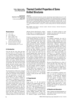


© Copyright 2026