1. sports
2. skating
3. figure skating

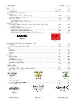
Commentariesare informative
essays dealingwithviewpointsof statisticalpractice,statisticaleducation, and othertopicsconsideredto
be of generalinterestto the board readershipof The AmericanStatistician.Commentariesare similarin spiritto Lettersto theEditor,but
theyinvolvelongerdiscussionsof background,issues, and perspectives. All commentarieswill be refereedfor their meritand compatibilitywiththese criteria.
How to Display Data Badly
HOWARD WAINER*
Methods for displayingdata badly have been developing formanyyears,and a wide varietyof interesting
and inventiveschemeshave emerged.Presentedhere is
a synthesisyieldingthe 12 most powerfultechniques
thatseem to underliemanyof the realizationsfoundin
practice.These 12 (the dirtydozen) are identifiedand
illustrated.
KEY WORDS: Graphics; Data display;Data density;
Data-ink ratio.
categorized. This article is the beginningof such a
compendium.
The aim of good data graphicsis to displaydata accuratelyand clearly.Let us use thisdefinitionas a starting
pointforcategorizingmethodsof bad data display.The
definitionhas threeparts. These are (a) showingdata,
(b) showing data accurately, and (c) showing data
clearly.Thus, ifwe wishto displaydata badly,we have
three avenues to follow. Let us examine them in sequence, parse themintosome oftheircomponentparts,
and see if we can identifymeans for measuringthe
success of each strategy.
2. SHOWING DATA
1. INTRODUCTION
The displayof data is a topic of substantialcontemporaryinterestand one thathas occupied the thoughts
of manyscholarsforalmost200 years.Duringthistime
there have been a numberof attemptsto codifystandards of good practice (e.g., ASME Standards 1915;
Cox 1978; Ehrenberg 1977) as well as a number of
books that have illustrated them (i.e., Bertin
1973,1977,1981; Schmid 1954; Schmid and Schmid
1979; Tufte 1983). The last decade or so has seen a
tremendousincreasein the developmentof new display
techniquesand tools thathave been reviewedrecently
(Macdonald-Ross 1977; Fienberg 1979; Cox 1978;
Wainer and Thissen 1981). We wish to concentrateon
methodsof data displaythatleave the viewersas uninformedas theywerebeforeseeingthedisplayor, worse,
those thatinduce confusion.Althoughsuch techniques
are broadlypracticed,to my knowledgetheyhave not
as yet been gatheredinto a single source or carefully
Obviously,if the aim of a good displayis to convey
information,
the less information
carriedin the display,
Change in Science Achievement of 9-,
13-,and 17-Year-Olds,by Type of
Exercise: 1969-1977
Changeinpercentcorrect
1,
O1
A
,,i,,,,
biologicalscience
_.
Physical
science
9-YEAR-OLDS
s ss
llll.|||
________
-2
-3
_
13-YEAR-OLDS
0I
-2
-3
_
-4
_5
*Howard Waineris Senior Research Scientist,Educational Testing
Service,Princeton,NJ08541. This is the textof an invitedaddressto
the AmericanStatisticalAssociation. It was supportedin partby the
ProgramStatisticsResearch Project of the Educational TestingService. The authorwould like to expresshis gratitudeto the numerous
friendsand colleagues who read or heard this article and offered
valuable suggestionsfor its improvement.Especially helpfulwere
David Andrews, Paul Holland, Bruce Kaplan, James 0. Ramsay,
Edward Tufte, the participantsin the StanfordWorkshopon Advanced Graphical Presentation,two anonymousreferees,the longassociate editor,and Gary Koch.
suffering
-6
-2
-h
-4
1969
Is_ _
1970
17-YEAR-OLDS
=
_ _ _ _ _ _ _ __ _ _ _ _
a
...............
...1
1_ _ _ _ _ __ _ _ _ _ _ _ _ _ _ _ _
1973
1977
Figure 1. An example ofa low densitygraph (fromS13 [ddi = .3]).
C) The AmericanStatistician,May 1984, Vol. 38, No. 2
137
Schools
PublicandPrivate
Elementary
Selected
Years1929-1970
m Public
-Prjvale
d0oi Schools
Thousan
0.8 F
300
2
i_
0.
-
0
t.4
0.0
0.6
LOCATION DIFFERENCE:
1929-30
1.0
0.Z
the worse it is. Tufte(1983) has devised a scheme for
in displays,called
measuringthe amountof information
the data densityindex (ddi), whichis "the numberof
numbersplotted per square inch." This easily calcuIn popular
informative.
lated indexis oftensurprisingly
and technicalmedia we have founda range from.1 to
362. This provides us with the firstrule of bad data
display.
jyy US.vsJapan
_~~~~~~~~~~~~~.
pe
r
mon-ho
urmQanus
in
15-
14 -
13C,,
Is
* 12C/
70%
62.3%/
ur
ngfn
cia
reta-oU
1930
1940
1950
1960
1970
10 _
upt
44%/
9
0"
Post)with
graph(? 1978,TheWashington
Figure3. Alowdensity
tofillinthespace (ddi = .2).
chart-junk
138
1969-70
THENUMBER
SCHOOLS
OFPRIVATE
ELEMENTARY
FROM1930-1970
What does a data graphicwitha ddi of .3 look like?
Shown in Figure 1 is a graphicfromthe book Social
IndicatorsIII (S13), originallydone in fourcolors (original size 7" by9") thatcontains18 numbers(18/63= .3).
The median data graphin S13 has a data densityof .6
thisone is notan unusualchoice. Shownin
numbers/in2;
Figure 2 is a plot fromthe article by Friedman and
Rafsky(1981) witha ddi of .5 (it shows4 numbersin 8
100%-moutpu
1959-60
in2).Thisis unusualforJASA,wherethemediandata
ofthis
graphhasa ddiof27. In defenseoftheproducers
plot,thepointofthegraphis to showthata methodof
analysissuggestedby a criticof theirpaperwas not
I suspectthatprosewouldhaveworkedpretty
fruitful.
wellalso.
canbe madethathighdatadenarguments
Although
willbe good,norone
sitydoes notimplythata graphic
of
on theefficiency
bad,itdoesreflect
withlowdensity
ifwe hold
ofinformation.
Obviously,
thetransmission
and accuracyconstant,
moreinformation
is betclarity
Rule 1-Show as Few Data as Possible (Minimize the
Data Density)
.00
1949-50
SchoolYear
Figure 4. Hidingthe data in the scale (fromS13).
3 JNIT
Figure 2. A low densitygraph (fromFriedmanand Rafsky1981
[ddi = .5]).
Labor
1939-40
1930
1940
1950
1960
9.275
10.000
10.375
13.574
14.372
1910
Figure5. Expandingthescale and showingthedata inFigure4
(from
S13).
(? The AmericanStatistician,
May 1984, Vol. 38, No. 2
A New Set ofProjectins forthe U.S. Supplyof Energy
Compared are two proctlons ot United State *rtrgy upply In th, y.r 2000 made by the Pftedynt s Council of
EnvirnonottalOuallty and th ectual
1977 supply Alltigurasar
* inquads
a
uunitaootm"aurmomntthat reprnt
millionbillin-on
quadrilion- Britlsh thettal unlts (8T U a), a standard masure otfergy
.
T0~~i_
tal 777
1977
M~~~~~~S
5
5_
/
2000 - AEr,ph
syes,egy
c_e,to
I
U
42 -14
-1
a
t
Nca,
Solad
'40
Total
1a
-
,l&U^,*
(inmillions
ofU S dollars)
3,000
6,000
U.S. exports
to China
4,000
U.S. exports
to Taiwan
U.S. imports
fromChina
1
9
2000
1,000
*
l
____
U.S. imports
fromTaiwan
2,000
19
2000-8
Erphas.zes.rc,eased
37d
erergyoduct.on
1.:
Cmnlions ofU.S dollars)
Coal
'
Tutal 05
7 7 7)
O.la,daa*
.N
(1979 The New York Times
Figure 6. Ignoringthe visual metaphor (? 1978, The New York
Times).
ter than less. One of the great assets of graphical techniques is that theycan convey large amounts of information in a small space.
We note that when a graph contains littleor no information the plot can look quite empty (Figure 2) and
thus raise suspicions in the viewer that there is nothing
to be communicated. A way to avoid these suspicions is
to fill up the plot with nondata figurations-what Tufte
has termed "chartjunk." Figure 3 shows a plot of the
labor productivity of Japan relative to that of the
United States. It contains one number for each of three
years. Obviously, a graph of such sparse information
would have a lot of blank space, so filling the space
hides the paucity of information from the reader.
A convenient measure of the extent to which this
practice is in use is Tufte's "data-ink ratio." This measure is the ratio of the amount of ink used in graphing
the data to the total amount of ink in the graph. The
closer to zero this ratio gets, the worse the graph. The
notion of the data-ink ratio brings us to the second
principle of bad data display.
Rule 2-Hide WhatData You Do Show
(MinimizetheData-Ink Ratio)
One can hide data in a variety of ways. One method
that occurs with some regularityis hiding the data in the
grid. The grid is useful for plotting the points, but only
rarely afterwards.Thus to display data badly, use a fine
grid and plot the points dimly (see Tufte 1983,
pp. 94-95 for one repeated version of this).
A second way to hide the data is in the scale. This
corresponds to blowing up the scale (i.e., looking at the
data from far away) so that any variation in the data is
obscured by the magnitude of the scale. One can justify
this practice by appealing to "honesty requires that we
start the scale at zero," or other sorts of sophistry.
In Figure 4 is a plot that (from S13) effectivelyhides
the growth of private schools in the scale. A redrawing
of the number of private schools on a differentscale
conveys the growththat took place duringthe mid1950's (Figure5). The relationshipbetweenthisriseand
Brownvs. TopekaSchoolBoardbecomes an immediate
question.
To conclude thissection,we have seen thatwe can
displaydata badlyeitherbynotincludingthem(Rule 1)
1972
1974
1976
1978
1980
1970
1972
1974
1976
1978
1980
Source DpartmentofCommerce
Figure 7. Reversing the metaphorin mid-graphwhilechanging
scales on both axes (? June 14, 1981, The New YorkTimes).
or by hidingthem(Rule 2). We can measuretheextent
to whichwe are successfulin excludingthedata through
the data density;we can sometimesconvince viewers
that we have included the data throughthe incorporationof chartjunk.Hidingthe data can be done either
by usingan overabundanceof chartjunkor by cleverly
choosingthe scale so thatthe data disappear. A measure of the success we have achieved in hidingthe data
is throughthe data-inkratio.
3. SHOWING DATA ACCURATELY
The essence of a graphicdisplayis thata set of numbers havingboth magnitudesand an order are represented by an appropriatevisual metaphor-the magnitude and order of the metaphoricalrepresentation
matchthenumbers.We can displaydata badlybyignoring or distortingthisconcept.
Rule 3-Ignore the Visual MetaphorAltogether
If the data are orderedand ifthevisualmetaphorhas
a naturalorder,a bad displaywill surelyemergeifyou
shufflethe relationship.In Figure 6 note thatthe bar
labeled 14.1 is longerthanthe bar labeled 18. Another
methodis to changethemeaningofthemetaphorin the
middleof the plot. In Figure7 the dark shadingrepresentsimportson one side and exportson theother.This
is but one of the problemsof thisgraph; more serious
stillis the change of scale. There is also a differencein
the timescale, but thatis minor.A commonthemein
Playfair's(1786) work was the differencebetweenimports and exports. In Figure 8, a 200-year-oldgraph
tellsthe storyclearly.Two such plots would have illustratedthe storysurroundingthis graph quite clearly.
Rule 4-Only Order Matters
One frequenttrickis to use lengthas thevisualmetaphorwhenarea is whatis perceived.Thiswas used quite
effectively
by The WashingtonPost in Figure 9. Note
thatthisgraphalso has a low data density(.1), and its
data-inkratio is close to zero. We can also calculate
Tufte's (1983) measure of perceptual distortion(PD)
forthisgraph.The PD in thisinstanceis the perceived
?) The AmericanStatistician,May 1984, Vol. 38, No. 2
139
C IIA ItTT
& 1511'01TS8I
E-xPORT.i
rLA_A
E-.N;
C_
~
.........
.
-
~
~
~
~
~
5tf
.
eariler(from
1786).
Playfair
Figure8. A ploton thesame topicdone welltwocenturies
to
changein thevalueof thedollarfromEisenhower
Carterdividedbytheactualchange.I readandmeasure
thus:
Til E tIXITEI, S1A'M1IS,
(WFAMIEICiA.A
E 1430I3632
Measured
Actual
U5
5
1.00- .44
=44 1.27
5
PD = 9.68/1.27= 7.62
1958- ESENHOWER:
$1.
TiE
FAtV '
butby no
This distortion
of over700% is substantial
meansa record.
A less distorted
viewof thesedata is providedin
Figure10. In addition,the spacingsuggestedby the
0
94c
1963 - KENNEDY:
pw~~~~~~~~~~~
E I SENHOWER
KENNE
DT
JOHNSON
t
4
362tX
0.8
1968- JOHNSON:53Uc
IN:
22.00- 2.06
96
2.06
I 1TEDISTA\TE:SM'A3.11:11
.
_
~0. 4
=0.2
CC
ofthel
lXnlshllng r4 ffiN^>:
0.2
Dollar
rc:LuborDportment
0. O.I
44CAR
1978-CTER:
(August)
Figure 9. An example of how to goose up the effectby squaring
the eyeball (? 1978, The WashingtonPost).
140
I
1958
1963
1968
YERR
1973
I
1978
Figure10. Thedata inFigure9 as an unadornedlinechart(from
Wainer,1980).
? The AmericanStatistician,
May 1984, Vol. 38, No. 2
presidentialfaces is made expliciton the time scale.
Rule 5-Graph Data Out of Context
Often we can modifythe perceptionof the graph
(particularlyfortimeseriesdata) by choosingcarefully
theintervaldisplayed.A precipitousdropcan disappear
if we choose a startingdate just afterthe drop. Similarly,we can turnslightmeandersintosharpchangesby
focusingon a singlemeanderand expandingthe scale.
but can have proOftenthe choice of scale is arbitrary
of
foundeffectson theperception thedisplay.Figure11
shows a famous example in which PresidentReagan
viewof theeffectsof histax cut.
givesan out-of-context
The Times'alternativeprovidesthecontextfora deeper
understanding.Simultaneouslyomittingthe contextas
well as any quantitativescale is the keyto the practice
of Ordinal Graphics(see also Rule 4). Automaticrules
do not always work, and wisdom is always required.
In Section3 we discussedthreerulesforthe accurate
displayofdata. One can compromiseaccuracybyignoringvisual metaphors(Rule 3), byonlypayingattention
to the order of the numbersand not theirmagnitude
(Rule 4), or by showingdata out of context(Rule 5).
We advocated the use of Tufte'smeasureof perceptual
distortionas a wayof measuringtheextentto whichthe
accuracyof the data has been compromisedby the disthatwouldallow it
play. One can thinkof modifications
to be applied in other situations,but we leave such
expansion to otheraccounts.
4. SHOWING DATA CLEARLY
In this section we discuss methods for badly displayingdata that do not seem as serious as those deYORK
THE NEW
TIMES,
Paymentsunderthe
Ways and Means
Committeeplan
$2500
2000
1 ???
w
$
NEWS
1,829,000
;
1,636,000
2000
%
1,500,000(-
INCOME
-
...
1986
$
1,555,000
-
S20.000
1982
11W0
m
The soaraway Post
the daily paper
New Yorkers trust
1 700,000
AVERAGE FAMILY
by
SOfl4Nfl~
York Post compared to the plummetingDaily News
circulation.The reason given is that New Yorkers
"trust"the Post. It takesa carefullook to note the
700,000jump thatthe scale makesbetweenthe two
lines.
In Figure13 is a plot of physicians'
incomesover
time.It appearsto be linear,witha slighttapering
off
inrecentyears.A carefullookat thescaleshowsthatit
starts
outplotting
everyeightyearsandendsupplotting
yearly.A moreregularscale(in Figure14) tellsquitea
different
story.
1,800000
$2500
YOUR TAXES
Tawpld
Thisis a powerful
techniquethatcan makelargediflooksmallandmakeexponential
ferences
changeslook
linear.
In Figure12 is a graphthatsupportstheassociated
storyabout the skyrocketing
circulation
of The New
__
Paymentsundr the
Prdentfs proposW
1500
Rule 6-Change Scales in Mid-Axis
1,900,000.
2, 1981
SUNDAY, AUGUST
thatis, thedata are displayed,
scribedpreviously;
and
theymight
evenbe accurateintheirportrayal.
Yetsubtle(and notso subtle)techniques
can be usedto effectivelyobscurethe mostmeaningful
or interesting
aspectsofthedata.Itismoredifficult
toprovideobjective
measuresof presentational
clarity,
butwe relyon the
readerto judgefromtheexamplespresented.
bu,000
-
1,491,000
-
THEIR
~~~~~~~BILL
500l
OUR
...
BILL
k00t0
-
E~~~17
.:_
Fiur 12. Chngn
1982
1983
1984
1985
.scl
-_
197
__
198
~
a., :a1....
198
1982_-- .-E
inmid-ai tomak lag differences.
198
scale norcontext
Figure11. The WhiteHouse showingneither
withpermission).
(? 1981,The NewYorkTimes,reprinted
May 1984, Vol. 38, No. 2
? The AmericanStatistician,
141
ofDoctors
hIcomes
Vs.Other
Profesionals
(MEDIANNETINCOMES)
Median Income of Year-Round, Full-Time
Workers 25 to 34 Years Old, by Sex and
Educational Attainment:1961977
Constant 1977 dollars
$20,000
$18000
SOURCE:Council
onWageandPrice
Stability
54,14
5,4
1i 50,823
_
_,
~~,
I~--
,_~_
_s
r
-
$8,000
-
$4,000
-
$2,000
25,050
years or
6to16
M
~
...
$14,001
A
$ l0
1951 1955
1963 1965 1967 1970 1972 1973 1974 1975 1976
Figure 13. Changingscale inmid-axistomake exponentialgrowth
linear (? The WashingtonPost).
Rule 7-Emphasize the Trivial(Ignore theImportant)
Sometimesthe data thatare to be displayedhave one
importantaspect and othersthatare trivial.The graph
can be made worse by emphasizingthe trivialpart. In
Figure 15 we have a page fromS13 that compares the
incomelevels of men and womenby educationallevels.
It reveals the not surprisingresultthatbettereducated
individualsare paid betterthan more poorlyeducated
ones and thatchangesacrosstimeexpressedin constant
dollars are reasonably constant. The comparison of
greatestinterestand currentconcern, comparingsalaries between sexes withineducation level, must be
made clumsilyby verticallytransposingfromone graph
to another.It seems clear that Rule 7 musthave been
operatinghere,forit would have been easy to place the
graphsside byside and allow the comparisonofinterest
to be made more directly.Looking at theproblemfrom
a strictly
data-analyticpointof view, we note thatthere
are two large main effects(education and sex) and a
small time effect.This would have implied a plot that
INCOMES OF DOCTORS VS.
-__-
-ale'
-
-|--
effct
~a own,
larges
_ _
_
-
clal
-
pla
a
Feor
$4,000
-
_ _
$2,0 0 0
_ _
_ _
_ _
__
_ _
_ _
_
$0
1968
-
_ _
_ _
_ _
-
-
an
$1,000
9
-
_ _
lees
1970
1972
1974
_ _
_ _
__
_ _
_ _
1976
1978
S13).
showedthe large effectsclearlyand placed the smallish
timetrendinto the background(Figure 16).
110
12_1`1F ,IA,A
1
'1
20-
Males
16
C"
12
~MalesV
-
Females
4
1964
1969
-maximum
-median
(uveriime)
STRRTE0
n010.
1974
YEAR
Figure14. Data fromFigure13 redonewithlinearscale (from
Wainer1980).
C) The AmericanStatistician,May 1984, Vol. 38, No. 2
~~~~~~~~~~~~~~~Female
-'
Legend
z30/
1959
e
MEDIAN
INCOME
OFYEAR-ROUND
FULL
TIME
WORKERS
25-34YEARS
OLDBYSEXANDEDUCATIONAL
ATTAINMENT:
1968-1977
1977DOLLARS)
(INCONSTANT
8
1954
1980
differencesin income throughthe verticalplacement ofplots (from
PROFESSIONALS
1949
y ars
_
thetrivial:
ofsex
Hidingthemaineffect
Figure15. Emphasizing
DOCTORS
OTHER
19414
-
ic
20
OTHER PROFESSIONRLS
H~~~~~~~~~~~EOICRRE
d-
eard
thessals
o
_ _
I--
142
_
-
SW_L71V
-
showed~~
-60
cso
1939
ein meo
ino
2
1 year
_
_
710
z
ore
13 ro 1,5yeror
--
8,744
z20
2
=
16,107
$3,262
n50
=
--LIL16eaorm
s__
-_
>_ __ _
$1200
34,740
=
_|
~~~
____
~
-n
=
$10,0000
46,780
1939 1947
s_
~~~~
~~
mm
L
A__
$12,000
43,100
13,150
?
=
$16000 _
62.799
-
.
$14,000
OFFICED-BASED
NONSALARIEDPHYSICIANS
MALE
-
BIL. LB.
2.5
LAMB
MUTTON
........ . ...
1.5
....... ......
Canada, 1970-1972
--- -
1.0-...:
- AN
. .;; ' : .: : :: : ',::
BEEF
-:...
o~~~~~~~.'.:;::-:
0.
.;....
VEAL
....: ..
::.;.
Finland,1974
.: ,- :. ' : : : : : : :;
..,...,...;
'X'-*
....,,.;.-France,1972
1960
Female
HIM
Austria,1974 1975
' , ,\ : : :, :
Female
AND GOATMEAT
2.0
1 N.
0 ' N":
m Male
LifeExpectancy at Birth,by Sex, Selected
Countres, Most Recent Available Year:
1970-1IMi
U.S. IMPORTS OF RED MEATS
1963
i90
1969
1972
1975
1978
Germany(Fed Rep ,
^~~~~~~~~~~~~~~~~~~~~~~~~~a
1973-1975
FA
*eAftcA WG, r EOUIVALENT
1
'.:,:
ill i
-:-@:-:-:9o
Figure 17. Jigglingthebaseline makes comparisonsmore difficult
4
|
R
l
Japan, 1974
Charts).
(fromHandbookofAgricultural
U S S R., 1971-1972)
i
S
S
Rule 8-Jiggle theBaseline
Making comparisonsis alwaysaided when the quantitiesbeingcomparedstartfroma commonbase. Thus
we can alwaysmake the graphworse by startingfrom
differentbases. Such schemes as the hangingor suspended rootogramand the residual plot are meant to
facilitatecomparisons.In Figure 17 is a plot of U.S.
importsof red meat takenfromthe Handbook of AgriculturalChartspublishedby the U.S. Departmentof
Agriculture.Shadingbeneatheach line is a convention
thatindicatessummation,tellingus thatthe amountof
each kind of meat is added to the amounts below it.
Because of the dominance of and the fluctuationsin
importationof beef and veal, it is hard to see whatthe
changesare in theotherkindsof meat-Is the importation of porkincreasing?Decreasing? Stayingconstant?
The onlypurposeforstackingis to indicategraphically
the total summation.This is easily done throughthe
addition of another line for TOTAL. Note that a
TOTAL willalwaysbe clear and willneverintersectthe
otherlineson theplot. A versionof thesedata is shown
U.S. IMPORTS OF RED rMEATS*
BIL. LB.-
2.5 e-_____~~_
POkK
101960
Source:
Chart
1963
1966
1969
Charts ,
Handbook of Agri_ultural
1976, p. 93.
Agriculture,
Source:
1972
U.S .
1978
1975
Department
of
Origzinal
line
versionofFigure17 witha straight
Figure18. Analternative
used as thebasis ofcomparison.
Sweden, 1971-1975
UnitedKingdom,1970-1972
UnitedStates, 1975
0
50
60
70
80
90
Years of lifeexpectancy
Figure 19. AustriaFirst!Obscuring the data structureby alphabetizingthe plot (fromS13).
in Figure18 withtheseparate amountsof each meat,as
well as a summationline, shown clearly. Note how
easily one can see the structureof importof each kind
of meat now that the standard of comparison is a
straightline (the time axis) and no longerthe import
amountof those meats withgreatervolume.
Rule 9-Austria First!
Ordering graphs and tables alphabeticallycan obin thedata thatwouldhave been obvious
scurestructure
had the display been ordered by some aspect of the
data. One can defend oneself against criticismsby
pointingout thatalphabetizing"aids in findingentries
of interest."Of course,withlistsof modestlengthsuch
aids are unnecessary;with longer lists the indexing
schemescommonin 19thcenturystatisticalatlases provide easy lookup capability.
Figure 19 is anothergraphfromSf3 showinglifeexpectancies,dividedby sex, in 10 industrializednations.
The order of presentationis alphabetical (with the
USSR positionedas Russia). The messagewe getis that
thereis littlevariationand thatwomenlive longerthan
men. Redone as a stem-and-leafdiagram(Figure 20 is
simplya reorderingof the data with spacing proportional to the numericaldifferences),the magnitudeof
leaps out at us. We also note thatthe
the sex difference
USSR is an outlierformen.
Rule JO-Label (a) Illegibly,(b) Incompletely,
and (d) Ambiguously
(c) Incorrectly,
There are manyinstancesof labels thateitherdo not
C) The AmericanStatistician,May 1984, Vol. 38, No. 2
143
LIFE EXPECTANCYAT BIRTH, BY SEX,
MOST RECENTAVAILABLEYEAR
YEARS
WOMEN
SWEDEN
FRANCE, US, JAPAN, CANADA
FINLAND, AUSTRIA, UK
USSR,GERMANY
78
77
76
75
74
73
72
71
70
69
68
67
66
65
64
673
62
r3Ef
Commtssion
Payqrents
to Travel Agents
15o
m
L
1 20-
L
JUNITE
I
SWEDEN
JAPAN
0
N
CANADA,UK,US, FRANCE
GERMANY,AUSTRIA
FINLAND
9 0-
TWA
5
E A S TERN
0
F
60D ELTA
D
0
USSR
L
30-
L
I
Figure 20. Orderingand spacing the data fromFigure 19 as a
stem-and-leaf diagram provides insights previously difficultto
extract(fromS13).
A
R
5
0
1976
tell the whole story,tell the wrongstory,tell two or
more stories,or are so small thatone cannotfigureout
whatstorytheyare telling.One ofmyfavoriteexamples
of small labels is fromThe New York Times (August
1977
1978
(ea
t I ma t e d
Y EAR
Figure 22. Figure 21 redrawn with 1978 data placed on a
comparable basis (fromWainer1980).
1978), in whichthearticlecomplainsthatfarecutslower
commissionpaymentsto travelagents.The graph(Figure 21) supportsthisviewuntilone noticesthetinylabel
indicatingthatthe small bar showingthe decline is for
just the firsthalfof 1978. This omitssuch heavytravel
periodsas Labor Day, Thanksgiving,
Christmas,and so
on, so thatmerelydoublingthe first-half
data is probablynot enough. Nevertheless,whenthisbar is doubled
(Figure 22), we see thatthe agentsare doingverywell
indeed comparedto earlieryears.
ToTravel
Agents
In lkosoldofdlAer
$57~~~~~~~~~~~~~~~'6
Rule 11-More Is Murkier:(a) More Decimal
Places and (b) More Dimensions
O
web
~~E,ASTIEEN
discount
of
d
and airlines' telephone
unITE=D
s
areras
fars
(ravel agents'overhead,offsetting
revenuegainsfromhighervolume.
Figure21. Mixing
a changedmetaphor
witha tiny
labelreverses
themeaningofthedata (? 1978,The NewYorkTimes).
144
We oftensee tables in whichthe numberof decimal
places presentedis farbeyondthe numberthatcan be
perceived by a reader. They are also commonly
presentedto show more accuracythan is justified.A
displaycan be made clearerbypresentingless. In Table
1 is a sectionof a table fromDhariyal and Dudewicz's
(1981) JASA paper. The table entriesare presentedto
five decimal places! In Table 2 is a heavilyrounded
versionthatshowswhatthe authorsintendedclearly.It
also shows thatthe variouscolumnsmighthave a substantialredundancyin them (the maximumexpected
gain withb/c = 10 is about 1/10ththatof b/c = 100 and
1/100th
thatof b/c = 1,000). If theydo, theentiretable
could have been reduced substantially.
Justas increasingthe numberof decimal places can
make a table harderto understand,so can increasing
the number of dimensionsmake a graph more con-
(C The AmericanStatistician,May 1984, Vol. 38, No. 2
Table 1. OptimalSelection Froma Finite
Sequence WithSampling Cost
b/c = 10.0
N
r*
3
4
5
6
7
8
9
10
2
2
2
3
3
3
3
4
100.0
(GN(r*) - a)/c
.20000
.26333
.32333
.38267
.44600
.50743
.56743
.62948
1,000.0
r*
(GN(r*) - a)/c
r*
(GN(r*) - a)/c
2
2
3
3
3
4
4
4
2.22500
2.88833
3.54167
4.23767
4.90100
5.57650
6.26025
6.92358
2
2
3
3
3
4
4
4
22.47499
29.13832
35.79166
42.78764
49.45097
56.33005
63.20129
69.86462
NOTE: g(Xs + r - 1) = bR(Xs + r - 1) + a, ifS =s, and g(Xs +r - 1)= 0, otherwise.
Source: Dhariyaland Dudewicz (1981).
fusing.We have alreadyseen how extradimensionscan
cause ambiguity(Is it lengthor area or volume?). In
addition, human perceptionof areas is inconsistent.
Justwhatis confusingand whatis notis sometimesonly
a conjecture,yet a hintthat a particularconfiguration
willbe confusingis obtainedifthe displayconfusedthe
grapher.Shownin Figure23 is a plot of per shareearningsand dividendsovera six-yearperiod. We note (with
some amusement)that 1975 is the side of a bar-the
third dimension of this bar (rectangular parallelopiped?) charthas confusedtheartist!I suspectthat1975
is reallywhatis labeled 1976, and the unlabeled bar at
the end is probably1977. A simpleline chartwiththis
interpretation
is shownin Figure 24.
In Section4 we illustratesix morerulesfordisplaying
data badly. These rulesfall broadlyunderthe heading
of how to obscurethe data. The techniquesmentioned
were to change the scale in mid-axis,emphasize the
trivial,jiggle the baseline, orderthe chartby a characteristicunrelatedto the data, label poorly,and include
more dimensionsor decimalplaces thanare justifiedor
needed. These methodswillworkseparatelyor in combinationwith othersto produce graphs and tables of
littleuse. Their commoneffectwill usuallybe to leave
the reader uninformedabout the points of interestin
the data, althoughsometimestheywill misinformus;
the physicians'incomeplot in Figure 13 is a primeexample of misinformation.
Finally,the availabilityof color usually means that
there are additionalparametersthat can be misused.
The U.S. Census' two-variablecolor map is a wonderful
example of how using color in a graph can seduce us
Table 2. OptimalSelection Froma FiniteSequence
WithSampling Cost (revised)
b/c = 10
b/c = 100
b/c = 1,000
N
r*
G
r*
G
r*
G
3
2
.2
2
2.2
2
22
4
2
.3
2
2.9
2
29
5
6
7
8
9
10
2
3
3
3
3
4
.3
.4
.4
.5
.6
.6
3
3
3
4
4
4
3.5
4.2
4.9
5.6
6.3
6.9
3
3
3
4
4
4
NOTE:g(Xs + r- 1) =bR(Xs + r - 1) + a, ifS = s, andg(Xs + r - 1)
intothinkingthatwe are communicating
more thanwe
are (see Fienberg 1979; Wainer and Francolini1980;
Wainer 1981). This leads us to the last rule.
Rule 12-If It Has Been Done Wellin thePast, Thinkof
AnotherWayto Do It
The two-variablecolor map was done ratherwell by
Mayr(1874), 100 yearsbeforethe U.S. Census version.
He used bars of varyingwidthand frequencyto accomplish gracefullywhat the U.S. Census used varying
saturationsto do clumsily.
A particularlyenlighteningexperience is to look
carefullythroughthe six books of graphsthatWilliam
Playfairpublished duringthe period 1786-1822. One
discoversclear, accurate, and data-laden graphs containingmanyideas thatare usefuland too rarelyapplied
today. In the course of preparingthis article,I spent
manyhours lookingat a varietyof attemptsto display
Earns g~~~
PerSha LAnd
DMndenldxs
(Dollars)
1.71
111.
1.21.70
1.63
1.53
S
I ,.S
L....I
<
m
.
Earning
1~~~.....'.. ',.
-:-
... '' .. .....1
D......d.
Figure,"'.''.
23'.'''.
An extra
.. .
.:::
, :.:.:
.: ::::::.:;:;:
'' :..:.:.
. . ...
:: . . :.
::::::..:
: :::
. . ::.. .::::
.::.:
:. .: ::::::
.:
.
.
.cnueevnt
.
.
~::" ~.:::. '~ ~dimensn..
: :.: :, .:
: :"',.. .:
.. .;;:.
. .
( : 1979,::::The Washington
Post)::.::::::
::
: . . :.'. :: .:- . :.. . : '. . ' .:::
::::::::
:::::::::;:::~
:
.'
.: . .:::::
~~~~~~~~~~.,.
:'.::'..
:. . :.. '
.,:.. . .
':~~~~~~~~~~~
.. . . . . . .
'.,...::~
. . . . . . . .
. . . . . . . .
.:::::
.
..
.:::
....
.:::: ..... . .::
::
::
.:
.::::::::
:
.:
.:::
:::
Fiur
.t .99
.:::::::::::::::
.:
.: . ; . : .:
::
::
::.:..
..:: .::
:..
. :. : . ,''
...
.': . ". '.
.:
:
:::
.:: .::::::.
:: :::
.: . .. . .. . .
. .::.. .' . . :.'::
. . . . . . ..
. . . . . . .
.''
.:'
. ~~ .::
~~~~~~
": . .':
.,.,
,,,.,
...,., .::::::''
X~~~~~~~~~~~~~~~~~~~~~~~~~~~~~
73
972~~~~~~~~~~~~.
... .6.77 7S
......
l . .Dvded
1
.l
gr
..
;:::::::
. . . .
:.: . .: :::
.:
.. . .
:.' ,. ,. ,.::"
'::"
~~~~~~~~~~~~
.:
..
.:
: . . :'. .: .........
.4.
,.
.
,.....................
:':'
.. ...
..
.
Eanig
An.h
xr
2. . .ieso
Wahngo
.h .Post)....
cofue .grapher .eve
....
..
....
...
36
43
49
56
63
70
0, otherwise.
?D The AmericanStatistician,May 1984, Vol. 38, No. 2
145
2. 00
Beginning at the left on the Polish-Russian border near the
Nieman River,the thickband showsthe size of the army(422,000
men) as it invaded Russia in June 1812. The widthof the band
indicatesthe size of the armyat each place on the map. In September,the armyreached Moscow, whichwas by thensacked and
deserted,with100,000men. The path of Napoleon's retreatfrom
Moscow is depictedby the darker,lowerband, whichis linkedto
a temperaturescale and dates at the bottomof the chart.It was a
bitterlycold winter,and manyfrozeon the marchout of Russia.
As the graphicshows, the crossingof the Berezina River was a
disaster,and the armyfinallystruggledback to Poland withonly
10,000menremaining.Also shownare themovementsof auxiliary
troops, as theysought to protectthe rear and flankof the advancingarmy.Minard'sgraphictellsa rich,coherentstorywithits
thanjust a singlenumber
multivariate
data, farmore enlightening
bouncingalong over time.Six variablesare plotted:the size of the
surface,directionof the
army,its location on a two-dimensional
army'smovement,and temperatureon various dates duringthe
retreatfromMoscow.
It may well be the best statisticalgraphicever drawn.
1. 75
EornL n.
I . 50
cca
-J
M
1.25
Di vXdend.
1.00
1972
1976
1974
Y E RR
Figure 24. Data fromFigure 23 redrawn simply (fromWainer
1980).
5. SUMMING UP
data. Some of the horrorsthat I have presentedwere
the fruitsof thatsearch. In addition,jewels sometimes
emerged. I saved the best for last, and will conclude
withone of those jewels-my nominee forthe titleof
"World's Champion Graph." It was produced by
Minard in 1861 and portraysthe devastatinglosses sufferedby the Frencharmyduringthe course of Napoleon's ill-fatedRussian campaign of 1812. This graph
(originallyin color) appears in Figure 25 and is reproducedfromTufte'sbook (1983, p. 40). His narrative
follows.
Althoughthe tone of thispresentationtended to be
lightand pointed in the wrong direction,the aim is
serious. There are manypathsthatone can followthat
willcause deteriorating
qualityof our data displays;the
12 rules that we described were only the beginning.
Nevertheless,theypointclearlytowardan outlookthat
providesmanyhintsforgood display.The measuresof
display described are interlocking.The data density
cannotbe highifthe graphis clutteredwithchartjunk;
the data-inkratio growswiththe amount of data displayed; perceptualdistortionmanifestsitselfmost fre-
dans la campagnede Russ\e1812-1813.
CARTE FIGURATIVE des pertes successivesen hommesde l Armnee
Franr&ise
Ceneralt de. Ponts et Chausseesen retra'cte.
Dresscepar M.Mtnard.
Inspecteur
C,~~~~~~~~~~~~~~~~~~~~~~~~~~~~~~~
0
0t'r''
=
6I)7ollzhtr
e~~~~~~~~~
=I
Awer
G.&'&-
j
0
- 2 0 1. Z 8 9 1 "
-tie-,
-
146
Mnar'sTABLE
-
-
I )cc:iibtr
-
ofthis0initsoriginalcolor-p.176).
q_ superb_
reproduction
Tufte_
1983_
Fiue
5 for_inr'
(81)gah
fte
rnc ry' l-ftd oa it
Tufe183for~ upeb eprducio ofths i is oigialcolr-.
16)
Figue 2.
gaUho
tRAhe Urenh Army'sil-ftued
Z~~~~~~~~~~~~~~~*~~~~~~~~*~~~~~~~
9b~~~~~~~~~~~~~~~.
5$~~~~~~~~~~~~C
--
~~~~~~~~~~~~~~~~~
XIr
=
,
N'~~~ciubcr
usi-Acnidt
deRedusieoa nt
C The AmericanStatistician,
May 1984, Vol. 38, No. 2
- - _ _ _ _ _ _ _ _ _ _ _ _r._ _ _ _ _ _ _ _ _ _ _ _ _ _ _ _ _ _ _
carmn~rdiae
-
orte il o Wrl'
10~~~~~~
October
CaponGah"(e
foa~r
the ditesouf deWorldsCapo
rp"(e
quentlywhenadditionaldimensionsor worthlessmetaphorsare included.Thus, therulesforgood displayare
quite simple. Examine the data carefullyenough to
know what theyhave to say, and then let them say it
witha minimumof adornment.Do thiswhilefollowing
reasonableregularity
practicesin thedepictionof scale,
and label clearlyand fully.Last, and perhapsmostimportant,spend some time looking at the work of the
mastersof the craft.An hour spent with Playfairor
Minard will not only benefityour graphicalexpertise
but will also be enjoyable. Tukey (1977) offers236
graphsand littlechartjunk.The workofFrancisWalker
(1894) concerningstatisticalmaps is clear and concise,
and it is trulya mysterythattheircurrentcounterparts
do not make betteruse of the schemadeveloped a centuryand more ago.
[ReceivedSeptember1982. RevisedSeptember1983.]
REFERENCES
BERTIN, J. (1973), Semiologie Graphique (2nd ed.), The Hague:
Mouton-Gautier.
(1977), La Graphique et le TraitementGraphique de
l'Information,France: Flammarion.
(1981), Graphicsand theGraphicalAnalysisof Data, translation, W. Berg, tech. ed., H. Wainer,Berlin: DeGruyter.
COX, D.R. (1978), "Some Remarks on the Role in Statisticsof
Graphical Methods," Applied Statistics,27, 4-9.
DHARIYAL, I.D., and DUDEWICZ, E.J. (1981), "Optimal Selection From a FiniteSequence WithSamplingCost," Journalof the
AmericanStatisticalAssociation,76, 952-959.
EHRENBERG, A.S.C. (1977), "Rudimentsof Numeracy,"Journal
of theRoyal StatisticalSociety,Ser. A, 140, 277-297.
FIENBERG, S.E. (1979), Graphical Methods in Statistics, The
AmericanStatistician,
33, 165-178.
FRIEDMAN, J.H., and RAFSKY, L.C. (1981), "Graphics forthe
MultivariateTwo-SampleProblem,"Journalof theAmericanStatisticalAssociation,76, 277-287.
JOINT COMMITTEE
ON STANDARDS
FOR GRAPHIC
PRESENTATION, PRELIMINARY REPORT (1915), Journal
of theAmericanStatisticalAssociation, 14, 790-797.
MACDONALD-ROSS, M. (1977), "How NumbersAre Shown: A
Review of Research on the Presentationof QuantitativeData in
Texts," Audiovisual CommunicationsReview,25, 359-409.
MAYR, G. VON (1874), "Gutachen Uber die Anwendungder Graphischenund Geographischen,"Methodin der Statistik,Munich.
MINARD, C.J. (1845-1869), Tableaus Graphiqueset CartesFigurativesde M. Minard,Bibliothequede l'Ecole Nationale des Pontset
Chaussees, Paris.
PLAYFAIR, W. (1786), The Commercialand PoliticalAtlas, London: Corry.
SCHMID, C.F. (1954), Handbook of Graphic Presentation,New
York: Ronald Press.
SCHMID, C.F., and SCHMID, S.E. (1979), Handbook of Graphic
Presentation(2nd ed.), New York: JohnWiley.
TUFTE, E.R. (1977), "ImprovingData Display," University
of Chicago, Dept. of Statistics.
(1983), The Visual Display of QuantitativeInformation,
Cheshire,Conn.: Graphics Press.
TUKEY, J.W. (1977), ExploratoryData Analysis,Reading, Mass:
Addison-Wesley.
WAINER, H. (1980), "Making Newspaper Graphs Fit to Prinit,"in
Processingof Visible Language, Vol. 2, eds. H. Bouma, P.A.
Kolers, and M.E. Wrolsted,New York: Plenum, 125-142.
, "Reply" to Meyerand Abt (1981), TheAmericanStatistician,
57.
(1983), "How Are We Doing? A Review of Social Indicators
III," Journalof theAmericanStatisticalAssociation,78, 492-496.
WAINER, H., and FRANCOLINI, C. (1980), "An Empirical InquiryConcerningHuman Understandingof Two-VariableColor
Maps," The AmericanStatistician,34, 81-93.
WAINER, H., and THISSEN, D. (1981), "Graphical Data Analysis,"Annual Reviewof Psychology,32, 191-241.
WALKER, F.A. (1894), Statistical
Atlas of theUnitedStatesBased on
theResultsoftheNinthCensus,Washington,D.C.: U.S. Bureau of
the Census.
?) The AmericanStatistician,May 1984, Vol. 38, No. 2
147