
Fire Ecology and Fire Effects USDA Forest Service Proceedings RMRS-P-41. 2006. 547
Fire Ecology and Fire Effects
USDA Forest Service Proceedings RMRS-P-41. 2006.
547
548
USDA Forest Service Proceedings RMRS-P-41. 2006.
Integrating Fuel Treatments into
Comprehensive Ecosystem Management
Kevin Hyde1, Greg Jones2, Robin Silverstein3, Keith Stockmann4, and
Dan Loeffler5
Abstract—To plan fuel treatments in the context of comprehensive ecosystem management, forest managers must meet multiple-use and environmental objectives, address
administrative and budget constraints, and reconcile performance measures from
multiple policy directives. We demonstrate a multiple criteria approach to measuring
success of fuel treatments used in the Butte North Strategic Placement of Treatments
(SPOT) pilot project. Located in the Beaverhead – Deerlodge National Forests, Montana, the project addresses multiple issues: altered wildlife habitat affecting sensitive
species, grassland conversion to forest, an insect epidemic, water resource concerns,
wildland-urban interface development, and wildland fire management. Managers are
working with researchers to develop dynamic landscape management strategies. They
employ multiple modeling approaches to conduct an integrated assessment of ecological and resource issues relative to multiple management scenarios. Besides evaluating
effects of proposed treatments on changes to fire behavior, they also evaluate effects
on wildlife habitat, disturbance processes, water quality and economics of treatment
alternatives. The intent is to effectively integrate fuel management with Forest Plan
goals and comprehensive ecosystem management. This approach offers a structure to
use multiple criteria to evaluate success of fuel management activities in the context
of other resource objectives.
Introduction
Recent dramatic increases in wildland fi res triggered the commitment of
substantial resources to reduce hazardous fuels. The Government Accounting
Office (2002) calls for federal land management agencies to develop “consistent criteria to identify and prioritize” areas requiring treatment and “clearly
defi ned outcome-oriented goals and objectives.” The urgency to reduce forest
fuels creates tension with expectations that forest management must address
competing resource objectives while applying the best available ecosystem
science. The Healthy Forest Restoration Act of 2003 established a framework
to conduct hazardous fuels reduction projects on federal forested lands to
protect key ecosystem components, reduce risk to communities and municipal
water supplies, improve critical habitat for threatened or endangered species,
restore vegetation structure to reflect historic variability, improve commercial
value of forest biomass, and address insect infestation. How do managers effectively integrate the complexities of ecosystem science and multiple resource
objectives into practical planning strategies?
The scientific basis for comprehensive ecosystem assessment is well established (Grumbine, 1997) and issues of applied ecosystem assessment have
been thoroughly discussed (Haynes et al. 1996; Holt 2001; Jakeman and
USDA Forest Service Proceedings RMRS-P-41. 2006.
In: Andrews, Patricia L.; Butler, Bret W.,
comps. 2006. Fuels Management—How to
Measure Success: Conference Proceedings.
2006 28-30 March; Portland, OR.
Proceedings RMRS-P-41. Fort Collins,
CO: U.S. Department of Agriculture,
Forest Service, Rocky Mountain Research
Station.
1 Landscape Modeler Hydrologist, METI
Corp. for USDA Forest Service, Rocky
Mountain Research Station, Forestry
Sciences Laboratory, Economic Aspects
of Ecosystem Management on Forest
Lands research unit (RMRS Forest Econ
Unit). [email protected]
2
Project Leader, Rocky Mountain
Research Station, Forest Econ Unit,
Missoula, MT.
3
Landscape Modeler, METI Corp.
for Rocky Mountain Research Station,
Forest Econ Unit, Missoula, MT.
4 Economist, Ecosystem Assessment
and Planning, Northern Region, USDA
Forest Service, Missoula, MT.
5 Economist, College of Forestry and
Conservation, University of Montana,
Missoula, MT.
549
Hyde, Jones, Silverstein, Stockmann, and Loeffler
Integrating Fuel Treatments into Comprehensive Ecosystem Management
Letcher 2003; van der Sluijs 2002). Provisions for conducting environmental impact analysis and managing resources to meet multiple objectives were
established in the National Environmental Policy Act of 1969 and National
Forest Management Act of 1976, respectively.
Computer-based decision support systems evolved concurrently with
ecosystem sciences. Numerous modeling systems seek to transfer ecosystem
theory and knowledge into practical management solutions. Many modeling
tools focus on resource specific issues such as water quality, wildlife habitat,
wildland fi re behavior, vegetation processes, management logistics, and economic resource assessment. Many modeling tools coevolved with geographic
information systems (GIS) permitting spatially explicit model displays. The
need to assess integrated ecosystem components drives development of the
emerging field of Integrated Assessment Modeling (IAM) (Jakeman and
Letcher 2003; van der Sluijs 2002). In principle, IAM accounts for ecological, social, and economic values where planning environmental and resource
management activities. The objective of IAM is to integrate multiple, relevant
modeling components into a unified framework to improve how complex
environmental problems are analyzed and possible solutions identified.
This paper presents a conceptual framework for a modeling-based assessment and planning procedure that integrates forest fuel treatments with
multiple resource objectives. The framework is an example of an IAM currently used for the Butte North Project, Beaverhead-Deerlodge National
Forest, Montana. The project is as a pilot of the USDA Forest Service, Strategic Placement of Fuels (SPOT)program. The SPOT program is intended
to guide development of a “consistent and systematic interagency approach”
to identify and plan treatments on forested acres deemed most critically in
need of fuel reduction (Bosworth 2005). The framework is presented in a
structured, stepwise format, and provides insight into how integrated assessment modeling is practically implemented. We conclude by describing
a “performance report card” for evaluating treatment success based upon
multiple resource objectives.
Study Area
The Butte North Project area, located in Silver Bow County, Montana,
covers 38,600 ac, 80% of which is managed by the Beaverhead-Deerlodge
National Forest (BDNF) (figure 1). In the lower elevations, shallow, highly
erodible soils support grass and sagebrush lands. The forested lands above are
dominated by lodgepole pine (Pinus contorta) with 2,800 ac of Douglas-fi r
(Pseudotsuga menziesii) in drier sites. The area was heavily impacted by mining throughout the late 19th and early 20th century (Lyden 1948). Most of
the timber was removed to support mining operations. Commercial logging
of lodgepole pine occurred most recently during the 1980’s. Many forest
roads intersect stream channels. Over 80 residential structures occupy the
wildland-urban interface. Small ranch operations run cattle on private lands
and federal grazing allotments. The National Forest lands are highly valued
for hunting and other recreation. A small municipal water supply reservoir is
also located within the project area.
550
USDA Forest Service Proceedings RMRS-P-41. 2006.
Integrating Fuel Treatments into Comprehensive Ecosystem Management
Hyde, Jones, Silverstein, Stockmann, and Loeffler
Figure 1—Location of study area within Silver Bow County, Montana.
Current Conditions and Management Issues
The land use history and current environmental conditions result in multiple management issues. Details follow by seven general resource topics as
defi ned by the BDNF managers. These topics are repeated in major sections
of the paper as we describe the integrated modeling process.
A. Vegetation: Dense seedling and sapling cohorts occupy stands commercially harvested 20-30 years ago. Conifers continue to encroach upon
grass and sagebrush lands. Understory development within Douglas-fi r
stands increases acres of densely stocked, multi-story vegetation. There are
few stands of large mature trees, limiting the potential development of more
complex ‘old-growth’ type vegetation structure. Encroachment and increased
vegetation density generally reduces landscape complexity.
B. Insects: Infestations of mountain pine beetles are present and threaten
to spread rapidly throughout the conifer forests causing extensive mortality
to lodgepole and Douglas-fi r stands.
C. Fire and forest fuels: Continuous stands with heavy fuel loading could
provide conditions for rapid fi re growth. Vegetation on over half of the managed area is classified as Fire Regime Condition Class 3 (FRCC3), indicating
that conditions are departed from the historic range of variability and that
significant management may be needed for restoration (Hann and Strohm
2003). Fuel loadings in beetle infested areas may increase in the future as
infested trees senesce.
USDA Forest Service Proceedings RMRS-P-41. 2006.
551
Hyde, Jones, Silverstein, Stockmann, and Loeffler
Integrating Fuel Treatments into Comprehensive Ecosystem Management
D. Watershed: Stream channels are over-widened and contain uncharacteristic volumes of fi ne sediments, probably from past mining activities and
the extensive forest road network. Willow is regenerating poorly, in part due
to conifer encroachment and over-grazing in riparian zones.
E. Wildlife habitat: The trend toward lower vegetation complexity probably limits habitat for species which historically inhabited the area. Plans
for any proposed management activities must consider habitat for multiple
aquatic and terrestrial sensitive species including red squirrel, Tamiasciurus hudsonicus (nesting, foraging), lynx, Lynx canadensis (den, foraging),
black-backed woodpecker, Picoides arcticus (habitat), pileated woodpecker,
Dryocopus pileatus (nesting, foraging), flammulated owl, Otus flammeolus
(nesting, foraging), northern goshawk, Accipiter gentilis (nesting, foraging),
fi sher, Martes pennanti (den, foraging) and West Slope Cutthroat Trout
(Oncorhynchus clarki lewisi).
F. Social: Dense fuel concentrations proximate to residential structures
and within the municipal watershed could threaten lives, property, and a
drinking water source should severe wildland fi re occur.
G. Economics: Funds to conduct any management activities are limited.
Proposed activities must be logistically and economically feasible.
Developing an Integrated Modeling Framework
The core Butte North assessment team consisted of specialists in silviculture, wildlife, GIS, fi re and fuel management, hydrology, fi sheries, and
landscape modeling. Following background research, group discussions, and
field reconnaissance, the team defi ned resource issues and developed a list of
possible management objectives. The objectives were translated into landscape components and relationships that could be defi ned within a GIS and
modeling applications. Rules were developed to adapt these components and
relationships into assessment logic within the modeling framework. Modeling
tools appropriate to resource issues were implemented addressing vegetation,
insect spread, fuels and fi re, wildlife habitat, and human uses. Modeling results
were integrated into a fi nal modeling system which assessed the feasibility
and trade-offs associated with multiple objective scenarios. In summary, the
IAM process was accomplished through the following steps:
Step 1: Translate Issues to Objectives
Step 2: Translate Objectives to Modeling Logic
Step 3: Build and Integrate Models
Step 4: Defi ne Basis for Scenario Comparison
Step 5: Frame Alternative Scenarios
The IAM process permits visualization of possible consequences of multiple plausible alternatives which may help estimate and confi rm anticipated
benefits and confl icts. IAM may also reveal unanticipated opportunities and
pitfalls. The intent is to provide spatially explicit comparison across a range
of alternative scenarios.
Step 1: Translate Issues to Objectives
The core team developed a series of management objectives defi ned by
specific activities, to address the seven identified landscape issues.
552
USDA Forest Service Proceedings RMRS-P-41. 2006.
Integrating Fuel Treatments into Comprehensive Ecosystem Management
Hyde, Jones, Silverstein, Stockmann, and Loeffler
A. Vegetation: Implement pre-commercial thinning in stands commercially
harvested over the past 2-3 decades. Restore grass and sagebrush lands using
slashing and broadcast burning. Reduce Douglas-fi r understory vegetation.
Protect selected stands with larger stem sizes, passively managing for potential
‘old growth’ conditions. Monitor spatial arrangement of vegetation activities
for changes to the mosaic of vegetation structure.
B. Insects: Thin beetle infested stands to reduce competition among the
remaining trees and salvage value of some trees in infested areas.
C. Fire and forest fuels: Reduce forest fuels within stands with highest
potential for extreme fi re behavior. Reduce vegetation density in FRCC3
areas. Reduce vegetation density in beetle infested areas.
D. Watershed: Limit or prohibit management activities near stream
channels, especially where sensitive species are present. Remove conifers
encroaching into broadleaf riparian vegetation.
E. Wildlife habitat: Monitor and constrain management activities which
alter potential habitat for species of concern. Minimize impacts to currently
suitable habitat and favor change which increases suitable habitat.
F. Social: Reduce loading of forest fuel near structures and within the
municipal water supply watershed.
G. Economics: Use commercial values from vegetation treatments which
yield merchantable timber to generate revenues to fund other, non-commercial
resource improvements.
Many of these objectives could be addressed simultaneously through activities within the same landscape area. For example, revenues from harvesting
to reduce stand density within insect infested areas could help fund stream
restoration projects. Conversely, activities to meet one objective could directly
confl ict with other resource objectives. For example, mechanical activity to
reduce forest fuels could increase sedimentation to streams and alter sensitive
wildlife habitat. The challenge of the IAM approach is to defi ne resource
relationships sufficiently well to illuminate benefits, trade-offs, and confl icts
within the modeling environment.
Step 2: Translate Objectives to Modeling Logic
With objectives defi ned, the next step was to determine which resource
components to model and to identify available data. Each objective was reviewed to determine which physical and landscape attributes best describe
the features affected by the objective and how these features relate to the
planning landscape. Implicit in these defi nitions is the requirement that spatial data be available. This is an iterative process which requires dealing with
“chicken or egg” logic; prior knowledge of model input requirements may
limit data that can be used, while available data may limit which modeling
tools may be used (Mulligan and Wainwright 2004). Also, available data
may not be sufficient; more data may need to be collected, parameters may
need to be estimated from existing data, or alternative modeling approaches
may be necessary.
The minimum modeling unit, the smallest land area identified as having
unique characteristics, was also chosen at this step. The convention defi ning
vegetation stands (hereafter “stands”) as a minimum mapping unit logically
translated to the minimum modeling unit. All computations and summaries
are based upon the attributes of the minimum modeling unit. Attributes were
assigned to stands as a single assignment assuming homogeneity for the entire
USDA Forest Service Proceedings RMRS-P-41. 2006.
553
Hyde, Jones, Silverstein, Stockmann, and Loeffler
Integrating Fuel Treatments into Comprehensive Ecosystem Management
unit or as a percentage of land area occupied by a given feature within the unit.
An example of percentage is the portion of a vegetation stand occupied by a
stream buffer. The stream buffer is also an example of a management zone.
Zones may defi ne common jurisdictions, areas with common management
objectives, or other classifier useful for planning and analysis.
A. Vegetation: The GIS stands layer which established the minimum
modeling unit was a composite of legacy Timber Stand Management Record
System (TSMRS) with vegetation updates from Satellite Imagery Land Classification (SILC) data (Redmond and Ma 1996). Each stand was assigned a
dominant plant/tree species, vegetation structure class, canopy density class,
and habitat type.
B. Insects: The 2005 Aerial Detection Survey (ADS) GIS layer was used
to identify stands and label with current beetle infestation (USDA Forest
Service 2005).
C. Fire and forest fuels: In addition to assigning FRCC classifications
a fi re and fuels specialist used expert opinion to translate vegetation data
into defi nitions of fuel characteristics required for fi re behavior modeling.
Topographic information required for fi re behavior modeling was acquired
from a digital elevation model and historical weather data was acquired from
a nearby weather station.
D. Watershed: Stream buffers were delineated around perennial stream
channels after the Inland Native Fish Strategy (INFISH) (USDA Forest
Service 2006) guidelines. A riparian recovery zone was established at 50 ft
and an activities monitoring/exclusion zone was established at 300 ft. The
coincidence of the 300 ft zone was appended to the stands layer as a binary
attribute and the portion of a stand occupied by the riparian buffer was assigned to each stand. Areas previously identified as high priority for recovery
were assigned as a priority zone.
E. Wildlife habitat: Wildlife habitat modeling required vegetation characteristics acquired from the GIS stand layer.
F. Social: The locations of structures were approximated using the Montana parcel GIS layer (available at: http://nris.state.mt.us/nsdi/cadastral/)
to generate a point layer representing building clusters. Points from the GIS
were adjusted to match recent aerial photos provided by the BDNF. Stands
within the municipal supply watershed were attributed based on a GIS layer
provided by the BDNF.
G. Economics: Activity cost estimates were provided by the BDNF. Revenue
estimates from potential commercial sales were derived from the transaction
evidence appraisal (TEA) procedures of USDA Forest Service Region 1 (2005),
explained further in the next section. Estimates of potential harvest volumes
were derived from the basic vegetation attributes of the stands layer.
Step 3: Build and Integrate Models
The data describing landscape attributes and management effects were
loaded into individual resource models, or sub-models. Using independent
sub-models maintains model integrity, greater process transparency, and
better description of errors and uncertainties inherent in all environmental
modeling (Beven 2006; van der Sluijs 2002). Sub-models may be sophisticated
computer programs or very simple rules developed from research or expert
opinion. Respective model outputs were organized back into the base GIS
and fi nally compiled into a fi nal Integrated Assessment Model.
554
USDA Forest Service Proceedings RMRS-P-41. 2006.
Integrating Fuel Treatments into Comprehensive Ecosystem Management
Hyde, Jones, Silverstein, Stockmann, and Loeffler
A. Vegetation—Successional pathways: Logic for successional pathways
following disturbance and management activities was adopted as previously
developed from research literature and expert opinion (Chew et al. 2004).
B. Insects—Infestation spread model: Based on current conditions defi ned by the ADS, the projected spread of the infestation was modeled using
a GIS-based approach (Shore and Safranyik 1992) adapted to fit available
data. Results of the insect spread modeling were used to construct a future
landscape used in the fi re behavior modeling to estimate fi re behavior 20-30
years in the future assuming increased insect spread and increased fuel loading as dead and dying trees senesce.
C. Fire and forest fuels: Potential fi re behavior was modeled using the
Treatment Optimization Model (TOM) within the FLAMMAP modeling
system (Finney 2002). TOM uses GIS data layers to analyze fi re spread behavior assuming fi xed ignition sources, and weather and wind conditions.
The resulting map suggests the location, orientation, and size of fuel treatment polygons, or TOM polygons, which may most effectively and efficiently
change large fi re growth. Separate TOM runs were completed using 97-99th
percentile weather conditions, prevailing winds from two directions, NW and
SW, and two vegetation conditions, current and future bug-infested conditions created by the insect spread model. The GIS stands were attributed to
indicate coincidence with TOM polygon.
D. Watershed—Specialist analysis: Watershed analysis was limited to
specialist field assessments and GIS attribution of stream buffer zones previously described.
E. Wildlife Habitat—Model of wildlife habitat zones: Wildlife zones
were determined by matching GIS vegetation data with the habitat requirements of the species (Hart et al. 1998; Pilliod 2005; Ruediger et al. 2000;
Samson 2005). The zones were categorized on a 0-3 scale for habitat quality
and the GIS stands were attributed with the suitability rank for each wildlife
zone. The wildlife zones values were summed for an overall wildlife habitat
quality index.
F. Social model: The wildland urban interface (WUI) was modeled by
generating a buffer extending ½ mi from each building cluster point. Stands
intersected by this buffer were assigned the WUI zone attribute.
G. Economic model: Timber value was estimated by the TEA method
which predicts stumpage value adjusted for sale characteristics and market
indicators. Polygons in the GIS vegetation layer were assigned a mechanical
treatment method based on proximity to an existing road and mean slope
within the polygon; this attribute adjusts the TEA values on a stand by
stand basis. Estimates of forest product volumes from mechanical activities
were derived by using Forest Inventory and Analysis (FIA) data in the Forest Vegetation Simulator model (FVS) (Dixon 2002) and the Fire and Fuels
Extension of FVS (Reinhardt 2003). The modeling results were compiled
into a “look-up” table which associates volume estimates from activities with
the antecedent vegetation.
Model Integration—Results from each sub-model were compiled fi rst in
GIS then into a master IAM system called Multiple-resource Analysis and
Geographic Information System (MAGIS). MAGIS is an optimization model
designed to solve complex spatial and temporal scheduling problems in natural
resource management (Zuuring et al. 1995). The MAGIS modeling system is
based on mixed-integer mathematical programming that includes vegetation
USDA Forest Service Proceedings RMRS-P-41. 2006.
555
Hyde, Jones, Silverstein, Stockmann, and Loeffler
Integrating Fuel Treatments into Comprehensive Ecosystem Management
management and an optional roads component for analyzing access and associated costs and resource impacts (Weintraub et al. 1994). Generally, if
a resource can be defi ned in a GIS and with rules relating the resource to
management effects, the resource can be accounted for in MAGIS.
Figure 2 presents a schematic of the model integration structure. The
MAGIS model was prepared for sub-model data by defi ning the attributes
to import from the GIS layers. Other defi nitions were entered for management activities, costs, and rules for vegetation succession, activity outputs,
and management activities. Management regimes were defi ned consisting of
activities, alone or in series that could be applied to accomplish project objectives. Examples included slashing and broadcast burning to restore grass and
sagebrush lands and mechanical thinning in the commercial management
zones. With all defi nitions entered, the attributed GIS vegetation layer was
imported to MAGIS.
Step 4: Define Basis for Scenario Comparison
The fi nal step for building an integrated model was to defi ne effects functions. These establish resource characteristics to be monitored and compared
between alternative management scenarios run in MAGIS. These are constructed so that the output of each effects function specifically relates to a
project objective. Effects functions commonly summarize acres affected by
management actions. They may be viewed as an accomplishment meeting an
objective (e.g. sum of stream project acres treated), or an indicator to be monitored or perhaps constrained (e.g. change in wildlife habitat index or number
of acres impacted within the 300 ft stream buffer). Virtually any number of
effects functions can be defi ned limited by project objectives and common
sense. Effects functions defi ned for the Butte North Project include:
A. Vegetation
– Acres of lodgepole plantation thinned (accomplishment)
– Acres of grass/sagebrush restoration candidates treated (accomplishment)
– Acres of multi-story Douglas-fi r treated (accomplishment)
– Acres of potential old growth affected (indicator)
Figure 2—Schematic of model relationships and integration structure.
556
USDA Forest Service Proceedings RMRS-P-41. 2006.
Integrating Fuel Treatments into Comprehensive Ecosystem Management
Hyde, Jones, Silverstein, Stockmann, and Loeffler
B. Insects
– Acres treated intersected by TOM polygons in areas of projected insect
spread (accomplishment)
C. Fire and fuels
– Acres treated intersected by TOM given modeled fi re behavior based on
current vegetation (accomplishment)
– Acres treated classified as fire regime condition class 3 (accomplishment)
D. Watershed
– Acres of priority riparian project treated (accomplishment)
– Acres of stands treated containing any 300 ft stream buffer (indicator)
E. Wildlife habitat
– Acres treated containing habitat of key species (accomplishment or
indicator depending upon associated affects)
– Index of wildlife habitat value (indicator)
F. Social
– Acres treated containing WUI buffer (accomplishment)
– Acres treated around reservoir (accomplishment)
G. Economics: These effects functions are either accomplishments or
indicators depending upon other associated resource effects
– Total costs of activities
– Total product volume
– Total present net revenue
Step 5: Frame Alternative Scenarios
The process of using IAM to defi ne alternative scenarios is similar to developing alternative land management proposals. Different combinations of
desired outcomes are compiled, each emphasizing a particular set of resource
objectives. A primary scenario goal or objective function is determined. Boolean logic is then applied to effects functions to set specific goals and apply
constraints. For example, an objective function might be to maximize acres
of WUI treated to reduce fuels. Constraints might be set to simultaneously
limit impact in the stream protection zone, acres of mechanical treatment in
the WUI zone, and budget. The mathematical solver in MAGIS fi rst determines the feasibility of meeting the objective function within the constraints
set and then calculates related impacts and outcomes defi ned by each effects
function. Defi ning scenarios is an iterative and cumulative process. Results
from one scenario are analyzed, adjusted, and fed into the next. This process
continues until the users believe they have reached an optimal spatial and
temporal schedule of treatments to meet objectives. Work on the Butte North
modeling continues. Examples of basic scenarios which will be used for the
Butte North analysis will include a fi re threat reduction option, a wildlife
option, and an economic option.
Forest Health Restoration Report Card
The IAM outlined for the Butte North Project demonstrates application of multiple modeling tools for multi-objective, multi-resource analysis.
The single issue of fuel reduction does not drive the analysis. Fuels and fi re
threats are addressed in the context of the other significant environmental
and management concerns. The opening assessment question is not, “What
USDA Forest Service Proceedings RMRS-P-41. 2006.
557
Hyde, Jones, Silverstein, Stockmann, and Loeffler
Integrating Fuel Treatments into Comprehensive Ecosystem Management
is the problem fi re?” Instead this approach asks, “What role does fi re play as
one component of a complex system?” and “What management actions are
warranted to address overall forest health?”
Expecting that management accomplishments must be accounted for based
on standard performance criteria, the systematic assessment of key resources
through the preceding analysis presents a logical foundation for a multiple
criteria performance reporting tool. Given that fi re and forest fuel will drive
budgets for the foreseeable future and that the Healthy Forest Restoration
Act establishes the management directives, the prospective tool is entitled:
Forest Health Restoration Report Card. Figure 3 presents a working draft
concept. The intent is to account for and acknowledge multiple costs and
benefits from management activities, to concisely report expected treatments
objectives, and to convey this information simultaneously to several audi-
Figure 3—Working prototype for a Forest Health Restoration Report Card. Some cells are intentionally left
empty to reflect how the single card can capture the unique character of each project.
558
USDA Forest Service Proceedings RMRS-P-41. 2006.
Integrating Fuel Treatments into Comprehensive Ecosystem Management
Hyde, Jones, Silverstein, Stockmann, and Loeffler
ences. The report card should directly reflect the project purpose and need.
It should document the expected resource effects, both positive and negative, expected duration of treatment effectiveness, the economic benefits and
costs, and any other social effects that have been analyzed. The tool provides
a valuable qualitative and quantitative summary of project goals, merits,
impacts, and costs; accounts for annual accomplishments comparing treatment targets to actual acres treated; and provides a basis for future project
monitoring and outcome-based performance reporting. This tool sets the
foundation for measuring success beyond simply reporting acres treated and
more robustly captures the value and intent of undertaking fuel and forest
restoration treatments.
The report card system may be one tool to help restore public trust, because
it clearly demonstrates that multiple resource and environmental concerns
were addressed and acted upon. Furthermore, the report card system may
provide a basis for more consistent multi-objective planning and monitoring
of future projects with a forest health emphasis. Modeling results may be
validated and the degree to which intentions are realized is transparent.
Future of Modeling and Performance
Measures
Models may help guide decisions, not make them. Models are limited by
errors and uncertainty and, as such, are never a substitute for professional
judgment and ground verification of planning data. For all the error and uncertainties within the models and modeling processes themselves, we cannot
hold off decisions until we have perfect systems. Models provide some measure
of simplicity with the hope of greater clarity as we wrestle with inherently and
intractably complex systems. Reasonably enough, management of complex
systems requires tools that adequately represent this complexity. IAM is one
such tool. Our current abilities to integrate resource modeling systems are
coarse but will only improve with practice (Jakeman and Letcher 2003) and
development of improved IAM tools and logic.
We have outlined a practical procedure for integrating fuel treatments
into comprehensive ecosystem management through integrated assessment
modeling. This framework provides a tool for systematic analysis of multiple
resource objectives within a common planning area. Rather than fi re and
fuels issues driving the process, this framework provides insight into the
relationship between fi re, forest fuels, and other resources. The results from
this integrated assessment modeling approach offer a structure to develop a
multi-criteria performance report card. The outcome may be planning protocols that make better use of ecosystem science and more defensibly meet
land management directives.
References
Beven, K.J. 2006. A manifesto for the equifi nality thesis. Journal of Hydrology,
320: 18-36.
Bosworth, D. 2005. Interior Subcommittee Hearing on FY 2006 Budget for USDA
Forest Service, March 3, 2005, U.S. Senate, Washington, DC.
USDA Forest Service Proceedings RMRS-P-41. 2006.
559
Hyde, Jones, Silverstein, Stockmann, and Loeffler
Integrating Fuel Treatments into Comprehensive Ecosystem Management
Chew, J.D., Stalling, C. and Moeller, K. 2004. Integrating Knowledge for Simulating
Vegetation Change at Landscape Scales. Western Journal of Applied Forestry,
19(2): 102-108.
Dixon, G.E. 2002. A user’s guide to the Forest Vegetation Simulator. USDA Forest
Service, Forest Manager Service Center, Fort Collins, CO.
Finney, M.A. 2002. Use of graph theory and a genetic algorithm for fi nding optimal
fuel treatment locations. In: Viegas (Editor), Forest Fire Research & Wildland
Fire Safety. Millpress, Rotterdam.
GAO. 2002. Severe Wildland Fires: Leadership and Accountability Needed to
Reduce Risks to Communities and Resources, U.S. General Accounting Office,
Washington, DC.
Grumbine, R.E. 1997. Ref lections on “What is Ecosystem Management?”
Conservation Biology, 11: 41-47.
Hann, W.J. and Strohm, D.J. 2003. Fire regime condition class and associated data
for fi re and fuels planning: methods and applications. In: P.N. Omi and L.A.
Joyce (Editors), Fire, Fuel Treatments, and Ecological Restoration. USDA Forest
Service, Rocky Mountain Research Station, Fort Collins, CO: 337-443.
Hart, M.M. et al. 1998. Montana atlas of terrestrial vertebrates, Montana
Cooperative Wildlife Research Unit, University of Montana, Unpublished
report, Missoula, MT.
Haynes, R.W., Graham, R.T. and Quigley, T.M. 1996. A Framework for Ecosystem
Management In the Interior Columbia Basin and Portions of the Klamath and
Great Basins. PNW-GTR-374. USDA Forest Service Pacific Northwest Research
Station, Portland, OR.
Holt, R.F. 2001. An Ecosystem-Based Management Planning Framework for the
North Coast LRMP. North Coast LRMP, Vancouver.
Jakeman, A.J. and Letcher, R.A. 2003. Integrated assessment and modelling: features,
principles and examples for catchment management. Environmental Modelling
& Software, 18(6): 491-501.
Lyden, C.J. 1948. The Gold Placers of Montana, Memoir No. 26, Montana Bureau
of Mines and Geology, Butte.
Mulligan, M. and Wainwright, J. 2004. Modelling and Model Building. In: J.
Wainwright and M. Mulligan (Editors), Environmental Modelling: Finding
Simplicity in Complexity. John Wiley & Sons, Chichester, England: 7-73.
Pilliod, D. 2005. Fuels planning: science synthesis and integration; environmental
consequences fact sheet 15: the Wildlife Habitat Response Model. U.S. Department
of Agriculture, Rocky Mountain Research Station, Res. Note RMRS-RN-23-15,
Fort Collins, CO.
Redmond, R.L. and Ma, Z. 1996. Mapping Existing Vegetation and Landcover
Across Western Montana and Northern Idaho. Wildlife Spatial Analysis Lab,
Montana Cooperative Wildlife Research Unit, University of Montana, Missoula.
971 pp.
Reinhardt, E.D., and Nicholas L. Crookston (Tech. eds.) 2003. The Fire and Fuels
Extension to the Forest Vegetation Simulator. RMRS-GTR-116, USDA Forest
Service Rocky Mountain Research Station, Ogden, UT.
Ruediger, B. et al. 2000. Canada lynx conservation assessment and strategy. USDA
Forest Service Northern Region, USDI Fish and Wildlife Service, Bureau of Land
Management, and National Park Service, Missoula, MT.
Samson, F.B. 2005. A Conservation assessment of the northern goshawk, blackedbacked woodpecker, flammulated owl, and pileated woodpecker in the Northern
Region. USDA Forest Service, Northern Region, unpublished report on fi le:
Missoula, MT.
560
USDA Forest Service Proceedings RMRS-P-41. 2006.
Integrating Fuel Treatments into Comprehensive Ecosystem Management
Hyde, Jones, Silverstein, Stockmann, and Loeffler
Shore, T.L. and Safranyik, L. 1992. Susceptibility and risk-rating systems for the
mountain pine beetle in lodgepole pine stands. For. Can. Pac. Yukon Reg. Inf.
Rep. No BC-X-336.
USDA Forest Service. 2005. Forest Health Protection: Aviation Program. USDA
Forest Service, Intermountain Region, State and Private Forestry, Odgen, UT.
Available at: http://www.fs.fed.us/r1-r4/spf/fhp/aerial/.
USDA Forest Service. 2006. 2006 PACFISH/INFISH Implementation Monitoring.
Rocky Mountain Research Station, Boise, ID.
USFS Region 1. 2005. Equation 5-4, Westside and Eastside Appraisal Zones.USDA
Forest Service, Region 1, Missoula, MT.
van der Sluijs, J.P. 2002. A way out of the credibility crisis of models used in integrated
environmental assessment. Futures, 34(2): 133-146.
Weintraub, A., Jones, G., Magendzo, A., Meacham, M. and Kirby, M. 1994. A
heuristic system to solve mixed integer forest planning models. Operations
Research, 42(6): 1010-1024.
Zuuring, H.R., Wood, W.L. and Jones, J.G. 1995. Overview of MAGIS: A MultipleResource Analysis and Geographic Information System. Res. Note RN-427. USDA
Forest Service, Intermountain Research Station, Ogden, UT.
USDA Forest Service Proceedings RMRS-P-41. 2006.
561
Comparison of the Sensitivity of LandscapeFire-Succession Models to Variation in
Terrain, Fuel Pattern, Climate and Weather
Geoffrey J. Cary1, Robert E. Keane2, Robert H. Gardner3, Sandra
Lavorel4, Mike D. Flannigan5, Ian D. Davies6, Chao Li7, James M.
Lenihan8, T. Scott Rupp9, and Florent Mouillot10
Abstract—The relative importance of variables in determining area burned is an important management consideration although gaining insights from existing empirical
data has proven difficult. The purpose of this study was to compare the sensitivity of
modeled area burned to environmental factors across a range of independently-developed landscape-fire-succession models. The sensitivity of area burned to variation
in four factors, namely terrain (flat, undulating and mountainous), fuel pattern (finely
and coarsely clumped), climate (observed, warmer & wetter, and warmer & drier) and
weather (year-to-year variability) was determined for four existing landscape-fire-succession models (EMBYR, FIRESCAPE, LANDSUM, and SEM-LAND) and a new model
implemented in the LAMOS modelling shell (LAMOS(DS)). Sensitivity was measured
as the variance in area burned explained by each of the four factors, and all of the
interactions amongst them, in a standard generalised linear modelling analysis. Modeled area burned was most sensitive to climate and variation in weather, with four
models sensitive to each of these factors and three models sensitive to their interaction.
Models generally exhibited a trend of increasing area burned from observed, through
warmer and wetter, to warmer and drier climates. Area burned was sensitive to terrain
for FIRESCAPE and fuel pattern for EMBYR. These results demonstrate that the models
are generally more sensitive to variation in climate and weather as compared with
terrain complexity and fuel pattern, although the sensitivity to these latter factors in a
small number of models demonstrates the importance of representing key processes.
Our results have implications for representing fire in higher-order models like Dynamic
Global Vegetation Models (DGVMs)
In: Andrews, Patricia L.; Butler, Bret W.,
comps. 2006. Fuels Management—How to
Measure Success: Conference Proceedings.
2006 28-30 March; Portland, OR.
Proceedings RMRS-P-41. Fort Collins,
CO: U.S. Department of Agriculture,
Forest Service, Rocky Mountain Research
Station.
1
Senior Lecturer, The Australian
National University, Canberra, ACT,
0200, Australia and a researcher in the
Bushfire Cooperative Research Centre.
[email protected]
2 Research Ecologist, USDA Forest
Service, Missoula Fire Science Laboratory,
Missoula MT.
3 Professor and Director, University of
Maryland Center for Environmental
Science, Frostburg, MD.
4 Research Scientist, Laboratoire d’Ecologie
Alpine, CNRS, Grenoble, France.
5 Research Scientist, Canadian Forest
Service, Sault Ste Marie ON, Canada.
Introduction
Wildland fi re is a major disturbance in most ecosystems worldwide (Crutzen
and Goldammer 1993). Fire interacts with weather and vegetation such that
forested landscapes may burn quickly whenever fuels are abundant, dry and
spatially continuous, especially if there is a strong surface wind (McArthur
1967; Rothermel 1972). The relative importance of variables in determining
area burned is an important management consideration although gaining
insights from existing empirical data has proven difficult.
Landscape-fi re-succession models, that simulate the linked processes of
fi re and vegetation development in a spatial domain, are one of the few tools
that can be used to explore the interaction of fi re, weather and vegetation
over long time scales. There is a diverse set of approaches to predicting fi re
regimes and vegetation dynamics over long time scales, due in large part to
the variety of landscapes, fuels and climatic patterns that foster frequent forest
USDA Forest Service Proceedings RMRS-P-41. 2006.
6 Software Developer, Research School of
Biological Sciences, Australian National
University, Canberra, ACT, 0200, and
Researcher in the Cooperative Research
Centre for Greenhouse Accounting.
7 Research Scientist, Canadian Forest
Service, Edmonton, AB, Canada
8 Research Ecologist, USDA Forest Service,
Pacific Northwest Research Station,
Corvallis, OR.
9
Assistant Professor, University of Alaska
Fairbanks, Fairbanks, AK.
10
Researcher, Centre d’Ecologie
Fonctionnelle et Evolutive, Montpellier,
France.
563
Cary, Keane, Gardner, and others
Comparison of the Sensitivity of Landscape-fire-succession Models to Variation …
fi res (Swanson and others 1997; Lertzman and others 1998), and variation
in modeler’s approaches to representing them in models.
Systematic comparisons among models, using a standardised experimental
design, offers insight into our understanding of the key processes and parameters affecting diverse ecosystems (Dale and others 1985; Rose and others
1991; Gardner and others 1996; VEMAP 1996; Pan and others 1998; Cramer
et al 1999) as well as our confidence in the reliability of model predictions
(Bugmann and others 1996; Turner and others 1989). The objective of this
research is to compare a range of landscape-fi re succession models to gain
insight into the relative importance of terrain, fuel pattern, weather and climate in determining modeled area burned, and the extent to which fi ndings
can be generalized across a range of ecosystem types.
We selected a set of landscape-fi re-succession models and performed a
comparison on neutral landscapes to identify the relative importance and
sensitivity of simulated fi re to terrain, fuel pattern, weather and climate. We
originally planned to compare results of models from the twelve classification
categories of landscape-fi re-succession models of Keane and others (2004) but
in reality we limited ourselves to models from three classification categories
selected from modelers with the time and resources to undertake the complex
simulation design. We compared five models including EMBYR (Gardner
and others 1996), FIRESCAPE (Cary & Banks 1999), LANDSUM (Keane
and others 2002), SEMLAND (Li 2000), and a new application of the LAMOS modelling shell (Lavorel and others 2000). These models may appear
functionally similar but they are quite different in many aspects, including a
wide diversity in the simulation of fi re spread and ignition, representation of
vegetation, and the complexity of climate and fi re linkages (Cary and others
2006).
This study does not represent an exercise in model validation. Rather, we
selected models that have previously been verified and validated, and one new
model, and analysed their behaviour with respect to variation in terrain, fuel
pattern, weather and climate. A more comprehensive description of the study
is given by Cary and others (2006).
The Models
EMBYR is an event-driven, grid-based simulation model of fi re ignition and
spread designed to represent the landscapes and fi re regimes of Yellowstone
National Park (Hargrove and others 2000). The pattern of forest succession
of lodgepole pine forests is simulated by a Markov model, with fuels sufficient to sustain crown fi res developing as a function of forest stand age. The
probability of fi re spreading from a burning pixel to each of its neighbors is
determined by stand age, fuel moisture, wind speed and direction, and slope.
An index of fi re severity, based on fuel type, fuel moisture, wind speed and
the rate that the cell burned, determines whether fi re intensity is sufficiently
high to cause a stand-replacing fi re.
FIRESCAPE simulates individual fi re events that are combined into patterns of fi re frequency, fi re intensity and season of occurrence (Cary and Banks
1999). Daily weather is generated by a modified version of the Richardsontype stochastic climate generator (Richardson 1981) so that serial correlations
within a particular meteorological variable and cross correlations between
variables are maintained (Matalas 1967). Ignition locations are generated
from an empirical model of lightning strike modified from McRae (1992).
564
USDA Forest Service Proceedings RMRS-P-41. 2006.
Comparison of the Sensitivity of Landscape-fire-succession Models to Variation …
Cary, Keane, Gardner, and others
The rate of spread of fi re from a burning pixel to its neighbors is assumed
to be elliptical (Van Wagner 1969) and is determined by Huygens’ Principle, although varying topography, fuel load and wind direction result in
non-elliptical fi res. Head fi re rate of spread is according to the fi re behavior
algorithms of McArthur (McArthur 1967; Noble and others 1980) with fuel
loads modeled using Olson’s (1963) model of biomass accumulation which
has been parameterized for a range of Australian systems.
LAMOS(DS) is an implementation of LAMOS (Lavorel and others 2000)
with a contagious spread fi re model working on a daily time step. It is a simple
model, sensible to daily minimum and maximum temperature, precipitation,
fuel amount and slope. LAMOS(DS) contains two principle functions; one
to estimate pan evaporation (Bristow and Campbell 1984; Roderick 1999)
which, together with precipitation, produces a moisture budget, and a second
equation to modify spread probabilities as a function of slope (Li 2000) and
intensity. Fire intensity is the product of three linear functions: fuel load
(0 – 1 kg m–2), moisture (0-200mm) and temperature (5-25°C). Temperature
during the course of the fi re is interpolated between the daily minimum and
maximum by a symmetrical sine function. Fires are assumed to begin when
temperature is at the daily maximum. Fuel is consumed in proportion to the
resulting intensity.
The LANDscape SUccession Model (LANDSUM) is a spatially explicit
vegetation dynamics simulation program wherein succession is treated as a
deterministic process, and disturbances are treated as stochastic processes
(Keane and others 2002). Fire spread is a function of fuel-type, wind speed
and direction, and slope using equations from Rothermel (1972) and Albini (1976). The elements that defi ne the fi re regime (for example average
fi re size, ignition probabilities) are input parameters, whereas fi re regime is
an emergent property for the other models. Ordinarily, the area burned in
LANDSUM would not vary amongst the climate factors, however for this
comparison, the probability of ignition success was made sensitive to the
Keetch-Byram Drought Index.
The SEM-LAND model (Spatially Explicit Model for LANDscape Dynamics) simulates fi re regimes and associated forest landscape dynamics resulting
from long-term interactions among forest fi re events, landscape structures,
and weather conditions (Li 2000). A fi re process is simulated in two stages:
initiation and spread. The fi re initiation stage continues from the presence
of a fi re ignition source in a forest stand until most trees in that stand have
been burned. Once most trees are burned, the fi re has the potential to spread
to its surrounding cells. The probability of fi re spread is determined by fuel
and weather conditions and slope using relationships from the Canadian
Forest Fire Weather Index system (Van Wagner 1987) and Canadian Forest
Fire Behavior Prediction system (Forest Canada Fire Danger Group 1992;
Hirsh 1996).
The Comparison Design
The comparison involved determining the sensitivity of modeled area
burned to systematic variation in terrain, fuel pattern, climate and weather
(Cary and others 2006). It incorporated three types of terrain, two types of
fuel pattern, three different climates, and the full extent of weather variability
for simulation locations. The simulation landscape was an array of 1000 by
1000 square pixels measuring 50 by 50 meters.
USDA Forest Service Proceedings RMRS-P-41. 2006.
565
Cary, Keane, Gardner, and others
Comparison of the Sensitivity of Landscape-fire-succession Models to Variation …
Variation in terrain was introduced by varying the minimum and maximum elevation of the simulation landscape by varying the amplitude of the
two-dimensional sine function used to represent terrain. The sine functions
had a periodicity of 16.67 km (333.3 pixels). Three landscapes representing
flat, rolling and mountainous terrain, with maximum slope values of 0°, 15°
and 30° respectively and relief of 0 m, 1250 m and 2500 m respectively were
generated (figure 1). The average elevation of each landscape was 1250 m.
Fuel pattern was varied to represent fi nely clumped and coarsely clumped
fuel patterns (figure 2). The fi nely clumped fuel pattern was comprised of
ten by ten pixel (25 ha) clumps of varying fuel ages, whereas the coarsely
clumped fuel pattern was comprised of fi fty by fi fty pixel (625 ha) clumps.
Maps of fuel ages were generated by randomly allocating values from the
series 0.1, 0.2, 0.3, ….1.0 to both fi nely and coarsely clumped fuel maps so
that values were represented evenly across the landscapes. Ten replicate maps
of each fuel pattern type were randomly generated for the model comparison.
Fuel maps were transformed differently for each model to produce either fuel
load or fuel age related maps that were meaningful to individual models (see
Cary and others 2006). The maps of different fuel types were characterised
by the same average fuel load or age, however the arrangement of different
aged fuels varied between map types.
Figure 1—Pattern of elevation in mountainous landscape used in comparison of
landscape-fire-succession models.
566
USDA Forest Service Proceedings RMRS-P-41. 2006.
Comparison of the Sensitivity of Landscape-fire-succession Models to Variation …
Cary, Keane, Gardner, and others
Figure 2—Replicate of each type of fuel pattern map used in comparison of landscape-fire
succession models: a) finely clumped (25 hectare patches) and b) coarsely clumped (625
hectare patches) fuel pattern (values range from 0 to 1.0 and are transformed into fuel age
or fuel load separately for each model.
USDA Forest Service Proceedings RMRS-P-41. 2006.
567
Cary, Keane, Gardner, and others
Comparison of the Sensitivity of Landscape-fire-succession Models to Variation …
Weather and climate are essentially different phenomena at fi ne temporal
scales and were treated as orthogonal. Variation in weather was introduced
for most models by selecting ten representative years of daily weather
records for the landscape where the model has undergone most rigorous
validation (table 1 ). For EMBYR, weather data from Glacier National Park,
MT, was used. The ten weather years were selected so that the distribution
of annual average daily temperature and annual average daily precipitation
in the selected set best matched the variation in the weather record available
(around 40 years for most models) (See Cary and others 2006). Three types
of climate were included in the design, including observed, warmer/wetter, and warmer/drier climate. Daily values for the warmer/wetter and the
warmer/drier climate were derived from the 10 weather years of observed
climate by adding 3.6 °C (mid-range of projected global average temperature
increase (1.4 to 5.8°C) (IPCC 2001) to daily temperature, and by decreasing
daily precipitation by 20 percent for the warmer/drier climate and increasing
daily precipitation by 20 percent for the warmer/wetter climate.
A total of 1,800 year-long simulations were run for each model (except for
LANDSUM) from the 180 unique combinations of terrain (flat, mountainous,
mountainous), fuel pattern (fi nely and coarsely clumped), climate (observed,
warmer/wetter, warmer/drier), and weather (ten one-year replicates), given
that there were ten replicate maps of each fuel pattern. Approximately 20
percent of the LANDSUM simulations did not experience fi re and this resulted in a poor estimate of the probability and size of fi res, because of the
shortness of the simulation periods. This was rectified by performing ten
Table 1—Available weather data for study regions and associated models.
Location
568
Data type
Variables
Model
Glacier National
Park, Montana
42 years, daily
observations.
Daily maximum temperature (°C)
Daily minimum temperature (°C)
Daily precipitation (cm)
EMBYR
LANDSUM
Edson, Alberta
34 years (1960 –
1993) of daily
observation
(observations at
1200 LST) from
approximately the
1st April to 30 th
September,
inclusive.
Temperature (°C)
Relative Humidity (%)
Windspeed (km.h –1)
Rainfall (mm)
Daily FFMC*, DMC*,
DC*, ISI*, BUI*
Daily Fire Weather Index
Number of days since rain
* variables related to Fire
Weather Index
SEM-LAND
Ginninderra,
Australian
Capital Territory
42 years of simulated
weather based on
Richardson-type weather
simulator (Richardson,
1981) modified for all
variables required for fire
behaviour modelling.
Daily maximum temperature (°C)
FIRESCAPE
Daily minimum temperature (°C)
Daily west-east wind speed (km.h –1)
Daily south-north wind speed (km.h –1)
Daily 9 am atmospheric vapour
pressure (kPa)
Daily precipitation (mm)
Corsica
38 years (1960 – 1997)
of daily observations.
Daily average temperature (°C)
Daily precipitation (mm)
Daily PET (mm)
LAMOS
USDA Forest Service Proceedings RMRS-P-41. 2006.
Comparison of the Sensitivity of Landscape-fire-succession Models to Variation …
Cary, Keane, Gardner, and others
simulation replicates for each unique combination of terrain, fuel pattern,
fuel pattern replicate, climate, and weather replicate, and averaging them to
produce a better estimate of area burned. Fires affected fuel load/age within
each simulation but, since simulations were for only a single year, no vegetation succession algorithms were invoked. The total area burned per year (m 2)
was recorded for each one-year simulation.
The sensitivity of simulated area burned to terrain, fuel pattern, climate and
weather was assessed from the variance explained by each of the variables and
all possible interactions. Variance explained (r2) was determined from a fully
factorial ANOVA performed in the SAS statistical package. Variance explained
is a more meaningful measure than statistical significance when comparing
the importance of environmental variables, particularly when dealing with
simulated data. It facilitates the comparison of the importance of a range
of variables on area burned, across a range of models with different input
requirements and calibrated for widely separated landscapes characterised by
quite different climate systems and weather syndromes. Plots of residual values
against fitted values were constructed for each analysis. Analyses performed
on untransformed area-burned data produced residuals which were highly
skewed and the variance in residuals that was highly variable across fitted
values. Transformation of area burned by the natural logarithm produced
patterns of residuals that we considered acceptable for our analyses.
Results
Simulated area burned was more sensitive to climate and weather than
to fuel pattern and terrain (table 2). Ln-transformed modeled area burned
was considered sensitive to variation in climate for FIRESCAPE, LAMOS,
LANDSUM and SEM-LAND while it was considered sensitive to variation in
weather for EMBYR, FIRESCAPE, LANDSUM and SEM-LAND. The interaction between these two variables was considered important for EMBYR,
LANDSUM and SEM-LAND. For models sensitive to climate, there was
a trend for increasing area burned for warmer climates (warmer/drier and
warmer/wetter) compared with the observed climate, with the warmer/drier
climate being characterised by larger area burned than the warmer/wetter
climate in two of four cases (see Cary and others 2006).
Only FIRESCAPE showed sensitivity to variation in terrain (and the interaction between terrain and weather, and that between terrain, climate and
weather). Modeled area burned was highest for mountainous terrain and least
for flat terrain. Only EMBYR showed sensitivity to variation in fuel pattern
(and the interaction between fuel pattern and weather factors). Modeled area
burned was higher for the coarsely clumped fuel pattern than for the fi nely
clumped pattern (see Cary and others 2006).
Discussion
The variance in modeled area burned was greater for weather than climate
for EMBYR, LANDSUM and SEM-LAND, compared with FIRESCAPE
and LAMOS, perhaps because the inter-annual variation between the weather
years for these locations was lower than for other sites. Nevertheless, sensitivity of modeled area burned to weather was considered important for four
USDA Forest Service Proceedings RMRS-P-41. 2006.
569
Cary, Keane, Gardner, and others
Comparison of the Sensitivity of Landscape-fire-succession Models to Variation …
Table 2—Relative Sums of Squares attributed to different sources of variation in the comparison of
sensitivity of ln-transformed area burnt to terrain (Terrain), fuel pattern (Fuel), climate (Climate)
and weather factors (Weather), and their interactions. Factors and their interactions are considered
important if they explain more than 0.05 and 0.025 of total variance respectively. Factors and
interactions considered unimportant are blank. Significant factors and interactions (P < 0.05)
are indicated by *.
Model
Source
Terrain
Fuel
Terrain x Fuel
Climate
Terrain x Climate
Fuel x Climate
Terrain x Fuel x Climate
Weather
Terrain x Weather
Fuel x Weather
Terrain x Fuel x Weather
Climate x Weather
Terrain x Climate x Weath
Fuel x Climate x Weather
Terr x Fuel x Clim x Weath
Model
DF
2
1
2
2
4
2
4
9
18
9
18
18
36
18
36
179
EMBYR
0.217*
*
FIRESCAPE
0.293*
*
*
0.418*
*
LAMOS
0.278*
LANDSUM
*
*
0.178*
0.370*
*
0.329*
0.031*
*
0.096*
SEM-LAND
*
*
0.087*
0.025*
*
*
0.333*
*
0.542*
*
*
0.025*
*
0.224*
0.046*
0.905
0.401
0.766
0.971
*
0.744
Note that not all significant sources are considered important.
(Source: Cary and others 2006)
out of five models. The overriding importance of weather for fi re activity has
been highlighted in numerous studies (see Flannigan and Harrington 1988;
Swetnam 1993; Bessie and Johnson 1995; Hely and others 2001; Flannigan
and Wotton 2001). Our fi nding regarding the importance of weather across
a range of models highlights the importance of adequately incorporating
variability in weather into landscape-fi re-succession models.
Several authors have provided simulated evidence for increasing area burned
or frequency of fi re under warmer climates (Clark 1990; Cary and Banks
1999; Li and others 2000; Cary 2002), possibly due to a longer fi re season
(Stocks et al 1998; Wotton and Flannigan 1993). This is consistent with our
general fi ndings. Climate was not considered important for EMBYR although
earlier studies have indicated that a wetter climate would result in larger fi res
(Gardner and others 1996). A possible explanation for the discrepancy is
that, in this study, simulations were only one year in length and vegetation
succession effects were not incorporated. We are planning new research where
simulations will be centuries long, allowing for the importance of vegetation
succession to be explored.
Fuel pattern was relatively unimportant, except in the case of EMBYR. Fire
spread in EMBYR is partly a function of the nature of fuel in the source and
target pixels of any fi re spread event. Frequently changing fuel condition in
the fi nely clumped fuel pattern resulted in a decrease in area burned compared
with the coarsely clumped pattern. While this is a realistic representation of
fi re spread, fuel pattern accounts for a comparatively small amount of variance
in EMBYR compared to climate and weather in the other models.
Terrain was considered important for FIRESCAPE, despite all models
incorporating a similar positive effect of slope on fi re spread. FIRESCAPE
570
USDA Forest Service Proceedings RMRS-P-41. 2006.
Comparison of the Sensitivity of Landscape-fire-succession Models to Variation …
Cary, Keane, Gardner, and others
is the only model that varies weather with terrain. The mountainous terrain
provides a greater proportion of the landscape which is warmer and drier
(in the “valleys”), compared to the rolling and flat landscapes, given that all
landscapes were characterized by an average elevation of 1250 m. Representing the effect of terrain on weather in landscape fi re models is fundamental
if this aspect of the terrain factor is to influence models results in a realistic
fashion.
Our results have implications for representing fi re in higher-order models
like Dynamic Global Vegetation Models (DGVMs). The relative unimportance of fi ne scale fuel pattern indicates that coarse scale DGVMs may not
need to incorporate pattern of vegetation within simulation cells, although
this depends on the importance of vegetation succession on area burned,
which was not tested in this experiment. On the other hand, landscape scale
pattern in terrain was demonstrated to be fundamentally important using
the one landscape-fi re-succession model that incorporates the effect of terrain on weather. Also, the general fi nding of the importance of inter-annual
variability in weather (compared with climate) has important implications
for the inclusion of fi re into DGVMs because an increase in inter-annual
weather variability resulted in greater effects on area burned than the climate
variable in some cases.
The results from this study are concerned with comparing landscapes where
the mean fuel age/load is constant across simulations but varies in the arrangement of fuel (fuel pattern). We are presently using our approach to compare
the sensitivity of modeled area burned to variation in approach/extent of fuel
management and ignition probability. It also has considerable potential for
conducting comparisons amongst groups of other types of models producing variation in landscape dynamics, and for further comparison amongst
landscape-fi re succession-models.
Acknowledgments
Thanks to the National Center for Ecological Analysis and Synthesis, a
Center funded by the National Science Foundation (Grant #DEB-0072909),
the University of California, and the Santa Barbara campus, who partly
funded this research. We also thank all participants in NCEAS workshops
especially Andrew Fall, Carol Miller, Don McKenzie and Mike Wotton, and
Russ Parsons, and Dan Fagre who organised a workshop in Glacier National
Park. The IGBP Fire Fast Track Initiative are acknowledged for their support
of this project.
References
Albini, F. A. 1976. Estimating wildfi re behavior and effects. General Technical
Report INT-30, USDA Forest Service.
Bristow, K. L. and Campbell, G. S. 1984. On the relationship between incoming
solar radiation and daily maximum and minimum temperature. Agricultural and
Forest Meteorology. 31: 159-66.
Bessie, W. C. and Johnson, E. A. 1995. The relative importance of fuels and weather
on fi re behaviour in subalpine forests. Ecology. 76: 747-62.
USDA Forest Service Proceedings RMRS-P-41. 2006.
571
Cary, Keane, Gardner, and others
Comparison of the Sensitivity of Landscape-fire-succession Models to Variation …
Bugmann H. K. M., Yan, X. D., Sykes, M. T., Martin, P., Lindner, M., Desanker, P.
V. and Cumming, S. G. 1996. A comparison of forest gap models: model structure
and behaviour. Climatic Change. 34: 289-313.
Cary, G. J. 2002. Importance of a changing climate for fi re regimes in Australia. In
Bradstock, R. A, Gill, A.M. and Williams, J.E. (eds.) 2002. Flammable Australia:
The Fire Regimes and Biodiversity of a Continent, pp. 26-46. Cambridge
University Press, Cambridge, UK.
Cary, G. J., and Banks, J. C. G. 1999. Fire regime sensitivity to global climate change:
An Australia perspective. J. L. Innes, M. Beniston, and M. M. Verstraete, editors.
Advances in Global Change Research: Biomass burning and its inter-relationships
with the climate system. Kluwer Academic Publishers, London, UK.
Cary, G. J., Keane, R. K., Gardner, R. H., Lavorel, S., Flannigan, M., Davies, I. D.,
Li, C., Lenihan, J. M., Rupp, T. S. and Mouillot, F. 2006. Comparison of the
sensitivity of landscape-fi re-succession models to variation in terrain, fuel pattern,
climate and weather. Landscape Ecology. 21: 121-37
Clark, J. D. 1990. Fire and climate change during the last 750 years in northwestern
Minnesota. Ecological Monographs. 60: 135-59.
Cramer, W., Kicklighter, D.W., Bondeau, A., Moore III, B., Churkina, G., Nemry,
B., Ruimy, A., Schloss, A. L. and The participants of the Potsdam NPP intermodel
comparison 1999. Comparin global models of terrestrial net primary productivity
(NPP): overview and key results. Global Change Biology. 5: 1-15.
Crutzen, P. J., and Goldammer, J. G. 1993. Fire in the Environment: The Ecological,
Atmospheric and Climatic Importance of Vegetation Fires. John Wiley and Sons,
New York, New York, USA.
Dale, V. H., Doyle, T. W and Shugart, H. H. 1985. A comparison of tree growth
models. Ecological Modelling. 29: 145-69.
Flannigan, M. D. and Harrington, J. B. 1988. A study of the relation of meteorological
variables to monthly provincial area burned by wildfi re in Canada 1953-80. Journal
of Applied Meteorology. 27: 441-52.
Flannigan, M. D. and Wotton, B. M. 2001. Climate, weather and area burned. In
Johnson E.A. and Miyanishi K. (eds.) Forest Fires: Behaviour and Ecological
Effects, pp. 335-57. K luwer Academic Press.Forestry Canada Fire Danger
Group. 1992. Development and structure of the Canadian Forest Fire Behaviour
Prediction Systems. Inf. Rep. ST-X-3. Ottawa: Forestry Canada, Science and
Sustainable Development Directorate. 63 p.
Forestry Canada Fire Danger Group. 1992. Development and structure of the
Canadian Forest Fire Behaviour Prediction Systems. Report ST-X-3. Ottawa:
Forestry Canada, Science and Sustainable Development Directorate. 63 p.
Gardner, R. H., Hargrove, W. W., Turner, M. G. and Romme, W. H. 1996. Climate
change, disturbances and landscape dynamics. Pages 149-172 in B.H. Walker
and W. L. Steffen, editors. Global change and terrestrial ecosystems. Cambridge
University Press, Cambridge, MA., USA.
Hargrove, W. W., Gardner, R. H., Turner, M. G., Romme, W. H. and Despain,
D. G. 2000. Simulating fi re patterns in heterogeneous landscapes. Ecological
Modelling. 135: 243-263.
Hely, C., Flannigan, M., Bergeron, Y. and McRae, D. 2001. Role of vegetation
and weather on fi re behaviour in the Canadian mixedwood boreal forest using
two fi re behaviour prediction systems. Canadian Journal of Forest Research. 31:
430-41.
Hirsch, K. G. 1996. Canadian Forest Fire Behavior Prediction (FBP) System: User’s
Guide. Nat. Resour. Can., Can. For. Serv., Northwest Reg., North. For. Cent.,
Edmonton, Alberta, Spec. Rep. 7.
IPCC. 2001. Climate Change 2001: The Scientific Basis. IPCC Third Assessment
Report: Summaries for Policymakers Working Group I Climate Change 2001.
572
USDA Forest Service Proceedings RMRS-P-41. 2006.
Comparison of the Sensitivity of Landscape-fire-succession Models to Variation …
Cary, Keane, Gardner, and others
Keane, R. E., Parsons, R. and Hessburg, P. 2002. Estimating historical range and
variation of landscape patch dynamics: Limitations of the simulation approach.
Ecological Modelling. 151: 29-49.
Keane, R. E., Cary, G. J., Davies, I. D., Flannigan, M. D., Gardner, R. H., Lavorel,
S., Lenihan, J. M., Li, C., and Rupp, S. T. 2004. A classification of landscape fi re
succession models: spatial simulations of fi re and vegetation dynamics. Ecological
Modelling. 179: 3-27.
Lavorel, S., Davies, I. D and Noble, I. R. 2000. LAMOS: a LAndscape MOdelling
Shell. Pages 25-28 in B. Hawkes and M. D. Flannigan, editors. Landscape fi re
modeling-challenges and opportunities. Natural Resources Canada, Canadian
Forest Service, Vancouver, BC, Canada.
Lertzman, K., Fall, J. and Brigitte, D. 1998. Three kinds of heterogeneity in fi re
regimes: at the crossroads of fi re history and landscape ecology. Northwest Science
72: 4-23.
Li, C. 2000. Reconstruction of natural fi re regimes through ecological modelling.
Ecological Modelling. 134: 129-144.
Li, C., Flannigan M. D. and Corns, I. G. W. 2000. Influence of potential climate
change on forest landscape dynamics of west-central Alberta. Canadian Journal
of Forest Research. 30: 1905-12.
Matalas, N. C. 1967 Mathematical assessment of synthetic hydrology. Water
Resources Research. 3: 937-45.
McArthur, A. G. 1967. Fire behavior in eucalypt forests. Leaflet Number 107
Commonwealth of Australia Forestry and Timber Bureau.
McRae, R. H .D. 1992 Prediction of areas prone to lightning ignition. International
Journal of Wildland Fire. 2: 123-30.
Noble, I. R., Bary, G. A.V. and Gill, A. M. 1980. McArthur’s fi re-danger meters
expressed as equations. Australian Journal of Ecology. 5: 201-3.
Olson, J. S. 1963. Energy storage and the balance of producers and decomposers in
ecological systems. Ecology. 44: 322-32.
Pan, Y. D., Melillo, J. M., McGuire, A. D., Kicklighter, D. W., Pitelka, L. F., Hibbard,
K., Pierce, L. L., Running, S. W., Ojima, D. S., Parton, W. J. and Schimel, D.
S. 1998. Modeled responses of terrestrial ecosystems to elevated atmospheric
CO2 : a comparison of simulations by the biogeochemistry models of the
Vegetation/Ecosystem Modelling and Analysis Project (VEMAP). Oecologia.
114: 389-404.
Richardson, C. W. 1981. Stochastic simulation of daily precipitation, temperature,
and solar radiation. Water Resources Research. 17: 182-90.
Roderick, M. L. 1999. Estimating the diffuse component from daily and monthly
measurements of global radiation. Agric. For. Meteorol. 95: 169-185
Rose, K. A., Brenkert, A. L., Cook, R. B., Gardner, R. H. and Hettelingh, J. P. 1991.
Systematic comparison of ILWAS, MAGIC, and ETD watershed acidification
models: 1. Mapping among model inputs and deterministic results. Water
Resources Research. 27: 2577-98.
Rothermel, R. C. 1972. A mathematical model for predicting fi re spread in wildland
fuels. Research Paper INT-115, US Department of Agriculture, Forest Service,
Intermountain Forest and Range Experiment Station, Ogden, UT, USA.
Stocks, B. J., Fosberg, M. A., Lynaham, T. J., Mearns, L., Wotton, B. M., Yang,
Q., Lin J. Z., Lawrence, K., Hartley, G. R., Mason, J. A. and McKenney, D. W.
1998. Climate change and forest fi re potential in Russian and Canadian boreal
forests. Climatic Change. 38: 1-13.
Swanson, F. J., Franklin, J. F. and Sedell, J. R. 1997. Landscape patterns, disturbance,
and management in the Pacific Northwest, USA. In Zonnneveld I.S. and Forman
R. T. T. (eds.). Changing Landscapes: An Ecological Perspective, pp. 191-213.
Springer-Verlag, New York, NY, USA.
USDA Forest Service Proceedings RMRS-P-41. 2006.
573
Cary, Keane, Gardner, and others
Comparison of the Sensitivity of Landscape-fire-succession Models to Variation …
Swetnam, T. W. 1993. Fire history and climate change in giant sequoia groves.
Science. 262: 885-9.
Turner, M. G., Costanza, R. and Sklar, F. H. 1989. Methods to evaluate the
performance of spatial simulation models. Ecological Modelling. 47: 1-18.
Van Wagner, C .E. 1969. A simple fi re-growth model. Forestry Chronicle. 45: 3-4.
Van Wagner, C. E. 1987. Development and structure of the Canadian Forest Fire
Weather Index System. For. Tech. Rep. No. 35. Ottawa: Canadian Forestry
Service. 36 p.
VEMAP. 1996. The vegetation/ecosystem modelling and analysis project (VEMAP):
Assessing the potential responses of natural ecosystems to climate change.
EPRI.
Wotton, B. M. and Flannigan, M. D. 1993. Length of fi re season in a changing
climate. Forestry Chronicle. 69: 187-92.
574
USDA Forest Service Proceedings RMRS-P-41. 2006.
Assessing Ecological Departure from
Reference Conditions with the Fire Regime
Condition Class (FRCC) Mapping Tool
Stephen W. Barrett1, Thomas DeMeo2, Jeffrey L. Jones3, J.D. Zeiler4,
and Lee C. Hutter5
Abstract—Knowledge of ecological departure from a range of reference conditions
provides a critical context for managing sustainable ecosystems. Fire Regime Condition
Class (FRCC) is a qualitative measure characterizing possible departure from historical
fire regimes. The FRCC Mapping Tool was developed as an ArcMap extension utilizing
the protocol identified by the Interagency Fire Regime Condition Class Handbook to
derive spatial depictions of vegetation departure. The FRCC Mapping Tool requires a
biophysical setting layer identifying potential vegetation distribution, a current succession class layer allowing for comparison with historical vegetation, and a landscape
layer (assessment area boundaries) as input data. The tool then compares existing
vegetation composition for each biophysical setting to previously modeled reference
conditions for those types. As described in this paper, spatial outputs characterizing
vegetation departure at the succession class, biophysical setting, and landscape levels
can be used by land managers to identify restoration objectives and priorities.
Introduction
Severe wildfi res in recent years have prompted Federal action to protect
communities and restore landscapes and associated fi re regimes (USDA Forest
Service 2000). A standardized, relatively simple method of landscape assessment was needed to measure progress in ecosystem restoration (Schmidt et
al. 2002). The Fire Regime Condition Class (FRCC) assessment method was
developed (Hann et al. 2005) to meet this need, and to evaluate departure
from a range of reference conditions at multiple scales. Reference conditions
include the median values for abundance of seral stages, as well as an estimate
of historical fi re frequency and severity on landscapes and are developed for
each BpS. FRCC is a classification of the amount of departure of conditions
at a given time period (such as current or future) from historical ecological
reference conditions (Hann et al. 2005). Current policy direction for federal
lands management, embodied in the Healthy Forest Restoration Act of 2003
(P.L. 108-148), requires FRCC assessments as part of pre-restoration planning and post-restoration monitoring.
Because of the prominence of FRCC in legal and administrative direction, a
number of national and regional trainings in FRCC methods were conducted
in 2003 and 2004, with the aim of improving understanding and implementation of FRCC assessments. FRCC training continues at the local level, and
is also available on line at www.frcc.gov. An understanding of these methods
is a necessary precursor for effective use of the FRCC Mapping Tool.
USDA Forest Service Proceedings RMRS-P-41. 2006.
In: Andrews, Patricia L.; Butler, Bret W.,
comps. 2006. Fuels Management—How to
Measure Success: Conference Proceedings.
2006 28-30 March; Portland, OR.
Proceedings RMRS-P-41. Fort Collins,
CO: U.S. Department of Agriculture,
Forest Service, Rocky Mountain Research
Station.
1
Consulting Fire Ecologist, Kalispell
MT, U.S.A. [email protected]
2 Regional Ecologist, USDA Forest
Service, Portland, OR.
3
Landscape Ecologist on the National
Interagency Fuels Technology Team,
Kalispell, MT.
4
Computer Scient ist with USDA
Forest Ser vice Nort hern Region,
Kalispell, MT.
5
Software Engineer with Systems
for Env i ron menta l Ma nagement,
Stevensville, MT.
575
Barrett, DeMeo, Jones, Zeiler, and Hutter
Assessing Ecological Departure from Reference Conditions with the Fire Regime Condition Class (FRCC) Mapping Tool
Central to the FRCC concept is a classification of landscape integrity relative
natural or “reference conditions.” We defi ne natural conditions as the range
of ecological structure, function, and composition operating on landscapes
without post-European settlement influence. Because of uncertainties and lack
of information on what this range would be at present, we use the historical
range of variation (that prior to European settlement) as an approximation of
what the current natural range would be. Given the constraints of currently
available data and knowledge, this historical range of variation (HRV) is assumed to represent the best understanding of a properly functioning ecosystem
(Landres et al. 1999, Hessburg et al. 1999). When actual historical data are
available (tree ring studies, legacy photographs, etc.), the historical range of
variation can be described directly, if often incompletely. Usually, however,
modeling is required. Modeling this range of historic reference conditions,
and then comparing it to current conditions, allows us to infer a departure
from conditions presumably influenced by a properly functioning disturbance
regime (Cleland et al. 2004).
Moving landscapes closer to the historic range of variation can be useful
if the management goal is to restore ecosystems across landscapes. Note,
however, that the range of variation is not necessarily the same as a desired
future condition. Maintaining wildlife habitat and protecting communities
from wildlfi re risk are examples where management goals are not necessarily
the same as moving landscapes towards HRV.
A simple, intuitive concept in principle, modeling HRV can be fraught
with complexity and sources of error. One problem with estimating historic
landscapes is that we are generally working with very little data (Gill and
McCarthy 1998, Dillon et al. 2005, Marcot 2005). Another problem is that
climate change may lead to changing reference conditions; i.e., the historical
range of variation becomes obsolete as an approximation of the natural range
of variation. Nevertheless, HRV remains our best approximation of a properly
functioning system, at least until better models are available.
Dillon et al. (2005) cautioned that modeling HRV has four primary requirements: 1) analyses should be conducted at multiple scales so that important
ecological processes are not missed or misrepresented; 2) assessments should
consider spatial variation of vegetation patterns across landscapes (see also
Arno and Petersen 1983, Johnson and Gutsell 1994); 3) variability can be
calculated in several ways, and this should be considered for a more meaningful result (see also Marcot 2005); and 4) consider the role of climate change
over time; e.g., climatic conditions during the Little Ice Age (1700-1850),
a timeframe often used for the historic range, are very different from those
today (see also Millar and Woolfenden 1999).
The FRCC Mapping Tool is a menu-driven GIS extension automating
and spatially applying FRCC calculations. As designed and with subsequent
refi nements, it addresses each of these considerations. The practical outcomes
of Mapping Tool use, however, are still unfolding as it is implemented and
results evaluated. The Mapping Tool can be easily run at multiple scales,
providing that input layers are delineated or can be aggregated at those
scales, addressing requirement (1) above. FRCC is based largely on variation
in spatial patterns, addressing requirement (2). Throughout this paper, the
reader should fully realize departure is calculated using an estimated mean
or median value of succession stage abundances. Departure from a range of
values would be more meaningful, and methods to develop this are under
active consideration (requirement 3). Finally, as for climate change (requirement 4), there is nothing in FRCC that precludes modeling different climate
scenarios. As climate change effects on vegetation become better understood
576
USDA Forest Service Proceedings RMRS-P-41. 2006.
Assessing Ecological Departure from Reference Conditions with the Fire Regime Condition Class (FRCC) Mapping Tool
Barrett, DeMeo, Jones, Zeiler, and Hutter
and models more widely available, FRCC reference conditions can be adjusted
accordingly.
During the initial development of the FRCC methodology, and with subsequent research efforts such as the multi-year LANDFIRE project (www.
landfi re.gov), reference conditions were modeled to estimate HRV. Specifically, HRV was estimated for vegetative structure and composition, and in
terms of fi re regime characteristics (fi re frequency and severity). Using a
combination of literature searches, expert opinion, and simulation modeling,
HRV metrics were developed for all major vegetation types, or “Biophysical
Settings” (BpS), in the U.S. Biophysical settings are a potential vegetation
concept defi ned using a disturbance-constrained approach; i.e., succession
and vegetation development occur within the bounds of historic natural
disturbances; non-lethal disturbance frequency and severity can influence
successional trajectories (Hann et al. 2005). To date, more than 300 reference condition models provide the basic foundation for diagnosing FRCC
at multiple spatial scales.
The FRCC system is an index of departure, with three condition classes.
Properly functioning landscapes, defi ned as exhibiting less than 33 percent
departure from the median or average HRV conditions, receive a Condition Class 1 rating. Condition Class 2 represents landscapes with moderate
departure (33 to 66 percent departure), and Condition Class 3 lands show
high departure (greater than 66 percent). These classes are generally useful
for planning and prioritizing ecosystem maintenance and restoration. For
example, FRCC data might provide baseline data for pre- and post-treatment
planning, monitoring, and accomplishment reporting.
FRCC assessments can be conducted in several ways. Field-based assessments can be made where an evaluator rates the vegetation (succession stage
abundance) and fi re regime components (current fi re frequency and severity)
of the landscape using aerial photography, field observation, and fi re atlas
data. These landscapes are generally in the range of hundreds to thousands
of acres. This method is useful for field checking of estimates made at broader
scales and for local monitoring. Another alternative is to use the FRCC Mapping Tool with remotely sensed vegetation data in a geographic information
system (GIS) to produce maps at various scales. The Mapping Tool evaluates
remotely sensed vegetation data to produce spatially specific FRCC diagnoses. A third option, not discussed in this paper, is to download the remotely
sensed FRCC map from www.landfi re.gov. That data layer, however, was
designed for regional and national-scale analyses and may be too coarse for
many analyses.
The FRCC Mapping Tool provides an objective, consistent, and spatially
specific way to measure post-European settlement changes across multiple
geographic scales if suitable data are available. Assessments based on the
FRCC Mapping Tool can help managers prioritize landscapes for possible
restoration and maintenance activities from fi ne (e.g., hundreds of acres) to
coarse (e.g., millions of acres) scales. Finally, the Mapping Tool is relatively
easy to use and understand—not a minor consideration when a standardized
method for use at multiple organizational levels is needed.
FRCC Mapping Tool Characteristics
The FRCC Mapping Tool was designed in conjunction with the field-based
Standard Landscape Method described in the FRCC Guidebook (Hann and
USDA Forest Service Proceedings RMRS-P-41. 2006.
577
Barrett, DeMeo, Jones, Zeiler, and Hutter
Assessing Ecological Departure from Reference Conditions with the Fire Regime Condition Class (FRCC) Mapping Tool
others 2005). In contrast with field-based FRCC assessments, the Mapping
Tool is a GIS application that produces multiple spatial layers to analyze pixelto landscape scale (ranging from hundreds to millions of acres) departure
and FRCC.
Both FRCC methods use similar principles to evaluate landscape departure and condition class. Field-based assessments evaluate existing vegetation
and fi re frequency/severity, whereas the FRCC Mapping Tool currently assesses only the departure of existing vegetation from reference vegetation
conditions. To date, the software team developing the mapping tool has not
been able to develop a way to effectively evaluate post-European settlement
fi re frequency and severity for a given landscape. This is primarily because
these data layers are lacking or inconsistent for most areas of the country,
not because of software limitations. Nonetheless, for many biophysical settings the existing condition indicates changes in fi re regimes compared to
the reference range.
Because of the similarity between the two FRCC methods, potential users
of the Mapping Tool should fi rst seek FRCC certification (see www.frcc.gov).
In addition, users should have a fi rm understanding of geographic information systems (GIS) and experience using raster data and ArcMap (Version
9.0 or later) software. The Mapping Tool software, user guide, and systems
requirements can be downloaded at www.frcc.gov.
The FRCC Mapping Tool uses three input layers to produce six output
layers. (See Figure 1 for a diagram of the mapping process used in the Tool.)
The Mapping Tool also produces a summary spreadsheet known as the Management Report. This report shows the current acres in each BpS succession
class, and the area that would need to be converted to restore a landscape
with a range of conditions similar to the historical range.
Figure 1—Diagram of the FRCC Mapping Tool process.
578
USDA Forest Service Proceedings RMRS-P-41. 2006.
Assessing Ecological Departure from Reference Conditions with the Fire Regime Condition Class (FRCC) Mapping Tool
Barrett, DeMeo, Jones, Zeiler, and Hutter
Input Data Layers
The Mapping Tool derives its suite of FRCC attributes from three user-provided input layers. These data sources can range widely, from coarse field-level
data, to data derived from satellite imagery, to photo-interpreted vegetation
mapping with extensive field checking. Because FRCC is a scale-dependent
variable (Hann and others 2005), users must fi rst provide a map to support
scale-appropriate succession class analysis. This Landscape Layer should
identify the appropriate spatial scale and boundaries for assessing FRCC. It
may vary by BpS or geographic area. The Mapping Tool allows up to three
landscape levels for consideration. For example, a tri-level nested hierarchy
of area hydrologic units or similar nested classification can be used. When
based on hydrologic units, for example, the map units might range from
subwatersheds, to watersheds, to subbasins (nested watersheds of increasing
area, Figure 2). These hierarchical maps allow the FRCC Mapping Tool to
analyze Succession Classes according to ecologically appropriate scales, which
differ among fi re regimes. For example, a subwatershed scale can be used
where small or patchy fi res predominated historically (fi re regime groups I
and II [Hann and others 2005]). Conversely, BpS’s influenced primarily by
large replacement fi res (Regimes IV and V) should be analyzed at the largest
landscape scale because large fi res can falsely appear to skew the statistical
distribution of succession classes for small study areas. Hann and others
(2005) have developed guidelines for analyzing FRCC based on fi re regimetopography combinations (Table 1).
Figure 2—Example of tri-nested landscape hierarchy based on hydrologic units (from
Hann et al. 2005). Such ecologically based classifications are useful for FRCC analysis,
where potential analysis units range from the subwatershed to the subbasin scales.
USDA Forest Service Proceedings RMRS-P-41. 2006.
579
Barrett, DeMeo, Jones, Zeiler, and Hutter
Assessing Ecological Departure from Reference Conditions with the Fire Regime Condition Class (FRCC) Mapping Tool
Table 1—Scale guidelines for determining FRCC (Hann and others 2005). Suggested analysis
area size range is based on dominant fire regime type and is inversely related to slope
steepness and land dissection.
Fire regime group1
Terrain
Flat to rolling
(lightly to moderately dissected)
Steep (moderately to
highly dissected)
- - - - - - - - - - - - - - - - - - - acres-- - - - - - - - - - - - - - - - - - - I, II
III
IV,
V (replacement
severity)
V (mixed severity)
50-2000
500-2000
5000-1,000,000
5000-1,000,000
50-1000
250-1000
2000-250,000
2000-250,000
50-10,000
50-10,000
1
I (0-35 yr/low to mixed severity); II (0-35 yr/stand replacement); III (35-200 yr/mixed severity); IV (35200 yr/stand replacement); V (200+ yr/stand replacement [but can include any severity type]).
To summarize input requirements for the landscape layer, the user must:
1) provide a base map containing up to three nested landscape sizes, such
as hydrologic units or ecological units (Winthers et al. 2005), and 2) in an
associated table, specify for the Mapping Tool which landscape levels are appropriate for FRCC analysis based on BpS, dominant fi re regime types and
associated terrain dissection. The Mapping Tool then concurrently analyzes
BpS vegetation succession classes according to each user-specified landscape
level in the area.
The FRCC Mapping Tool also requires a Biophysical Settings input layer,
which shows BpS distribution within the analysis area. The Mapping Tool
analyzes this layer in tandem with a user-provided Reference Condition table
to document the estimated average amount of each succession class historically. For instance, results from a given BpS model might suggest up to 20
percent of the type occurred in the early seral succession class, 40 percent
occurred in the mid-seral open class, 10 percent occurred in the mid-seral
closed class, and so on.
The LANDFIRE reference condition tables for the entire U.S. will load
automatically after installing the Mapping Tool software, or users can develop
custom reference condition tables based on local data. These tables must contain three pieces of information for the Mapping Tool: 1) a comprehensive list
of all BpS within the study area, 2) reference condition amount (in percent)
for each BpS succession class, and 3) the appropriate landscape reporting scale
for each BpS type. Determining this scale generally means identifying a scale
large enough to encompass the normal range of disturbance (fi re) sizes and
frequency for the question of interest.
Finally, the user must provide a Succession Classes layer showing the current
distribution of succession classes within the analysis area. This layer can be
generated from local current vegetation layers crosswalked to the appropriate FRCC succession class. This allows the Mapping Tool to compare the
current amount of each succession class to the estimated historical amounts,
thus assessing FRCC departure and condition class diagnoses. The LANDFIRE project represents a good source of data for succession class and other
information. Upon completion in 2009, comprehensive U.S. map coverage
will be available for succession classes, BpS, and other layers.
580
USDA Forest Service Proceedings RMRS-P-41. 2006.
Assessing Ecological Departure from Reference Conditions with the Fire Regime Condition Class (FRCC) Mapping Tool
Barrett, DeMeo, Jones, Zeiler, and Hutter
Output Data
To date, the FRCC Mapping Tool produces six output raster (pixel-based)
GIS coverages (map layers) describing various Fire Regime Condition Class
metrics. The Mapping Tool also generates a report summarizing the raster
data. Two additional rasters are now in the fi nal stages of development, as
discussed below. For more detailed information on all layers, see the FRCC
Guidebook (Chapter 4 in Hann and others 2005).
Output layers generated by the Mapping Tool fall into two groups: those
at the BpS/landscape scales and those at the succession class/stand scales.
The fi rst group (BpS/landscape scales) includes three layers. The fi rst of
these, the Strata Departure layer summarizes Departure for each BpS, (or
landscape “stratum,” Hann et al. 2005). (Note that the soon-to-be-replaced
FRCC Guidebook uses the now outdated name “Stratum S-Class Departure”
for this layer.) The Strata Departure layer integrates the landscape strata
according to a number of percent Departure classes. The next layer is the
“Strata FRCC” layer (previously called the “Stratum S-Class FRCC” layer)
(Figure 3). This data layer classifies the various BpS departure results according to the three FRCC Condition Classes described above. The fi nal raster
currently available is the “Landscape Departure” layer. Here, the Mapping
Tool rates landscape-scale Departure by calculating an area-weighted average
of the various strata departure percents, then by generating an overall rating for the appropriate landscape scale. When an area is dominated by large
replacement fi res, for instance, the tool bases the departure rating on the
largest landscape scale defi ned by the user, such as a watershed occupying
tens of thousands of acres.
Figure 3—Example of FRCC Mapping Tool output for a hypothetical analysis area. Map shows
Fire Regime Condition Class for the various landscape Strata, which typically represent an
area’s biophysical settings (Key: green is Condition Class 1, yellow is Condition Class 2, red
is Condition Class 3 [white polygons indicate “No Data”]).
USDA Forest Service Proceedings RMRS-P-41. 2006.
581
Barrett, DeMeo, Jones, Zeiler, and Hutter
Assessing Ecological Departure from Reference Conditions with the Fire Regime Condition Class (FRCC) Mapping Tool
In the second group (succession class/stand scales), the fi rst data layer generated by the FRCC Mapping Tool is the Succession Class Percent Difference
layer. This output compares the amount of each BpS succession class during the current period to the estimated average amounts for the Reference
period. In this case the measurement scale ranges from -100% to +100%,
with zero representing similar amounts, negative values indicating deficient
amounts, and positive percents representing excessive amounts. That is, the
layer shows the most deficient to the most excessive (relative to the historic
median) succession classes on today’s landscape.
The next output layer is the Succession Class Relative Amount. (The current
version of the FRCC Guidebook (Hann et al. 2005) uses the now outdated
name “Stratum S-Class Relative Amount” for this layer.) This layer simply
classifies the percent difference data according to the FRCC Guidebook (Hann
and others 2005)(Figure 4). For example, pixels with a percent difference
value of between minus 33 and minus 66 percent are “under-represented,”
whereas values between plus 33 and plus 66 percent are considered “overrepresented.” Classifying the myriad results from the percent difference
layer thus helps users more easily identify which succession classes should
be maintained, versus those that could be reduced or recruited, in order to
emulate average BpS Reference Conditions.
Finally, the Stand Condition Class (FRCC) layer, previously called “Stand
Level FRCC” (Hann et al. 2005), further classifies the above results. Here,
the Mapping Tool rates the relative amount output according to the three
Condition Classes mentioned earlier. For example, pixels in the “similar,”
“under-represented,” and “trace” relative amount classes are rated as Stand
Condition Class 1. Pixels in the “over-represented” relative amount class
are considered to be Stand Condition Class 2, and those in the “abundant”
relative amount class are Stand Condition Class 3. This layer was developed
primarily to facilitate reporting and accomplishment. We stress this layer
should not be used as a proxy for the landscape condition class layer, because
the latter is a more appropriate layer for identifying FRCC, a landscape-scale
measure. It is better to think of stands as having membership in successional
stage classes that are either over-abundant, under-abundant, or within the
historic range.
Figure 4—The Percent Difference- and Relative Amount scales used for FRCC assessments.
582
USDA Forest Service Proceedings RMRS-P-41. 2006.
Assessing Ecological Departure from Reference Conditions with the Fire Regime Condition Class (FRCC) Mapping Tool
Barrett, DeMeo, Jones, Zeiler, and Hutter
Software for two additional rasters currently is being developed, yielding an
eventual total of eight data layers. Specifically, a Stand Departure layer and a
Landscape Condition Class (FRCC) layer will likely be available by late 2006.
The Stand Departure layer will base departure at the local (stand) scale on
each stands membership in an seral stage abundance class compared to the
historic average. The Landscape Condition Class layer will generate a single
FRCC call for a landscape (delineated by the user) that is the weighted average of its member Strata Condition Classes.
The FRCC Mapping Tool also generates a Management Report spreadsheet
to accompany the output rasters. The spreadsheet serves as the primary tool
for analyzing and interpreting the GIS results, helping to support various
planning needs. For instance, the data helps identify the ecological condition of an individual BpS or for multiple BpS in a given analysis area. The
GIS data can also help managers identify ecological conditions and prioritize
treatments ranging in scale from individual stands to entire landscapes. Such
FRCC data can also be useful for fulfi lling various reporting requirements,
for developing budgets, and for supporting public education.
Mapping Tool Limitations
The FRCC Mapping Tool has several limitations. First, unlike field-based
assessments, the Mapping Tool cannot be used to document post-settlement
trends in fi re frequency and severity. In many cases, however, the remotely
sensed vegetation condition serves as an indirect measure of current fi re
potential, essentially serving as a proxy for those two FRCC metrics. Using remotely sensed data to identify numerous vegetation types and current
conditions also can be difficult. Distinguishing between closely related BpS
types and among the various succession classes is frequently challenging,
particularly when types occupy closely similar terrain. In the western U.S.,
for example, the distinction between early successional Class “A” in pinyon
pine (Pinus edulis)-juniper (Juniperus spp.) woodlands and similarly grassdominated succession classes in adjacent sagebrush (Artemisia spp.) types
can be difficult, especially for broad ecotones. Identifying various types of
FRCC-defi ned “Uncharacteristic” succession classes also can be difficult
when using remotely sensed data. Examples include areas invaded by varying
amounts of exotic cheatgrass (Bromus tectorum), and woodland-grassland
ecotones experiencing tree encroachment as a result of post-1900 fi re exclusion. To help mitigate such interpretation errors, users of the FRCC Mapping
Tool might need to conduct local field sampling to help improve the digital
“signatures” for the remotely sensed data.
Management Applications
To date, land managers have used the FRCC Mapping Tool to support various planning activities. Introduced in late 2004 during a number of training
sessions in the western U.S., the FRCC Mapping Tool is gaining acceptance
and use. Although the Tool has not yet been fully implemented, enough
practical experience has emerged that we can highlight several management
oriented examples and issues here. As of 2006, the mapping tool has been
used to determine FRCC on National Forests throughout much of the Pacific
Northwest Region. One of the software’s main strengths as reported by users
is the personnel time saved with its use. The Tool has helped automate a GIS
process that would otherwise require a number of time-consuming steps.
The FRCC Mapping Tool has also helped promote a standardized approach
USDA Forest Service Proceedings RMRS-P-41. 2006.
583
Barrett, DeMeo, Jones, Zeiler, and Hutter
Assessing Ecological Departure from Reference Conditions with the Fire Regime Condition Class (FRCC) Mapping Tool
to determining FRCC (Jane Kertis, Siuslaw National Forest, pers. comm.),
facilitating communication among land managers.
Improper or inconsistent use of the Mapping Tool, rather than software
design and function, seems to be the main issue to date. The Mapping Tool
will not run if the input layers do not agree with each other and with the
reference condition table. For example, if a BpS on the map layer is not included in the reference conditions table, the software will not run. Hence the
importance of consistent input data without errors. Also, using inappropriate
landscape input maps can be expected to produce varying degrees of FRCC
estimation error for similar vegetation types. Experienced users are currently
helping to educate their peers about the FRCC scale issue and the appropriate
uses of the Mapping Tool. Instructions on use of the Mapping Tool can be
found in the FRCC Guidebook (Hann et al. 2005).
The FRCC Mapping Tool will be used to assess subregions, such as northwest Oregon (Jane Kertis, Siuslaw National Forest, pers. comm.). Similarly,
the USDA Forest Service Pacific Northwest Region’s standardized existing
vegetation mapping effort, known as the Interagency Mapping and Assessment
Process (IMAP) also will examine the potential utility of the Mapping Tool
for assessing FRCC and related metrics at more local landscape scales than
LANDFIRE does. Given the vast amount of area in the U.S. currently in need
of ecological assessments, newly emerging GIS software such as the FRCC
Mapping Tool will become increasingly important to land managers.
Acknowledgments
The FRCC Mapping Tool was developed by the National Interagency
Fuels Technology Team (NIFTT), the technology transfer unit of the
National Interagency Fuels Coordinating Group. Both are Federal entities
representing the U.S. Forest Service, Bureau of Land Management, Bureau
of Indian Affairs, Fish and Wildlife Service, and National Park Service. Additionally, The Nature Conservancy participates as a formal partner in the
FRCC/LANDFIRE effort.
References
Arno, S.F. and T.D. Petersen. 1983. Variation in estimates of fi re intervals. A closer
look at fi re history on the Bitterroot National Forest. USDA For. Serv. Res. Pap.
INT-301.
Cleland, D.T., T.R. Crow, S.C. Saunders, D.I. Dickmann, A.L. Maclean, J.K. Jordan,
R.L. Watson, A.M. Sloan, and K.D. Brosofske. 2004. Characterizing historical
and modern fi re regimes in Michigan (USA): A landscape ecosystem approach.
Landscape Ecology 19:311-325.
Dahlgreen, M. pers. comm. 2006. GIS specialist, USDA For. Serv., OkanoganWenatchee N.F.s, Wenatchee, WA.
Dillon, G.K., D.H. Knight, and C.B. Meyer. 2005. Historic range of variability for
upland vegetation in the Medicine Bow National Forest, Wyoming. Fort Collins,
CO: USDA For. Serv. Rocky Mountain Res. Sta. Gen. Tech. Rep. RMRS-GTR139, 85 pp.
Gill, A. M., and M. A. McCarthy. 1998. Intervals between prescribed fi res in Australia:
what intrinsic variation should apply? Biological Conservation 85:161-169.
584
USDA Forest Service Proceedings RMRS-P-41. 2006.
Assessing Ecological Departure from Reference Conditions with the Fire Regime Condition Class (FRCC) Mapping Tool
Barrett, DeMeo, Jones, Zeiler, and Hutter
Hann, Wendel, Havlina, D., Shlisky, A. 2005. Interagency Fire Regime Condition
Class Guidebook,[on-line]. National Interagency Fuels Technology Team
(Producer). Available at: http://frcc.gov/docs/1.2.2.2/Complete_Guidebook_
V1.2.pdf
Johnson, E.A. and S.L. Gutsell. 1994. Fire frequency models, methods, and
interpretations. Advances in Ecological Research 25:239-287.
Hessburg, P. F., B. G. Smith, and R. B. Salter. 1999. Using estimates of natural
variation to detect ecologically important change in forest spatial patterns: a case
study, Cascade Range, eastern Washington. USDA Forest Service PNW-RP-514.
Portland OR. 65 pp.
Kertis, J. pers. comm. 2006. Fire ecologist, USDA For. Serv., Siuslaw N.F., Corvallis,
OR
Landres, P.B., P. Morgan, and F.J. Swanson. 1999. Overview of the use of natural
variability concepts in managing ecological systems. Ecological Applications
9:1179-1188.
Marcot, B. G. 2005. The vocabulary of range of natural variation. Presented 25
January 2005 at conference on Using Past Ecological Conditions in Resource
Planning: Status of the Science and Application Experience. Central Cascades
Adaptive Management Partnership and the Northwest Oregon Ecology Group
(invited).
Millar, C.I., and W.B. Woolfenden. 1999. The role of climate change in interpreting
historical variability. Ecological Applications 9:1207-1216.
Schmidt, K.M., J.P Menakis, C.C. Hardy, W.J. Hann, and D.L. Bunnell. 2002.
Development of coarse-scale spatial data for wildland fi re and fuel management.
Fort Collins, CO: USDA For. Serv. Rocky Mountain Res. Sta. Gen. Tech. Rep.
RMRS-GTR-87, 41 pp.
USDA Forest Service. 2000. Protecting people and sustaining resources in fi readapted ecosystems: A cohesive strategy. Washington, DC: USDA For. Serv.,
80 pp.
Winthers, E., D. Fallon, J. Haglund, T. DeMeo, D. Tart, M. Ferwerda, G. Robertson,
A. Gallegos, A. Rorick, D. Cleland, W. Robbie, and D. Shadis. 2005. Terrestrial
ecological unit inventory technical guide. USDA For. Serv. Washington Office—
Ecosystem Management Coord. Staff, 125 pp.
USDA Forest Service Proceedings RMRS-P-41. 2006.
585
Predicting Post-Fire Severity Effects in Coast
Redwood Forests Using FARSITE
Hugh Scanlon1 and Yana Valachovic2
Abstract—Assessing post-fire impacts in coast redwood (Sequoia sempervirens) forests
can be difficult due to rough terrain, limited roads, and dense canopies. Remote sensing techniques can identify overstory damage, locating high intensity damage areas,
although this can underestimate the effects on the understory vegetation and soils. To
accurately assess understory impacts requires field assessment techniques, which can
be expensive for larger burn areas. Where geospatial data for fuels and topography can
be combined with weather data using FARSITE, a fire behavior simulation model, landscape fire behavior predictions can be made. Fire behavior outputs can be generated
to produce a post-fire predicted landscape map of fire severity. The 2003 Canoe fire
burned 4,000 hectares, primarily in old-growth redwood forests in Humboldt County,
California. Post-fire sampling of burn impact was assessed using the Composite Burn
Index methodology and found to be unrelated to FARSITE produced fire behavior variables using regression analysis. This finding is understandable because basic FARSITE
landscape data available for this fire lacked fuel load information for post-combustion
analysis. The Canoe Fire had a slow rate of spread, and with the deep fuel beds present; long duration burning was observed. Fire severity, as described by the Composite
Burn Index, was greatest in the forest understory. FARSITE was a useful projection tool
for perimeter advance and flame lengths associated with the fire front.
Introduction
The short-term effects of wildfi re on vegetation, soils, wildlife, and watersheds are poorly understood in the coastal redwood [Sequoia sempervirens
(D. Don) Endl.] forests of northern California. The September 2003 4,575
hectare, (11,214 acre) Canoe Fire, ignited by lightning in Humboldt Redwoods State Park, provided a rare opportunity to better understand the mixed
effects of fi re following logging and over a half century of fi re exclusion in
old-growth and second-growth forests.
Assessing post-fi re impacts in coast redwood forests can be difficult due to
rough terrain, limited access, and dense canopies. Remote sensing techniques
can identify overstory damage, locating high intensity damage areas, although
this can underestimate the effects on the understory vegetation and soils.
To accurately assess understory impacts requires field assessment techniques,
which can be expensive for larger burn areas.
Where geospatial data for fuels and topography can be combined with
weather data using a fi re behavior simulation model, landscape fi re behavior
predictions can be made. Fire behavior outputs can be generated to produce
a post-fi re predicted landscape map of fi re severity.
USDA Forest Service Proceedings RMRS-P-41. 2006.
In: Andrews, Patricia L.; Butler, Bret W.,
comps. 2006. Fuels Management—How to
Measure Success: Conference Proceedings.
2006 28-30 March; Portland, OR.
Proceedings RMRS-P-41. Fort Collins,
CO: U.S. Department of Agriculture,
Forest Service, Rocky Mountain Research
Station.
1 California Department of Forestry
and Fire Protection, Fortuna, CA.
hugh.scanlon@fi re.ca.gov
2 University of California Cooperative
Extension, Eureka, CA.
587
Scanlon and Valachovic
Predicting Post-Fire Severity Effects in Coast Redwood Forests Using FARSITE
Methods
The 2003 Canoe fi re started in Humboldt Redwoods State Park in
Humboldt County, California, burning primarily old-growth and younggrowth redwood forests. Stand species included coast redwood, Douglas-fi r
(Psudeotsuga menziesii), and tanoak (Lithocarpus densiflorus) in the overstory.
Understory species included suppressed redwood, tanoak, huckleberry (Vaccinium sp.) and Oxalis oregana. The burn included unlogged old-growth
areas, partially logged areas with a residual old-growth component, and
previously logged areas that have stands of 60 to 100 year young-growth. A
field based fi re severity assessment was completed 9 months after the burn
using the Composite Burn Index Methodology (FIREMON 2003) and was
used to calibrate a map of the fi re effects based on remotely sensed data. We
tested the prediction ability of the FARSITE (Finney 2004) fi re simulator
to produce a similar map.
CBI Analysis
An initial fi re severity map was created using a remote sensing approach.
Pre- and post-fi re IKONOS imagery (2002 pre-burn versus 2004 post-burn)
was visually compared to delineate fi re severity boundaries. Oblique imagery
taken after the fi re from a helicopter in December 2003 was used to validate
three established severity classes. Severity classes were defi ned as: low with
no visible change to the canopy; medium with <50% canopy loss; and high
with a >50% loss. The minimum mapping unit was approximately 5 acres
and boundaries were drawn with heads-up digitizing.
The forests of the burned area were classified into one of three community
types (alluvial redwood, slope redwood and Douglas-fi r forests), two management histories (old-growth or second growth stands), and two fi re severity
types based on observations of canopy conditions, with low representing
green canopy conditions, and high with canopy mortality. This design created a factorial of 12 stand types and five replicate plots that were assigned at
random using a GIS application. One type, old-growth alluvial high severity
did not exist and therefore was excluded. As a result, 55 plots were installed
and utilized for comparisons.
The Composite Burn Index (CBI) is a field technique developed by the
interagency FIREMON program to identify and quantify fi re effects over
large areas. FIREMON is designed for repetitive measures. We applied the
CBImethodology during the summer of 2004, nine months post-burn in
0.04 hectare (0.1 acre) circular plots. Characteristics were related to individual strata and scores averaged for the whole plot. The strata consisted of a)
substrates or soils, b) herbs, low shrubs and small trees < 1 meter tall, c) tall
shrubs and saplings 1< 5 m, d) intermediate and subdominants trees, and e)
the dominant trees. The color and condition of the soils, the amount and
quality of the fuels and vegetation consumed, the regeneration post-fi re, the
establishment of new seral species, and blacking, scorching and torching of
the trees was evaluated.
We used the field data to calibrate or validate the remote sensing results.
Our results are presented as an average of the scores for 1) total plot (i.e. all
strata) 2) overstory (i.e. only the dominant tree stratum) and 3) understory
(i.e. soil to vegetation <5 m tall). The CBI produces a score on a 0-3 basis
with 3 as extremely high severity.
NCSS was used to analyze the data using ANOVA and means separation
was performed with Fisher’s Protected LSD.
588
USDA Forest Service Proceedings RMRS-P-41. 2006.
Predicting Post-Fire Severity Effects in Coast Redwood Forests Using FARSITE
Scanlon and Valachovic
FARSITE Analysis
FARSITE is a spatial fi re behavior simulation system. The base landscape
data was created at the Northern California Geographic Area Command Center, Redding, California in September 2003, and was used during the fi re to
predict short and medium range fi re growth. Slope, aspect, and elevation data
are derived from 30-meter resolution USGS Digital Elevation Models. The
fuel model layer was derived from the California Department of Forestry and
Fire Protection’s Forest and Rangeland Assessment Program remote sensing
data. Crown canopy values were estimated by H. Scanlon during the fi re. No
fuel loading data for post-frontal combustion analysis was available.
Weather data for analysis are derived from the nearby Eel River Remote
Automated Weather Station (R AWS) and a portable R AWS.
The Eel River R AWS was used hourly for all wind data. The portable R AWS
was deployed in the fi re area from September 23 to October 1. These stations
were used to develop the diurnal cycle of maximum temperature—minimum
relative humidity, minimum temperature—maximum relative humidity for
the fi re.
In the early stages of the fi re, perimeter data was estimated visually by
aircraft and are therefore sparse and imprecise,. No CBI data sample plots
were within these initial fi re areas. As the fi re increased in size, fi re perimeters were determined primarily using helicopter mounted thermal imaging
technology. Usually only one perimeter was generated at the end of each
fl ight day. The daily fi re perimeter was used as an ignition starting point for
FARSITE, and the burn was projected for at least 48 hours. Initially, a 6
hour daily burning period was used since the fi re advance was initially slow.
This was extended to a 10 hour active burning period by the second week of
the fi re. Additional ignition was added where perimeter conrol fi ring operations are known to have been used and actual fi re advance was not reasonably
predicted by model.
Where the fi re was projected to advance, FARSITE predicted the following
values for each 30 m x 30 m raster cell: time of fi re arrival from run initiation; rate of spread; flame length; fi reline intensity: heat per unit area. Raster
output from FARSITE was imported to ESRI ArcMap for compilation and
analysis. For each overlapping CBI sample site and FARSITE raster cell, the
resulting fi re behavior values were evaluated against the corresponding fi re
intensity for the understory, overstory, and combined CBI values using linear
regression (Microsoft Excel 2003).
Results and Discussion
The Canoe fi re produced a complex mosaic of fi re effects, with the majority
of the burned area classified as low or low-moderate severity, based on remote
and field calibrated data. Results of the remote evaluation (Ikonos imagery
and aerial photos) were well correlated with the field established CBI ratings
for the overstory, but significantly under-estimated the fi re severity observed
in the understory. The Canoe Fire had a slow rate of spread, and with the
deep fuel beds present, long duration smoldering burning was observed.
Some patches of high severity effects were observed along the ridges where
fi re intensity was the greatest.
Since fi re severity was under-estimated in all but the high severity areas
using remote sensing, modeling the fi re using FARSITE had some potential
to provide better prediction for these sites. As applied, FARSITE only modUSDA Forest Service Proceedings RMRS-P-41. 2006.
589
Scanlon and Valachovic
Predicting Post-Fire Severity Effects in Coast Redwood Forests Using FARSITE
eled the advancing fi re front, not the long duration burning following the
front’s passage.
The Composite Burn Index (CBI) results were found to be unrelated to
FARSITE produced fi re behavior variables using linear regression analysis.
The FARSITE outputs of fi reline intensity, flame length, heat per unit area,
rate of spread, and reaction intensity were poor predictors (r2 < 0.10) and
not significant for field derived understory, overstory, and combined CBI
values.
Knowing that the longer these models project into the future, the more
inaccurate they become, we reassessed our data to use only those CBI plots
where the fi re arrived within 48 hours, then 24 hours of the run initiation.
The linear regression fit did not improve substantially. Review of scatter plot
diagrams did not suggest improvement by using transformation functions
(Figure 1).
Finding the fi re behavior outputs as unrelated to the CBI results is understandable because the basic FARSITE landscape data lacked fuel load
information for post-combustion analysis. The fi re burned for a long time
after the passing of the fi re front, which we were unable to model. FARSITE
was a useful projection tool for perimeter advance and fl ame lengths associated with the fi re front.
Several additional factors contributed to the poor correlation of fi re intensity predictions to field observations. Fire perimeters were usually determined
between 1900 and 2100 hours for any given day, generally near the end of
the active burning period. The next day’s projected progression did not begin
until 1100, about 14 hours after the last known fi re location. In this area, two
Figure 1—Scatter plot diagrams of fire behavior output versus understory CBI values.
590
USDA Forest Service Proceedings RMRS-P-41. 2006.
Predicting Post-Fire Severity Effects in Coast Redwood Forests Using FARSITE
Scanlon and Valachovic
separate burning periods were observed – one during peak fi re conditions,
and a second beginning at 0100 hours for the upper slopes. The FARSITE
simulator is not designed to handle a two-burning period situation, since it
relatively uncommon.
Fire control actions also influenced the burn response. In most areas,
control lines were established, followed by a fi ring operation to blacken in
the perimeter prior to the arrival of the main fi re. We attempted to include
these operations in the modeling. However, the records were sparse for when
and where these actions were taken and may not have been applied at the
correct time or date. Aerial ignition spheres were also used in the fi re control
operation to accelerate interior burn out in some areas. Higher severity was
observed in some of these areas (southeastern portion of the fi re) than were
predicted by the model.
Differences in winds were not likely a major factor. The dense canopy cover
tends to reduce the wind effect in most burn areas. Winds only had substantial
effects on exposed ridgelines. Those areas were not used in the CBI assessment. Other error may have been introduced in determining and mapping
CBI plot locations (plots landing in the wrong raster cell), and inaccurate
assessment of fuel models. However, fuels, topography, and weather did not
vary substantially within the immediate area of a plot in either the field, or
as modeled. Post-fi re vegetation was assessed in the FIREMON process,
challenging the accuracy of the remotely sensed fuel model data.
Conclusions
With improved pre-fi re data we believe that FARSITE could assist in predicting the landscape effects of fi re. Additional research and fuel load data
is needed to produce better modeling. Users are cautioned to have a good
understanding of model limitations before applying the results. Predicting
understory impacts of fi re across large areas will remain a challenge without
improved remote sensing techniques.
Acknowledgments
We are grateful for the funding provided by Save-the-Redwoods League
and for the project assistance provided by Humboldt Redwoods State Park.
References
California Department of Forestry and Fire Protection. 2003. Fuel model GIS
layer. Fire and Resource Assessment Program. PO Box 944246, Sacramento, CA
94244-2460. www.fi re.ca.gov.
Finney, M. A. 2004 FARSITE Version 4.0.4c Fire Area Simulator USDA Forest
Service, Fire Sciences Laboratory, PO Box 8089, Missoula, MT 59807.
FIR EMON 2003 Wildland Fire Effects Monitoring Assessment. Systems for
Environmental Management, Missoula, MT. www.fi re.org
Microsoft Excel 2003 Statistical functions.
USDA Forest Service Proceedings RMRS-P-41. 2006.
591
Measuring Ecological Effects of Prescribed
Fire Using Birds as Indicators of Forest
Conditions
Nathaniel E. Seavy1, John D. Alexander2
Abstract—To evaluate the ecological effects of prescribed fire, bird and vegetation
surveys were conducted in four study areas of the Klamath National Forest where
prescribed fires are being used for management. Bird and vegetation data were collected at sites treated with prescribed fire and nearby untreated control sites. Data
were collected at stations from 2000 (pre-treatment) to 2004 (1-4 years post treatment). The treated sites ranged from 9 to 30 ha, and during the course of the study
25-73% of each area was treated with prescribed fire. Over this time period, there
was no consistent change in the volume of vegetation in either the tree or shrub strata.
Similarly, there was no measurable effect of prescribed burning on the composition of
the overall bird community. Spatial variation and annual variation in abundance appear
to be more important than the change induced by prescribed burning at this scale
and intensity. The abundance of eight individual species that have been identified as
conservation focal species for coniferous forests was also investigated. There were no
consistent changes in the abundance of these species that we could attribute to the
application of prescribed fire. These results suggest that the prescribed fire applied in
these treatment units had negligible effects on landbird community composition.
Introduction
Biodiversity and ecosystem function may be closely linked to historical
fi re regimes. These regimes have been altered by fi re suppression policies
implemented in the 20th century (Agee 1993). In an attempt to restore fuel
conditions created by historical fi re regimes (i.e. mixed-severity; Huff and others 2005), management agencies are using prescribed burns and mechanical
fuels treatments that mimic the effects of natural fi re. However, the ability
of these management activities to mimic the effects of natural fi re on habitat
structure and animal populations is not well understood (Tiedemann and
others 2000). For example, prescribed fi re treatments may fail to create the
range of habitat conditions used by birds after naturally occurring wildfi res
(Smucker and others 2005).
Like many national forests across the west, the Klamath National Forest in
northern California is currently using prescribed fi re as a tool to reduce fuels
and improve forest health (S. Cuenca, personal communication). However,
the ability of prescribed fi re to achieve the desired ecological effects is largely
uninvestigated (Tiedeman and others 2000; Huff and others 2005). Monitoring is essential to evaluate the ability of fi re-related management activities to
achieve desired ecological conditions (Huff and others 2005). One approach
to designing monitoring projects is to focus on groups of organisms that can
provide cost-effective information about ecological conditions of interest
USDA Forest Service Proceedings RMRS-P-41. 2006.
In: Andrews, Patricia L.; Butler, Bret W.,
comps. 2006. Fuels Management—How to
Measure Success: Conference Proceedings.
2006 28-30 March; Portland, OR.
Proceedings RMRS-P-41. Fort Collins,
CO: U.S. Department of Agriculture,
Forest Service, Rocky Mountain Research
Station.
1 Klamath Bird Observatory, Ashland,
OR, Department of Zoology, University
of Florida, Gainesville, FL.
[email protected]
2 Klamath Bird Observatory, Ashland,
OR.
593
Seavy and Alexander
Measuring Ecological Effects of Prescribed Fire Using Birds as Indicators of Forest Conditions
(Vos and others 2000; Gram and others 2001). Birds are an effective tool for
monitoring because: (1) many species are easily and inexpensively detected
using standardized sampling protocols; (2) species respond to a wide variety
of habitat conditions; and (3) accounting for and maintaining many species
with different ecological requirements can be used to implement landscape
scale conservation strategies (Hutto 1998). Changes in the abundance of bird
species associated with desired habitat conditions can thus be used to gauge
the ability of management actions to maintain or improve that habitat condition and provide inferences about which habitat conditions are contributing
to these changes.
To evaluate the impacts of prescribed burning in the Klamath National
Forest, we compared vegetation structure and bird abundance over a fiveyear period. The objectives of this project were to (1) describe the effects of
prescribed burning on vegetation structure and bird community composition
and (2) evaluate if these effects are consistent with the ecological goals of
coniferous forest management.
Methods
Study Sites and Sampling Design
Our study site was on the Klamath National Forest in northern California
(fig. 1). The forest vegetation in the area of these prescribed fi res is diverse
(Whittaker 1960) and includes both conifer and hardwood species. Dominant conifers include Douglas-fi r (Pseudotsuga menziesii), ponderosa pine
(Pinus ponderosa), incense-cedar (Calocedrus decurrens), and white fi r (Abies
concolor). Dominant hardwoods include tanoak (Lithocarpus densiflorus),
Pacific madrone (Arbutus menziesii), canyon live oak (Quercus chrysolepis),
California black oak (Q. kellogii), Oregon white oak (Q. garryana), and bigleaf maple (Acer macrophyllum). The relative composition of these species
varies with elevation, aspect, and soils. Generally, these forests correspond to
the Douglas-fi r, Mixed Evergreen Hardwood, or White Fir Types described
by Huff and others (2005). Fire-related studies in these vegetation types
show a mix of fi re severities, frequencies, and sizes typically characteristic of
low and moderate-severity fi re regimes (Agee 1991; Wills and Stuart 1994;
Taylor and Skinner 1998, 2003). Over time, such mixed-severity fi res create
forests with multiple age classes, often with Douglas-fi r or ponderosa pine
as an emergent canopy above various hardwoods.
Working with a fi re planner and district biologist form the Klamath National Forest, we identified four study areas where a series of control burns
were to be implemented (fig. 1). Using maps of planned prescribed fi re treatments, we established groups of stations (sites) where fi re treatments were
planned (treated sites), and where they were at least 1000 m from where fi res
were planned (control sites). Stations were established at least 250 m apart.
For all analyses we consider sites as independent replicates and generated a
single measurement for each site by averaging across stations.
The application of prescribed burns within the study areas was patchy.
Sometimes, burns were applied such that stations were located along their
edges or just outside the boundaries of burns. As a result, it is difficult to use
a simple dichotomous classification of treated vs. untreated stations. Furthermore, stations were surveyed each year, but between surveys new treatments
were applied. As a result the proportion of treated area around the points
increased throughout the course of the study. To quantify the proportion of
594
USDA Forest Service Proceedings RMRS-P-41. 2006.
Measuring Ecological Effects of Prescribed Fire Using Birds as Indicators of Forest Conditions
Seavy and Alexander
Figure 1—Map showing the location of four study areas where we studied the effects
of prescribed fire on bird communities in the Klamath National Forest in northern
California. Triangles represent stations at treated sites, and circles represent stations
at control sites.
each treated site that was burned, we used a geographical information system
to create a 50 m buffer around all points that fell within 50 m of a polygons
that had been treated between 1999 and 2004 and then calculated the percent
of this area that was treated in each year of the study (table 1).
Data Collection
Vegetation sampling—Vegetation structure was measured at all stations
in all years of the study. We used a relevé method (Ralph and others 1993) to
collect vegetation data at each station on variable radius plots. Within these
USDA Forest Service Proceedings RMRS-P-41. 2006.
595
Seavy and Alexander
Measuring Ecological Effects of Prescribed Fire Using Birds as Indicators of Forest Conditions
Table 1—Four study units in then Klamath National Forest, California, where prescribed burning
was applied between 2000 and 2004. Location of sites are identified in Figure 1.
Area
Site
Blue Jay
treated
control
12
31
9
0
0
18
25
25
Scott Bar
treated
control
6
8
5
0
0
0
0
71
McGuffy
treated
control
69
8
53
33
33
33
33
59
Canyon
treated
control
39
29
30
53
62
64
66
73
1Number
Total
area (ha)1
2000
Percent treated2
2001 2002 2003
Number of
stations
2004
of ha encompassed by a 50 m buffer around the points in each unit.
percent of the buffer-defined area that was treated for each year.
2Cumulative
plots, we recognized two vegetation layers: a tree layer (generally >5 m), shrub
layer (generally >0.5 m and <5 m). For each layer, we visually estimated height
of the top of the tree layer (canopy height) and the bottom of the tree layer
(canopy base height). We also estimated shrub height and shrub base height.
For each layer, we recorded total cover of all vegetation in each layer as one of
six cover classes (0, 0 to 5, 5 to 25, 25 to 50, 50 to 75, and 75 to 100 percent)
and used the center point of each cover class as the measurements.
Breeding season point counts—Bird abundance was evaluated using standardized point count methodologies (Ralph and others 1993). Five-minute
bird counts were conducted between sunrise and 1000 PDT on each station,
and all landbird species seen and heard were recorded. The distance to each
individual was estimated to the nearest meter. Counts were conducted only
on days when the wind was <20 kph and it was not raining. All observers
were experienced and had been trained for distance estimation and species
identification. Only birds detected ≤50 m of each point were used in the
analysis. This criterion was chosen to reduce the possibility of double counting
individuals, including detections that were outside of treated or control areas,
and alleviate biases introduced if detection rates differed between treated and
control areas (Schieck 1997; Siegel and DeSante, 2003). Flyover detections
were excluded from the analysis. We restricted our analysis to passerines and
woodpeckers, and excluded four species (Common Raven, American Dipper,
Violet-green Swallow, and American Crow) that we expected would be highly
influenced by habitat characteristics unaffected by prescribed fi re.
Data Analyses
Vegetation structure—We used the relevé data to generate indices that
represented the volume of vegetation of the tree layer and shrub layer. The
volume of the tree layer was calculated by subtracting the canopy base height
from the canopy height, and then multiplying this distance by the total cover
value for the tree layer. The same method was used to calculate an index for
the volume of the shrub layer. Within each year, we averaged all measurements within each site, and used this single tree and shrub layer value in all
subsequent analyses.
596
USDA Forest Service Proceedings RMRS-P-41. 2006.
Measuring Ecological Effects of Prescribed Fire Using Birds as Indicators of Forest Conditions
Seavy and Alexander
To describe the difference between vegetation volume of treatment and
control sites, we used:
d=log(Vtreatment/Vcontrol),
where d describes the difference between the vegetation volume (V) in the
control sites and treatment site. When there is no difference between control
and treatment sites d = 0, when treatment sites have greater vegetation volume
than controls, d is positive, when treatment sites have less vegetation volume
d is negative. Because prescribed fi re was expected to raise the canopy base
height and reduce shrub cover, we predicted that d would become increasingly negative over the course of the study.
Bird community composition— For each site and year we calculated
average abundance (individuals/station) of all bird species and used these
values in a species x site matrix. We then tracked the movement of each site
in ordination space to evaluate the degree to which the bird community
composition changed over the course of the study. Because our four areas
covered a wide range of elevations and habitats, we expected substantial
spatial differences in bird community composition. Therefore, we analyzed
two sets of birds; ‘all birds’ included all the passerines and woodpeckers that
were detected during the study and ‘core birds,’ which was a subset that was
restricted to species that were detected at all sites in at least one year of the
study. We evaluated changes in bird community composition through time
using detrended correspondence analysis (DCA) conducted in PC-ORD
(McCune and Mefford 1999).
Abundance of coniferous forest focal species—To investigate species-specific responses to fuels treatments we selected ‘core’ birds that were
identified by either the California or Oregon/Washington Partners in Flight
coniferous forest conservation plans (Altman 2000; CalPIF 2002). Within
each year, we averaged the number of individuals detected per station, and
used this single value for each site in all subsequent analyses. Similar to the
analysis of vegetation volume, we described the difference in bird abundance
between treated and untreated sites as:
d=log(Atreatment+1/Acontrol+1),
where d describes the difference between bird abundance (A) at control sites
and treated sites. Because some species were not detected at some sites in
some years, we used Naperian (N + 1) logarithms.
Results
Application of Prescribed Fire
Prescribed fi res were applied at all four sites over the five years of the study
(table 1). At two sites (Guffy and Canyon) a third to half of the area had
already been treated before the study began, however, in both these areas
treatments continued throughout the course of the study (table 1), thus we
would expect the trajectory of changes at these areas to be similar to the
other areas. In most of the sites we monitored for several years after the fi rst
treatments were applied, with the exception of the Scott Bar site, where we
collected a single year of post-fi re data.
USDA Forest Service Proceedings RMRS-P-41. 2006.
597
Seavy and Alexander
Measuring Ecological Effects of Prescribed Fire Using Birds as Indicators of Forest Conditions
Vegetation Structure
We found no evidence that the volume of live vegetation in the tree layer
was consistently reduced at treated sites; in each year the difference between
the treated and control areas was roughly symmetrical around 0, and there
was no suggestion that this measurement had consistently decreased at any
of the four areas (fig. 2). Our results for the volume of the shrub layer were
similar (fig. 2), in that there were no sites that showed a consistent pattern
of change between treated and control sites through the course of the study.
In both the fi rst and last year of the study, the measurements of the difference in total shrub cover of treated and untreated sites was symmetrically
distributed around 0 (fig. 2).
Figure 2—Log response ratios comparing vegetation characteristics of treated and control
sites from the four study areas over the fi ve-year study period.
598
USDA Forest Service Proceedings RMRS-P-41. 2006.
Measuring Ecological Effects of Prescribed Fire Using Birds as Indicators of Forest Conditions
Seavy and Alexander
Bird Community Composition
For ordinations of both ‘all birds’ and ‘core birds’ most of the variation
in the original multidimensional space was captured in the fi rst two axes
(table 2), therefore, we limited out our interpretation to these axes. Ordination of bird communities for the treated and untreated units demonstrated
substantial variation in bird communities among sites (fig. 3). In particular,
the Canyon control site and Blue Jay treated site were substantially different
from all the other study sites. Furthermore, it was not uncommon for sites
from the same area (e.g., compare Guffy treatment to Guffy control) to be
more different than sites from different areas (e.g., Guffy treatment versus
Scott Bar control). These spatial patterns remained roughly the same for ordinations of all birds and core birds (fig. 3). Although there was substantial
year to year variation in bird communities, both in treated and control units,
there was no apparent directional movement in ordination space associated
with treatments. For instance, although treated units Canyon and Blue Jay
both moved during the study period, they moved toward each other, suggesting that if there was an effect of prescribed fi re, it had the opposite effect
in these two units.
Abundance of Focal Species
For the eight Partners in Flight coniferous forest focal species that we investigated, we could discern no obvious changes in abundance that occurred
as a result of treatment (fig. 4).
Discussion
Our results suggest that the effects of prescribed fi re on vegetation structure
and bird community composition have been minimal in these areas of the
Klamath National Forest. We found no evidence that prescribed fi re treatments were associated with a persistent decrease in the volume of vegetation
in the tree or shrub layer. There was substantial year to year variation, and
some of these changes may represent short term changes from recent treatments, but these effects did not appear to persist, or accumulate, over the
course of the study.
Similarly, our ordination results for the bird community show no evidence
of a directional change in bird community composition that is unique to the
treated areas (fig. 3). Even in the absence of overall community effects, we
Table 2—Coefficient of determination for the correlation between bird community detrended
correspondence analysis (DCA) ordination distances and relative Euclidean distances in
the original multidimensional space.
DCA Axis
All birds
Incremental R2
Cumulative R2
Core birds
Incremental R2
Cumulative R2
Axis 1
0.39
0.39
0.39
0.39
Axis 2
0.35
0.74
0.40
0.79
Axis 3
0.04
0.79
0.04
0.83
USDA Forest Service Proceedings RMRS-P-41. 2006.
599
Seavy and Alexander
Measuring Ecological Effects of Prescribed Fire Using Birds as Indicators of Forest Conditions
Figure 3—Ordination plots of DCA scores for bird communities at treated and
untreated sites in the Klamath National Forest in northern California.
600
USDA Forest Service Proceedings RMRS-P-41. 2006.
Measuring Ecological Effects of Prescribed Fire Using Birds as Indicators of Forest Conditions
Seavy and Alexander
Figure 4—Log response ratios comparing bird abundance of treated and untreated sites from the
four study areas over the fire-year study period.
USDA Forest Service Proceedings RMRS-P-41. 2006.
601
Seavy and Alexander
Measuring Ecological Effects of Prescribed Fire Using Birds as Indicators of Forest Conditions
may still be concerned about the effects of prescribed fi re if they change the
abundance of individual species that are of particular conservation concern.
However, our analyses of the Partners in Flight focal species for coniferous
forests showed no consistent trends for these species to become either more
or less abundant after treatment.
There is limited evidence that fuels reduction projects in the western United
States can be implemented in such a way that they are consistent with the
goals of wildlife conservation and ecosystem health (Tiedemann and others 2000; Huff and others 2005). However, this study, and a similar study
comparing thinned and unthinned mixed-conifer forests in the Sierra Nevada
(Siegel and DeSante 2003), suggest that in conditions were prescribed fi re
has little effect on the volume of live vegetation, such treatments may have
relatively minor consequences for bird communities. However, if the goal of
these treatments includes restoring conditions in such a way that it changes
the quality of wildlife habitat, our results suggest that prescribed fi re in the
Klamath National Forest would need to be modified to achieve the desired
conditions.
Acknowledgments
We thank S. Cuenca and T. Grenvic for logistical support and numerous
field assistants for their help in conducting field work. Comments from C.J.
Ralph and S. Janes greatly improved the paper. This project was funded by
the Joint Fire Sciences Program project 01B-3-2-10 and the US Forest Service
Region 5 Partners in Flight program.
References
Agee J. K. 1991. Fire history along an elevational gradient in the Siskiyou Mountains,
Oregon. Northwest Science 65:188-199.
Agee, J. K. 1993. Fire ecology of Pacific Northwest Forests. Island Press, Washington
DC.
Altman, B. 2000. Conservation strategy for landbirds in lowlands and valleys of
western Oregon and Washington. Oregon-Washington Partners in Flight, Boring,
OR.
CalPIF (California Partners in Flight). 2002. Version 1.0. The draft coniferous
forest bird conservation plan: a strategy for protecting and managing coniferous
forest habitats and associated birds in California (J. Robinson and J. Alexander,
lead authors). Point Reyes Bird Observatory, Stinson Beach, CA.
Gram, W. K., V. L. Sork, R. J. Marquis, R. B. Renken, R. L. Clawson, J. Faaborg,
D. K. Fantz, J. Le Corff, J. Lill, and P. A. Porneluzi. 2001. Evaluating the effects
of ecosystem management: a case study in a Missouri Ozark Forest. Ecological
Applications 11:1667-1679.
Huff, M. H., N. E. Seavy, J. D. Alexander, and C. J. Ralph. 2005. Fire and birds in
the maritime Pacific Northwest. Studies in Avian Biology 30:46-62.
Hutto, R.L. 1998. Using landbirds as an indicator species group. In: Marzluff, J.M.,
Sallabanks, R. (Eds.), Avian Conservation: Research and Management. Island
Press, Covelo, CA.
McCune, B. and M. J. Mefford. 1999. PC-ORD, Multivariate Analysis of Ecological
Data, Version 4.25. MjM Software, Gleneden Beach, OR.
602
USDA Forest Service Proceedings RMRS-P-41. 2006.
Measuring Ecological Effects of Prescribed Fire Using Birds as Indicators of Forest Conditions
Seavy and Alexander
Ralph, C. J., G. R. Guepel, P. Pyle, T. E. Martin, D. F. DeSante. 1993. Handbook
of field methods for monitoring landbirds. U.S.D.A. For. Ser. Gen. Tech. Rep.
PSW-GTR-144.
Schieck, J. 1997. Biased detection of bird vocalizations affects comparisons of bird
abundance among forested habitats. Condor 99:179-190.
Siegel, R. B., D. F. DeSante. 2003. Bird communities in thinned versus unthinned
Sierran mixedconifer stands. Wilson Bulletin 115:155-165.
Smucker, K. M., R. L. Hutto, and B. M. Steele. 2005. Changes in bird abundance
after wildf ire: importance of f ire severity and time since f ire. Ecological
Applications 15:1535-1549.
Taylor A. H. and C. N. Skinner. 1998. Fire history and landscape dynamics in latesuccessional reserve, Klamath Mountains, California, U.S.A. Forest Ecology and
Management 111:285–301.
Taylor A. H. and C. N. Skinner. 2003. Spatial patterns and controls on historical fi re
regimes and forest structure in the Klamath Mountains. Ecological Applications
13:704-719.
Tiedemann, A. R., J. O. Klemmedson, and E. L. Bull. 2000. Solution of forest
health problems with prescribed fi re: are forest productivity and wildlife at risk?
Forest Ecology and Management 127:1-18.
Vos, P., E. Meelis, W. J. A. Ter Keurs. 2000. A framework for the design of ecological
monitoring programs as a tool for environmental and nature management.
Environ. Monit. Assess. 61:317-344.
Whittaker, R. H. 1960. Vegetation of the Siskiyou Mountains, Oregon and
California. Ecological Monographs 30:280-338.
Wills, R. D., and J. D. Stuart. 1994. Fire history and stand development of a Douglasfi r/hardwood forest in northern California. Northwest Science 68:205-212.
USDA Forest Service Proceedings RMRS-P-41. 2006.
603
Monitoring Changes in Soil Quality from
Post-fire Logging in the Inland Northwest
Deborah Page-Dumroese1, Martin Jurgensen2, Ann Abbott3,
Tom Rice4, Joanne Tirocke5, Sue Farley6, and Sharon DeHart7
Abstract—The wildland fires of 2000, 2002, and 2003 created many opportunities to
conduct post-fire logging operations in the Inland Northwest. Relatively little information is available on the impact of post-fire logging on long-term soil productivity or
on the best method for monitoring these changes. We present a USDA Forest Service
Northern Region study of post-fire logged sites using a variety of methods to assess
changes in soil productivity and site sustainability after timber harvesting activities.
The disparate soil and climatic conditions throughout the Northern Region made it
an ideal area to study post-fire logging operations. Our results indicate that post-fire
logging during the summer creates more detrimental disturbance (50% of the stands)
than winter harvesting (0% of the stands). In addition, on the sites we sampled, equipment type (tractor > forwarder > rubber-tired skidder) also influenced the amount
of detrimental disturbance. Number of sample points is a critical factor when determining the extent of detrimental disturbance across a burned and harvested unit. We
recommend between 80 and 200 visual classification sample points, depending on
confidence level. We also provide a summary of methods that will lead to a consistent
approach to provide reliable measures of detrimental soil disturbance.
Introduction
During the last century, wildfi res in the western USA have been viewed
by many land managers and the public as catastrophic events (Kuuluvainen
2002). Until recently, fi re suppression has been used to control the extent of
these fi res, but now stand-replacing fi res are occurring on many Federal lands
in the western USA. Consequently, the standard policy on many National
Forests has been to harvest fi re-killed trees for economic value before they
decay (Lowell and Cahill 1996; McIver and Starr 2001). Proponents and opponents of post-fi re logging are abundant (Beschta and others 2004; Sessions
and others 2004; Donato and others 2006), but one critical issue of concern
to each group is the impact of this practice on the soil resource.
Wildland fi res can impact more than 10,000 ha of forest land at one time
and, combined with post-fi re logging, significant soil impacts can occur. Loss
of surface organic matter and nutrients from the fi re, increased decomposition from increased insolation, decreased soil porosity, increased erosion, and
compaction may all combine to alter site productivity after wildfi re and postfi re logging activities (Poff 1996). There are no specific methods that directly
assess the impact of post-fi re logging on soil productivity, but many methods
for measuring proxies exist (see Burger and Kelting 1999; Schoenholtz and
other 2000). Measures of wood production, net primary productivity, or
changes in some specific soil properties (e.g. bulk density, forest floor depth,
USDA Forest Service Proceedings RMRS-P-41. 2006.
In: Andrews, Patricia L.; Butler, Bret W.,
comps. 2006. Fuels Management—How to
Measure Success: Conference Proceedings.
2006 28-30 March; Portland, OR.
Proceedings RMRS-P-41. Fort Collins,
CO: U.S. Department of Agriculture,
Forest Service, Rocky Mountain Research
Station.
1 Research Soil Scientist/Project Leader,
Rocky Mountain Research Station,
Moscow, ID. [email protected]
2 Professor Forest Soils, Michigan
Technological University, School of
Forestry and Environmental Sciences,
Houghton, MI.
3 Biometrician, Rocky Mountain Research
Station, Moscow, ID.
4 Geographer, Rocky Mountain Research
Station, Moscow, ID.
5 Biological Technician, Rocky Mountain
Research Station, Moscow, ID.
6 Soil Scientist, Helena National Forest,
Helena, MT.
7 Soil Program Leader, Northern Region,
Missoula, MT.
605
Page-Dumroese, Jurgensen, Abbott, Rice, Tirocke, Farley, and DeHart
Monitoring Changes in Soil Quality from Post-fire Logging in the Inland Northwest
cover type, etc.) can all be readily determined, but the link between forest
management, soil properties, and site sustainability is not easily obtained.
Historically, maintenance of soil productivity on public lands in the USA
has been governed by the Multiple Use Sustained Yield Act of 1960, the Forest
and Rangeland Renewable Resources Planning Act of 1974, and the National
Forest Management Act of 1976. As an outgrowth of these policies, each
USDA Forest Service Region developed soil quality standards and guidelines,
which were designed to act as a fi rst warning of reduced site productivity
after harvest and site preparation operations. The general concepts and the
basis for the various guidelines are described in Griffith and others (1992).
Lacking better methods, these standards and guidelines have also been used
to evaluate soil productivity changes after wildfi re and post-fi re logging.
Concern about an accurate assessment of soil properties has expanded
because of the growing public interest in the consequences of forest management practices on soil quality and its productive capacity (Burger and Kelting
1999; Schoenholtz and others 2000). Worldwide initiatives including the
Helsinki Process (1994) and the Montreal Process (1995) have resulted in
the development of criteria and indicators for monitoring sustainable forestry practices at broad levels (Burger and Kelting 1999). Recently, progress
has been made on developing a common approach to soil monitoring in
northwestern North America (Curran and others 2005). The key questions
are: What do we measure and what does it mean? The literature is rife with
examples of how a soil chemical, physical or biological property may contribute to changes in biomass production, hydrologic function, or ecosystem
sustainability (see Schoenholtz and others 2000 for a summary). However,
as budgets and personnel dwindle, land managers need a visual assessment
of disturbance that can be completed quickly, efficiently, and easily by either
field soil scientists or others trained in the assessment process (Curran and
others 2005).
Wildfi res and post-fi re logging generate unique soil surface conditions.
Visual disturbance criteria estimate the amount of detrimental disturbance
and may need to be specifically designed to encompass the impacts of both fi re
and logging. Therefore, the objectives of our study were to: (1) determine the
magnitude and areal extent (as defi ned by current soil quality standards) of
detrimental disturbance from wildfi re and post-fi re logging across the Northern Region of the USDA Forest Service, (2) determine the most appropriate
spatial sampling design methods for assessing the magnitude of soil impacts,
and (3) develop visual criteria that can be used following post-fi re salvage
harvests to assess disturbance across disparate soil and climatic regimes.
Methods and Materials
Site Descriptions
In the summer of 2004 and 2005, post-fi re logging sites were located on
the Custer, Helena, Bitterroot, Kootenai, Lewis and Clark, Flathead, and
Lolo National Forests (Table 1). Thirty-six stands were sampled over 2 field
seasons; 20 had been post-fi re winter logged and 16 were post-fi re summer
logged. Sites were selected by local soil scientists in areas that had recently
burned in a wildfi re (2000, 2002, or 2003) and had subsequently been
logged. If available, we selected three replicate units on each forest, which
had similar slope, aspect, soil type, and logging practices.
606
USDA Forest Service Proceedings RMRS-P-41. 2006.
Monitoring Changes in Soil Quality from Post-fire Logging in the Inland Northwest
Page-Dumroese, Jurgensen, Abbott, Rice, Tirocke, Farley, and DeHart
Table 1—Post-fire logging study site characteristics.
Season
of harvest
Logging
method
National
Forest
Year
burned
Year of
harvest
Summer
Tractor
Tractor
Tractor
Forwarder
Forwarder
Custer
Helena
Helena
Lolo
Flathead
2002
2000
2000
2000
2000
2003
2003
2002
2005
2002
Winter
Tractor
Tractor/RTS1
Tractor
Tractor
Tractor
Forwarder
Forwarder
Bitterroot
Flathead
Helena
Helena
Lewis & Clark
Kootenai
Lolo
2000
2000
2000
2000
2001
2000
2000
2002
2002
2002/03
2002
2003
2003
2005
1
Elevation
(m)
Parent material
Surface soil
texture
1200
1700
1700
1400
1900
Sandstone
Metasediments
Metasediments
Metasediments
Quartzite
Loamy sand
Sandy loam
Loamy sand
Loamy sand
Sandy loam
1750
1150
2500
1700
2200
1600
1500
Granitic
Limestone
Metasediments
Metasediments
Limestone
Glacial till
Metasediments
Loamy sand
Silt loam
Sandy loam
Loamy sand
Silt loam
Silt loam
Loamy sand
RTS= Rubber tired skidder.
Soil Indicator Assessment
In each post-fi re logging unit, a 100 point systematic grid and a 100 point
random transect were established from a fi xed corner point. At each grid and
transect point, we described the soil surface cover (e.g. rill erosion, forest floor,
bare mineral soil, rocks, etc.) and the presence or absence of platy structure
in the underlying mineral soil in 1 m 2 plots. Once the soil surface had been
described, we assigned a soil disturbance category to each plot (Table 2),
based on the classification systems of Howes (2001) and Heninger and others
(2002). In addition to a visual classification, soil strength was determined at
each sampling point using a RIMIK CP40 recording penetrometer (Agridry,
Toowoomba, Australia).
Statistical Analysis
Chi-square tests for homogeneity were used to evaluate the relationships
between disturbance class and soil texture, parent material, season of harvest, and harvest method. Chi-square tests for homogeneity were also used
to evaluate relationships between detrimental soil disturbance, soil texture,
parent material, season of harvest, and harvest method. Analysis of variance
was used to examine relationships between soil strength and soil texture,
parent material, season of harvest, and harvest method. All analyses were
performed using SAS 9.1.
Results
In this study, there were no significant differences between the grid and
random transect methods when visually assessing soil disturbance after fi re
and post-fi re logging (p < 0.001). Therefore, data from both the grid and
random transect were pooled for subsequent analyses.
USDA Forest Service Proceedings RMRS-P-41. 2006.
607
Page-Dumroese, Jurgensen, Abbott, Rice, Tirocke, Farley, and DeHart
Monitoring Changes in Soil Quality from Post-fire Logging in the Inland Northwest
Table 2—Description of soil condition classes used.
Condition class
Identifying features
0
Undisturbed forest floor
1
No evidence of past equipment operation, but records of harvesting
No wheel ruts
Forest floor intact
No mineral soil displacement
2
Trail used by harvester (ghost trails)
Faint wheel tracks and ruts
Forest floor intact
No mineral soil displacement and minimal mixing with forest floor
3
Trail used by harvester and forwarder
Two track trails created by one or more passes
Wheel tracks are >10 cm deep
Forest floor is missing/partially intact
4
Skid trails existed prior to reentry and reused
Old skid trails from 20th century selective harvest
Recent operation had little impact on old skid trail
Trails have a high level of soil compaction
Evidence of mineral soil displacement from trails
5
Old and new skid trails present
Mineral soil displacement from area between skid trails
Forest floor is missing
In the USDA Forest Service Northern Region, a stand is considered detrimentally disturbed if greater than 15% of the area is in disturbance class
3, 4, or 5 (Table 2). Of the stands we sampled, 50% of the summer-logged
sites and no winter-logged sites had more than 15% of the sampling points in
the detrimental disturbance categories (Table 3). The relationship of logging
season and detrimental disturbance is significant (p < 0.0001) and is primarily
characterized by platy structure on skid trails or cow trails.
Table 3—Average soil disturbance after summer and winter post-fire logging.
Season of
harvest
Summer
National
Forest
Number of
stands
Custer
Flathead
Helena
Lolo
4
3
3
4
Bitterroot
Flathead
Kootenai
Lewis & Clark
Lolo
Helena 1
Helena 2
3
3
3
3
2
3
3
Average
Winter
Average
608
Amount of Disturbance
Not detrimental
Detrimental
- - - - - - - - - -percent - - - - - - - - - 72
28
77
23
96
4
91
9
84
16
97
90
97
92
99
92
87
93
3
10
3
8
1
8
13
7
USDA Forest Service Proceedings RMRS-P-41. 2006.
Monitoring Changes in Soil Quality from Post-fire Logging in the Inland Northwest
Page-Dumroese, Jurgensen, Abbott, Rice, Tirocke, Farley, and DeHart
There is a significant relationship (p<0.0001) between site parent material
and the areal extent of detrimental disturbance. Metasediments, limestone,
and granitic parent materials were the least detrimentally disturbed with 75%
of the visual classification points being in class 0 or 1.
Surface soil strength was generally not related to disturbance class; however,
some exceptions occurred at the 2.5 cm depth. The exceptions were two stands
on the Helena National Forest (p = 0.0312; p = 0.0236) and two stands on
the Flathead National Forest (p = 0.0235; p = 0.0033). These four stands
are unique as there was no relationship between surface soil strength, harvest
season, type of equipment, or total areal extent of disturbance. However, all
four of these sites were burned in 2000 and post-fi re logged in 2002. The
time between post-fi re logging and sampling could have been enough for
some soil recovery before soil monitoring occurred.
For all sites, there is a significant relationship (p < 0.0001) between visual disturbance class, areal extent of detrimental disturbance, and harvest
method. In 66% of the forwarder harvested units, 85% of the rubber-tired
skidder units, and 45% of the tractor units, we detected less than 15% areal
extent of detrimental disturbance. Many of the sampling sites classified as not
detrimentally disturbed had less exposed bare mineral soil than detrimentally
disturbed units (p < 0.0001). On sites with a significant portion of soil cover,
many had live plants, forest floor, moss and lichens present, which may likely
indicate soil surface recovery after post-fi re harvesting.
Discussion
Severe wildfires greatly impact below-ground ecosystems, including
development of water-repellent soils (DeBano 2000) and decreased evapotranspiration (Walsh and others 1992), which can lead to overland flow of
water and significant soil erosion. Additionally, the loss of forest floor material
reduces water storage in the surface mineral soil (McIver and Starr 2001). The
subsequent cumulative effects of fi re followed by logging in such a landscape
have been difficult to measure (McIver and Starr 2001). Soil surface conditions
after post-fi re logging is highly influenced by management decisions, which
determine equipment type and harvest season. Regardless of disturbance
origin (fi re or logging), soil productivity in a given area may be influenced by
site characteristics (topography, parent material, revegetation, and climate),
logging method, and construction of additional roads or skid trails. Our visual
disturbance classes (0-5) along with a quick presence or absence survey of
key factors (platy or massive structure, forest floor displacement, rut, sheet,
rill, or gully erosion, mass movement, live plant, forest floor, wood debris
<3˝ or >3˝, or bare soil) can determine if a harvest unit will meet soil quality
guidelines. However, our disturbance classes need to be modified to include
soil burn impacts associated with severe wildfi res. Removal of surface organic
matter may not be detrimental to site productivity unless it is coupled with
a change in color in the mineral soil (Neary and others 1999).
Detrimental disturbance was least with rubber-tired skidders, greater when
using forwarders, and the most with tractors. In addition, the number of
stands with detrimental disturbance was significantly decreased when logging operations occurred during the winter. This is similar to work by Klock
(1975) in which he found that tractor skidding over exposed mineral soil
caused the greatest amount of detrimental disturbance (36%), followed by
cable skidding (32%), and tractor skidding over snow (10%).
USDA Forest Service Proceedings RMRS-P-41. 2006.
609
Page-Dumroese, Jurgensen, Abbott, Rice, Tirocke, Farley, and DeHart
Monitoring Changes in Soil Quality from Post-fire Logging in the Inland Northwest
Eighty-two percent of our stands were categorized as not having a detrimental soil disturbance after post-fi re logging. The remaining stands that
approached or exceeded the 15% areal extent of detrimental soil disturbance
may require amelioration before other management activities are considered.
Detrimental soil disturbance ratings are generally higher after wildfi re and
post-fi re logging when compared to green timber sales, since both wildfi re
and post-fi re logging sites generally lack understory vegetation and forest
floor (Klock 1975). Ground-based logging can mitigate some detrimental
impacts by leaving logging residue on site or by delaying harvesting until
after killed trees drop their needles after a wildfi re to establish some forest
floor. Both measures provide additional protection from erosion (Megahan
and Molitor 1975).
Compaction of the surface soil is also a common concern after groundbased logging operations (Froehlich 1978; Adams and Froehlich 1981;
Clayton and others 1987; Page-Dumroese 1993; Miller and others 1996),
and surface soil disturbance is more evident immediately post-harvest. Using
visual classification categories, we were able to distinguish impacts of summer
and winter logging, the influence of parent material, and harvest methods.
In some cases, our visual assessments were a direct indication of changes in
soil physical properties (e.g. platy or structure) or in surface properties (e.g.
displacement of surface organic matter, churned mineral soil, or ruts), and
could be used as a surrogate for more intensive sampling. However, the time
elapsed between the wildfi re and logging activities, and the time between
post-fi re logging and soil monitoring can be important factors in the degree
of detrimental disturbance measured. For instance, on sites with several years
between the fi re and logging and then another time period between logging
and monitoring, some revegetation would likely occur and deposit plant litter on the soil surface. Plant establishment could improve some soil physical
properties and influence whether a sample point is categorized as detrimental
(class 3) or not detrimental (class 2). The short times between fi re, logging
and monitoring (1 year between each) may be a reason the Custer National
Forest had 28% detrimental disturbance, compared to the Helena National
Forest (3 years between fi re and logging, and 1 year between logging and
monitoring) with only 4% detrimental soil disturbance.
Soil resistance, as measured using a penetrometer, could be easily evaluated on many sites, but the influence of rocks, roots, and low soil moisture,
later in the growing season limited its usefulness as tool to make compaction
comparisons among sites. However, the use of the penetrometer within one
area of similar soil characteristics during a time when soil moisture is fairly
high (near field capacity) is feasible for monitoring changes in soil penetration
resistance (Utset and Cid 2001).
Management Implications
For our study, we used 6 visual disturbance categories (classes 0-5) to
describe areas that had been burned by wildfi re and subsequently logged.
These visual disturbance classes described combinations of soil disturbance
that recur across each harvest unit and can be a relatively quick and easy
method for quantifying soil disturbance (Howes et al. 1983). However,
season of logging, equipment used, and time between disturbance activities and monitoring were important variables that determine the extent of
610
USDA Forest Service Proceedings RMRS-P-41. 2006.
Monitoring Changes in Soil Quality from Post-fire Logging in the Inland Northwest
Page-Dumroese, Jurgensen, Abbott, Rice, Tirocke, Farley, and DeHart
detrimental disturbance. The visual classification measurements do seem to
be an easy, inexpensive method for timely monitoring, and with more data
collection, can likely be correlated with long-term vegetation growth. Visual
classifications that encompass burn conditions of the soils (charcoal, mineral
soil discoloration and ash deposition) are also needed to refi ne the disturbance assessments, which would make them more useful to forest managers
and soil scientists.
Our data indicate that at the 95% confidence level, a sample size of approximately 200 sample points in a 10 ha unit would detect 15% (±5%)
detrimental disturbance (Table 4 and unpublished data). A site with 5% detrimental disturbance would only need 75 sample points; whereas a site with
a high proportion (>30% of the unit) of detrimental disturbance would need
340 sample points at this confidence level. A confidence level of 80% would
significantly lower the number of samples needed. For instance, a site with
little disturbance (<5% of the unit) would need only 32 sample points, but
a site with a large amount (30% of the unit) of disturbance would need 139
sample points. Using either random transects or grid points are appropriate
strategies for laying out monitoring points for similar wildfi re burned and
post-fi re harvested sites when using our visual classification method.
In the USDA Forest Service, soil assessment of management impacts is
typically linked to site productivity through soil quality standards (PageDumroese and others 2000). However, these standards are not site-specific,
do not specify collection of baseline data, are not always linked to changes
in biomass production or carbon accumulation, and, in many cases, the
monitoring techniques are cumbersome, lengthy, costly and require some
laboratory analysis. Reliable assessment of soil disturbance and the link to site
productivity is critical. Visual classifications have been used throughout the
Pacific Northwest by the B.C. Ministry of Forests (Forest Practices Code Act
1995) and Weyerhaeuser Company (Scott 2000), but have not been linked
to tree growth. To date, visual classification systems only describe surface
soil conditions, and have not been validated to response variables that are
ecologically important (e.g. tree growth, survival). A necessary step in the
acceptance of any visual soil disturbance criteria is to develop direct evidence
that there is a change in site function, productivity, or sustainability (Curran
and others 2005). Our test of visual criteria for assessing soil disturbance
after wildfi re and logging operations could be used to determine areal extent
of detrimental impacts within a harvest unit.
Although visual classifications are not directly linked to ecosystem functions at this time, it is generally recognized in the northwestern USA that
surface organic matter can help maintain site productivity (Page-Dumroese
and others 2000; Jurgensen and others 1997; Harvey and others 1981).
Table 4—Sample points needed to detect 15% areal extent
of detrimental disturbance in a 10 ha unit at different
confidence levels (±5%).
Confidence level
Sample points needed
95%
90%
80%
196
139
84
USDA Forest Service Proceedings RMRS-P-41. 2006.
611
Page-Dumroese, Jurgensen, Abbott, Rice, Tirocke, Farley, and DeHart
Monitoring Changes in Soil Quality from Post-fire Logging in the Inland Northwest
Existing studies such as the North American Long-Term Soil Productivity (LTSP) study, established in the USA and Canada, are investigating the
effects of OM removal and compaction on soil productivity (Powers and
others 2004), but fi re was not included as a disturbance variable. However,
the physical removal of surface OM on LTSP study sites generally resulted
in lower mineral soil C pools and reduced N availability 10 years after treatment, and tree growth was reduced on low productivity sites (Powers and
others 2005). Additionally, tree growth declined on compacted clay soils and
increased on sandy soils, but was strongly related to control of the understory
vegetation. Recently, the Fire and Fire Surrogate study was started by the
USDA/USDI to evaluate the effects of mechanical fuel reduction treatments
and prescribed fi re-severity on above- and below-ground productivity in a
variety of forest ecosystems across the USA (Weatherspoon 2000). Both of
these sources of information are needed to complement monitoring data to
help develop post-fi re harvesting methods that maintain adequate amounts
of OM and limit soil compaction to maintain soil productivity.
References
B.C. Ministry of Forests and B. C. Environment. 1995. Hazard assessment keys for
evaluating site sensitivity to soil degrading processes guidebook. Forest Practices
Code of British Columbia, Victoria, B.C. 24 p.
Beschta, R.L., J.J. Rhodes, J.B. Kauffman, R.E. Gresswell, G.W. Minshall, J.R. Karr,
D.A. Perry, F.R. Hauer, and C.A. Frissell. 2004. Postfi re management on forested
public lands of the western United States. Cons. Biol. 18: 957-967.
Burger, J.A. and D.L. Kelting. 1999. Using soil quality indicators to assess forest
stand management. For. Ecol. and Manage. 122: 155-166.
Clayton, J.L., G. Kellogg, and N. Forrester. 1987. Soil disturbance-tree growth
relations in central Idaho clearcuts. USDA Forest Service, Intermountain Res.
Stn., Res. Note INT-RN-372. 6 p.
Curran, M.P., R.E. Miller, S.W. Howes, D.G. Maynard, T.A. Terry, R.L. Heninger,
T. Niemann, K. van Rees, R.F. Powers, and S.H. Schoenholtz. 2005. Progress
toward more uniform assessment and reporting of soil disturbance for operations,
research, and sustainability protocols. For. Ecol. Manage. 220: 17-30.
DeBano L.F. 2000. The role of fi re and soil heating on water repellency in wildland
environments: a review. J. of Hydrol. 231: 195-206.
Donato, D.C., J.B. Fontaine, J.L. Campbell, W.D. Robinson, J.B. Kauffman, and
B.E. Law. 2006. Post-fi re logging hinders regeneration and increases fi re risk.
Sci. 311: 352.
Froehlich, H.A. 1978. Soil compaction from low ground-pressure, torsion-suspension
logging vehicles on three forest soils. Res. Pap. 36. For. Res. Lab. Oregon State
Univ., Corvallis. 13 p.
Griffith, R.W., C. Goudy, and R. Poff. 1992. Current application of soil quality
standards. In: Proceedings of the soil quality standards symposium. SSSA meeting
San Antonio, TX, 21-27 October 1990. USDA Forest Service, Watershed and Air
Management Staff. Washington, DC WO-WSA-2, pp 1-5.
Harvey, A.E., Jurgensen, M.F., and Larsen, M.J. 1981. Organic reserves: importance
of ectomycorrhizae in forest soils of western Montana. For. Sci. 27: 442-445.
Heninger, R.L., W. Scott, A. Dobkowski, R., Miller, H. Anderson, and S. Duke.
2002. Soil disturbance and 10-year growth response of coast Douglas-fi r on
nontilled and tilled skid trails in the Oregon Cascades. Can. J. For. Res. 32:
233-246.
612
USDA Forest Service Proceedings RMRS-P-41. 2006.
Monitoring Changes in Soil Quality from Post-fire Logging in the Inland Northwest
Page-Dumroese, Jurgensen, Abbott, Rice, Tirocke, Farley, and DeHart
Howes, S., J. Hazard, and J. M. Geist. 1983. Guidelines for sampling some physical
conditions of surface soils. USDA Forest Service, Pacific Northwest Region. R6RWM-146. 34 p.
Howes, S.W. (2001). Proposed soil resource condition assessment. Wallowa-Whitman
National Forest. Unpublished methods.
Howes, S., J. Hazard, and M.J. Geist. 1983. Guidelines for sampling some physical
conditions of surface soils. USDA Forest Service Pacific Northwest Region
Publication R6-PNW-146-1983. 34 p.
Jurgensen, M.F., A.E. Harvey, R.T. Graham, D.S. Page-Dumroese, J.R. Tonn,
M. J. Larsen, and T.B. Jain. 1997. Impacts of timber harvesting on soil organic
matter, nitrogen, productivity, and health of Inland Northwest forests. For. Sci.
43: 234-251.
Klock, G.O. 1975. Impacts of five postfi re salvage logging systems on soils and
vegetation. J. Soil Water Conserv. 30: 78-81.
Kuuluvainen, T. 2002. Disturbance dynamics in boreal forests: defi ning the ecological
basis of restoration and management of biodiversity. Silva Fenn. 36: 5-12.
Lowell, E.C. and J.M. Cahill. 1996. Deterioration of fi re-killed timber in southern
Oregon and northern California. Western J. Applied For. 11: 125-131.
Megahan, W.F. and D.C Molitor. 1975. Erosional effects of wildfi re and logging in
Idaho. p. 423-444. In: Proc. of the symposium on watershed management. Am.
Soc. Civil Engineers.
McIver, J.D. and L. Starr. 2001. A literature review on environmental effects of
postfi re logging. Western J. Applied For. 16: 159-168.
Miller, R.E., W. Scott, and J.W. Hazard. 1996. Soil compaction and conifer growth
after tractor yarding at three coastal Washington locations. Can. J. For. Res. 26:
225-236.
Neary, D.G., C.C. Klopateck, L.F. DeBano, and P.F. Ffolliott. 1999. Fire effects
on belowground sustainability: a review and synthesis. For. Ecol. and Manage.
122: 51-71.
Page-Dumroese, D.S. 1993. Susceptibility of volcanic ash-influenced soil in northern
Idaho to mechanical compaction. USDA Forest Service, Intermountain Res. Stn.
INT-RN-409. 5 p.
Page-Dumroese, D., M. Jurgensen, W. Elliot, T. Rice, J. Nesser, T. Collins, and R. Meurisse.
2000. Soil quality standards and guidelines for forest sustainability in northwestern
North America. For. Ecol. and Manage. 138: 445-462.
Poff, R.J. 1996. Effects of silvicultural practices and wilfi re on productivity of forest
soils. In: Sierra Nevada Ecosystem Project: Final report to Congress, vol. II.
Assessments and scientific basis for management options, University of California,
Davis. Chapter 16. 477-494.
Powers, R.F., F.G. Sanchez, D.A. Scott, and D. Page-Dumroese. 2004. The North
American long-term soil productivity experiment: coast-to-coast fi ndings from
the fi rst decade. Proceedings RMRS-P-34. Ft. Collins, CO. USDA For. Serv.
Rocky Mtn. Res. Stn. p. 191-206.
Powers, R.F., D.A. Scott, F.G. Sanchez, R.A. Voldseth, D. Page-Dumroese, J.D.
Elioff, and D.M. Stone. 2005. The North American long-term soil productivity
experiment: Findings from the fi rst decade of research. For. Ecol. Manage. 220:
31-50.
Schoenholtz, S.H., H. VanMiegroet, and J. A. Burger. 2000. A review of chemical and
physical properties as indicators of forest soil quality: challenges and opportunities.
For. Ecol. Manage. 138: 335-356.
Scott, W. 2000. A soil disturbance classification system. Internal Report. Forestry
Research Technical Note. Paper #00-1. Weyerhauser Co., Federal Way, WA. 12 p.
USDA Forest Service Proceedings RMRS-P-41. 2006.
613
Page-Dumroese, Jurgensen, Abbott, Rice, Tirocke, Farley, and DeHart
Monitoring Changes in Soil Quality from Post-fire Logging in the Inland Northwest
Sessions, J., P. Bettinger, R. Buckman, M. Newton, and J. Hammann. 2004.
Hastening the return of complex forests following fi re: The consequences of
delay. J. For. 102: 38-45.
Utset, A. and G. Cid. 2001. Soil penetrometer resistance spatial variability in a
Ferrosol at several moisture conditions. Soil and Tillage Res. 61: 193-202.
Walsh, R.P.D., C. deO.A. Cohlho, R.A. Shakesby, and J.P. Terry. 1992. Effects of
land use management practices and fi re on soil erosion and water quality in the
Agueda River Basin, Portugal. GEOOKOplus. 3: 15-36.
Weatherspoon, C.P. 2000. A long-term national study of the consequences of fi re and
fi re surrogate treatments. In: Proceedings Joint Fire Science Conference, Boise,
ID, June 15-17, 1999. University of Idaho Press, Moscow, ID. p. 117-126.
614
USDA Forest Service Proceedings RMRS-P-41. 2006.
The Relation Between Forest Structure and
Soil Burn Severity
Theresa B. Jain1, Russell T. Graham1, and David S. Pilliod2
Abstract—A study funded through National Fire Plan evaluates the relation between
pre-wildfire forest structure and post-wildfire soil burn severity across three forest
types: dry, moist, and cold forests. Over 73 wildfires were sampled in Idaho, Oregon,
Montana, Colorado, and Utah, which burned between 2000 and 2003. Because of
the study’s breadth, the results are applicable for understanding how forest structure
relates to post-wildfire soil burn severity within Rocky Mountains forests. This paper
discusses a burn severity classification that integrates fire intensity, fire severity, and
post wildfire response; and discusses the relations wildfire setting (fire group), tree
crown ratio, tree canopy cover, surface fuel condition, and tree size have with different soil burn severity outcomes.
Introduction
Although canopy bulk density, fuel models, canopy base height, and
other forest metrics have been related to fi re behavior using physical laws,
controlled experiments, and models (Graham and others 2004, Peterson and
others 2005), there is limited information to indicate how forest structure
influences or is related to burn severity (what is left and its condition) after
a wildfi re event (Broncano and others 2004, Loehle 2004, Weatherspoon
and Skinner 1995). Moreover, the uncertainty of these relations is unknown,
preventing forest managers from communicating their confidence in fuel
treatments that may reduce the risk of wildfi res and their effects. Without
these estimates, managers and forest stakeholders could have a false sense of
security and a belief that if a wildfi re occurs after a fuel treatment the values
they cherish (for example, homes, wildlife habitat, community water sources,
sense of place) will be protected and maintained both in the short- (months)
and long- (10s of years) term.
In 2001, we began to defi ne and quantify the relation between forest
structure and soil burn severity and determine the uncertainty of the relations
(Jain and Graham 2004). Although other studies have quantified this relationship they often were limited in scope and applicability (Cruz and others
2003, Martinson and Omi 2003). To avoid these shortcomings, we designed
our study to sample many different wildfi res (73) that burned throughout
the inland western United States over multiple years. Because of the study’s
scope, it incorporated a large amount of variation in forest structure as well
as disparity in burn severity after extreme wildfi res. The data we collected
came from wildfi res that burned in the moist, cold, and dry forests between
2000 and 2003. By including wildfi res that burned throughout the inland
USDA Forest Service Proceedings RMRS-P-41. 2006.
In: Andrews, Patricia L.; Butler, Bret W.,
comps. 2006. Fuels Management—How to
Measure Success: Conference Proceedings.
2006 28-30 March; Portland, OR.
Proceedings RMRS-P-41. Fort Collins,
CO: U.S. Department of Agriculture,
Forest Service, Rocky Mountain Research
Station.
1 Research Foresters, Rocky Mountain
Research Station, Forest Service, U.S.
Department of Agriculture, Moscow, ID.
[email protected]
2
Assistant Professor, Department of
Biological Sciences, College of Science
and Mathematics, California Polytechnic
State University, San Luis Obispo, CA.
615
Jain, Graham, and Pilliod
The Relation Between Forest Structure and Soil Burn Severity
western United States occurring over multiple years, we were able to include
a variety of weather (that occurred during the fi res) and physical settings in
our sampling. The relations between forest structure and soil burn severity
and the uncertainty of these associations after intense and severe wildfi res
will provide information that can be used for informing fuel management
decisions throughout the moist, cold, and dry forests of the inland western
United States.
Methods
We visited 73 areas in Montana, Idaho, Colorado, Oregon, Utah, and
Arizona burned by wildfi res between 2000 and 2003 (fig. 1). These wildfi res
occurred in three forest cover types: dry (ponderosa pine, Pinus ponderosa
and Douglas-fi r, Pseudotsuga menziesii), moist (western hemlock, Tsuga
heterophylla, western redcedar, Thuja plicata, grand fi r, Abies grandis, white
fi r, Abies concolor) and cold (lodgepole pine, Pinus contorta and subalpine fi r,
Abies lasiocarpa) forests throughout the inland western United States. Since
not all forest burned in a single year, we included multiple years and multiple
geographic regions in our data collection (fig. 1). All areas were sampled the
summer after they burned, except areas in Flathead and Lincoln counties in
Montana and the Diamond Peak complex of fi res in Idaho, which burned in
2000. These wildfi res were sampled the second summer after they burned.
Figure 1—Distribution of the seventy-three wildfires sampled between 2001 and 2004.
616
USDA Forest Service Proceedings RMRS-P-41. 2006.
The Relation Between Forest Structure and Soil Burn Severity
Jain, Graham, and Pilliod
Sampling Designs
We used three sampling designs to capture the variation in burn severity occurring at different spatial scales. Intensive sampling occurred in 28
wildfi res that burned between 2000 and 2003. Extensive sampling revisited
previously established Forest Inventory and Analysis (FIA) plots within 61
wildfi res that burned in Montana and Idaho in 2000 and those burned in
Montana during 2001 and two wildfi res were visited using focused watershed
(142 ha to 6,480 ha) sampling.
Intensive Sampling
For each selected wildfi re (28 fi res), we used stratified random sampling
to ensure the variation in forest structure, physical setting, and weather were
represented. Our sampling stratification began with forest cover (dry, moist,
and cold), followed by burning index (two classes), slope angle (two classes),
canopy height (two classes), and stand density (two classes). In establishing
the sampling frame, forest cover type described the broad-scale vegetation.
We used fi re progression maps, local weather data, and the most applicable
fuel model for each stand within a fi re perimeter to calculate Burning Index
(Bradshaw and Britton 2000). We split our sampling at the median burning
index for all stands burned by a particular wildfi re. The physical settings of
the stands were placed into two strata: those with slope angles less than or
equal to 35 percent and those with slope angles greater than 35 percent. The
Hayman fi re in Colorado and Flagtail fi re in Oregon had moderately steep
topography where we used a 25 percent slope angle to differentiate the two
classes. Nested within slope class, stands were divided into sapling to medium
sized trees (<12.5 m) and mature to old trees (>12.5 m). Within height class,
two density stratum were identified: those with canopy cover <35 percent and
those with canopy cover >35 percent. All stands within a fire perimeter had an
equal probability of being selected. We randomly selected a stand if it 1) met
the sampling criteria, 2) had an opportunity to burn, 3) did not have any
confounding factors (evidence of suppression activities), and 4) was at least
100 m by 100 m in size.
Extensive Sampling
Interior West Forest Inventory and Analysis staff have randomly located
permanent forest sample plots throughout the forests of the western United
States. Several of these plots burned in 2000 and 2001 (61 wildfi res). Wildfi res that burned in Idaho and Montana in 2000, all wildfi res that burned
in Montana in 2001, and the wildfi res that burned in Utah and Arizona in
2003 were revisited. Because FIA plots were distributed across spatially defi ned grids and the burned areas varied in size and location, the number of
plots burned by the fi res varied considerably. As a result, some burned areas
had multiple FIA plots sampled after a wildfi re while other areas only had
one plot revisited.
Focused Watershed Sampling
The focused watershed sampling occurred within forests burned by the
Quartz and Diamond Peak fi re complexes in Idaho and Oregon in 2000 and
2001. Using GIS based maps, we delineated the watersheds burned by these
two wildfi re events and subsequently defi ned a 60-m riparian zone along
each side of the stream reaches. Areas outside the riparian zone within each
watershed were defi ned as the upland zone. A minimum of twenty-five plots
USDA Forest Service Proceedings RMRS-P-41. 2006.
617
Jain, Graham, and Pilliod
The Relation Between Forest Structure and Soil Burn Severity
were randomly located within both the upland and riparian zones using a
complete spatial randomness (CSR) Poisson process (Diggle 2003). Using
this approach, spatial autocorrelation was avoided (Cressie 1991).
Data Collection
Our intention was to develop a continuous variable or post classify the
burn severity of the forest floor. To do so, fi ne resolution descriptors of soil
burn severity were synthesized from past burn severity characterizations to
develop the burn severity indicators. Our soil burn severity concentrated on
what was left after the fi re and not what was consumed (DeBano and others 1998, Key and Benson 2001, Ryan and Noste 1985, Wells and others
1979). For each randomly located plot, physical setting descriptors (aspect,
slope angle, topographic position, and elevation), a general stand description
(species composition, number of stories, and horizontal spacing), and stand
origin (past harvest evidence and regeneration treatment) were recorded.
Forest floor characterization included total cover and the proportion of total
cover dominated by each char class (unburned, black, grey, or orange colored
soils) on a fi xed radius plots (1/741 ha). These included new litter (deposition since the fi re), old litter (present previous to the fi re), humus, brown
cubical rotten wood (rotten wood at or above the soil surface), woody debris
less than or equal to 7.6 cm in diameter, woody debris greater than 7.6 cm
in diameter, rock, and bare mineral soil.
Physical Setting, Fire Weather, and Forest Structure—Fire behavior and
burn severity, for the most part, are determined by physical setting (location,
topography, juxtaposition, and so forth), fuels (live and dead vegetation),
and weather (both short- and long-term). We used the individual fi re to
reflect the broad scale physical setting. For each burned area we obtained
hourly weather observations that occurred during the wildfi re. Data from
remote automatic weather stations (R AWS) located in the county where each
wildfi re burned were summarized into daily reports using Fire Family Plus
3.0 (Bradshaw and McCormik 2000). The weather data included relative
humidity, maximum temperature, wind speed, and fuel moistures of 1-, 10-,
100-, and 1000-hour fuels. Because the exact day and time a specific plot
burned was undetermined, we summarized the weather data to the specific
fi re. Weather data was unobtainable for some fi res located in remote wilderness areas (4 fi res).
We used the Forest Vegetation Simulator (FVS) and its Fire and Fuels
Extension (FFE) to characterize pre-wildfi re forest structure (Wykoff and
others 1982, Reinhardt and Crookston 2003, Dixon 2004). Forest structure
characteristics included stand density indices, characteristics associated with
fi re behavior (surface fuels, canopy bulk density, canopy base height), and
other miscellaneous stand characteristics (Reinhardt and Crookston 2003).
In addition to these FFE-FVS derived forest characteristics we estimated
canopy base height directly from our data and described total cover which
included canopy overlap as suggested by Crookston and Stage (1999). Also,
rather than using quadratic mean diameter (QMD) to describe stem dimensions, we used stem diameter at breast height (d.b.h.) (1.4 m) weighted by
basal area1.
Basal area weighted diameter breast height (d.b.h.-in) is ∑ ((d.b.h.*individual
tree basal area (ft 2) * number of trees for each d.b.h. class) divided by ∑ (number
of trees * individual tree basal area (ft 2).
1
618
USDA Forest Service Proceedings RMRS-P-41. 2006.
The Relation Between Forest Structure and Soil Burn Severity
Jain, Graham, and Pilliod
There are several ways to characterize overstory density such as basal area
per unit area, trees per unit area, percent cover, canopy bulk density, relative stand density index, total cubic volume per unit area, and total standing
biomass. To avoid collinear variables as predictors, we used canonical correlation for data mining and our expertise to determine which variables had
promise for identifying the relation between forest structure and soil burn
severity. For density we chose total canopy cover with overlap, for tree size we
used basal area weighted d.b.h., average height, and species composition was
broadly defi ned as dry, moist, or cold forest. To describe the forest canopy
we used canopy base height (total height minus uncompacted crown length
then averaged for plot), and uncompacted crown ratio (fig. 2).
Classifying Burn Severity—Figure 3 illustrates a model we used to develop
our soil burn severity classification. The fi re literature provided knowledge
on fi re intensity by describing the heat pulse into the soil (for example, Baker
1929, Debano and others 1998, Hungerford and others 1991, Wells and
others 1979). However, the amount of fuel consumed by a fi re event also
reflects fi re intensity. Therefore, we incorporated fi re severity into our burn
severity classification (for example, Debano and others 1998, Key and Benson
2001, Ryan and Noste 1989) and fi nally, we included ecological responses
Total height
Uncompacted
crown ratio
Canopy base
height
Figure 2—Illustration of how we measured uncompacted crown ratio and canopy base
height (total height minus length of uncompacted crown ratio).
USDA Forest Service Proceedings RMRS-P-41. 2006.
619
Jain, Graham, and Pilliod
The Relation Between Forest Structure and Soil Burn Severity
that likely occur after a wildfi re (for example, changes in wildlife habitat,
alterations in soil productivity, changes in soil erosion potential) (Debano
and others 1998, Neary and others 1999). As a result our soil burn severity
(what is left) classification linked fi re intensity, fi re severity, and the ecological response (fig. 3).
The classification included six levels of soil burn severity (fig. 4). The factors
in the soil burn severity include proportion of litter, mineral soil, and exposed
rock present after a fi re and their dominant char class, defi ned as unburned,
black char specific to mineral soil, and gray and orange char specific to mineral soil (Wells and others 1979, Ryan and Noste 1989, Debano and others
1998) (fig. 4). The soil burn severity levels included: 1) sites that contained
greater than 85 percent litter cover, all char classes, 2) 40 to 85 percent litter
cover, all char classes, 3) less than 40 percent litter cover and mineral soil is
dominated by black char, 4) less than 40 percent litter cover and mineral soil
is dominated by grey or white char, 5) and mineral soil is dominated by black
char and no litter cover, and 6) no litter cover and mineral soil is dominated
by grey or white char (fig. 4). Wildfi res and their “goodness,” or lack there of,
depends on the values at risk and the biophysical setting and the management
Post-fire
Environment
Pre-fire
Environment
Fire environment
Environmental
characteristics
before the fire
Environmental
characteristics during
the fire
Environmental
characteristics
after the fire
“Fire Intensity”
(Fire characteristics)
“Burn Severity”
What is left
Response
The biological
and physical
response to the
environment
“Second-order
fire effects”
“Fire Severity”
(Direct effects from
combustion process)
“First-order fire effects”
Current
Condition
Disturbance
Desired Future
Condition
Response
Figure 3—The fire disturbance continuum, of which there are four components, describes
the interpretation of different factors involved in wildfires (Jain and others 2004). The
first component, the pre-fire environment, includes forest vegetation and state of the
environment (moisture levels, amount of biomass, and species composition). This can also
be referred to as the current condition just prior to the fire event. The second component,
the fire environment, is the environment during the fire event, where fire intensity and
fire behavior are characterized in addition to fire severity. Changes to forest components
from the fire are also referred to as first-order fire effects. The third component is the
environment after the fire is out, referred to as the post-fire environment. This is the
environment created by the fire but also is a function of the pre-fire environment and is
characterized by what is left after the fire. We refer to this as burn severity. In some cases
when fuel treatments are being applied to create a more resilient forest, this could be
referred to as the desired condition. The last component is the response, often referred
to as second-order fire effects.
620
USDA Forest Service Proceedings RMRS-P-41. 2006.
The Relation Between Forest Structure and Soil Burn Severity
Pre-fire
Environment
Jain, Graham, and Pilliod
Post-fire
Environment
Fire environment
Response
Heat Pulse °C
C
Potential veg.
0 - 100
N
Soil surface
Fine root
location
0 - 180
U
M
P
50 - 180
I
50 - 400
O
Erosion
Time of year
Soil fauna
Seed source
Soil Nutrients
Erosion
Level 4
< 40% Litter / White or Grey
N
180 - 400
Still Present
Level 3
< 40% Litter / Black char
T
_____________
potential
Level 2
40-85% Litter Cover
S
Climate
Productivity
Level
Level 11
85 %Litter
litte Cover
r cover
>>85%
O
CHAR
Current veg.
Rock presence
300 - 400
Nitrogen loss
Level 5
0-5% Litter / Black
Level 6
0-5% Litter
White or Grey
Not much
left
Figure 4—Within the post-fire environment, the soil burn severity classification includes
six levels. Going from left to right, a range of temperatures associated with the fire event
correspond to the probable indicator of what is left after a fi re. For example, to maintain
litter cover, the heat pulse into the ground had to be between 0 and 1000 °C. When surface
litter is left, often soil fauna are still alive, which often occurs when within a fire severity
context, a possible description, is less than 15% of surface litter is consumed. In contrast,
by level 6 soil burn severity, the heat pulse into the ground had to exceed 3000 °C in order
to create white ash or a grey charred soil appearance (Hungerford and others 1991). The
char in each burn severity level refers to the dominant char present after the fire.
objectives for a given setting. Therefore, our six levels of soil burn severity do
not depict a value but rather describe a continuum from an unburned forest
floor to one in which fi re has appreciably altered the physical and biological
conditions of the forest floor.
Analysis and Interpreting Results
We combined our six levels of soil burn severity into three levels to ensure
our observations were relatively evenly distributed among the different severity classes. Level 2 burn severity (combined level 1 and 2, fig. 4) consisted of
areas with greater than 40 percent litter cover ,and the forest floor could vary
from unburned to areas exhibiting black char. Level 4 (combined levels 3 and
4, fig. 4) soil burn severity described areas where less than 40 percent litter
cover existed and the exposed mineral soil was either black or grey in color.
Level 6 soil burn severity (combined levels 5 and 6, fig. 4) described sites
where there was minimal litter cover and the exposed mineral soil was black,
gray and/or orange colored, or there was an abundance of exposed rock.
USDA Forest Service Proceedings RMRS-P-41. 2006.
621
Jain, Graham, and Pilliod
The Relation Between Forest Structure and Soil Burn Severity
We identified relations between forest structure and soil burn severity
using a nonparametric classification and regression tree technique (CART)
(Breiman and others 1984, Steinberg and Colla 1997). Figure 5 shows a
thirteen-outcome classification tree predicting soil burn severity as a function of pre-wildfi re forest structure. Outcomes 1 through 13 (shaded) show
number of observations correctly classified, total number of observations, and
the conditional probability of certainty. Forest characteristics occurring at
the top of a classification tree were clearly related to burn severity compared
to characteristics that appeared later in the tree. For example, wildfi re groups
(groups of individual fi res) were often the most important in differentiating soil
burn severity, followed by uncompacted crown ratio, total cover, and weighted
basal area d.b.h. (fig. 5). In addition, the classification tree identified thresholds
Figure 5—Classification tree for predicting soil burn severity resulting from CART analysis.
Shaded areas reflect different predicted outcomes. Each outcome contains the soil burn
severity, the number of correctly classified observations versus the total number of
observations in the outcome and a conditional probability referred to as “certainty.” The
internode is where splits occurred based on either fire group or forest structure threshold.
Numbers to the left and right of the node indicate the forest structure threshold used in
predicting a particular outcome.
622
USDA Forest Service Proceedings RMRS-P-41. 2006.
The Relation Between Forest Structure and Soil Burn Severity
Jain, Graham, and Pilliod
at which a forest structure characteristic became related to soil burn severity.
In our classification, trees with uncompacted crown ratios <31.5 percent were
highly related to low litter soil burn severities (level 6, outcome 1) (fig.5). In
contrast, trees with uncompacted crown ratios >31.5 percent, differentiated
(internode 3) into several outcomes (2 – 8) later in the CART classification. The CART analysis displays conditional probabilities (certainty) of an
event happening predicated on earlier classifications. For example, the 0.70
probability of soil burn severity level 6 occurring in outcome 1 is dependent
not only if trees have uncompacted crown ratios <31.5 percent but also the
condition needs to occur within fi re group 1 (fig. 5).
Results and Discussion
Our results show that soil burn severity (what is left after a wildfire) is strongly
related to general wildfire conditions. That is, we identified seven groups of fi res
showing similarities when related to soil burn severity (fig. 5). The strength of
these relations is exemplified in that fi re group 7 only (1 outcome) contained
sites with level two soil burn severity (> 40% litter cover, outcome 13). Similarly, fi re group 6 only contained sites with level 4 soil burn severity (1 to 40%
litter cover, outcome 12). The 56 wildfi res in these two groups predominantly
burned in the moist and cold forests (figs. 5, 6).
The wildfi res in group 3 (outcomes 4 – 11) by far had the greatest diversity
in soil burn severity of the wildfi res we visited, and the stand structural characteristics often influenced the soil burn severity. Within this fi re group total
stand cover (internode 5, 31.5%, fig. 5) was an important soil burn severity
differentiating characteristic. Stands with the lower canopy covers (≤31.5%)
differentiated into two additional fi re groups (internode 6, fi re groups 4 and
5) and resulted in level 4 (1 to 40% litter cover, outcome 4) and level 6 (no
litter cover, outcome 5) soil burn severities (fig. 5). Several of the soil burn
severity outcomes (6 – 8) occurring in fi re group 3 were related to tree size
(weighted d.b.h.) and surface fuel amounts (fig. 5). The wildfi res creating
these burn severities tended to occur in the dry forests (fig. 6). Also within
fi re group 3 total cover (internode 11), after uncompacted crown ratio (internode 7), became an important structural element influencing soil burn
severity (fig. 5). That is, stands burned in the moist and cold forests with
total cover less than 76.5 percent tended to have level 4 (1 to 40% litter cover)
soil burn severity and stands having excess of 76.5 percent cover tended to
have level 2 soil burn severity (>40% litter cover) (fig. 5). These outcomes
(10 and 11) most frequently occurred when wildfi res burned the moist and
cold forests (figs. 5, 6).
The differentiation of soil burn severity as a result of fi re group most likely
reflects wildfi re characteristics such as fi re duration, surface fuel moistures,
heat produced, physical setting (for example slope angle, aspect), and geographic location (elevation, landscape position, watershed orientation and
juxtaposition). In addition, these results emphasize the importance of observing many wildfi res occurring in different years (weather), among many forest
types (composition, potential vegetation), and across geographical areas (for
example, northern Rocky Mountains, central Rocky Mountains) in order to
understand the relation between wildfi res and forest structure and how they
may determine soil burn severity (Van Mantgem and others 2001).
USDA Forest Service Proceedings RMRS-P-41. 2006.
623
Jain, Graham, and Pilliod
The Relation Between Forest Structure and Soil Burn Severity
Figure 6—The distribution of forest type within each soil
burn severity outcome (see fig. 5). Dry forests are ponderosa
pine and/or Douglas-fir cover type. Moist forests are either
western hemlock, grand fir, western redcedar, or white fir
cover types. Cold forests are subalpine fir and/or lodgepole
pine cover types.
Canopy base height, uncompacted crown ratio, and surface fuel conditions
most often determine whether a fi re will transition from the surface to a crown
fi re and as a result determine tree burn severity (Scott and Reinhardt 2001,
Graham and others 2004, Peterson and others 2005). In contrast, soil burn
severity depends on the amount of heat generated on the soil surface, the
conduction of heat into the soil layers, and the heat’s duration (DeBano and
others 1998, Neary and others 1999, Wells and others 1979). These processes are strongly related to the amount of surface fuels, their structure and
composition, their moisture content, the pre-fi re environment, and the fi re
environment (fig. 4). Stand characteristics such as tree canopy cover, canopy
cover distribution, uncompacted tree crown ratio, and forest composition
interact and influence the amount, composition and distribution of live and
dead ground-level vegetation (Barnes and others 1998, Oliver and Larson
1990). Therefore, we were not surprised that within a fi re group, the most
common forest characteristics related to soil burn severity were uncompacted
crown ratio, (internodes 2, 7), total cover (internodes 5, 11), tree size (internodes 4, 9, 10), and the amount of surface fuels (internode 8) (fig. 5). Often,
these forest characteristics worked in concert and hierarchically to produce a
given soil burn severity. For example, for burned over soils to exhibit a level
two burn severity (outcome 9) was predicated on sites occurring within fi re
group 3, trees on the site containing uncompacted crown ratios between
41.5 and 59.6 percent, total canopy cover on the site was less than 31.5
percent, and the surface fuel amounts had to exceed 49.6 Mg ha –1 (fig. 5).
These results illustrate how overstory characteristics can influence soil burn
severity within a group of wildfi res and most likely these soil burn severities
were related to the amount and condition of ground-level vegetation present
when the wildfi res burned.
The length of tree crowns in relation to the height of the trees (crown
ratio) surprisingly had a strong (differentiated early in the CART analysis)
association with soil burn severity, especially with wildfi res occurring in
group 1 (fig. 5, outcome 1). Fires burning stands with uncompacted crown
ratios <31.5 percent tended to have no litter cover left after the fi res burned,
resulting in a level 6 soil burn severity (fig. 5). Many of the stands having this
624
USDA Forest Service Proceedings RMRS-P-41. 2006.
The Relation Between Forest Structure and Soil Burn Severity
Jain, Graham, and Pilliod
soil burn severity were multi-storied (60 of 127 sites had 3 stories or more)
with Douglas-fi r trees dominating the dry forests and lodgepole pine trees
dominating the cold forests. The trees burned had high canopy base heights
(>10 m), the stands averaged 1,900 trees ha–1 (S x = 196), the mean canopy
cover was 40 percent (S x = 3) and tree diameter (weighted basal area d.b.h.)
was less than 19 cm (S x = 1). These results suggest that stands containing trees
with short crowns occurring primarily in the cold and dry forests most likely
influenced the composition, amount, distribution, structure, and moisture
content of the surface fuels. The relatively high tree density may have suppressed surface wind speeds, favoring slow fi re spread rates that could have
combined with the ground-level vegetation conditions and forest floor surface
layers (duff) to favor long duration surface fi res. These burning conditions
are often attributed to leaving no surface organic matter on a site after a fi re
and creating black or grey colored mineral soil (Debano and others 1998,
Key and Benson 2001, Ryan and Noste 1989).
Stands within fi re group 1 and containing trees with uncompacted crown
ratios exceeding 31.5 percent differentiated into a multitude of soil burn
severities depending on further fi re groups, tree diameter, canopy cover,
and surface fuel amounts. Within fi re group 1 soil burn severity was related
to total canopy cover in a subset of wildfi res (internode 5, group 3). When
burned, the denser stands (cover >76.5%) with crown ratios exceeding 59.5
percent tended to have greater than 40 percent litter cover or level two soil
burn severity (outcome 11, fig. 5). Stands exhibiting this soil burn severity
usually contained 3 or more canopy layers with mean canopy cover exceeding
90 percent (S x = 3) and canopy base heights exceeding 4 m (S x = 0.6). This
soil burn severity most often occurred within moist forests which tend to have
high moisture contents in the surface fuels as a result of the deep and closed
canopy conditions. In fact the 1000-hour fuel moisture contents occurring
in stands exhibiting this soil burn severity averaged 15.5 percent and were
greater than those observed in stands exhibiting the other outcomes (fig.
7). These results indicate that apparently because of the high fuel moistures,
moist forests can be relatively resilient to wildfi re, even if they contain multiple
canopy layers, dense canopy cover, and low canopy base heights.
Figure 7—Average fuel moisture and standard errors for the
1000-hour fuels occurring in the stands for each soil burn
severity outcome (see fig. 5).
USDA Forest Service Proceedings RMRS-P-41. 2006.
625
Jain, Graham, and Pilliod
The Relation Between Forest Structure and Soil Burn Severity
Tree crown ratio appears to influence many stand characteristics that relate to
soil burn severity and its influence varies by fi re group and canopy cover. After
uncompacted crown ratio and canopy cover, the amount of surface fuel becomes
influential in determining soil burn severity. However the larger amounts of
surface fuels do not readily translate into greater soil burn severity when the
forests burned. For example, when wildfi res burned stands with crown ratios
exceeding 31.5 percent and less than 59.5 percent, canopy cover exceeding 31.5
percent, and containing surface fuels in excess of 48.6 Mg ha–1, level 2 soil
burn severity (>40% litter cover) was observed (outcome 9, fig. 5). The moist
and cold forests typified this outcome, which historically tend to accumulate
large amounts of surface woody debris (80 Mg ha–1, S x = 2.5).
After uncompacted crown ratio, canopy cover and the amount of surface
fuel, tree size (d.b.h.) becomes a determinant of soil burn severity. The
dominance of large trees on a site appear to create conditions that moderate
soil burn severity. Soil burn severity level 2 was observed in stands that were
dominated by large trees (46 cm, S x = 1.0 basal area weighted d.b.h.) even
though they contained an average of 40 Mg ha–1 (S x = 0.6) of surface fuels
(outcome 8, fig. 5). The canopy cover was moderate (60%, S x = 3), as was
the canopy base height (7 m, S x = 0.6) of stands exhibiting this soil burn
severity. This outcome was distributed across the dry forests in strands containing tree densities ranging from 700 to 2,100 trees ha–1. In contrast, level
6 (no litter cover) soil burn severity was observed in predominantly dry forest
stands similar to those occurring in outcome 8, except tree diameters were
less than or equal to 33 cm. Stands exhibiting this burn severity averaged
28 cm (weighted by basal area) in diameter and contained 1,000 to 2,200
trees ha–1. The mean canopy cover of the stands was 61 percent and the tree
canopy base height averaged 4 m (S x = 0.5).
These two contrasting soil burn severity outcomes differentiated by tree
diameter most likely are related to the tree juxtaposition and variation in
density of trees occurring within the stands, especially in ponderosa pine
forests, large trees tend to be distributed irregularly often occurring in clumps
(Graham and Jain 2005). This irregular horizontal structure would tend to
perpetuate variable surface fuel amounts and create a diverse fuel matrix. As a
result, surface fi res burning fuels in these conditions would most likely result
in variable soil burn severities which on the average would be low (level 2).
However, small diameter (for example 28 cm) and most likely mid-aged stands,
particularly when excluded from fi re, tend to develop with more horizontally
uniform distributions. As a result, the surface fuels and burning conditions
would also be uniform in these stands and may have resulted in surface fi res
with long residence times.
Small trees (d.b.h.), after uncompacted crown ratio, canopy cover, and
the amount of surface fuel were related to level 4 soil burn severity (fig. 5,
outcome 6). The dry forest stands dominating this outcome (fig. 5, outcome
6) had 62 percent canopy cover, which was similar to that of the stands occurring in outcomes 7 and 9, but the stands contained more trees (2,000 to
2,800 trees ha–1). Canopy base heights were relatively low (2 m) and average
tree height was 13 m (S x = 1).
The range of soil burn severities occurring among outcomes 6, 7, and 8 illustrate how stand development within dry forests influences soil burn severity.
The small diameter young forests when burned tended to create level 4 soil
burn severities (outcome 6), the stands with mid-sized and likely mid-aged
trees when burned tended to create level 6 soil burn severities (outcome 7,
fig. 5), and when stands containing large and old trees burned, level 2 soil
burn severities were created (outcome 8, fig. 5).
626
USDA Forest Service Proceedings RMRS-P-41. 2006.
The Relation Between Forest Structure and Soil Burn Severity
Jain, Graham, and Pilliod
In fi re group 2, which is a subset of group 1 fi res, tree size was second only
to uncompacted crown ratio in explaining soil burn severity. Again, diameter
most likely reflects a developmental stage of the stands exhibiting the two
contrasting burn severities. Stands with the smaller and younger trees (<18.8
cm, weighted basal area d.b.h.) had level 4 burn severity compared to the
stands containing the mid-aged and larger trees (>18.8 cm weighted basal
area d.b.h.) which exhibited level 6 burn severity (no litter). These fi ndings
were similar to those illustrated in outcomes 6 and 7 except these outcomes
occurred in fi re group 2 and outcomes 6 and 7 occurred in fi re group 3
(fig. 5). The moisture content of the 1000-hour fuels in stands occurring in
outcome 2 was 14 percent (S x = 1) and 11 percent (S x =1) for the 1000-hour
fuels within stands occurring in outcome 3.
Thinned stands, plantations, and others exhibiting management typified
stands in outcomes 2 and 6. The forest floor conditions of stands in these outcomes most likely resembled those associated with stand initiation structural
stages. These early structural stages frequently contain moist and robust layers
of ground-level vegetation. Because these stands were managed, the surface
fuel matrix was modified through slash disposal and site preparation activities resulting in a discontinuous fuel bed. Particularly, in the cold and moist
forests, crown fi res would burn around these areas and most often there was
evidence that fi rebrands landed in these stands but the surface fuel conditions
prevented sufficient fi re from developing that could create a smoldering fi re.
Therefore, these results indicate that high stand densities and low canopy
base heights do not necessarily lead to severely burned soils and other factors
such as developmental stage may also influence soil burn severity.
After uncompacted crown ratio (>31.5%) and total canopy cover (<31.5%)
the fi re setting (fi re group) became an important predictor of soil burn
severity (fig. 5). Two fi re groups differentiated, one expressing level 4 soil
burn severity (outcome 4, fi re group 4) and one expressing level 6 soil burn
severity (outcome 5, fi re group 5). Both outcomes had similar representation from cold, moist and dry forests (fig. 6) and the stand densities of both
were low (292 trees ha–1 for outcome 4 and 312 trees ha–1 for outcome 5)
when compared to stand densities occurring in the other outcomes. Also,
for both outcomes canopy base heights were near 6 m and the uncompacted
crown ratios for both were above 60 percent. The greatest difference in the
stands occurring in the two outcomes was the setting (for example topography, geographic location, watershed juxtaposition and so forth) in which
they occurred. Outcome 5 consisted of observations from the Hayman
and Missionary Ridge fi res in Colorado and the Ninemile fi re in Missoula
County, Montana. Outcome 4 included observations from the Alpine, Bear,
and Blodget fi res in Ravalli County, Montana and the Flagtale fi re in Grant
County, Oregon. The stands burned by wildfi res in outcome 4 also had higher
1000-hr fuel moistures (12.5%) than stands burned by the fi res in outcome
5 (11%) (fig. 7). In addition, the average wind speeds occurring during the
fi res in outcome 5 tended to be higher (7 to 8 miles hour –1) when compared
to the winds blowing during outcome 4 fi res (4 miles hour –1). The different
burning conditions (for example fuel moisture, wind speed, location, and so
forth ) exemplified in these two outcomes probably had a greater influence
on soil burn severity than forest structure, given that both outcomes had
very similar structural characteristics.
There are several factors (for example, weather, type of vegetation, fuel
moisture, atmospheric stability, physical setting, ladder fuels, surface fuels)
that influence fi re behavior and burn severity, and forest structure is only one
(Agee 1996, Graham and others 2004). Therefore, we did not expect forest
USDA Forest Service Proceedings RMRS-P-41. 2006.
627
Jain, Graham, and Pilliod
The Relation Between Forest Structure and Soil Burn Severity
structure to fully explain all of the variation present in soil burn severity after
a wildfi re. However, through our study and the analysis we performed, we
were able predict soil burn severity as a function of pre-wildfi re forest structure with probabilities far greater than what would have occurred randomly.
These variables were not only hierarchally related to soil burn severity, but
together they very readily predicted three levels of soil burn severities. Because we identified three levels of soil burn severity, a random probability of
a given soil burn severity occurring would be 0.33. Therefore, any probability
exceeding 0.33 of the complete CART tree correctly classifying a particular
soil burn severity indicates the addition of forest structural characteristics
were significantly related to soil burn severity. The variables, in order of importance, fi re group, uncompacted crown ratio, weighted basal area d.b.h.,
total cover, and surface fuel amounts classified level 2 soil burn severity (>40%
litter cover) with a 0.46 probability, level 4 soil burn severity (1 to 40% litter
cover) with a 0.40 probability, and level 6 (no litter cover) soil burn severity
with a 0.57 probability.
Conclusion
Undoubtedly intense fi re behavior is a primary concern for forest management throughout the western United States and fuel treatments to modify
this fi re behavior are a primary concern (Graham and other 2004). However,
in most circumstances what a fi re leaves behind in terms of soils, homes, and
trees is as important, if not more important than fi re behavior. Therefore, fuel
treatments need to be designed and implemented as to modify burn severity
and the traditional thinned forest with high canopy base heights may not
result in the desired burn severity.
One size does not fit all. Therefore, we would suggest that fuel treatments
be designed to consider burn severity as well as fi re behavior. In particular,
biophysical setting (fi re group, forest type, locale, potential vegetation type,
and so forth) needs to provide context for planned fuel treatments. Secondly,
tree canopy base height (reflected in uncompacted crown ratio) needs to be
considered when designing fuel treatments, although high canopy base heights
do not always reduce soil burn severity. Similarly, reducing total forest cover
does not necessarily reduce soil burn severity; rather its interactions with the
biophysical setting, canopy base height, and surface fuel amounts and conditions most likely determine soil burn severity. The last characteristics that
we identified as having a relation with soil burn severity, were tree diameter
and surface fuel amounts.
The robust data we accumulated from wildfi res that burned throughout the western United States in recent years did not greatly simplify our
understanding of the relations between forest structure and soil burn
severity. Nevertheless, we did identify several interactions between forest
characteristics and soil burn severity that have fuel treatment management
applications. A significant factor of this work is the estimate of the certainty
a forest structure (fuel treatment) will have in modifying soil burn severity.
The conditional probabilities (certainty) we identified of forest structure or
fi re setting (fi re group) influencing soil burn severity always exceeded 0.50
and occasionally exceeded 0.75 (fig. 5). In addition, the approach we took
in identifying the relations between forest structure and burn severity, and
the level of certainty we provided, was conditional on the circumstances in
628
USDA Forest Service Proceedings RMRS-P-41. 2006.
The Relation Between Forest Structure and Soil Burn Severity
Jain, Graham, and Pilliod
which the forest characteristic occurred. This kind of information will be of
value when communicating the importance forest structure (fuel treatments)
has on determining the aftermath of wildfi res. This paper and the analysis
and results we reported are a continuation of our work in understanding
how forest structure interacts with wildfi res, their biophysical setting, and
burning conditions to create a particular burn severity.
Literature Cited
Agee, J.K. 1996. The influence of forest structure on fi re behavior. In: 17th annual
forest vegetation management conference: Proceedings; 1996 January 16-18;
Redding, CA. Seattle, WA: University of Washington: 52-68.
Baker, F.S. 1929. Effect of excessively high temperatures on coniferous reproduction.
Journal of Forestry. 27: 949-975.
Barnes, Burton V.; Zak, Donald R.; Denton, Shirely R.; Spurr, Stephen H. 1998.
Forest Ecology 4th edition. New York: John Wilely & Sons, Inc. 774 p.
Bradshaw, Larry S.; Britton, Stuart. 2000. Fire family plus: fi re weather and fi re
danger climatology at your fi ngertips. In: Third symposium on fi re and forest
meteorology; 2000 January 9-14; Long Beach, CA. Boston, MA. American
Meteorology Society: 112-113.
Bradshaw, L.; McCormick, E. 2000. Fire family plus user’s guide, version 2.0. Gen.
Tech. Rep. RMRS-GTR-67. Ogden, UT: U.S. Department of Agriculture, Forest
Service, Rocky Mountain Research Station. 124 p.
Breiman, Leo; Friedman, Jerome; Olshen, Richard; Stone, Charles. 1984. Classification and
regression tress. New York. Chapman & Hall/CR. 358 p.
Broncano, Maria J.; Retana, Javier. 2004. Topography and forest composition
affecting the variability in fi re severity and post-fi re regeneration occurring after
a large fi re in the Mediterranean basin. International Journal of Wildland Fire.
13: 209-216.
Cressie, Noel A. C. 1991. Statistics for spatial data. New York: John Wiley & Sons,
Inc. 900 p.
Crookston, Nicholas L.; Stage, Albert R. 1999. Percent canopy cover and stand structure
statistics from the forest vegetation simulator. Gen. Tech. Rept. RMRS-GTR-24.
Fort Collins, CO: U.S. Department of Agriculture, Forest Service, Rocky Mountain
Research Station. 11 p.
Cruz, Miguel G.; Alexander, Martin E.; Wakimoto, Ronald H. 2003. Defi nition of
a fi re behavior model evaluation protocol: A case study application of crown fi re
behavior models. In: Omi, Philip N.; Joyce, Linda, Technical Editors. Fire, fuel
treatments, and ecological restoration: Conference proceedings; 2002 April 16-18;
Fort Collins, CO: Proceedings RMRS-P-29. Fort Collins, CO: U.S. Department
of Agriculture, Forest Service, Rocky Mountain Research Station: 49-68.
DeBano, Leonard F.; Neary, Daniel G.; Folliott, Peter F. 1998. Fire’s effects on
ecosystems. New York: John Wiley & Sons, Inc. 333 p.
Diggle, Peter J. 2003. Statistical analysis of spatial point patterns. 2nd ed. London:
Arnold. 159 p.
Dixon, Gary E. 2003. Essential FVS: A user’s guide to the Forest Vegetation
Simulator. Internal Rep. Fort Collins, CO: U.S. Department of Agriculture,
Forest Service, Forest Management Service Center. 194 p.
Graham, Russell T.; Harvey, Alan. E.; Jain, Theresa B.; Tonn, Jonalea R. 1999.
The effects of thinning and similar stand treatments on fi re behavior in western
forests. Gen. Tech. Rep. PNW-GTR-463. Portland, OR: U.S. Department of
Agriculture, Forest Service, Pacific Northwest Research Station. 27 p.
USDA Forest Service Proceedings RMRS-P-41. 2006.
629
Jain, Graham, and Pilliod
The Relation Between Forest Structure and Soil Burn Severity
Graham, Russell T.; Jain, Theresa B. 2005. Application of free selection in mixed
forests of the inland northwestern United States. Forest Ecology and Managment.
209: 131-145.
Hungerford, Roger D.; Harrington, Michael G.; Frandsen, William H.; Ryan,
Kevin C., and Niehoff, Gerald J. 1991. Influence of Fire on Factors that affect
Site Productivity. In: Harvey, Alan E. and Neuenschwander Leon F., Compilers.
Proceedings: Management and productivity of western montane forest soils. 1990
April 10-12; Boise, ID. Gen. Tech. Rep. INT-280. Ogden, UT: U.S. Department
of Agriculture, Forest Service, Intermountain Research Station: 32-49.
Jain, Theresa B.; Graham, Russell T.; Pilliod, David S. 2004. Tongue-tied. Wildfi re.
July: 2-6.
Key, Carl H. Benson, Nate C. (April 25, 2003-last update). The composite burn
index (CBI): field rating of burn severity. USGS, NRMSC research, [online]
Available: http://nrmsc.usgs.gov/research/cbi.htm [3/14/2006].
Loehle, Craig. 2004. Applying landscape principles to fi re hazard reduction. Forest
Ecology and Management. 198: 261-267.
Martinson, Erik J.; Omi, Philip N. 2003. Performance of fuel treatments subjected
to wildfi res. In: Omi, Philip N.; Joyce, Linda, Tech. Eds. Fire, fuel treatments,
and ecological restoration: Conference proceedings; 2002 April 16-18; Fort
Collins, CO. Proceedings RMRS-P-29, Fort Collins, CO; U.S Department of
Agriculture, Forest Service, Rocky Mountain Research Station: 7-14.
Neary, Daniel G. Carole C. Klopatek Leonard R. F. DeBano Peter F. Ffolliott. 1999.
Fire effects on belowground sustainability: a review and synthesis. Forest Ecology
and Management. 122: 51-71.
Oliver, C. D.; Larson, B. C. 1990. Forest stand dynamics. New York: McGraw-Hill
Inc. 467 p.
Peterson, David L.; Johnson, Morris C.; Agee, James K.; Jain, Theresa B.; McKenzie,
Donald and; Reinhardt, Elizabeth D. 2005. Forest Structure and Fire Hazard
in Dry Forests of the Western United States. Gen. Tech. Rep. PNW-GTR-628.
Portland, OR: U. S. Department of Agriculture, Forest Service, Pacific Northwest
Research Station. 30 p.
Reinhardt, Elizabeth; Crookston, Nicholas L. tech. eds. 2003. The Fire and Fuels
Extension to the Forest Vegetation Simulator. Gen. Tech. Rep. RMRS-GTR-116.
Ogden, UT: U.S. Department of Agriculture, Forest Service, Rocky Mountain
Research Station. 209 p.
Ryan, Kevin C.; Noste, Nonan V. 1985. Evaluating prescribed fi res. In: Lotan, James
E.; Kilgore, Bruce M.; Fischer, William C.; Mutch, Robert, Tech. Coordinators.
Proceedings-Symposium and Workshop on Wilderness Fire; 1983 November 1518; Missoula, MT. Gen. Tech. Rep. INT-182, Ogden, UT. U.S. Department of
Agriculture, Forest Service, Intermountain Research Station: 230-238.
Scott, Joe H.; Reinhardt, Elizabeth D. 2001. Assessing crown fi re potential by
linking models of surface and crown fi re behavior. Res. Pap. RMRS-RP-29. Fort
Collins, CO. U.S. Department of Agriculture, Forest Service, Rocky Mountain
Research Station. 59 p.
Steinberg, Dan; Colla, Phillip. CART: Tree-structured non-Parametric data analysis.
San Diego, CA: Salford Systems. 336 p.
U.S. Department of Agriculture, Forest Service. 2004. The healthy forests initiative
and healthy forests restoration act: interim field guide. FS-799. Washington, DC:
U.S. Department of Agriculture, Forest Service and U. S. Department of Interior,
Bureau of Land Management. 58 p.
Weatherspoon, C. Phillip; Skinner, Carl N. 1995. An assessment of factors associated
with damage to tree crowns from the 1987 wildfi res in northern California. Forest
Science. 41(3): 123-129.
630
USDA Forest Service Proceedings RMRS-P-41. 2006.
The Relation Between Forest Structure and Soil Burn Severity
Jain, Graham, and Pilliod
Wells, C. G.; Campbell, R. E. 1979. Effects of fi re on soil: a state of knowledge
review. Gen. Tech. Rep. WO-7. Washington, DC: U.S. Department of Agriculture,
Forest Service. 34 p.
Wykoff, William R.; Crookston, Nick L.; Stage, Albert R. 1982. User’s guide to the
stand prognosis model. Gen. Tech. Rep. INT-133. Ogden, UT: U.S. Department
of Agriculture, Forest Service, Intermountain Forest and Range Experiment
Station. 112 p.
USDA Forest Service Proceedings RMRS-P-41. 2006.
631

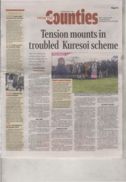


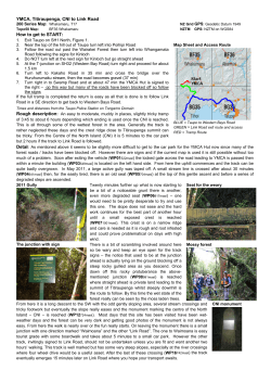


© Copyright 2026