Novelty Detection (One-Class Classification) Feb 2014 Dr. Lei Clifton How to use NDtool Overview The NDtool toolbox implements the several Novelty Detection (ND) methods, demonstrated in the demo function “demoND” whose input parameter NDtype specifies the data set and the ND method. After adding NDtool to your Matlab path, run the following example code: whichdata = 'banana_n200200s1'; NDtype = 'parzen'; demoND(whichdata, NDtype); Matlab will produce Figures 1-3. Line 60-72 of “demoND” shows the following ND methods for you to choose from (here we have chosen NDtype = 'parzen'): % NDtype = 'dist'; % a distance-based method (LC Thesis, Chapter 4.1) % NDtype = 'nn'; % a distance-based method (LC Thesis, Chapter 4.2) % NDtype = 'kmeans'; % a k-means method (LC Thesis, Chapter 4.3) NDtype = 'parzen'; % Parzen window method (LC Thesis, Chapter 3.3) % % % % NDtype = 'parzen'; % Parzen window method (LC Thesis, Chapter 3.3) NDtype = 'gmm'; % Gaussian mixture model method NDtype = 'svmTax'; % one-class SVM by Tax, 2001 (Type I in LC Thesis) NDtype = 'svmSch'; % one-class SVM by Scholkopf, 2000 (Type II in LC Thesis) % % % % % NDtype = 'gpoc'; NDtype = 'kde'; NDtype = 'som'; NDtype = 'pca'; NDtype = 'kpca'; % one-class Gaussian process method % Kernel density estimator % self organising map method using Netlab toolbox. % principal component analysis method % kernel PCA method Procedure for performing a ND task Step 1: load a data set. There is a sub-folder called “data” in folder “NDtool”. This “data” folder stores some example data sets. In the above example code, we have loaded data set “banana_n200200s1. The demo function “demoND” loads the data set (data.x) and their class labels (data.y) at Line 103106, and then separates normal data from abnormal data at Line 126-129. The code segment is as follows: data = load(whichdata); fprintf('\nLoading data set %s...\n', whichdata); alldataOri = data.x; % numdata by numftrs classlabels = data.y; % numdata by 1, class labels = 1, 2 isnor = classlabels == 1; % regard class 1 as normal. isab = ~isnor; normaldataOri = alldataOri(isnor); Page 1 of 5 Novelty Detection (One-Class Classification) Feb 2014 Dr. 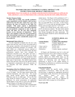Lei Clifton abnormaldataOri = alldataOri(~isnor); Figure 1: original data (left) and scaled data (right). Note that the scales of the two figures are different, but the scaled features have preserved the characteristics of the original features. Step 2: split and scale the data. After loading our data set, we will first split the data into three groups: training, validation, and test data using function “splitData”, and then scale all the data using “scaleData”. The features are plotted in “runND”, Line 253-297. Split the data Function “splitData” splits data into three groups: training data, test data, and validation data. Note that its second input “isab” is a logical vector containing values “true” or “false”, indicating which part of its first input “alldata” contains abnormal data. The following code segment shows you how to set the two inputs correctly (code is from Line 105-106, 126-127, 140 of the demo function “demoND”): alldataOri = data.x; % numdata by numftrs classlabels = data.y; % numdata by 1, class labels = 1, 2 isnor = classlabels == 1; % regard class 1 as normal. isab = ~isnor; [traindataNorOri, testdataNorOri, validdataNorOri, validdataAbOri, testdataAbOri] = splitData(alldataOri, isab); Scale the data Scaling the data is also called normalising the data. You have previously learned how to normalise data using the zero-mean, unit-variance transformation shown below, xf’ = (xf – μf) / σf, Page 2 of 5 Feb 2014 Novelty Detection (One-Class Classification) Dr. Lei Clifton where μf and σf are the mean and standard deviation, respectively, of feature f . Which group of data should you use to derive μf and σf ? Why? This is an important question to ask yourself before you start any novelty detection task. (Answer: normal training data) Step 3: Train a machine. We have prepared our data in steps 1 and 2 above; now we will choose a Novelty Detection method, and then train a machine using the training data. For example, if we have chosen the Parzen window method (NDtype = 'parzen'), the training will be performed by function “train_parzen”. Step 4: Use the trained machine to calculate novelty scores of any give data. We have trained a Parzen window machine in Step 3 above, now we will use it to calculate novelty scores. This is done by function “out_parzen”. The resulting novelty scores are shown in Figure 2, and a contour plot is shown in Figure 3. Note: Function “out_parzen” calls a sub-function “kernelGau” at Line 32. 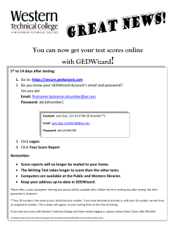Figure 2: Novelty scores (shown on y-axis) obtained using training normal data, test normal data, and test abnormal data. The optimal threshold set by the validation data is shown in a black dash-and-dotted line. Page 3 of 5 Feb 2014 Novelty Detection (One-Class Classification) Dr. Lei Clifton Step 5: Use the validation data to set a threshold for the chosen novelty detection method, if applicable We have obtained the novelty scores of our data in Step 4 above. How do we decide whether the given data are normal or abnormal, based on these novelty scores? Some novelty detection methods (e.g., SVMs type I and type II) have already specified their thresholds, while others (e.g., Parzen window, GMM) require us to specify a threshold for them. Let’s continue the Parzen window method in Step 4: the usual approach is to use the validation data to set a threshold on the novelty scores (recall that we have split the data into three groups in Step 2). A data point is deemed “abnormal” if its novelty score exceeds the threshold. Now we will use the validation data to set a threshold for the chosen novelty detection method, using function “minErr_thr”. Note that the validation process usually requires the existence of both normal and abnormal data. The resulting threshold is shown in a black dash-and-dotted line in Figure 2. In function “runND”, Line 183-198 shows how to set threshold for different ND methods. Step 6: Assign class labels for the given data Finally we assign class labels for the given data, depending on whether or not their novel scores are above the threshold obtained in Step 5. 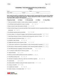This is the final step of a novelty detection task, performed by function “assignCls”. Figure 3 shows a contour plot of the novelty scores over the 2D feature space of the chosen data set “banana_n200200s1”. Note that the optimal threshold using the validation data is 0.037 for this data set, which is somewhere between the two black contour lines shown in Figure 3. Page 4 of 5 Feb 2014 Novelty Detection (One-Class Classification) Dr. Lei Clifton Figure 3: Contour plot of novelty scores obtained using Parzen window method, over a 2D feature space. Normal and abnormal data are shown in white and black colour, respectively. Normal training data, normal test data, and abnormal data are shown in {x, +, ·}, respectivelty. Note that the optimal threshold using the validation data is 0.037 for this data set, which is somewhere between the two black contour lines shown in this figure. Summary Congratulations – you have learned all steps for performing a novelty detection method. Now here is some questions for you: Q1: What is the code structure for any chosen novelty detection method? For example, if you have set NDtype = ‘svmSch’ in the code above, what functions will be called in demoND? Q2: Choose a different data set and different novelty detection method, and produce your results. How many features and classes does your data set have? What data are regarded as normal and abnormal? How do you understand your results? Q3: What is a confusion matrix, and how do you compute it? Hint: Function “runND” calls a Netlab function “confmat” at Line 212. Q4: How does function “demoND” add necessary paths? How would you do this yourself if you need to use this toolbox for you own application? Hint: Go to Line 89. Q5: What are the meanings of the outputs of function “demoND”? How would you use them for your own application? Page 5 of 5