1. No category

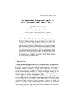
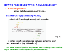
Molecular Systems Biology 3; Article number 78; doi:10.1038/msb4100120
Citation: Molecular Systems Biology 3:78
& 2007 EMBO and Nature Publishing Group All rights reserved 1744-4292/07
www.molecularsystemsbiology.com
REVIEW
How to infer gene networks from expression profiles
Mukesh Bansal1,2,5, Vincenzo Belcastro3,5,
Alberto Ambesi-Impiombato1,4 and Diego di Bernardo1,2,*
1
Telethon Institute of Genetics and Medicine, Via P Castellino, Naples, Italy,
European School of Molecular Medicine, Naples, Italy,
3
Department of Natural Sciences, University of Naples ‘Federico II’, Naples,
Italy and
4
Department of Neuroscience, University of Naples ‘Federico II’, Naples, Italy
5
These authors contributed equally to this work
* Corresponding author. Systems Biology Lab, Telethon Institute of Genetics
and Medicine, Via P Castellino 111, Naples 18131, Italy.
Tel.: þ 39 081 6132 319; Fax: þ 39 081 6132 351;
E-mail: [email protected]
2
Received 30.5.06; accepted 18.12.06
Inferring, or ‘reverse-engineering’, gene networks can
be defined as the process of identifying gene interactions
from experimental data through computational analysis.
Gene expression data from microarrays are typically used
for this purpose. Here we compared different reverseengineering algorithms for which ready-to-use software
was available and that had been tested on experimental
data sets. We show that reverse-engineering algorithms
are indeed able to correctly infer regulatory interactions
among genes, at least when one performs perturbation
experiments complying with the algorithm requirements.
These algorithms are superior to classic clustering algorithms for the purpose of finding regulatory interactions
among genes, and, although further improvements are
needed, have reached a discreet performance for being
practically useful.
Molecular Systems Biology 13 February 2007;
doi:10.1038/msb4100120
Subject Categories: metabolic and regulatory networks; simulation
and data analysis
Keywords: gene network; reverse-engineering; gene expression;
transcriptional regulation; gene regulation
Introduction
Gene expression microarrays yield quantitative and semiquantitative data on the cell status in a specific condition and
time. Molecular biology is rapidly evolving into a quantitative
science, and as such, it is increasingly relying on engineering
and physics to make sense of high-throughput data. The aim is
to infer, or ‘reverse-engineer’, from gene expression data, the
regulatory interactions among genes using computational
algorithms. There are two broad classes of reverse-engineering
algorithms (Faith and Gardner, 2005): those based on the
‘physical interaction’ approach that aim at identifying interactions among transcription factors and their target genes
& 2007 EMBO and Nature Publishing Group
(gene-to-sequence interaction) and those based on the
‘influence interaction’ approach that try to relate the expression of a gene to the expression of the other genes in the cell
(gene-to-gene interaction), rather than relating it to sequence
motifs found in its promoter (gene-to-sequence). We will refer
to the ensemble of these ‘influence interactions’ as gene
networks.
The interaction between two genes in a gene network does
not necessarily imply a physical interaction, but can also refer
to an indirect regulation via proteins, metabolites and ncRNA
that have not been measured directly. Influence interactions
include physical interactions, if the two interacting partners
are a transcription factor, and its target, or two proteins in the
same complex. Generally, however, the meaning of influence
interactions is not well defined and depends on the mathematical formalism used to model the network. Nonetheless,
influence networks do have practical utility for (1) identifying
functional modules, that is, identify the subset of genes that
regulate each other with multiple (indirect) interactions, but
have few regulations to other genes outside the subset;
(2) predicting the behaviour of the system following perturbations, that is, gene network models can be used to predict
the response of a network to an external perturbation and
to identify the genes directly ‘hit’ by the perturbation (di
Bernardo et al, 2005), a situation often encountered in the drug
discovery process, where one needs to identify the genes that
are directly interacting with a compound of interest; (3)
identifying real physical interactions by integrating the gene
network with additional information from sequence data and
other experimental data (i.e. chromatin immunoprecipitation,
yeast two-hybrid assay, etc.).
In addition to reverse-engineering algorithms, network
visualisation tools are available online to display the network
surrounding a gene of interest by extracting information from
the literature and experimental data sets, such as Cytoscape
(Shannon et al, 2003) (http://www.cytoscape.org/features.php)
and Osprey (Breitkreutz et al, 2003) (http://biodata.mshri.on.
ca/osprey/servlet/Index).
Here we will focus on gene network inference algorithms
(the influence approach). A description of other methods
based on the physical approach and more details on
computational aspects can be found in (Beer and Tavazoie,
2004; Tadesse et al, 2004; Faith and Gardner, 2005; Prakash
and Tompa, 2005; Ambesi and di Bernardo, 2006; Foat et al,
2006). We will also briefly describe two ‘improper’ reverseengineering tools (MNI and TSNI), whose main focus is not
inferring interactions among genes from gene expression data,
but rather identification of the targets of the perturbation
(point (2) above).
Among the plethora of algorithms proposed in the literature
to solve the network inference problem, we selected one
algorithm for each class of mathematical formalism proposed
in the literature, for which ready-to-use software is available
and that had been tested on experimental data sets.
Molecular Systems Biology 2007 1
How to infer gene networks from expression profiles
M Bansal et al
understand what can be gained by advanced gene network
inference algorithms, whose aim is to infer direct interactions
among genes, as compared with ‘simple’ clustering, for the
purpose of gene network inference.
The most common clustering approach is hierarchical
clustering (Eisen et al, 1998), where relationships among
genes are represented by a tree whose branch lengths reflect
the degree of similarity between genes, as assessed by a
pairwise similarity function such as Pearson correlation
coefficient:
Gene network inference algorithms
We will indicate the gene expression measurement of gene i
with the variable xi, the set of expression measurements for all
the genes with D and the interaction between genes i and j
with aij. D may consist of time-series gene expression data of
N genes in M time points (i.e. gene expression changing
dynamically with time), or measurements taken at steadystate in M different conditions (i.e. gene expression levels in
homeostasis). Some inference algorithms can work on both
kind of data, whereas others have been specifically designed
to analyse one or the other.
Depending on the inference algorithm used, the resulting
gene network can be either an undirected graph, that is, the
direction of the interaction is not specified (aij¼aji), or a
directed graph specifying the direction of the interaction, that
is, gene j regulates gene i (and not vice versa) (aijaaji). A
directed graph can also be labeled with a sign and strength
for each interaction, signed directed graph, where aij has a
positive, zero or negative value indicating activation, no
interaction and repression, respectively.
An overview of softwares described here is given in Figure 1
and Table I.
M
P
ðxi ðkÞxj ðkÞÞ
ffiffiffiffiffiffiffiffiffiffiffiffiffiffiffiffiffiffiffiffiffiffiffiffiffiffiffiffiffiffiffiffiffiffiffiffiffi
rij ¼ sffiffiffik¼1
M
M
P
P
ð x2i ðkÞ
x2j ðkÞÞ
k¼1
Clustering, although not properly a network inference algorithm, is the current method of choice to visualise and analyse
gene expression data. Clustering is based on the idea of
grouping genes with similar expression profiles in clusters
(Eisen et al, 1998). Similarity is measured by a distance metric,
as for example the correlation coefficient among a pair of
genes. The number of clusters can be set either automatically
or by the user depending on the clustering algorithm used
(Eisen et al, 1998; Amato et al, 2006). The rationale behind
clustering is that coexpressed genes (i.e. genes in the same
cluster) have a good probability of being functionally related
(Eisen et al, 1998). This does not imply, however, that there is a
direct interaction among the coexpressed genes, as genes
separated by one or more intermediaries (indirect relationships) may be highly coexpressed. It is therefore important to
Infer a gene network?
Bayesian networks
A Bayesian network is a graphical model for probabilistic
relationships among a set of random variables Xi, where
i¼1 y n. These relationships are encoded in the structure of
a directed acyclic graph G, whose vertices (or nodes) are the
random variables Xi. The relationships between the variables
No
Predict targets of a
perturbation?
Yes
ARACNE(*)
BANJO (DBN)
CLUSTERING
Time
series
What kind of
expression
data?
Steady state
ARACNE
BANJO (BN)
NIR
CLUSTERING
k¼1
For a set of n profiles, all the pairwise correlation coefficients
rij are computed; the highest value (representing the most
similar pair of genes) is selected and a node in the tree is
created for this gene pair with a new expression profile given
by the average of the two profiles. The process is repeated by
replacing the two genes with a single node, and all pairwise
correlations among the n%1 profiles (i.e. n%2 profiles from
single genes plus 1 of the gene pair) are computed. The process
stops when only one element remains. Clusters are obtained
by cutting the tree at a specified branch level.
In order to compare clustering to the other network
inference strategies, we assumed that genes in the same
clusters regulate each other, that is, each gene represents a
node in the network and is connected to all the other genes in
the same cluster. Clustering will thus recover an undirected
graph.
Coexpression networks and clustering algorithms
START
(Expression data)
ð1Þ
Yes
What kind of
expression
data?
Time
series
TSNI
Steady state
MNI
NIR
Figure 1 Flowchart to choose the most suitable network inference algorithms according to the problem to be addressed. (*): check for independence of time points
(see text for details); (BN): Bayesian networks; (DBN): Dynamic Bayesian Networks.
2 Molecular Systems Biology 2007
& 2007 EMBO and Nature Publishing Group
How to infer gene networks from expression profiles
M Bansal et al
Table I Features of the network inference algorithms reviewed in this tutorial
Software
Download
Data
type
Command line
Notes
BANJO
www.cs.duke.edu/~amink/
software/banjo
S/D
java-jar banjo.jar settingFile¼mysettings.txt
Good performance if large datasets
is available (MbN)
ARACNE
amdec-bioinfo.cu-genome.org/html/
caWork-Bench/upload/arcane.zip
S/D
arance-i inputfile-o
outputfile [options]
Good performance even for MpN. Not useful
for short time series
NIR/MNIa
[email protected]
S
MATLAB
NIR: good performance but requires knowledge
of perturbed genes/MNI: good performance for
inferring targets of a perturbation
Hierarchical
clustering
http://bonsai.ims.u-tokyo.ac.jp/
mde-hoon/software/cluster
S/D
GUI
Useful for finding coexpressed genes,
but not for network inference
Abbreviations: D: dynamic time-series; N: number of genes; M: number of experiments; S: steay-state.
a
Predicts only targets of a perturbation (see text for details).
Information-theoretic
Bayesian Networks
E
D
B
H
B
C
G
P(A/B,C,D,E)=P(A/B,C)
B
C
F
H
G
MI(A,H)=0
MI(A,B)>0
0 < MI(A,D)≤min{MI(A,B), MI(B,D)}
E
D
E
A
H
A
F
D
Ordinary differential equations
C
A
F
G
dA/dt=θ1A+θ2B+θ3C
or more generally:
dA/dt=f(A,B,C,θ)
Figure 2 Bayesian networks: A is conditionally independent of D and E given B and C; information-theoretic networks: mutual information is 0 for statistically
independent variables, and Data Processing Inequality helps pruning the network; ordinary differential equations: deterministic approach, where the rate of transcription
of gene A is a function (f) of the level of its direct causal regulators.
are described by a joint probability distribution P(X1, y, Xn)
that is consistent with the independence assertions embedded
in the graph G and has the form:
PðX1 ; . . . ; Xn Þ ¼
N
Y
i¼1
PðXi ¼ xi jjXj ¼ xj ; . . . ; Xjþp ¼ xjþp Þ
ð2Þ
where the p þ 1 genes, on which the probability is conditioned,
are called the parents of gene i and represent its regulators,
and the joint probability density is expressed as a product
of conditional probabilities by applying the chain rule of
probabilities and independence. This rule is based on the
Bayes theorem: PðA; BÞ ¼ PðBjjAÞ & PðAÞ ¼ PðAjjBÞ & PðBÞ:
We observe that the JPD (joint probability distribution) can
be decomposed as the product of conditional probabilities as
in Equation 2 only if the Markov assumption holds, that is,
each variable Xi is independent of its non-descendants, given
its parent in the directed acyclic graph G. A schematic
overview of the theory underlying Bayesian networks is given
in Figure 2.
& 2007 EMBO and Nature Publishing Group
In order to reverse-engineer a Bayesian network model
of a gene network, we must find the directed acyclic graph
G (i.e. the regulators of each transcript) that best describes
the gene expression data D, where D is assumed to be a
steady-state data set. This is performed by choosing a
scoring function that evaluates each graph G (i.e. a possible
network topology) with respect to the gene expression
data D, and then searching for the graph G that maximises
the score.
The score can be defined using the Bayes rule:
PðG=DÞ ¼ PðD=GÞ&PðGÞ
, where P(G) can either contain some a
PðDÞ
priori knowledge on network structure, if available, or can be a
constant non-informative prior, and P(D/G) is a function, to be
chosen by the algorithm that evaluates the probability that
the data D has been generated by the the graph G. The most
popular scores are the Bayesian Information Criteria (BIC) or
Bayesian Dirichlet equivalence (BDe). Both scores incorporate
a penalty for complexity to guard against overfitting of data.
Trying out all possible combinations of interaction among
genes, that is, all possible graphs G, and choosing the G with
Molecular Systems Biology 2007 3
How to infer gene networks from expression profiles
M Bansal et al
the maximum Bayesian score is an NP-hard problem. Therefore, a heuristic search method is used, like the greedy-hill
climbing approach, the Markov Chain Monte Carlo method
or simulated annealing.
In Bayesian networks, the learning problem is usually
underdetermined and several high-scoring networks are
found. To address this problem, one can use model averaging
or bootstrapping to select the most probable regulatory
interactions and to obtain confidence estimates for the
interactions. For example, if a particular interaction between
two transcripts repeatedly occurs in high-scoring models, one
gains confidence that this edge is a true dependency.
Alternatively, one can augment an incomplete data set with
prior information to help select the most likely model
structure. Bayesian networks cannot contain cycles(i.e. no
feedback loops). This restriction is the principal limitation of
the Bayesian network models. Dynamic Bayesian networks
overcome this limitation. Dynamic Bayesian networks are an
extension of Bayesian networks able to infer interactions from
a data set D consisting of time-series rather than steady-state
data. We refer the reader to (Yu et al, 2004).
A word of caution: Bayesian networks model probabilistic
dependencies among variables and not causality, that is, the
parents of a node are not necessarily also the direct causes of
its behaviour. However, we can interpret the edge as a causal
link if we assume that the Causal Markov Condition holds. This
can be stated simply as: a variable X is independent of every
other variable (except the targets of X) conditional on all its
direct causes. It is not known whether this assumption is a
good approximation of what happens in real biological
networks.
For more information and a detailed study of Bayesian
networks for gene network inference, we refer the reader
to Pe’er et al (2000).
Banjo
Banjo is a gene network inference software that has been
developed by the group of Hartemink (Yu et al, 2004). Banjo is
based on Bayesian networks formalism and implements both
Bayesian and Dynamic Bayesian networks. Therefore it can
infer gene networks from steady-state gene expression data
or from time-series gene expression data.
In Banjo, heuristic approaches are used to search the
‘network space’ to find the network graph G (Proposer/
Searcher module in Banjo). For each network structure
explored, the parameters of the conditional probability density
distribution are inferred and an overall network’s score is
computed using the BDe metric in Banjo’s Evaluator module.
The output network will be the one with the best score
(Banjo’s Decider module).
Banjo outputs a signed directed graph indicating regulation
among genes. Banjo can analyse both steady-state and timeseries data. In the case of steady-state data, Banjo, as well as
the other Bayesian networks algorithms, is not able to infer
networks involving cycles (e.g. feedback or feed forward
loops).
Other Bayesian network inference algorithms for which
software is available have been proposed (Murphy, 2001;
Friedman and Elidan, 2004).
4 Molecular Systems Biology 2007
Information-theoretic approaches
Information-theoretic approaches use a generalisation of
pairwise correlation coefficient in equation (1), called Mutual
Information (MI), to compare expression profiles from a set of
microarrays. For each pair of genes, their MIij is computed and
the edge aij¼aji is set to 0 or 1 depending on a significance
threshold to which MIij is compared. MI can be used to
measure the degree of independence between two genes.
Mutual information, MIij, between gene i and gene j is
computed as:
MIi;j ¼ Hi þ Hj % Hij
where H, the entropy, is defined as:
n
X
pðxk Þ logðpðxk ÞÞ
Hi ¼ %
k¼1
ð3Þ
ð4Þ
The entropy Hi has many interesting properties; specifically,
it reaches a maximum for uniformly distributed variables,
that is, the higher the entropy, the more randomly distributed
are gene expression levels across the experiments. From the
definition, it follows that MI becomes zero if the two variables
xi and xj are statistically independent (P(xixj)¼P(xi)P(xj)), as
their joint entropy Hij¼Hi þ Hj. A higher MI indicates that the
two genes are non-randomly associated to each other. It can
be easily shown that MI is symmetric, Mij¼Mji, therefore the
network is described by an undirected graph G, thus differing
from Bayesian networks (directed acyclic graph).
MI is more general than the Pearson correlation coefficient.
This quantifies only linear dependencies between variables,
and a vanishing Pearson correlation does not imply that two
variables are statistically independent. In practical application,
however, MI and Pearson correlation may yield almost
identical results (Steuer et al, 2002).
The definition of MI in equation (3) requires each data point,
that is, each experiment, to be statistically independent
from the others. Thus information-theoretic approaches, as
described here, can deal with steady-state gene expression
data set, or with time-series data as long as the sampling time
is long enough to assume that each point is independent of the
previous points.
Edges in networks derived by information-theoretic approaches represent statistical dependences among geneexpression profiles. As in the case of Bayesian network, the
edge does not represent a direct causal interaction between
two genes, but only a statistical dependency. A ‘leap of faith’
must be performed in order to interpret the edge as a direct
causal interaction.
It is possible to derive the information-theoretic approach as
a method to approximate the JPD of gene expression profiles,
as it is performed for Bayesian networks. We refer the
interested readers to Margolin et al (2006).
ARACNE
ARACNE (Basso et al, 2005; Margolin et al, 2006) belongs to
the family of information-theoretic approaches to gene
network inference first proposed by Butte and Kohane (2000)
with their relevance network algorithm.
ARACNE computes Mij for all pairs of genes i and j in the
data set. Mij is estimated using the method of Gaussian kernel
& 2007 EMBO and Nature Publishing Group
How to infer gene networks from expression profiles
M Bansal et al
density (Steuer et al, 2002). Once Mij for all gene pairs has been
computed, ARACNE excludes all the pairs for which the null
hypothesis of mutually independent genes cannot be ruled out
(Ho: MIij¼0). A P-value for the null hypothesis, computed
using Montecarlo simulations, is associated to each value of
the mutual information. The final step of this algorithm is a
pruning step that tries to reduce the number of false-positive
(i.e. inferred interactions among two genes that are not direct
causal interaction in the real biological pathway). They use the
Data Processing Inequality (DPI) principle that asserts that
if both (i,j) and (j,k) are directly interacting, and (i,k) is
indirectly interacting through j, then Mi, kpmin(Mij, Mjk). This
condition is necessary but not sufficient, that is, the inequality
can be satisfied even if (i, k) are directly interacting. Therefore
the authors acknowledge that by applying this pruning
step using DPI they may be discarding some direct interactions
as well.
Ordinary differential equations
Reverse-engineering algorithms based on ordinary differential
equations (ODEs) relate changes in gene transcript concentration to each other and to an external perturbation. By external
perturbation, we mean an experimental treatment that can
alter the transcription rate of the genes in the cell. An example
of perturbation is the treatment with a chemical compound
(i.e. a drug), or a genetic perturbation involving overexpression or downregulation of particular genes.
This is a deterministic approach not based on the estimation
of conditional probabilities, unlike Bayesian networks and
information-theoretic approaches. A set of ODEs, one for each
gene, describes gene regulation as a function of other genes:
.
xi ðtÞ ¼ fi ðx1 ; . . . ; xN ; u; yi Þ
ð5Þ
where yi is a set of parameters describing interactions among
genes (the edges of the graph), i¼1 y N, xi(t) is the
.
i
concentration of transcript i measured at time t, xi ðtÞ ¼ dx
dt ðtÞ
is the rate of transcription of transcript i, N is the number of
genes and u is an external perturbation to the system.
As ODEs are deterministic, the interactions among genes (yi)
represent causal interactions, and not statistical dependencies
as the other methods.
To reverse-engineer a network using ODEs means to choose
a functional form for fi and then to estimate the unknown
parameters yi for each i from the gene expression data D using
some optimisation technique.
The ODE-based approaches yield signed directed graphs and
can be applied to both steady-state and time-series expression
profiles. Another advantage of ODE approaches is that once
the parameters yi, for all i are known, equation (5) can be used
to predict the behaviour of the network in different conditions
(i.e. gene knockout, treatment with an external agent, etc.).
NIR, MNI and TSNI
In recent studies (Gardner et al, 2003; di Bernardo et al, 2005;
Bansal et al, 2006), ODE-based algorithms have been developed (Network identification by multiple regression (NIR) and
microarray network identifcation (MNI)) that use a series of
steady-state RNA expression measurements, or time-series
& 2007 EMBO and Nature Publishing Group
measurements (time-series network identification—TSNI)
following transcriptional perturbations, to reconstruct gene–
gene interactions and to identify the mediators of the activity
of a drug. Other algorithms based on ODEs have been
proposed in the literature (D’haeseleer et al, 1999; Tegner
et al, 2003; Bonneau et al, 2006; van Someren et al, 2006).
The network is described as a system of linear ODEs (de
Jong, 2002) representing the rate of synthesis of a transcript
as a function of the concentrations of every other transcript
in a cell, and the external perturbation:
N
X
.
xi ðtk Þ ¼
aij xj ðtk Þ þ bi uðtk Þ
j¼1
ð6Þ
where i¼1 ,y, N; k¼1 y M, N is the number of genes, M is the
.
number of time points, xi(tk) is the concentration of transcript i
.
measured at time tk, xi(tk) is the rate of change of concentration
of gene i at time tk, that is, the first derivative of the mRNA
concentration of gene i measured at time tk, aij represents the
influence of gene j on gene i, bi represents the effect of the
external pertrurbation on xi and u(tk) represents the external
perturbation at time tk (aij and bi are the y in equation (5)).
.
In the case of steady-state data, xi(tk)¼0 and equation (6) for
gene i becomes independent of time and can be simplified and
rewritten in the form of a linear regression:
N
X
j¼1
aij xj ¼ %bi u
ð7Þ
The NIR algorithm (Gardner et al, 2003) computes the edges aij
from steady-state gene expression data using equation (7). NIR
needs, as input, the gene expression profiles following each
perturbation experiment (xj), knowledge of which genes have
been directly perturbed in each perturbation experiment (biu)
and optionally, the standard deviation of replicate measurements. NIR is based on a network sparsity assumption, that is,
a maximum number of ingoing edges per gene (i.e. maximum
number of regulators per gene), which can be chosen by the
user. The output is in matrix format, where each element is the
edge aij. The inference algorithm reduces to solving equation
(7) for the unknown parameters aij, that is, a classic linearregression problem.
The MNI algorithm (di Bernardo et al, 2005) is based on
equation (7) as well, and uses steady-state data like NIR, but
importantly, each microarray experiment can result from any
kind of perturbation, that is, we do not require knowledge
of biu. MNI is different from other inference methods as the
inferred network is used not per se but to filter the gene
expression profile following a treatment with a compound
to determine pathways and genes directly targeted by the
compound. This is achieved in two steps. In the first step, the
parameters aij are obtained from gene expression data D;
in the second step, the gene expression profile following
compound treatment is measured (xdi with i¼1 y N), and
equation (7) is used to compute the values biu for each i, as
aij is known and u is simply a constant representing the
treatment. bi different from 0 represents the genes that are
directly hit by the compound. The output is a ranked list of
genes; genes at the top of the list are the most likely targets of
the compound (i.e. the ones with the highest value of bi).
Molecular Systems Biology 2007 5
How to infer gene networks from expression profiles
M Bansal et al
The network inferred by MNI could be used per se, and not
only as a filter; however, if we do not have any knowledge
about which genes have been perturbed directly in each
perturbation experiment in dataset D (right-hand side in
equation (7)), then, differently from NIR, the solution to
equation (7) is not unique, and we can only infer one out of
many possible networks that can explain the data. What
remains unique are the predictions (bi), that is, all the possible
networks predict the same bi.
MNI performance is not tested here, not being a ‘proper’
network inference algorithm, but we refer the interested
readers to di Bernardo et al (2005), where the performance
is tested in detail.
The TSNI (Time Series Network Identification) algorithm
(Bansal et al, 2006) identifies the gene network (aij) as well as
the direct targets of the perturbations (bi). TSNI is based on
equation (6) and is applied when gene expression data are
dynamic (time-series). To solve equation (6), we need the values
.
of xi(tk) for each gene i and each time point k. This can be
estimated directly from the time-series of gene expression
profiles. TSNI assumes that a single perturbation experiment is
performed (e.g. treatment with a compound, gene overexpression, etc.) and M time points following the perturbation are
measured (rather than M different conditions at steady-state as
for NIR and MNI). For small networks (tens of genes), it is able to
correctly infer the network structure (i.e. aij). For large networks
(hundreds of genes), its performance is best for predicting the
direct targets of a perturbation (i.e. bi) (for example, finding the
direct targets of a transcription factor from gene expression time
series following overexpression of the factor). TSNI is not tested
here, but we refer the reader to Bansal et al (2006).
Reverse-engineering algorithm
performance
We performed a comparison using ‘fake’ gene expression data
generated by a computer model of gene regulation (‘in silico’
data). The need of simulated data arises from imperfect
knowledge of real networks in cells, from the lack of suitable
gene expression data set and of control on the noise levels.
In silico data enable one to check the performance of
algorithms against a perfectly known ground truth (simulated
networks in the computer model).
To simulate gene expression data and gene regulation in the
form of a network, we use linear ODEs relating the changes in
gene transcript concentration to each other and to the external
perturbations. Linear ODEs can simulate gene networks as
directed signed graphs with realistic dynamics and generate both
steady-state and time-series gene expression profiles. Linear
ODEs are generic, as any non-linear process can be approximated to a linear process, as long as the system is not far from
equilibrium, whereas non-linear processes are all different from
each other. There are many other choices possible (Brazhnik
et al, 2003), but we valued the capability of linear ODEs of
quickly generating many random networks with realistic
behaviour and the availability of a general mathematical theory.
We generated 20 random networks with 10, 100 and 1000
genes and with an average in-degree per gene of 2, 10 and 100,
respectively. For each network we generated three kinds of
6 Molecular Systems Biology 2007
data: steady-state-simulated microarray data resulting from M
global perturbations (i.e. all the genes in the network are
perturbed simultaneously in each perturbation experiment);
steady-state data resulting from M local perturbations (i.e.
a different single gene in the network is perturbed in each
experiment) and dynamic time-series-simulated microarray
data resulting from perturbing 10% of the genes simultaneously and measuring M time points following the perturbation experiment. For all data sets, M was chosen equal to 10,
100 and 1000 experiments. Noise was then added to all data
sets by summing to each simulated gene expression level in the
data set, white noise with zero mean and standard deviation
equal to 0.1 multiplied by the absolute value of the simulated
gene expression level (Gardner et al, 2003).
All the algorithms were run on all the data sets using default
parameters (Supplementary Table 1). Banjo was not run on the
1000 gene data set, as it was crashing owing to memory
limitations, whereas NIR needed an excessively long computation time.
Results from the simulations are described in Table II. PPV
stands for positive predictive value (or accuracy) defined as
TP/(TP þ FP) and Sensitivity (Se) is TP/(TP þ FN), where TP,
true positive; FP, false positive and FN, false negative. The label
‘Random’ refers to the expected performance of an algorithm
that selects a pair of genes randomly and ‘infers’ an edge
between them. For example, for a fully connected network,
the random algorithm would have a 100% accuracy for all the
levels of sensitivity (as any pair of genes is connected in the
real network). Some algorithms infer the network just as
an undirected graph, and others as a directed and/or signed
graph. Thus, in order to facilitate comparison among
algorithms, we computed PPV and Se by first transforming
the real (signed directed graph) and the inferred networks
(when directed and/or signed) in an undirected graph (labeled
u
in the table). If the algorithm infers a directed graph and/or
a signed directed graph, we also compared PPV and Se in
this case (labeled d and s, respectively, in the table). When
computing PPV and Se we did not include self-feedback
loops (diagonal elements of the adjacency matrix), as all the
simulated networks have self-feedback loops, and this could
be an advantage for some algorithms as NIR that always
recovers a network with self-feedbacks.
We observe that for the ‘global’ perturbation data set, all the
algorithms, but Banjo, (Bayesian networks) fail, as their
performance is comparable with the random algorithm (hence
the importance of reporting always the random performance).
Banjo performance is poor when only 10 experiments are
available, and reaches a very good accuracy for 100 experiments (independently of the number of genes), albeit with
a very low sensitivity (only few edges are found). The
performance of all the algorithms, but Banjo, improves
dramatically for the ‘local’ data set. In this case, both ARACNE
and NIR perform very well, whereas Banjo performance is still
random for 10 experiments, whereas it reaches a very good
accuracy but poor sensitivity for the 100 experiments set.
Clustering is better than random, but is clearly not a good
method to infer gene networks. Performance is again random
for the time-series ‘dynamic’ data set. In this case we run
ARACNE as well, although the time points cannot be assumed
independent from each other. Banjo has been shown to work
& 2007 EMBO and Nature Publishing Group
How to infer gene networks from expression profiles
M Bansal et al
Table II Results of the application of network inference algorithms on the simulated data set
ARACNE
PPV
BANJO
NIR
Clustering
Random
Se
PPV
Se
PPV
Se
PPV
Se
PPV
Global (steady-state)
10 '10
0.37u
0.40u
0.41u
0.25d
0.16s
0.49u
0.17d
0.05s
0.34u
0.18d
0.09s
0.71u
0.45d
0.22s
0.40u
0.38u
0.36u
0.20d
0.10s
10 '100
0.37u
0.44u
0.96u
0.79d
0.84s
0.11u
0.05d
0.05s
0.36u
0.20d
0.09s
0.70u
0.46d
0.21s
0.36u
0.36u
0.36u
0.20d
0.10s
100 '10
0.19u
0.11u
0.19u
0.10d
0.06s
0.04u
0.02d
0.00s
0.18u
0.10d
0.05s
0.09u
0.05d
0.02s
0.19u
0.11u
0.19u
0.10d
0.05s
100 '100
0.19u
0.17u
0.70u
0.47d
0.71s
0.00u
0.00d
0.00s
0.19u
0.10d
0.05s
0.19u
0.10d
0.05s
0.19u
0.11u
0.19u
0.10d
0.05s
100 '1000
0.19u
0.26u
0.99u
0.68d
0.68s
0.05u
0.03d
0.03s
0.20u
0.10d
0.05s
0.19u
0.09d
0.05s
0.19u
0.11u
0.19u
0.10d
0.05s
1000 '1000
0.02u
0.10u
—
—
—
—
0.02u
0.01u
0.02u
0.53u
0.61u
0.41u
0.25d
0.15s
0.50u
0.18d
0.05s
0.63u
0.57d
0.57s
0.96u
0.93d
0.93s
0.39u
0.38u
0.36u
0.20d
0.10s
100 '100
0.56u
0.28u
0.71u
0.42d
0.60s
0.00u
0.00d
0.00s
0.97u
0.96d
0.96s
0.87u
0.86d
0.86s
0.29u
0.18u
0.19u
0.10d
0.05s
1000 '1000
0.66u
0.65u
—
—
—
—
0.20u
0.10u
0.02u
0.39u
0.36u
0.22d
0.00s
0.35u
0.21d
0.00s
—
—
0.35u
0.33u
0.36u
0.20d
0.10s
Local (steady-state)
10 '10
Dynamic (time-series)
10 '10
0
10 '100
0.35u
0.43u
0.36u
0.21d
0.25s
0.29u
0.16d
0.00s
—
—
0.35u
0.33u
0.36u
0.20d
0.10s
100 '10
0.19u
0.10u
0.18u
0.10d
0.06s
0.08u
0.04d
0.00s
—
—
0.19u
0.12u
0.19u
0.10d
0.05s
100 '100
0.19u
0.15u
0.19u
0.10d
0.04s
0.05u
0.02d
0.00s
—
—
0.19u
0.11u
0.19u
0.10d
0.05s
100 '1000
0.19u
0.19u
—
0.19u
0.11u
0.02u
0.10u
0.04u
0.02d
0.00s
—
—
1000 '1000
0.19u
0.10d
0.05s
—
—
—
0.02u
0.01u
0.19u
0.10d
0.05s
0.02u
Abbreviations: PPV: positive predicted value; Se: sensitivity.
In bold are the algorithms that perform significantly better than random, using as a random model a Binomial distribution.
on dynamic data, but needs a very high number of experiments
(time points) as compared with the number of genes (Yu et al,
2004).
In the ‘local’ data set, most of the algorithms perform better
than random: Banjo recovers only a few of the hundreds of real
interactions (low sensitivity and high accuracy), ARACNE
recovers about half of the real connections in the network
(good sensitivity and good accuracy), NIR instead recovers
& 2007 EMBO and Nature Publishing Group
almost all of the real interactions (high sensitivity and high
accuracy), clustering recovers a fifth of the real connections
but with low accuracy, and most of the connections recovered
by clustering are found by ARACNE as well.
It is interesting to ask what is the average overlap between
the inferred networks for the different algorithms. Supplementary Figure 1 shows an example of a 10-gene network
recovered by each of the four algorithms.
Molecular Systems Biology 2007 7
How to infer gene networks from expression profiles
M Bansal et al
We intersected the networks inferred by all the algorithms
and found that for the 10-gene network ‘local’ dataset,
on average about 10% of the edges overlap across all the
four algorithms, whereas about 0.01% overlap for the
100-gene network ‘local’ dataset (Supplementary Table 2).
This is due to the fact that Banjo for the 100-gene network
dataset recovers very few connections compared with the
other algorithms, thus the intersection has very few edges in
this case; excluding Banjo when computing the intersection
rescues the intersection overlap to about 10% (Supplementary
Table 2).
We then checked the PPV and Se by considering only the
edges that were found by all the algorithms, if any, as reported
in Supplementary Table 2. As expected, Se decreased, but the
PPV improved only slightly compared with that of each
algorithm considered separately. In addition, for large networks (100 genes), the intersection among the networks exists
only 35% of the time, whereas for small networks (10 genes),
it exists 95% of the time.
The performance of each algorithm can be further improved
by modifying their parameters (refer to Supplementary Table
3). The ARACNE parameter DPI (threshold for data processing
inequality) varies from 0 to 1 and controls the pruning of the
triplets in the network (1, no pruning and 0, each triplet is
broken at the weakest edge). We found a DPI¼0.15 to be
a conservative threshold giving a good compromise between
Se and PPV (Supplementary Table 3). Another parameter is
the threshold on the MI. Increasing these parameters allows
one to improve the PPV at the cost of reducing the Se. The MI
level can also be chosen automatically by ARACNE, which
does a fairly good job; so we suggest not to set the MI threshold
manually.
Banjo gives the user a variety of choices for its parameters:
the running time can be increased but it does not seem to affect
the results much (Supplementary Table 3); so we suggest 60 s
for 10-gene networks and 600 s for 100-gene networks; the
Proposer and Searcher modules, which scan and score the
network topology to find the best directed acyclic graph, can be
chosen from a set of four different algorithms; on our data sets,
the different choices did not affect the results considerably.
The NIR algorithm performance can be affected by varying
the parameter k, which defines the average in-degree per node
(i.e. each gene can be regulated at most by other k genes). The
lower the k, the higher the PPV at the cost of reducing the Se.
The performance of NIR on the simulated data sets is biased as
NIR is based on linear ODEs, which are also used to generate
the ‘fake’ simulated gene expression data; however, as noise is
added to the simulated data the reported performance should
not be too far from the true one. NIR seems to perform better
than the other algorithms, but it also requires more information, that is, the genes that have been directly perturbed in
each microarray experiment (for example, which gene has
been knocked-out, etc.).
Application to experimental data
In order to test different softwares, we also collected the
experimental data sets described in Table III and included in
the Supplementary material. The microarray data to be given
as input to the algorithms need no specific pre-processing, just
normalisation and selection of the genes that have responded
significantly to the perturbation experiments, using standard
techniques. We chose three different organisms and data sets
of different sizes: two large data sets (A and B), two medium
data sets (C and D) and two small data sets (E and F). We tested
each algorithm on the largest number of data sets possible. In
each case we used default parameters. Banjo could not run
on data set A and B owing to the large size of the dataset. NIR
can be applied only to dataset E, as it requires steady-state
experiments and knowledge of the perturbed gene in each
experiment. Hierarchical clustering was applied to all data
sets.
Table IV summarises the results but it should not be used
for comparative purposes between the different algorithms,
owing to the limited number of data and to the imperfect
knowledge of the real network. In silico analysis performed
in the previous section is better suited for this task.
ARACNE performs well on datasets A and C, whereas the
other algorithms are not significantly better than random.
ARACNE is not better than random for data set B and better
than random for dataset D, whereas Banjo is considerably
better than random for data set D, albeit with very low
sensitivity, in line with the in silico results. For the same
dataset, D, clustering performs better than random, with a
lower accuracy than Banjo, but a better sensitivity. The overall
low performance on dataset B, as compared with the other
data sets, is probably due either to higher noise levels in this
dataset or to imperfect knowledge of the real network
(transcription network in yeast).
Data sets E and F are not very informative since the real
networks are small and densely connected and therefore the
random algorithm performs very well. In any case, only NIR
performs significantly better than random for dataset E, and
only clustering does significantly better than random for
dataset F.
Table III Experimental data sets used as examples
ID
Cell/organism
Type
Samples
Genes
Reference
True network
A
B
C
D
E
F
HumanBcells
S. cerevisiae
HumanBcells
S. cerevisiae
E. coli
E. coli
S
S
S
S
S
T
254
300
254
300
9
6
7907
6312
23
90
9
9
(Basso et al, 2005)
(Hughes et al, 2000)
(Basso et al, 2005)
(Hughes et al, 2000)
(Gardner et al, 2003)
gardnerlab.bu.edu
Twenty-six Myc targets (Basso et al, 2005)
Eight hundred and forty-four TF–gene interactions (Lee et al, 2002)
11 Myc targets+11 non-targets (Basso et al, 2005)
Subset of TF–gene interactions (Lee et al, 2002)
Nine-gene network (Gardner et al, 2003)
Nine-gene network (Gardner et al, 2003)
Abbreviations: S: steady-state; T: time-series.
8 Molecular Systems Biology 2007
& 2007 EMBO and Nature Publishing Group
How to infer gene networks from expression profiles
M Bansal et al
Table IV Results of the application of network inference algorithms on the experiment data sets
Data sets
ARACNE
PPV
BANJO
Se
PPV
A
B
C
D
E
u
u
0.14
0.00u
0.78u
0.07u
0.69u
0.35
0.01u
0.64u
0.17u
0.34u
F
0.75u
0.37u
—
—
0.60u
0.17u
0.78u
0.67d
0.50s
0.73u
0.61d
0.00s
NIR
Se
—
—
0.27u
0.02u
0.44u
0.24d
0.02s
0.69u
0.39d
0.00s
PPV
—
—
—
—
0.80u
0.74d
0.59s
—
Clustering
Se
—
—
—
—
0.88u
0.67d
0.53s
—
PPV
Random
se
PPV
u
u
0.02
0.00u
0.45u
0.11u
0.8u
1.00
0.21u
0.91u
0.44u
0.63u
0.90u
0.59u
0.00u
0.00u
0.48u
0.04u
0.71u
0.63d
0.32s
0.71u
0.63d
0.32s
Abbreviations: PPV: positive predicted value; Se: sensitivity.
In bold are the algorithms that perform significantly better than random (P-valuep0.1) using as a random model a Binomial distribution.
Discussion and conclusions
In silico analysis gives reliable guidelines on algorithms’
performance in line with the results obtained on real data sets:
ARACNE performs well for steady-state data and can be
applied also when few experiments are available, as compared
with the number of genes, but it is not suited for the analysis
of short time-series data. This is to be expected owing to the
requirement of statistically independent experiments. Banjo is
very accurate, but with a very low sensitivity, on steady-state
data when more than 100 different perturbation experiments
are available, independently of the number of genes, whereas
it fails for time-series data. Banjo (and Bayesian networks in
general) is a probabilistic algorithm requiring the estimation
of probability density distributions, a task that requires large
number of data points. NIR works very well for steady-state
data, also when few experiments are available, but requires
knowledge on the genes that have been perturbed directly in
each perturbation experiment. NIR is a deterministic algorithm, and if the noise on the data is small, it does not require
large data sets, as it is based on linear regression. Clustering,
although not a reverse-engineering algorithm, can give some
information on the network structure when a large number
of experiments is available, as confirmed by both in silico and
experimental analysis, albeit with a much lower accuracy than
the other reverse-engineering algorithms.
The different reverse-engineering methods considered here
infer networks that overlap for about 10% of the edges for
small networks, and even less for larger networks. Interestingly, if all algorithms agree on an interaction between two
genes (an edge in the network), this interaction is not more
likely to be true than the ones inferred by a single algorithm.
Therefore it is not a good idea to ‘trust’ an interaction more just
because more than one reverse-engineering algorithm finds it.
Indeed, the different mathematical models used by the reverseengineering algorithms have complementary abilities, for
example ARACNE may correctly infer an interaction that NIR
does not find and vice versa; hence in the intersection of the
two algorithms, both edges will disappear causing a drop in
sensitivity without any gain in accuracy (PPV). Taking the
union of the interactions found by all the algorithms is not a
good option, as this will cause a large drop in accuracy. This
observation leads us to conclude that it should be possible to
& 2007 EMBO and Nature Publishing Group
develop better approaches by subdividing the microarray
dataset in smaller subsets and then by applying the most
appropriate algorithm to each microarray subset. How to
choose the subsets and how to decide which is the best
algorithm to use are still open questions.
A general consideration is that the nature of experiments
performed in order to perturb the cells and measure gene
expression profiles can make the task of inference easier (or
harder). From our results, ‘local’ perturbation experiments,
that is, single gene overexpression or knockdown, seem to be
much more informative than ‘global’ perturbation experiments, that is, overexpressing tens of genes simultaneously or
submitting the cells to a strong shock.
Time-series data allow one to investigate the dynamics
of activation (inhibition) of genes in response to a specific
perturbation. These data can be useful to infer the direct
molecular mediators (targets) of the perturbation in the cell
(Bansal et al, 2006), but trying to infer the network among all
the genes responding to the perturbation from time-series data
does not yield acceptable results. Reverse-engineering algorithms using time-series data need to be improved. One of the
reasons for the poor performance of time-series reverseengineering algorithms is the smaller amount of information
contained in time-series data when compared with steadystate data. Time-series are usually measured following the
perturbation of one or few genes in the cell, whereas steadystate data are obtained by performing multiple perturbations
to the cell, thus eliciting a richer response. One way to improve
performance in the time-series case is to perform more than
one time-series experiment by perturbing different genes each
time, but this may be expensive; another solution could be to
perform only one perturbation experiment but with a richer
dynamics, for example the perturbed gene should be overexpressed and then allowed to return to its endogenous level,
while measuring gene expression changes of the other genes.
Richer dynamics in the perturbation will yield richer dynamics
in the response and thus more informative data.
Gene network inference algorithms are becoming accurate
enough to be practically useful, at least when steady-state gene
expression data are available, but efforts must be directed
in assessing algorithm performances. In a few years, gene
network inference will become as common as clustering for
microarray data analysis. These algorithms will become more
Molecular Systems Biology 2007 9
How to infer gene networks from expression profiles
M Bansal et al
‘integrative’ by exploiting, in addition to expression profiles,
protein–protein interaction data, sequence data, protein
modification data, metabolic data and more, in the inference
process (Workman et al, 2006).
Supplementary information
Supplementary information is available at the Molecular
Systems Biology website (www.nature.com/msb).
References
Amato R, Ciaramella A, Deniskina N, Del Mondo C, di Bernardo D,
Donalek C, Longo G, Mangano G, Miele G, Raiconi G, Staiano A,
Tagliaferri R (2006) A multi-step approach to time series analysis
and gene expression clustering. Bioinformatics 22: 589–596
Ambesi A, di Bernardo D (2006) Computational biology and drug
discovery: From single-target to network drugs. Curr Bioinform 1:
3–13
Bansal M, Della Gatta G, di Bernardo D (2006) Inference of gene
regulatory networks and compound mode of action from time
course gene expression profiles. Bioinformatics 22: 815–822
Basso K, Margolin AA, Stolovitzky G, Klein U, Dalla-Favera R, Califano
A (2005) Reverse engineering of regulatory networks in human B
cells. Nat Genet 37: 382–390
Beer MA, Tavazoie S (2004) Predicting gene expression from sequence.
Cell 117: 185–198
Bonneau R, Reiss D, Shannon P, Facciotti M, Hood L, Baliga N,
Thorsson V (2006) The inferelator: an algorithm for learning
parsimonious regulatory networks from systems-biology data sets
de novo. Genome Biol 7: R36
Brazhnik P, de la Fuente A, Mendes P (2003) Artificial gene networks
for objective comparison of analysis algorithms. Bioinformatics 19
(Suppl 2): II122–II129
Breitkreutz B, Stark C, Tyers M (2003) Osprey: a network visualization
system. Genome Biol 4: R22.2–R22.4
Butte A, Kohane I (2000) Mutual information relevance networks:
functional genomic clustering using pairwise entropy
measurements. Pac Symp Biocomput 418–429
de Jong H (2002) Modeling and simulation of genetic regulatory
systems: a literature review. J Comp Biol 9: 67–103
D’haeseleer P, Wen X, Fuhrman S, Somogyi R (1999) Linear modeling
of mrna expression levels during cns development and injury. Pac
Symp Biocomput 41–52
di Bernardo D, Thompson M, Gardner T, Chobot S, Eastwood E,
Wojtovich A, Elliott S, Schaus S, Collins J (2005) Chemogenomic
profiling on a genome-wide scale using reverse-engineered gene
networks. Nat Biotechnol 23: 377–383
Eisen M, Spellman P, Brown P, Botstein D (1998) Cluster analysis and
display of genome-wide expression patterns. Proc Natl Acad Sci
USA 95: 14863–14868
10 Molecular Systems Biology 2007
Faith J, Gardner T (2005) Reverse-engineering transcription control
networks. Phys Life Rev 2: 65–88
Foat B, Morozov A, Bussemaker HJ (2006) Statistical mechanical
modeling of genome-wide transcription factor occupancy data by
matrixreduce. Bioinformatics 22: e141–e149
Friedman N, Elidan G (2004) Bayesian network software libB 2.1.
Available from http://www.cs.huji.ac.il/labs/compbio/LibB/
Gardner T, di Bernardo D, Lorenz D, Collins J (2003) Inferring genetic
networks and identifying compound mode of action via expression
profiling. Science 301: 102–105
Hughes TR, Marton MJ, Jones AR, Roberts CJ, Stoughton R, Armour
CD, Bennett HA, Coffey E, Dai H, He YD, Kidd MJ, King AM, Meyer
MR, Slade D, Lum PY, Stepaniants SB, Shoemaker DD, Gachotte D,
Chakraburtty K, Simon J, Bard M, Friend SH (2000) Functional
discovery via a compendium of expression profiles. Cell 102:
109–126
Lee TI, Rinaldi NJ, Robert F, Odom DT, Bar-Joseph Z, Gerber GK,
Hannett NM, Harbison CT, Thompson CM, Simon I, Zeitlinger J,
Jennings EG, Murray HL, Gordon DB, Ren B, Wyrick JJ, Tagne J-B,
Volkert TL, Fraenkel E, Gifford DK, Young RA (2002) Transcriptional regulatory networks in Saccharomyces cerevisae. Science 298:
799–804
Margolin A, Nemenman I, Basso K, Wiggins C, Stolovitzky G, Della
Favera R, Califano A (2006) Aracne: an algorithm for the
reconstruction of gene regulatory networks in a mammalian
cellular context. BMC Bioinformatics S1 (arXiv: q–bio.MN/
0410037)
Murphy K (2001) The bayes net toolbox for matlab. Comput Sci Stat 33
Pe’er D, Nachman I, Linial M, Friedman N (2000) Using bayesian
networks to analyze expression data. J Comput Biol 7: 601–620
Prakash A, Tompa M (2005) Discovery of regulatory elements in
vertebrates through comparative genomics. Nat Biotechnol 23:
1249–1256
Shannon P, Markiel A, Ozier O, Baliga N, Wang J, Ramage D, Amin D,
Schwikowski B, Ideker T (2003) Cytoscape: a software
environment for integrated models of biomolecular interaction
networks. Genome Res 13: 2498–2504
Steuer R, Kurths J, Daub CO, Weise J, Selbig J (2002) The mutual
information: detecting and evaluating dependencies between
variables. Bioinformatics 18 (Suppl 2): 231–240, Evaluation Stud
Tadesse M, Vannucci M, Lio P (2004) Identification of DNA regulatory
motifs using bayesian variable selection. Bioinformatics 20:
2556–2561
Tegner J, Yeung MK, Hasty J, Collins JJ (2003) Reverse engineering
gene networks: integrating genetic perturbations with dynamical
modeling. Proc Natl Acad Sci USA 100: 5944–5949
van Someren E, Vaes B, Steegenga W, Sijbers A, Dechering K, Reinders
M (2006) Least absolute regression network analysis of the murine
osteoblast differentiation network. Bioinformatics 22: 477–484
Workman C, Mak H, McCuine S, Tagne J, Agarwal M, Ozier O, Begley
T, Samson L, T I (2006) A systems approach to mapping DNA
damage response pathways. Science 312: 1054–1059
Yu J, Smith VA, Wang PP, Hartemink AJ, Jarvis ED (2004) Advances to
bayesian network inference for generating causal networks from
observational biological data. Bioinformatics 20: 3594–3603
& 2007 EMBO and Nature Publishing Group