What Is the Value of Your Software?
⇤ Software
Jelle de Groot⇤ , Ariadi Nugroho⇤ , Thomas B¨ack† and Joost Visser⇤‡
Improvement Group, The Netherlands – {j.degroot, a.nugroho, j.visser}@sig.eu
† LIACS – Leiden University, The Netherlands – [email protected]
‡ Radboud University Nijmegen, The Netherlands
Abstract—Assessment of the economic value of software
systems is useful in contexts such as capitalization on the
balance sheet and due diligence prior to acquisition. Current
accounting practice in determining software value is based on
the cost spent in software development. This approach fails
to account for the efficiency with which software has been
produced or the quality of the product. This paper proposes
three alternative models for determining the production value
of software, based on the notions of technical debt and interest.
We applied the models to 367 proprietary systems developed
by a range of different organisations using a range of different
programming languages. We present the valuation results and
discuss the weaknesses and strengths of the models.
Keywords-software value; capitalization; due diligence; software quality; technical debt
I. I NTRODUCTION
Nowadays software systems support a wide range of
processes in business organizations. This massive use of
software systems often requires considerable investments
and costs [1]. Interestingly, regardless of doubts concerning
the real value that software delivers to businesses [2], the
amount of investments in software keeps growing. One
reason of this development is that technology adoption is
seen as a competitive advantage that keeps a company ahead
of its competitors.
However, many investments in software are known to be
troublesome. Often they do not deliver software according
to expectations and consequently do not realize expected
benefits. This problem stems from the fact that software
development is a complex process involving technical and
organizational issues, which in turn has a significant effect on the resulting software. Furthermore, software is
an intangible product, and its value cannot be observed
in a straightforward manner. Therefore, methods that can
estimate the economic value of software systems may help
IT executives better understand the value of IT investments.
Take as an example the current accounting practice of
capitalizing software assets. In the current accounting practice, software value is determined based on development
costs [3], [4]. However, we have seen that none of the
existing techniques seem to offer a realistic assessment of
software value. Furthermore, they leave much room for
interpretation, which results in different approaches used
by firms in determining the value of their software assets.
Some firms capitalize all or a large amount of their software
investments, which results in improved short-term financial
statements. Other firms expense software investments, which
results in improved long-term financial statements [5], [6].
Due to this discrepancy, it can be difficult to compare
financial statements of different firms.
Our earlier study involving eight corporate executives
confirms the need for a more realistic and objective software
valuation method [7]. Considering the lack of methods to
assess the value of software, we propose software valuation
models that are based on the notion of technical debt [8].
Technical debt represents quality problems in software, and
we use the quantification of such problems to determine the
value of software.
This paper is organized as follows. In Section II we
position our work with respect to various perspectives on
software value and we discuss the notions of technical debt
and interst that will be used in our own proposal for dealing
with software value. In Section III we discuss how we use
these notions to construct software valuation models that
take inherent properties of software systems into account.
In Section IV we present an explorative repository study
where the models were applied to data of over 350 software
systems. In Section V we discuss the results. In SectionVI
we discuss related work, and finally conclusions and future
work are presented in Section VII.
II. A SSESSING THE VALUE OF S OFTWARE
In this section we discuss various perspectives on software
value, current practices to measure it, and our proposal to
deal with software value through the notions of technical
debt and interest.
A. The Notion of Software Value
As is the case for any asset, the value of software assets
can be viewed from three perspectives, namely production,
exchange, and value of use. This is illustrated in the taxonomy of software value in Figure 1.
Under the use perspective of value, an asset derives its
value from its current or future use, i.e. from the benefits
that its owner can generate by its exploitation. Typical
benefits of software assets include innovation through the
introduction of new products or services, optimization of
exising production processes, conformance to standards or
regulations, and improvement of the quality of products. For
Value
Produce
Exchange
Use
Cost to produce or
replace
Transaction Price
Future Benefits
Based on actual software
development expenses in
the past
Custom software assets
are not commodities
traded on a competitive
market
Based on market average
prices for software
components and
development resources
Figure 1.
Innovation: new
products or
services
Optimization:
more efficient
production
Conformance: to
laws and
regulations
Reliability:
produce with
stable quality
Software value taxonomy
example, under this perspective, the value of a software
system that supports a profitable business process can be
said to amount to the profit that will be made during the
lifetime of the software system. Determining such value
of use may involve a high degree of uncertainty and may
vary strongly depending on the owner. The value of use is
sometimes called business value and is a typical ingredient
in the business case for software investments.
Under the exchange perspective of value, an asset derives
its value from the price that emerges from supply and
demand on a competitive market place. This notion of value
is difficult to apply to assets that are not generic, tradeable
commodities but unique, one-of-a-kind artefacts. For software, we must make a distinction between licenses for the
use of software, which are similar to tradeable commodities,
and the software product itself, which is one-of-a-kind and is
owned by a single organisation. As a consequence, software
products do not have a price that emerges from exchange
on an open market place, and there is no useful notion of
exchange value of software products.
Under the production perspective of value, asset value
is determined by the costs to produce it. Production cost
typically is composed of material costs (the bricks and
mortar for a house) and labour costs (the work of turning
bricks and mortar into a house). For software assets, material
costs correspond to licenses of third-party components that
are used in the development of the software. Labour costs
correspond to the effort of architects, programmers, testers,
etc. to design, build, configure, test, and deploy the software.
Both licences and development effort are commodities for
which the notion of exchange value is valid.
The focus of this paper is on the value of software
viewed from the production perspective. Therefore, the term
software value used in the rest of this paper refers to the
production value. Production value is not intended as a
replacement for exchange value or value in use, but can be
used as an anchor point when determining a fair price for
Cost
Technical debt
Maintenance
Interest
Optimal maintenance
Time
Figure 2.
The notion of technical debt
a software product, both when acquiring the product from
another organisation (exchange) or when investing into the
development of a new software product for internal use.
B. Current Practice in Determining the Value of Software
Existing approaches to software valuation are based on the
cost to develop the software, capped by possible future benefits that can be achieved with the software [3], [4]. These
approaches fail to take into account the state of a system. Just
as a house is worth more when it is well maintained, so is a
software system. Currently development cost is used to identify software value but development cost does not necessarily
add value. For example, sometimes features are developed
that never make it into the final product. Or new technologies
are experimented with, resulting in learning costs rather
than product value. Expensive overheads for travel and
accommodation of external specialists also increase project
costs without an essential contribution to the value of the
product. This means inefficient development would under
current practise potentially lead to higher estimations of
software asset value.
C. Technical Debt and Software Value
Cunningham defined technical debt as problems or quality
issues in software that will cost organizations owning the
software greater expenses if the problems are not resolved
[8]. In our previous work, we defined two underlying aspects of technical debt, namely debt and interest [9]. Debt
represents the costs to repair problems in software systems
in order to achieve an ideal level of quality. The interest
of a debt represents additional costs to maintain software
systems due to the lack of quality.
Figure 2 visualizes the notions of technical debt. Technical
debt might grow over time if not resolved, particularly
if it concerns system parts that often change. Growing
debt will subsequently lead to an increase in maintenance
cost. Furthermore, we assume that there is an ideal level
of quality, at which performing maintenance tasks will be
most cost-effective. Technical interest is the cost difference
between performing maintenance at the ideal level and any
source code measurements
product properties
ISO/IEC 9126
Volume
Enterprise
Management level
Value
Duplication
Analysability
Unit complexity
Changeability
Maintainability
Re
p
ai
re
ce
an
en
nt rt
ai ffo
e
ffo
r
t
M
Application Portfolio
Management level
Software
Development
level
Technology
Figure 3.
Volume
Quality
Software value pyramid
Unit size
Stability
Unit interfacing
Testability
Module coupling
Figure 4.
To / From
SIG Maintainability Model
1-star
2-star
3-star
4-star
5-star
1-star
levels below it. Therefore, paying technical debt to reach
the ideal quality level will pay off in terms of zero interest
(extra costs) in performing maintenance tasks.
2-star
60%
3-star
100%
40%
4-star
135%
75%
35%
III. T HE S OFTWARE VALUATION P YRAMID
5-star
175%
115%
75%
Our proposal for determining the production value of
software in such a way that the inherent properties of the
system is taken into account is depicted in the form of a
pyramid in Figure 3. The pyramid has three levels. The
Software Development level contains the inherent properties
of a software system that serve as input for the valuation
model. At the Application Portfolio Managment level, these
inputs are translated to various effort estimates that can be
used to inform portfolio-level investment decisions. At the
Enterprise Management level, the various effort estimates for
software assets are summarized in value estimations. We will
discuss these levels in more detail below.
A. The Software Development Level
At the lowest level, the building blocks of software value
are Quality, Volume, and Technology. These three aspects
represent the technical state of a system and are the main
concern of the software development team.
Technology: Technology concerns the programming languages, third-party components, development frameworks
etc. that are used in the construction of a software system.
Typically, software systems use more than a single technology. A stack of technologies is used because different aspects
(layers, components) of a system need to be implemented
using different approaches to reach an optimal solution.
Every technology has its own strengths and weaknesses and
comes with its own productivity characteristics.
Volume: The volume of a system concerns the technical
size of the various components from which it is constructed.
Typically, the volume is measured in terms of total lines of
code. But some software artifacts might call for other units
of measurement, such as the number of elements in a BPEL
process definition. When the various volumes of software
artefacts of different types are aggregated into a single
volume measurement, the differences in measurement units
need to be taken into account. When aggregating the volume
of programs written in different programming languages, we
40%
Figure 5. Rework Fraction estimates the percentage of lines of code that
need to be changed to improve quality. For example, improving the quality
rating from 1 star to 2 star is expected to involve changes in 60% of the
code. Refer to [9] for the approach used to obtain the rework fractions.
take the productivity differences between these languages
into account, as will be explained below.
Quality: We make a distinction between the functional
quality of a software system, which is concerned with
the degree to which it satisfies the functional and nonfunctional requirements of its end users, and its technical
quality, which is concerned with the degree to which sound
engineering principles have been applied in its construction.
For determining the production value of a software system,
we only take technical quality into account. To measure
technical quality, we use the maintainability model of the
Software Improvement Group (SIG) [10].
The SIG maintainability model measures various intrinsic
characteristics of a software system, such as the complexity
of its code units, the degree of duplication in program text,
coupling between modules, etc. The metrics for such directly
observable properties are aggregated into a 5-star quality
rating according to a layered model as shown in Figure 4.
The ratings produced by the model are calibrated each year
against a benchmark of hundreds of software systems, such
that the best 5% of modern software system will be awarded
with 5 stars, the worst 5% is awarded 1 star, and the systems
inbetween these extremes are evenly distributed over 3, 4,
and 5 star ratings [11].
B. The Application Portfolio Management Level
This level mainly concerns the costs to operate IT systems,
and as such will be the main area of responsibility of
managers who need to continuously maintain the efficiency
of running IT systems.
Rebuild Value: The rebuild value (RV) of a software system is basically a technology-neutral measure for technical
volume. Rebuild value is calculated in two steps. Firstly,
the technical size measurement for each type of software
artefact is multiplied with its productivity factor to obtain a
size measurement in terms of the number of person-month
effort that would be required to rebuild that artefact from
scratch. Secondly, these effort estimations are summed to
obtain a single rebuild value for the entire system. We use
the word value because this effort estimation will serve as
the first, unadjusted estimation of the production value of
a system. Thus, rebuild value is based on Technology and
Volume from the base level of the pyramid.
Repair Effort: Repair Effort (RE) is equal to the technical
debt of a system. It represents the amount of effort needed
to improve the quality of a system to the ideal level, and
can be quantified as follows:
RE = RF ⇤ RV ⇤ RA
The rework fraction (RF) is an estimated percentage of
lines of code that needs to be changed in order to improve
the level of quality of a system to an ideal level (Figure 5)—
the ideal quality level is chosen depending on specific needs
of a project (in this paper we use 4-star as the ideal quality
level). It is based on Quality input from the first level of the
pyramid.
The rework fraction is multiplied with the rebuild value
to obtain the technical volume (quantified in person-months)
of code that needs repair. To account for the fact that this
volume of code does not need to be rebuilt, but only needs
to be rafactored, we apply a Refactoring Adjustment (RA).
This factor is a percentage discount which may vary with the
technology, the available refactoring support, and available
documentation.
Maintenance Effort: The maintenance effort (ME) is the
yearly effort that is expected to be needed for regular
maintenance of the system, including bug fixing and small
enhancements. It is calculated as follows:
M F ⇤ RV
ME =
QF
The Maintenance Fraction (MF) is the percentage of lines
of code that is expected to be modified due to maintenance
on a yearly basis. Typical values for MF are between 5%
and 15%. The MF percentage is multiplied with the technical
volume of the entire system to obtain the technical volume
(in terms of person-months) that needs annual change. To
reflect that higher quality software require less effort to
perform changes, we additionally apply a Quality Factor
(QF). This factor ranges from 0.5 up to 2.0 from the lowest
to the highest quality level (1 star - 5 star).
As explained earlier, the difference between maintenance
effort for a system at its current quality level and at the ideal
level can be regarded the technical interest that one pays over
the unresolved technical debt in a software system.
Portfolio Management: Rebuild value, repair effort, and
maintenance effort are important inputs for decision-making
at the system and portfolio level. For example, they can
be used to construct return-on-investment (ROI) calculations where initial repair effort (repaying technical debt) is
compared against cumulative increased maintenance effort
(technical interest), or against complete redevelopment of
software systems (rebuild value). Examples of such calculations are provided elsewhere [9].
C. The Enterprise Management Level
At the enterprise management level, corporate executives
consider software as assets that can be acquired, maintained
and exploited, or sold. We discuss three alternative models
by which the information of the lower levels of the software
value pyramid can be aggregated into estimations of the
production value of software assets. All models take the
rebuild value of a system as starting point and then apply
different impairments.
Model 1: Impairment based on Repair Effort: When
buying a car with a dent, one would subtract the repair
costs from the bid. Analogously, our first valuation model
subtracts the repair effort from the rebuild value:
V1 = RV
RE
Repair effort is equal to the amount of technical debt.
Subtracting technical debt from the rebuild value essentially
means discounting the cost of repair of problematic parts in
the software from its production value.
Model 2: Impairment based on Rework Fraction: Rather
than fixing the dent in a car, one might opt for replacing the
dented part altogether. Analogously, our second valuation
model reduces the rebuild value by the fraction of the
software system that is of suboptimal quality.
V2 = RV ⇤ (1
RF )
In contrast to the previous model, this model does not make
use of the refactoring adjustment (RA). As a consequence,
the model is simpler, but also applies a more harsh impairment.
Model 3: Model based on Technical Interest: A third
option is to keep the car in its dented state and accept higher
running costs (e.g. due to increased air resistance) or higher
maintenance costs (e.g. related rust under cracked paint).
Our third valuation model therefore impairs rebuild value by
the increased software maintenance costs due to suboptimal
quality.
5
X
V3 = RV
T Ii
i=1
Here, T Ii is the technical interest incured in year i. We use
a life expectancy of five years as this is a common practice
in amortizing software assets in accounting.
140
120
Frequency
100
80
60
40
20
0
ABAP COBOL C++
C#
Java
Mixed PL/SQL
Technology
Figure 6.
Distribution of main technology in the sample
IV. E XPLORATIVE STUDY
In order to study the behaviour of the models, we performed an explorative study where we applied the models
to existing data of 367 software systems. The data was taken
from the software analysis warehouse (SAW) of the Software
Improvement Group (SIG). This software was provided by
clients who requested quality assessment or monitoring of
their software. For a few systems, we additionaly approach
the IT executives (CIOs and/or CFOs) in the client organizations in order to discuss the extent to which the valuation
models provide realistic and useful results.
Some input parameters were set equal across systems
to enable comparison, such as refactoring adjustment and
yearly maintenance rate. Furthermore, we assume the cost
of 1 FTE to be 100,000 euros annually.
A. Descriptive Statistics
The systems in the data set are comprised of multiple main
technologies. The main or dominant technology is defined
as the largest technology portion in a system and it exceeds
60% of the total code. Figure 6 shows the distribution of
main technologies in the data set. A system is considered
having a mixed technology if a dominant technology (above
60% of the total lines of code) is absent in the system.
Table I shows the descriptive statistics of the most important metrics for the 367 systems.
The size of the systems ranges from a tiny system of 290
lines of code up to 2.8 million lines of code. Half of the
systems has 77 thousand lines of code or more, and 25%
has 191 thousand lines of code or more. As expected, the
distribution of sizes is highly skewed, as revealed by the
large difference between median and mean system size.
All quality levels (from 1 to 5 stars) are represented in
the sample, and the mean/median quality rating is 3 stars.
The distribution of star levels is fairly symmetric.
The rebuild value ranges from a couple of weeks (0.03
man-years) to over 6 man-centuries, with similar skewness
as the lines of code measurement from which it is calculated (taking technology-specific productivity factors into
account).
The rework fraction ranges from 0% to 123%. This result
indicates that some systems already reach the ideal level
and some others require to change up to 123% of the code
(this means refactoring might require working on the same
code fragments multiple times) to achieve the ideal level.
The median of the required rework fraction is 35%.
The repair effort ranges from none to over 5 mancenturies. Half of the systems requires a repair effort of
under 2 man-years, while 25% requires a repair effort of
over 9 man-years. The distribution of repair effort is skewed.
B. How Much Value Does Software Have?
Table II presents the descriptive statistics of the results
from the three software valuation models measured in euros
per line of code. By looking at the mean or median of the
results obtained by the three models we can see that there
is no significant difference between the results of the three
models. However, we can notice that Model 1 gives a slightly
higher value than Model 2 and 3. Therefore, we can conclude
that Model 1 generally is more lenient than the other models.
The fact that Model 1 is more lenient might be explained by the use of Refactoring Adjustment as one of
its components. Model 1 takes into account factors in a
project that might reduce the effort in solving problems in
software. In the contrary, Model 2 ignores environmental
factors and directly excludes parts that need rework from
value calculation.
The nature of Model 3 is rather different from the other
models. It is based on a cumulative technical interest over
a five years period. Nevertheless, we can see that Model 3
seems as stringent as Model 2. All in all, the three software
valuation models give an average software value of e7.26
per LOC.
Note that the negative values in Model 1 and 2 indicate
that repairing the software to the desired ideal level is going
to cost more than rebuilding it from scratch. However, in
Model 3 the negative value means that within 5 years of
utilization, the total extra costs spent on maintaining the
software will exceed the cost to rebuild the system.
C. Software Value across Technologies
To further explore the results, we differentiate the calculation of software value across different technologies
(see Figure 7). Systems are rarely composed of only one
technology; each category in the figure represents systems
built using a dominant technology, as defined previously.
There do not seem to be a significant difference between
the results of the three valuation models. All models give
Table I
D ESCRIPTIVE S TATISTICS OF THE S YSTEMS UNDER S TUDY
Metrics
Min
Max
Mean
Median
1st Quantile
3rd Quantile
Size (KLOC)
Quality rating (stars)
0.29
1.25
2,883.00
5.26
213.00
3.09
77.00
3.05
21.00
2.43
191.00
3.78
Rebuild Value (Man-years)
Rework Fraction (%)
Repair Effort (Man-years)
0.03
0.00
0.00
630.59
123.00
542.29
26.38
38.00
16.01
7.88
35.00
1.87
2.21
10.50
0.14
21.27
59.00
9.06
Table II
D ESCRIPTIVE S TATISTICS OF R ESULTS OF A PPLYING THE S OFTWARE VALUATION M ODELS (E UROS PER LOC)
Valuation Model
Min
Max
Mean
Median
1st Quantile
3rd Quantile
Model 1
Model 2
Model 3
0.21
-5.03
-6.64
19.42
18.81
18.96
7.70
6.71
6.65
7.80
6.96
7.02
5.55
4.14
4.16
10.16
9.59
9.86
quite similar distributions of software value across technologies. However, similar to the results presented in Table II,
Model 1 tends to give higher software value than the other
two models.
Model 3 generally gives lower values, particularly for
technologies where sytems typically have poor quality levels
(ABAP for example). Recall that Model 3 is based on a
cumulative technical interest over 5 years. Yearly technical
interest grows proportionally to the system size, the yearly
growth rate of which is higher for poor quality systems. The
most extreme case is ABAP systems that have a median
quality rating of 1.5 stars. The median of software value
of ABAP systems drops rather significantly because given
their poor quality much higher interest is paid in five years.
Negative software values in Model 3 indicate that after five
years the total interest is higher than the rebuild value of the
system.
Figure 7 also shows interesting insights about software
value across technologies. We observe that systems built
using Java and C# have the highest value, averaging e10 per
LOC, compared to systems built using other technologies.
We also see that ABAP scores the lowest amongst the other
systems.
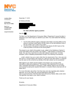
D. Technical Debt across Technologies
In Figure 8 we present the amount of technical debt per
line of code across different technologies. Java systems are
shown to have the lowest technical debt—averaging e1.6
per LOC, while ABAP and PL/SQL are the two technologies with the highest technical debt—averaging e15.4
and e13.5 per LOC respectively. Following ABAP and
PL/SQL, COBOL systems have the third highest technical
debt, averaging e4 per LOC.
These findings contradict with the report published by
CAST [12]. CAST reported that ABAP and COBOL systems have the lowest technical debt per KLOC, while Java
systems were found to have the highest technical debt.
Considering plausible differences in the method used to
calculate technical debt discrepancies in the absolute terms
are expected. However, in relative terms it is counter intuitive
to learn that modern technologies such as .NET and Java
were found by CAST to have higher technical debt compared
to old technologies like COBOL. In our approach, old
technologies such as COBOL are found to have higher
technical debt, which is closer to intuition.
V. D ISCUSSION
In this paper we have presented three models to assess
the value of software. We apply the models to a large
collection of software and found that the results obtained by
the three models are quite similar. The question concerning
which valuation model to use then becomes a matter of
preference. Model 1 and 2 are quite similar in nature.
However, one would prefer Model 1 if a more realistic
estimate, which takes into account factors influencing repair
costs, is preferred. Model 2 will generally be chosen for its
simplicity. Model 3 has a different nature, and one would
choose this model if a repair scenario is not an option.
To understand how practitioners think of the valuation
models, we have conducted several case studies reported
in [7]. We identify important insights concerning their views
on the software valuation models. Firstly, we found that
practitioners generally agree that an objective framework for
assessing software value is needed and still lacking in the
current practice. Secondly, they consider the three models as
complementary to each other in looking at software value
from different point of views. Finally, the proposed models
are seen as an improvement of the current valuation practice,
which is based on total development cost.
Several CFOs that participated in the study considered the
models as an important instrument for valuation during due
diligence. The buyer can make a good assessment of the
value of software assets in a quick and simple way.
Technical Debt per Line of Code
Software Value per Line of Code - Model 1
20
20
15
EUROS / LOC
EUROS / LOC
15
10
10
5
5
0
0
ABAP
COBOL
C++
C#
Java
Mixed
ABAP
PL/SQL
EUROS / LOC
Figure 8.
C#
Java
Mixed
PL/SQL
Technical debt per line of code across technologies
15
VI. R ELATED W ORK
10
The work of Sneller and Bots [13] is a review of quantitative IT value research in which all IT value quantitative
research and methods are listed and compared after the
year 2000. In the paper, IT value is defined as research
that impacts financial performance of IT. The forty research
papers found by Sneller and Bots can be separated in four
categories; capital market theory, microeconomic theory,
resource-based view of the firm and analysis of financial
statements. Generalizable from these studies is that research
focuses on the impact of IT on financial aspects. For
example, IT’s effect on equity price or firms productivity
or financial ratios like ROI and ROA. Concluding from the
study, IT value research focuses on financial return rather
than risk-reward trade-offs.
To the best of our knowledge little work has been done to
define and measure software value based on intrinsic values
and actual measurements. In this section, the discussion
on related work is focused on proposed approaches to
quantify intrinsic software value. At present, software value
is determined based on a sum of costs. Ben-Menachem and
Gavious disagree with this method, and argue intrinsic value
of a software asset cannot be only the cost incurred [14].
Example given is a software module that serves as an
interface between several systems. Although the module has
a relatively low production cost but the high degree of reuse
of the module should enhance its value. A model is proposed
to calculate the real intrinsic value based on total costs and
premium/discount factors.
The premium/discount factors are based on a software
sensitivity theory designed by the authors. Software
sensitivity is used to calculate how software change
can affect the business environment. Four quantifiable
parameters affect sensitivity: reuse count, complexity,
update difficulty, and interface implementation. Reuse
count refers to the quantity of uses for this module.
Complexity and update difficulty are technical concepts
5
0
-5
ABAP
COBOL
C++
C#
Java
Mixed
PL/SQL
Technology
Software Value per Line of Code - Model 3
15
EUROS / LOC
C++
Technology
Technology
Software Value per Line of Code - Model 2
COBOL
10
5
0
-5
ABAP
COBOL
C++
C#
Java
Mixed
PL/SQL
Technology
Figure 7. Software value across technologies calculated using the proposed
software valuation models (1 man-year = 100,000 euros).
When rationalizing a software landscape, software valuation may be a guiding principle in investment decisions.
Instead of examining the incurred development costs, systems may be preferred on the basis of the required repair
costs and future maintenance costs. The proposed valuation
models are very suitable for comparing software portfolios
of various organizations. This makes it possible to benchmark organizations in an objective way.
referring to how the module is constructed. Interface
implementation refers to the connection a module can have
to several systems. There are several limitations in the
model proposed by Ben-Menachem and Gavious. Firstly,
the model does not seem to clearly explain the underlying
aspects behind software valuation, which make it difficult
to use for root-cause analyses. Secondly, the model is
not validated. Therefore, it is very difficult to rely on
the conceptual equation in the paper of Ben-Menachem
and Gavious. Thirdly, the final result is based on several
expert estimates of the software system that could be biased.
VII. C ONCLUSION AND F UTURE W ORK
in software will give a more comprehensive view of the
value of software for organizations.
R EFERENCES
[1] B. Boehm and P. Papaccio, “Understanding and controlling
software costs,” Software Engineering, IEEE Transactions on,
vol. 14, no. 10, pp. 1462 –1477, oct 1988.
[2] N. Melville, K. L. Kraemer, and V. Gurbaxani, “Review:
Information technology and organizational performance: An
integrative model of IT business value,” MIS Quarterly,
vol. 28, no. 2, pp. 283–322, 2004.
[3] Financial Accounting Standards Board (FASB), “U.S. GAAP
Codification of Accounting Standards, Codification Topic
350: Intangibles-Goodwill and Other (ASC 350),” 2009.
In this paper we present three models to determine software value based on the notions of technical debt. We use
Rebuild Value (the cost to rebuild a system using a similar
technology) as the base value of software. Impairment to
this base value is done based on the notions of technical
debt. The first model uses repair cost to adjust the value
of software. The second model uses a similar approach but
neglecting project environmental factors to impair software
value. Finally, the third model uses technical interest (extra
costs spent on maintenance) as an impairment factor of
software value.
We apply the three valuation models to 367 proprietary
software and learn the following insights:
[4] International Financial Report Standards (IFRS), “International Accounting Standard 38 (IAS 38), Intangible Assets,”
First issued 1998, revised 2004, amendment 2008.
There is no significant difference in the results provided by the three models. The average software value
resulted from the three model is around e7 per LOC.
Valuation model that is based on repair effort is the
most lenient, and it is due to its recognition of factors
that might influence productivity in performing rework.
Across the three models, C# systems are found to have
the highest value, averaging e10 per LOC.
Java systems are found to have the lowest technical
debt, averaging e1.6 per LOC.
[8] W. Cunningham, “The WyCash portfolio management system,” ACM SIGPLAN OOPS Messenger, vol. 4, no. 2, pp.
29–30, 1993.
•
•
•
•
Future work is needed to investigate the extent to which
the results given by the proposed valuation models differ
from that of conservative approach that is based on the actual
costs spent during software development. Performing such
an investigation in proprietary software projects might be
difficult due to the sensitivity of the required information.
Nevertheless, this endeavor is worth investigating as it might
reveal whether there is a general trend of overstating the
value of software. More research is also needed to broaden
the scope of technical debt to cover more aspects beyond
maintainability such as reliability and usability.
Finally, further research should look into the business
value of software—the business and financial benefits obtained from running software systems. Combining the notions of production value, business value, and technical debt
[5] R. G. Walker and G. R. Oliver, “Accounting for expenditure
on software development for internal use,” Abacus, vol. 41,
no. 1, pp. 66–91, 2005.
[6] D. Aboody and B. Lev, “The value relevance of intangibles:
The case of software capitalization,” Journal of Accounting
Research, vol. 36, no. 1998, p. 161, 1998.
[7] J. de Groot, “Incorporating software quality in the capitalization of software as an asset,” 2011, MSc thesis, Leiden
University.
[9] A. Nugroho, J. Visser, and T. Kuipers, “An empirical model
of technical debt and interest,” in Proceeding of the 2nd
International Workshop on Managing Technical Debt. ACM,
2011, pp. 1–8.
[10] I. Heitlager, T. Kuipers, and J. Visser, “A practical model
for measuring maintainability,” in Quality of Information and
Communications Technology, 6th International Conference on
the Quality of Information and Communications Technology,
QUATIC 2007, Lisbon, Portugal, September 12-14, 2007,
Proceedings, R. J. Machado, F. B. e Abreu, and P. R.
da Cunha, Eds. IEEE Computer Society, 2007, pp. 30–39.
[11] R. Baggen, J. Correia, K. Schill, and J. Visser, “Standardized
code quality benchmarking for improving software maintainability,” Software Quality Journal, pp. 1–21, 2011.
[12] CAST, “CAST report on application software health,” 2012.
[13] L. Sneller and J. Bots, “A review of quantitative IT value
research,” Proceedings of the 13th European conference on
IT evaluation, pp. 444–452, 2006.
[14] M. Ben-Menachem and I. Gavious, “Accounting software assets: A valuation model for software,” Journal of Information
Systems, vol. 21, pp. 117–132, 2007.