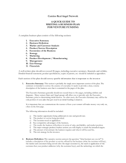
"Why JobshopLean?"
This is the original full-length version of the abridged article
that appeared in the December 2011 issue of
THE FABRICATOR (pages 42-44).
Product Mix Segmentation using P-Q-$ Analysis
Shahrukh A. Irani
Department of Integrated Systems Engineering
The Ohio State University
Columbus, OH43210
Background
Although P-Q Analysis (P= Part, or Product, Q= Quantity, or Production Volume) is a simple and effective
method for product mix segmentation, P-Q-$ Analysis ($= Sales, or Profit, or Revenue) simultaneously
considers two criteria to rank order and classify products into different segments. P-Q Analysis identifies
at most three product segments (High, Medium and Low Volume) in the product mix of a jobshop.
Whereas, P-Q-$ Analysis could identify up to four different segments in the same product mix. Ideally,
each business segment ought to be served using a different combination of facility layout, manufacturing
technology, workforce skills, management strategy, etc.!
Justification for this Strategy
When implementing Lean in a high-variety low-volume (HVLV) manufacturing facility, especially in a
jobshop where small batches of high-priced products are often the norm, we could be erring by focusing on
the Value Streams of products that belong in the High-Volume segment that is typically identified by P-Q
Analysis. There are two reasons why P-Q Analysis could often select the wrong products to focus on: (i)
the High-Volume products do not belong in the High-Revenue segment and (ii) the products in the (LowVolume, High-Revenue) segment that are often profitable are ignored by P-Q Analysis! Cash flow in any
business can be improved by (1) completing high-value orders in the shortest period of time and (2)
reducing the Seven Types of Waste that decrease margins for the low-volume but high-margin parts.
From the perspective of Flow, three types of operational costs – Transportation, WIP (work-in-process
inventory) and Queuing – increase manufacturing costs. Two costs – Transportation and Queuing – are
heavily dependent on production volumes and container sizes; but, WIP cost is heavily dependent on
product value, which is usually reflected in the Sales earned by each product. So, instead of focusing on a
sample of products selected using a single criterion – Quantity – the P-Q- Analysis method recommends
focusing on a sample of products that is drawn from several segments of the product mix – (High-Volume,
High-Revenue), (High-Volume, Low-Revenue) and (Low-Volume, High Revenue). As shown in Figure 1,
P-Q-$ Analysis creates a two-dimensional scatterplot for the entire product mix of any jobshop as follows:
 The horizontal axis (X) represents Quantity (or Volume).
 The vertical axis (Y) represents Revenue (or Profit Margin).
 Every point in the scatterplot represents a particular product.
 Q* is the threshold value of Q that separates Low-Volume products from High-Volume products.
Similarly, R* is the threshold value of Sales that separates the Low-Revenue products from the HighRevenue products. There are simple as well as sophisticated methods for choosing the points – Q* and
R* – on the two axes. Those methods are beyond the scope of this introductory article. If we draw a
vertical line on the X axis at Q* and a horizontal line on the Y axis from R*, then the P-Q-$ scatterplot
gets divided into four quadrants. Each product will lie in any one of the four quadrants, depending on
its (Q, $) values. The four quadrants are (High-Quantity, High-Revenue), (Low-Quantity, HighRevenue), (Low-Quantity, Low-Revenue) and (High-Quantity, Low-Revenue). Each quadrant defines
a product mix “segment” that, ideally, ought to be managed as a separate business and be produced in a
separate area of the facility with a suitable layout for that area, manufacturing technology, workforce
skills and management strategy!
Low

High
80000
70000
60000
Revenue
50000
High
40000

30000
20000

R*
Low
10000
0
0
2000
4000
6000
Q*
8000
10000
12000

Quantity
Figure 1 P-Q-$ Analysis Scatter Plot of the Product Mix in a Hypothetical Jobshop
Case Study
Table 1 shows the input data from an actual project used for P-Q Analysis (where P= Part or Product and
Q= Quantity or Production Volume). Typically, the “Quantity” (# of pieces shipped) and “Revenue” ($
earned) for each part are for a year, or longer production horizon. The “Routing” is the sequence of
workcenters that a part must visit ex. Part No. 1 (80-A37353) has the routing:
17→6→2→11→10→29→54→55. Figure 1 and Table 2 are the graphical and tabular versions,
respectively, of the P-Q Analysis output that would be used to segment the product mix of any jobshop. In
Figure 1 the Parts are sequenced from left-to-right along the X-axis in order of decreasing value of Quantity
of each (individual) part; whereas, the Y-axis on the left side of the graph shows the Quantity of each
(individual) part and the Y-axis on the right side of the graph shows the Aggregate Quantity for any group
of parts. In this particular example, the curve in Figure 1 is “sharp” and the points where the curve has
sharp bends are potential cut-off points between different segments of the product mix, such as HighVolume (Runners), Medium-Volume (Repeaters) and Low-Volume (Strangers) segments. In Table 2,
where the parts have been sorted in order of decreasing value of Quantity, the Total Aggregate Quantity for
a sample of parts comprised of the first 23 parts in the total list of 79 is 1411592 (see Row # 23 in the table)
accounts for about 80% of the Total Aggregate Quantity for all 79 parts (which is 1766478). So, using
Figure 1 and Table 2, we could segment the product mix into at least two segments, one comprised of the
top 23 parts and the other containing the remaining 56 parts.
Next, instead of using Q, if we used Sales and did a P-$ Analysis, the Pareto sort of the products would
have sequenced them by decreasing value of Sales, as shown in Table 3 and plotted in Figure 2.
Are the two samples of parts chosen using either Q (Volume) or $ (Sales) the same? No! So why not
enhance the Pareto sorting algorithm to simultaneously incorporate both Q and $? Here is how to do it --Using the columns of data “Part”, “Quantity” and “Revenue” in Table 1, first produce the scatterplot that
appears in Figure 3. Even if you did no further analysis and eyeballed Figure 3, you could produce a
segmentation of the product mix as shown in Figure 4. In that figure, the scatter plot suggests that the
product mix of this jobshop could have three segments – (High-Volume Low-Revenue), (Low-Volume
High-Revenue) and (Low-Volume Low-Revenue). So, if we had we relied only on PQ Analysis (Table 2),
we would have ignored the products in the High Revenue Low Volume segment. And, if we had relied
only on P$ Analysis (Table 3), we would have ignored the products in the Low Revenue High Volume
segment.
Now, for the purpose of this article, you could do something better than just eyeballing to create a 4quadrant split of the product mix as follows: Locate the point (R*) on the Revenue axis that corresponds to
the Revenue value for Part #80-4030007296090 (R*) which is the last part to be included in the Pareto sort
to select the P$ Analysis sample. Draw a vertical line through this point. Similarly, on the Quantity axis,
locate the point (Q*) that corresponds to the Quantity Value for Part #80-121009-00 which is the last part
to be included in the Pareto sort to select the PQ Analysis sample. Draw a horizontal line through this
point. Thereby, you will split the PQ$ Analysis scatterplot into four quadrants. If you desire to know the
exact PQ$ Analysis results produced by the proprietary algorithm in the PFAST software that we use to
implement JobshopLean, please send me an email at [email protected] to request that information.
Managing a Jobshop’s Different Product Mix Segments Differently
How does one translate the results obtained using this LAT into improvement projects (or kaizen events),
management policies, strategic plans, etc.? Here are some examples of the follow-on projects that could be
undertaken using the PQ$ Analysis results:
Market Diversification: If you study Figure 3, this particular jobshop does not have a single part # in the
(High Revenue, High Quantity) quadrant. That figures because a jobshop’s niche is not low-mix highvolume manufacturing! However, creative jobshop owners do not pass up on any opportunity to accept a
Long Term Contract from a defense prime or an OEM to supply a single part (or a well-defined part
family) that will be ordered on a consistent basis (think takt time!) all through the year, maybe even for a
few years! For example, one machine shop set up a stand-alone robotic cell for a single part ordered by a
defense prime. Another machine shop installed a dedicated flexible manufacturing cell operated by a
single operator to produce a single part for an automotive OEM in their state.
Facility Layout, Virtual Cells and Workforce Training (and Compensation too!): A manufacturer of
hydraulic pipes and couplings produced 2,000 stock keeping units (SKUs) with 48 hours lead-time
customers. The manufacturer was finding it increasingly costly and difficult to consistently achieve this
lead-time. Analysis showed over 50% of sales came from only 92 products, or less than 5% of the entire
product mix. The other products were ordered infrequently in small quantities, even as single items.
Armed with this information, the company decided it needed two types of factory: a high-volume repetitive
facility and a flexible job shop. However, it was not cost effective to build two factories. Or even to
physically separate the equipment. The company worked out what equipment would be needed for highvolume products in a fixed sequence. This equipment was painted green. Employees for this equipment
were selected based on their preference to work routines. They were given green overalls. The remaining
equipment was painted beige. Employees were selected on their preference to tackle difficult and complex
situations, in their case, lots of setups and unusual machining issues. They were given beige overalls.
Although the equipment and staff were totally intermingled on the shop floor, each business operated
totally differently. The green factory had fixed hours of work, JIT deliveries and improvement activities
focused on achieving faster cycle times and increased productivity. The beige factory had hours of work
that varied according to the level of demand each week. Materials were only purchased when required.
Improvement activities focused on flexibility and responsiveness. This company succeeded in creating and
operating two businesses under the same roof, even each business had different policies, procedures and
appropriate performance metrics. For complete details on this eye-opening case study, please read Page 27
“One Business or Two?’ in this book --- Glenday, I. (2005). Breaking Through to Flow: Banish Fire
Fighting and Increase Customer Service. Ross-on-Wye, United Kingdom: Lean Enterprise Academy.
ISBN 0-9551473-0-1.
Vendor Selection, Purchasing Management and Inventory Control: High-volume products, which
allow production batch sizes to match a Make-To-Stock inventory policy, also influence how far the
suppliers are from the company location, and for FTL (full truck loads) at time of delivery. In contrast,
high-revenue orders made from rare metals like titanium (which is not easily available if shipped from, say,
China) merit keeping a very close watch on onhand inventory levels, supplier lead times, market price, etc.
Priority Scheduling of Orders Loaded on Bottleneck Resources: By knowing which products are of
high-value but to be delivered by certain due dates, as opposed which orders are being run to replenish
kanban-triggered onhand stock, appropriate inventory control systems can be used for products in different
segments. In fact, products in the (High-Volume, Low-Revenue) segment could be outsourced but labeled
at the time of shipment by the company selling them to customers. What about shopfloor scheduling? The
color of the paperwork, containers, etc. associated with a high-revenue order could be different from the
paperwork for the other orders, so everybody on the shop gives a higher priority to minimizing WIP
corresponding to that category of orders.
Equipment Purchases: The value and volume of production of different products easily influences the
flexibility and sophistication of manufacturing equipment. High-volume assembly facilities are
increasingly embracing “right-sized automation” i.e. equipment that is designed for producing a welldefined low mix of products in a well-defined range of volumes. On the other hand, most jobshops that I
know, who struggle to hire and retain multi-skilled equipment operators, are the first to purchase flexible
multi-function single-setup machines, some capable of lights-out operation.
About the Next Column
In the next column, we will conclude this series on the PQR$T Analysis approach to accurate product mix
segmentation as a crucial starting point for jobshops on their Lean journey. In my next column, I will
describe PQT Analysis, a method for Product Mix Segmentation that considers both QUANTITY and
DEMAND REPEATABILITY for any product to segment the entire product mix of a jobshop, especially
when 1000+ routings are involved. PQ Analysis, which is based on the old and obsolete Pareto Law (or
80-20 Rule), fails to consider how many times any product is ordered, the size and variability in order sizes,
and the time interval between consecutive orders. Which is why PQT Analysis, instead of PQ Analysis, is
a preferred method for identifying the Runners, Repeaters and Strangers in a jobshop’s product mix.
Shahrukh Irani, Ph.D., [email protected] is an Associate Professor at The Ohio State University’s
Department of Integrated Systems Engineering www.ise.osu.edu, 210 Baker Systems Engineering,
1971 Neil Ave., Columbus, OH 43210-1271, 614-688-4685. His work at The Ohio State
University was supported by the Defense Logistics Agency through the cost-shared Forging
Advanced Systems and Technologies (FAST) Manufacturing Technology (ManTech)
Program. Support is provided by the Defense Logistics Supply Center in Philadelphia, PA, and
Headquarters Defense Logistics Agency at Fort Belvoir, VA. The FAST Program focuses on
lead-time and cost reduction within forging supply chains through the teamed relationship of
Advanced Technology International and the Forging Industry Association.
Table 1 Input Data for P-Q Analysis
No.
1
2
3
4
5
6
7
8
9
10
11
12
13
14
15
16
17
18
19
20
21
22
23
24
25
26
27
28
29
30
31
32
33
34
35
36
37
38
39
40
41
42
43
44
45
46
47
48
49
50
51
52
53
54
55
56
57
58
59
60
61
62
63
64
65
66
67
68
69
70
71
72
73
74
75
76
77
78
79
Part
80-A37353
80-C27416-1
80-C27416-2
80-C46806-1
80-C55581
80-C558-1
80-D8097
80-B113-1001
80-4003111
80-4009121
80-4009262
80-4009263
80-4009270
80-4010346
80-4010348
80-4010349
80-4010350
80-4010351
80-4010352
80-4011714
80-4011725
80-4012169
80-4012174
80-4012179
80-4012212
80-4012213
80-4030339
80-4030341
80-4035144
80-4035149
80-4039260
80-4041707
80-4059989
80-4067179
80-4030011870964
80-150T084LT
80-G121-1002
80-NL150T060LT
80-NL150T072LT
80-NL150T084LT
80-NL150T096LT
80-NL150T120LT
80-3249869
80-121009-00
80-121188-002
80-121189
80-671391
80-121018-00
80-121148
80-121387
80-ULC0200
80-35-B357
80-27750-01
80-37355-1072
80-37355-1084
80-051-1
80-191820
80-522500
80-551500
80-S113-1001
80-S113-1004
80-27708-302UP
80-9033023-303
80-9627712-301UP
80-9627713-301UP
80-9627714-301UP
80-9627715-301UP
80-9627716-301UP
80-3260-041
80-3260-0980
80-3260-503
80-671635-00
80-4030007296089
80-4030007296090
80-4030007296091
80-4030007296094
80-27377
80-921790
80-W101-2006
Quantity
728
1456
5614
4354
1750
1526
756
48132
4900
30800
5600
39886
32900
117614
21000
12600
38500
19600
7000
28000
16800
33362
113400
133070
1400
4144
65198
53200
5600
28252
1400
42000
3850
26502
39256
1344
280
1764
1540
644
168
112
28014
29288
32200
7014
147000
47950
35350
3220
2800
132314
15428
1204
952
48580
26866
1652
3724
39732
364
8540
36848
1022
1050
1078
1022
1022
2828
1512
182
75012
168
1456
6356
9240
14112
4914
462
Revenue
47320
124054
495992
362474
151284
131922
133882
186116
41216
151228
27048
176302
126994
379806
69300
43092
148610
86632
34790
91560
119448
98756
324324
377916
10682
34846
117208
140980
14952
86170
6062
180180
33306
757428
1618932
587664
138768
632744
591752
281596
83258
68572
179200
171332
202860
47348
658560
275716
143444
27720
31556
697298
931854
501774
447062
255052
100744
8428
29050
39732
70532
1952230
922670
192276
462378
360430
423766
139258
569842
157024
48342
466340
38892
234346
757190
574084
69286
526120
445858
17
17
17
17
17
17
17
17
1
1
1
1
1
1
1
1
1
1
1
1
1
1
1
1
1
1
1
1
1
1
1
1
1
17
17
17
17
17
17
17
17
17
17
17
17
17
17
17
1
17
17
17
17
17
17
17
17
17
17
17
17
17
57
17
17
17
17
17
17
17
17
17
17
17
17
17
17
17
17
6
6
6
6
6
6
6
56
57
57
57
57
57
57
57
57
57
57
57
26
57
26
26
26
26
26
27
27
28
28
28
57
26
39
39
6
6
6
6
6
6
6
56
39
39
39
16
39
50
39
39
1
39
6
6
1
16
16
16
16
16
39
54
6
6
6
6
6
6
6
6
3
3
3
3
3
16
3
6
2
2
2
2
2
2
2
57
25
25
25
25
25
25
25
25
25
25
25
57
25
57
57
57
57
57
9
9
50
50
50
25
57
40
40
2
2
2
2
2
2
2
1
40
40
40
11
40
26
40
40
57
40
2
2
26
11
11
11
11
11
40
57
56
56
56
56
56
2
2
2
7
7
7
7
7
11
7
2
11
11
11
11
11
11
11
54
52
52
52
52
52
52
52
52
52
52
52
52
52
52
52
52
52
52
57
57
27
27
27
52
52
26
21
7
7
7
7
7
7
7
17
21
21
21
10
21
27
21
21
4
42
7
7
4
10
10
10
10
10
16
55
16
16
16
16
16
11
11
11
12
12
12
12
12
10
12
42
10
10
10
10
10
10
10
29
29
29
29
29
29
29
48
48
48
48
48
48
48
48
48
48
48
48
48
48
48
48
48
48
48
48
48
48
48
48
48
57
22
12
12
12
12
12
12
12
29
22
22
22
26
22
55
22
22
54
41
12
12
54
26
26
26
57
57
9
55
55
55
55
55
55
55
55
55
55
55
55
55
55
55
55
55
55
11
11
11
11
11
10
10
10
26
8
8
8
8
26
8
33
55
55
55
55
55
54
53
8
8
8
8
8
8
8
26
55
55
55
4
55
54
54
54
54
54
54
54
Routings
55
55
55
55
55
55
55
57
29
42
42
42
42
42
42
42
54
55
28
41
41
41
41
41
41
41
57
4
57
57
57
57
57
57
57
48
55
55
55
55
55
55
55
55
54
55
55
55
55
55
55
55
3
8
8
55
29
29
29
53
53
11
7
42
42
12
41
41
57
57
57
28
28
28
55
55
10
27
27
27
48
48
48
39
40
57
54
10
10
10
10
10
29
29
29
4
4
4
4
4
4
54
41
6
6
6
6
6
28
28
28
55
54
54
54
54
55
29
54
7
7
7
7
7
54
54
54
12
12
12
12
12
57
57
57
8
8
8
8
8
55
55
55
54
54
54
54
54
29
29
29
29
4
4
4
4
55
55
55
55
28
57
4
4
55
55
57
57
57
57
57
54
54
54
54
54
53
53
53
53
53
8
8
8
8
8
55
55
55
55
55
Figure 1 P-Q Analysis
High-Volume Parts
Medium-Volume Parts
Low-Volume Parts
Table 2 Prioritization of Products using only P-Q Analysis
No.
1
2
3
4
5
6
7
8
9
10
11
12
13
14
15
16
17
18
19
20
21
22
23
24
25
26
27
28
29
30
31
32
33
34
35
36
37
38
39
40
41
42
43
44
45
46
47
48
49
50
51
52
53
54
55
56
57
58
59
60
61
62
63
64
65
66
67
68
69
70
71
72
73
74
75
76
77
78
79
Part
80-671391
80-4012179
80-35-B357
80-4010346
80-4012174
80-671635-00
80-4030339
80-4030341
80-051-1
80-B113-1001
80-121018-00
80-4041707
80-4009263
80-S113-1001
80-4030011870964
80-4010350
80-9033023-303
80-121148
80-4012169
80-4009270
80-121188-002
80-4009121
80-121009-00
80-4035149
80-3249869
80-4011714
80-191820
80-4067179
80-4010348
80-4010351
80-4011725
80-27750-01
80-27377
80-4010349
80-4030007296094
80-27708-302UP
80-121189
80-4010352
80-4030007296091
80-C27416-2
80-4009262
80-4035144
80-921790
80-4003111
80-C46806-1
80-4012213
80-4059989
80-551500
80-121387
80-3260-041
80-ULC0200
80-NL150T060LT
80-C55581
80-522500
80-NL150T072LT
80-C558-1
80-3260-0980
80-4030007296090
80-C27416-1
80-4012212
80-4039260
80-150T084LT
80-37355-1072
80-9627714-301UP
80-9627713-301UP
80-9627712-301UP
80-9627715-301UP
80-9627716-301UP
80-37355-1084
80-D8097
80-A37353
80-NL150T084LT
80-W101-2006
80-S113-1004
80-G121-1002
80-3260-503
80-4030007296089
80-NL150T096LT
80-NL150T120LT
Quantity
147000
133070
132314
117614
113400
75012
65198
53200
48580
48132
47950
42000
39886
39732
39256
38500
36848
35350
33362
32900
32200
30800
29288
28252
28014
28000
26866
26502
21000
19600
16800
15428
14112
12600
9240
8540
7014
7000
6356
5614
5600
5600
4914
4900
4354
4144
3850
3724
3220
2828
2800
1764
1750
1652
1540
1526
1512
1456
1456
1400
1400
1344
1204
1078
1050
1022
1022
1022
952
756
728
644
462
364
280
182
168
168
112
Agg. Qty.
147000
280070
412384
529998
643398
718410
783608
836808
885388
933520
981470
1023470
1063356
1103088
1142344
1180844
1217692
1253042
1286404
1319304
1351504
1382304
1411592
1439844
1467858
1495858
1522724
1549226
1570226
1589826
1606626
1622054
1636166
1648766
1658006
1666546
1673560
1680560
1686916
1692530
1698130
1703730
1708644
1713544
1717898
1722042
1725892
1729616
1732836
1735664
1738464
1740228
1741978
1743630
1745170
1746696
1748208
1749664
1751120
1752520
1753920
1755264
1756468
1757546
1758596
1759618
1760640
1761662
1762614
1763370
1764098
1764742
1765204
1765568
1765848
1766030
1766198
1766366
1766478
Agg. Qty. %
8.3
15.9
23.3
30
36.4
40.7
44.4
47.4
50.1
52.8
55.6
57.9
60.2
62.4
64.7
66.8
68.9
70.9
72.8
74.7
76.5
78.3
79.9
81.5
83.1
84.7
86.2
87.7
88.9
90
91
91.8
92.6
93.3
93.9
94.3
94.7
95.1
95.5
95.8
96.1
96.4
96.7
97
97.2
97.5
97.7
97.9
98.1
98.3
98.4
98.5
98.6
98.7
98.8
98.9
99
99
99.1
99.2
99.3
99.4
99.4
99.5
99.6
99.6
99.7
99.7
99.8
99.8
99.9
99.9
99.9
99.9
100
100
100
100
100
Figure 2 P- $ Analysis
P-$ Analysis
2500000
25000000
High-Revenue Parts
2000000
20000000
1500000
15000000
Aggregate Revenue
Revenue
Revenue
Agg Revenue
1000000
Medium-Revenue Parts
10000000
Low-Revenue Parts
500000
5000000
0
0
Parts
Table 3 Prioritization of Products using only P-$ Analysis
No.
Revenue
Agg. Rev.
1
80-27708-302UP
1952230
1952230
8.69
2
80-4030011870964
Part
1618932
3571162
Agg. Rev. %
15.89
3
80-27750-01
931854
4503016
20.04
4
80-9033023-303
922670
5425686
24.14
5
80-4067179
757428
6183114
27.51
6
80-4030007296091
757190
6940304
30.88
7
80-35-B357
697298
7637602
33.98
8
80-671391
658560
8296162
36.91
9
80-NL150T060LT
632744
8928906
39.73
10
80-NL150T072LT
591752
9520658
42.36
11
80-150T084LT
587664
10108322
44.98
12
80-4030007296094
574084
10682406
47.53
13
80-3260-041
569842
11252248
50.07
14
80-921790
526120
11778368
52.41
15
80-37355-1072
501774
12280142
54.64
16
80-C27416-2
495992
12776134
56.85
17
80-671635-00
466340
13242474
58.92
18
80-9627713-301UP
462378
13704852
60.98
19
80-37355-1084
447062
14151914
62.97
20
80-W101-2006
445858
14597772
64.95
21
80-9627715-301UP
423766
15021538
66.84
22
80-4010346
379806
15401344
68.53
23
80-4012179
377916
15779260
70.21
24
80-C46806-1
362474
16141734
71.82
25
80-9627714-301UP
360430
16502164
73.43
26
80-4012174
324324
16826488
74.87
27
80-NL150T084LT
281596
17108084
76.12
28
80-121018-00
275716
17383800
77.35
29
80-051-1
255052
17638852
78.48
30
80-4030007296090
234346
17873198
79.53
31
80-121188-002
202860
18076058
80.43
32
80-9627712-301UP
192276
18268334
81.28
33
80-B113-1001
186116
18454450
82.11
34
80-4041707
180180
18634630
82.91
35
80-3249869
179200
18813830
83.71
36
80-4009263
176302
18990132
84.50
37
80-121009-00
171332
19161464
85.26
38
80-3260-0980
157024
19318488
85.96
39
80-C55581
151284
19469772
86.63
40
80-4009121
151228
19621000
87.30
41
80-4010350
148610
19769610
87.96
42
80-121148
143444
19913054
88.60
43
80-4030341
140980
20054034
89.23
44
80-9627716-301UP
139258
20193292
89.85
45
80-G121-1002
138768
20332060
90.47
46
80-D8097
133882
20465942
91.06
47
80-C558-1
131922
20597864
91.65
48
80-4009270
126994
20724858
92.21
49
80-C27416-1
124054
20848912
92.77
50
80-4011725
119448
20968360
93.30
51
80-4030339
117208
21085568
93.82
52
80-191820
100744
21186312
94.27
53
80-4012169
98756
21285068
94.71
54
80-4011714
91560
21376628
95.11
55
80-4010351
86632
21463260
95.50
56
80-4035149
86170
21549430
95.88
57
80-NL150T096LT
83258
21632688
96.25
58
80-S113-1004
70532
21703220
96.57
59
80-4010348
69300
21772520
96.88
60
80-27377
69286
21841806
97.18
61
80-NL150T120LT
68572
21910378
97.49
62
80-3260-503
48342
21958720
97.70
63
80-121189
47348
22006068
97.91
64
80-A37353
47320
22053388
98.13
65
80-4010349
43092
22096480
98.32
66
80-4003111
41216
22137696
98.50
67
80-S113-1001
39732
22177428
98.68
68
80-4030007296089
38892
22216320
98.85
69
80-4012213
34846
22251166
99.01
70
80-4010352
34790
22285956
99.16
71
80-4059989
33306
22319262
99.31
72
80-ULC0200
31556
22350818
99.45
73
80-551500
29050
22379868
99.58
74
80-121387
27720
22407588
99.70
75
80-4009262
27048
22434636
99.82
76
80-4035144
14952
22449588
99.89
77
80-4012212
10682
22460270
78
80-522500
8428
22468698
99.97
79
80-4039260
6062
22474760
100.00
99.94
Figure 3 P-Q-$ Analysis
Figure 4 How P-Q-$ Analysis Combines P-Q Analysis and P-$ Analysis
160000
140000
120000
Runners & Repeaters
in P-Q Analysis?
Included in Sample
80000
Excluded from Sample
Completely ignored by
P-Q Analysis?
60000
40000
20000
Strangers in P-Q Analysis?
Revenue
25
00
00
0
20
00
00
0
15
00
00
0
10
00
00
0
50
00
00
0
0
Quantity
100000