1. technology and computing

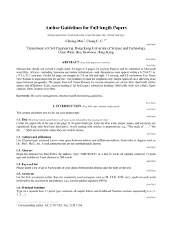
The What, How, and Why of Wavelet Shrinkage Denoising
Carl Taswell∗
Computational Toolsmiths, Stanford, CA 94309-9925
Abstract
Principles of wavelet shrinkage denoising are reviewed. Both 1-D and 2-D examples are
demonstrated. The performance of various ideal and practical Fourier and wavelet based denoising procedures are evaluated and compared in a new Monte Carlo simulation experiment.
Finally, recommendations for the practitioner are discussed.
1
Some Opposing Viewpoints
Applied scientists and engineers who work with data obtained from the real world know that
signals do not exist without noise. Under ideal conditions, this noise may decrease to such negligible
levels, while the signal increases to such significant levels, that for all practical purposes denoising
is not necessary. Unfortunately, the noise corrupting the signal, more often than not, must be
removed in order to recover the signal and proceed with further data analysis. Should this noise
removal take place in the original signal (time-space) domain or in a transform domain? If the
latter, should it be the time-frequency domain via the Fourier transform or the time-scale domain
via the wavelet transform?
Enthusiastic supporters have described the development of wavelet transforms as revolutionizing
modern signal and image processing over the past two decades. Conservative observers, however,
would simply recognize this new field as contributing additional useful tools to a growing toolbox
of transforms, in fact, an old toolbox that has had an evolving history over the past two centuries.
For a review of available software libraries and an introduction to some of the wavelet literature,
refer to the survey by Shearman [7].
Even more zealous advocates have claimed that a particular wavelet method called wavelet
shrinkage denoising “offers all that we might desire of a technique, from optimality to generality”
[4, page 312]. Inquiring skeptics, however, might be loath to accept these claims based on asymptotic theory without persuasive evidence from real-world experiments. Fortunately, a burgeoning
literature is now addressing these concerns, and leading to a more realistic appraisal of the utility
of wavelet shrinkage denoising.
2
A Simple Explanation and a 1-D Example
But what is wavelet shrinkage denoising? First, it is not smoothing (despite the use by some
authors of the term smoothing as a synonym for the term denoising). Whereas smoothing removes
high frequencies and retains low frequencies, denoising attempts to remove whatever noise is present
and retain whatever signal is present regardless of the frequency content of the signal. For example,
∗
Email: [email protected]; Website: www.toolsmiths.com; Tel/Fax: 650-323-4336/5779. Technical Report
CT-1998-09: original 10/13/98, revision 1/25/99.
2
Taswell: Wavelet Shrinkage Denoising.
when we denoise music corrupted by noise, we would like to preserve both the treble and the bass.
Second, it is denoising by shrinking (i.e., nonlinear soft thresholding) in the wavelet transform
domain. Third, it consists of three steps: 1) a linear forward wavelet transform, 2) a nonlinear
shrinkage denoising, and 3) a linear inverse wavelet transform. Because of the nonlinear shrinking of
coefficients in the transform domain, this procedure is distinct from those denoising methods that
are entirely linear. Finally, wavelet shrinkage denoising is considered a non-parametric method.
Thus, it is distinct from parametric methods [6] in which parameters must be estimated for a
particular model that must be assumed a priori. (For example, the most commonly cited parametric
method is that of using least squares to estimate the parameters a and b in the model y = ax + b.)
Figure 1 displays a practical 1-D example demonstrating the three steps of wavelet shrinkage
denoising with plots of a known test signal with added noise, the wavelet transform (from step 1),
the denoised wavelet transform (from step 2), and the denoised signal estimate (from step 3). In
the latter, note that the green curve is the estimate and the red curve is the difference between
this estimate and the original true signal without noise. All results and figures reported here
were generated with WAV B3X 4.5b3 Software [8] using filters from the systematized collection of
Daubechies wavelets [11]. We can describe this example and the steps of the procedure more clearly
with some mathematical notation (Sections 3 and 4) and software commands (Section 5).
3
A More Precise Definition
Assume that the observed data
X(t) = S(t) + N (t)
contains the true signal S(t) with additive noise N (t) as functions in time t to be sampled. Let
W(·) and W −1 (·) denote the forward and inverse wavelet transform operators. Let D(·, λ) denote
the denoising operator with soft threshold λ. We intend to wavelet shrinkage denoise X(t) in order
ˆ as an estimate of S(t). Then the three steps
to recover S(t)
Y
= W(X)
Z = D(Y, λ)
Sˆ = W −1 (Z)
summarize the procedure. Of course, this summary of principles does not reveal the details involving
implementation of the operators W or D, or selection of the threshold λ.
Let’s focus on λ and D. Given threshold λ for data U (in any arbitrary domain – signal,
transform, or otherwise), the rule
D(U, λ) ≡ sgn(U ) max(0, |U | − λ)
defines nonlinear soft thresholding. The operator D nulls all values of U for which |U | ≤ λ and
shrinks toward the origin by an amount λ all values of U for which |U | > λ. It is the latter aspect
that has led to D being called the shrinkage operator in addition to the soft thresholding operator.
4
Variations on a Theme
How is λ determined? Let’s say that the data has sample size n if it has been sampled at n points
ti such that Xi ≡ X(ti ). Then for an orthogonal W, there will also be n transform coefficients Yj .
Technical Report CT-1998-09.
3
If we prefer to use a threshold (such as the minimax threshold or the universal threshold [2]) that
depends only on n, then λ can be predetermined and we can use the three-step denoising procedure
already described. However, if we prefer to use a data-adaptive threshold
λ = d(U )
(such as the threshold selected by Stein’s unbiased risk estimator (SURE) [3]) that depends not
just on n but on U (which again represents the data in any generic domain), then we must use a
four-step procedure
Y
= W(X)
λ = d(Y )
Z = D(Y, λ)
Sˆ = W −1 (Z)
for wavelet shrinkage denoising. Now we are distinguishing between the operator d(·) that selects
the threshold and the operator D(·, ·) that performs the thresholding.
Implementation of W will not be reviewed here. Recall, however, that a wavelet transform
must be specified by its analysis and synthesis wavelet filter banks, single-level convolutions and
boundary treatment, and the total number L of iterated multiresolution levels [10]. Thus, we can
generate many different kinds of wavelet shrinkage denoising procedures by combining different
choices for W(·) and d(·). If we let D denote more generally either the soft thresholding operator
Ds or the hard thresholding operator Dh [2], then by combining choices for W(·), D(·, ·), and d(·),
we can generate even more different kinds of wavelet-based denoising.
Denoising by thresholding in the wavelet domain has been developed principally by Donoho et
al. [2, 3, 1, 4]. In [2], they introduced RiskShrink with the minimax threshold, VisuShrink with the
universal threshold, and discussed both hard and soft thresholds in a general context that included
ideal denoising in both the wavelet and Fourier domains. In [3], they introduced SureShrink with
the SURE threshold, WaveJS with the James-Stein threshold, and LPJS also with the JamesStein threshold but in the Fourier domain instead of the wavelet domain. Here, for consistency
of mnemonics, LPJS will be renamed FourJS analogous to WaveJS. Also, these various denoising
procedures will be labelled respectively ‘RIS’, ‘VIS’, ‘IWD’, ‘IFD’, ‘SUR’, ‘WJS’, and ‘FJS’ for use
here as abbreviations in the text and figure legends.
What distinguishes all these variations? Clearly, they can be classified by transform domain,
Fourier versus wavelet, as well as by intent of use, ideal versus practical. An ideal procedure requires
a priori knowledge of the noise, whereas a practical procedure does not, so that ideal procedures
are only used for purposes of comparison in simulation experiments. Moreover, the procedures
can be classified according to whether they use a single threshold globally for all relevant parts of
the transform, or multiple thresholds locally for different parts of the transform (Fourier frequency
bands or wavelet multiresolution levels).
For example, ‘VIS’ is a practical, wavelet domain, global
√
threshold procedure in which λ = 2 log n is used for all levels l = 1, . . . , L from fine to coarse.
As another example, ‘SUR’ is also a practical wavelet procedure but it uses a local threshold
λl estimated adaptively for each level l. How well do these various procedures perform? That
question will be explored in Section 6, but first some software for wavelet shrinkage denoising will
be demonstrated.
4
5
Taswell: Wavelet Shrinkage Denoising.
Code for the 1-D Example
In the WAV B3X Software Libary, wavelet shrinkage denoising has been implemented in the
wsdenois function. Figure 1 was generated with the following MATLAB code in which all functions
except sprintf are WAV B3X functions.
signam = ’Spires’; n = 2048; % initialize various settings
styp = ’STD’; spar = 7; zmf = 0; dtyp = ’SUR’; hts = 0; vai = 0;
setwb(’MROTYP’,’dwt1’,’FILCLA’,’orth’,’FILTYP’,’drola’,’ANAPAR’,8);
setwb(’CONTYP’,’cps’,’PHATYP’,’peak’,’SELSIZ’,[n,1],’SAMFRE’,n,’DESLEV’,6);
getwb(’USESEL’); % verify WavBox settings
S = scaleval(stsignal(signam),styp,spar,zmf); % scaled test signal
X = addnoise(S); % add Gaussian noise to signal
amp = axislims(X); % amplitude limits for signal plots
[R,Z,Y] = wsdenois(X,dtyp); % recovered signal in R
tit = sprintf(’Wavelet Shrinkage Denoising: %s, %s, %s, %s, L = %g, n = %g’,...
signam,dtyp,getwb(’FILNAM’,0),getwb(’CONTYP’,0),getwb(’MAXLEV’,0),n);
hax = multplot([2,2],loc,nam,tag,tit); % create multiple plot axis handles
tit = sprintf(’Noisy Signal (SNR = %.2f SD)’,esterror(S,X,styp));
plotsee(X,[],tit,[],amp,[],[],hax(1,1)); % plot signal estimate error
tit = sprintf(’Denoised Signal (SNR = %.2f SD)’,esterror(S,R,styp));
plotsee(R,S,tit,[],amp,[],[],hax(2,1));
tit = ’Wavelet Transform of Noisy Signal’;
plotdwt(Y,hts,vai,[],[],tit,hax(1,2)); % plot discrete wavelet transform
tit = ’Denoised Wavelet Transform’;
plotdwt(Z,hts,vai,[],[],tit,hax(2,2));
Note that WAV B3X Software has an extensive set of utilities including the setwb and getwb functions
for automatically configuring and testing the wavelet transform parameters [9]. The above MATLAB code excerpt produces four subplots in the figure window and returns the following output
from the getwb function in the command window.
SignalInputDimension = 1
SignalInputSelectedSize = 2048 x 1
MappingClass = DSWT
MappingType = DWT
MappingSize = 2048 x 1
MultiResolutOutputClass = DWB
MultiResolutOutputType = DWT1
MultiResolutOutputSize = 2048 x 1
ConvolutionClass = CSFB
ConvolutionType = CPS
PhaseShiftType = PEAK
ExtensionType = C
MaximumLevel = 6
ScaleLengths
2048
1
1024
1
512
1
Technical Report CT-1998-09.
5
256
1
128
1
64
1
32
1
FilterBankName = DROLA(16;8)
FilterBankDelay = 15
FilterBankError = 5.55112e-016
BiorthogonalityError = 5.55112e-016
OrthogonalityError = 7.77156e-016
SingleLevelConvolError = 6.90015e-016
MultiLevelMappingError = 1.26636e-015
Simply demonstrating a call to wsdenois does not reveal much about its internal workings. The
following code excerpt shows the relevant calls that operate inside wsdenois in the case when the
threshold depends only on n and no rescaling is performed prior to thresholding.
t = estthrsh(n,ten); % ten is threshold estimator name
Y = dwt(X); Z = Y;
for l = levels,
for b = blocks,
[i,j] = tabilc(l,b); % table of indices to levels blocks cells
Z(i,j) = thrshold(Z(i,j),t,trn); % trn is threshold rule name
end,
end,
R = idwt(Z); % recovered estimate of S in X = S + N
Of course, dwt and idwt correspond to W(·) and W −1 (·), while estthrsh and thrshold correspond
to d(·) and D(·, ·), respectively. Although the utitlities setwb and getwb are unique to WAV B3X
Software, the important principles of wavelet shrinkage denoising demonstrated here with both
math and code can be implemented in any programming language with calls to the corresponding
functions in the appropriate libraries available for that language.
6
A Monte Carlo Experiment and a 2-D Example
The first Monte Carlo experiment comparing any of these denoising procedures was performed
by Taswell and published in the article by Donoho and Johnstone [2, Table 4, page 448; Acknowledgements, page 450]. Various other experiments have since been performed by other authors (see
discussion and references in [4]). Most of this work has examined four test signals originally called
‘Doppler’, ‘HeaviSine’, ‘Blocks’, and ‘Bumps’ by Donoho and Johnstone [2]. Here, the latter has
been renamed more descriptively ‘Spires’. It could also have been called ‘Peaks’, but not ‘Bumps’,
which seems inappropriate because bumps are usually rounded and not pointed. These four test
signals with spatial inhomogeneity, and two test signals with fractal regularity called ‘Weierstrass’
and ‘van der Waerden’, are displayed as the standardized test signals in Figure 2, with additive
white noise (SNR = 10 dB) in Figure 3, and as the denoised signal estimates in Figure 4 for one
trial of ‘SUR’ at n = 1024.
Results from multiple trials of all seven labelled denoising procedures over a range of values of
n in a new Monte Carlo experiment are shown in Figure 5 with plots of SNR in dB versus log2 n.
At each value of n, L was set to the maximum possible for that n. Another experiment was also
performed in which L was held constant as n increased. Both ‘IWD’ and ‘IFD’ are ideal procedures
6
Taswell: Wavelet Shrinkage Denoising.
requiring a priori knowledge of the noise. All others are practical procedures in which the noise
must be estimated and the transform coefficients scaled prior to thresholding. Restricting attention
to the practical procedures, ‘SUR’, ‘WJS’, and ‘FJS’ appear to perform well, but it is not possible
to declare any of the procedures as the best under all test cases and sample sizes. On the contrary,
it is possible to declare ‘VIS’ as the worst for all n and all of the six test signals investigated. If a
Fourier based method can perform as well as or better than a wavelet based method, these results
would seem to counter the claims of optimality and generality for wavelet shrinkage denoising that
were mentioned in Section 1.
Nevertheless, the theoretical claims of optimality and generality pertain to a wide range of local
and global measures of error, not just the one displayed in Figure 5 which is SNR measured in
decibels. In fact, varying results can be obtained with different experimental conditions (signal
classes, noise levels, sample sizes, wavelet transform parameters) and error measures including the
`1 , `2 , and `∞ norms as well as the SNR (measured in standard deviations and in decibels). Which
measure of error is most relevant? What about other ‘figures of merit’ ? For example, what if the
error is not measured numerically, but rather is simply judged visually by human eye and mind?
Then Donoho et al. [2, 4] have also claimed that ‘VIS’ performs best. To test this claim in a directly
relevant manner, a photographic image was corrupted by noise, and then denoised by the ‘VIS’,
‘RIS’, and ‘SUR’ procedures. Figure 6 displays the results obtained with ‘SUR’ which performed
the best as judged solely by an aesthetic visual comparison with the original. There was no question
in the opinions of those who viewed the images that ‘VIS’ performed worse than ‘SUR’.
7
An Old Debate between Statistical Theory and Experiment
Ideally, the interplay between theory and experiment should provide the most productive
progress in science and engineering. Too often, however, there has been a rift between theoreticians
and experimentalists. Especially in statistics, theoreticians prove theorems based on asymptotic
principles unrealistically requiring infinitely large sample sizes, whereas experimentalists perform
experiments based on either real or synthesized data requiring only finitely small sample sizes.
When do the large-sample theorems apply to small-sample experiments? Ultimately, the debate
must be resolved by a choice of philosophy of approach and interpretation of common sense.
With regard to wavelet shrinkage denoising, the theoretical justifications and arguments in its
favor remain highly compelling. The procedure does not require any assumptions about the nature
of the signal, permits discontinuities and spatial variation in the signal, and exploits the spatially
adaptive multiresolution features essential to the wavelet transform. Furthermore, the procedure
exploits the fact that the wavelet transform maps white noise in the signal domain to white noise in
the transform domain. Thus, while signal energy becomes more concentrated into fewer coefficients
in the transform domain, noise energy does not. It is this important principle that enables the
separation of signal from noise.
Wavelet shrinkage denoising has been theoretically proven to be nearly optimal from the following perspectives: spatial adaptation, estimation when local smoothness is unknown, and estimation
when global smoothness is unknown. In effect, no alternative procedure can perform better without
knowing a priori the smoothness class of the signal. But is it really necessary or appropriate to
use a procedure that is in this sense theoretically optimal and general under most measures of local
and global error for data about which there is no a priori knowledge?
Probably not for most practitioners who do know something about their data, and do concern
themselves often with only one critical outcome measure rather than many. For example, if features
of the denoised signal are fed into a neural network pattern recognizer, then the rate of successful
Technical Report CT-1998-09.
7
classification should determine the ultimate measure by which to compare various denoising procedures. An even simpler example is that of the photographic image in Section 6. Here there is
only one measure that matters practically to the human observer, and that is not a numerical error
whether local or global, but rather visual esthetics as determined by psychovisual experiments.
If the common sense approach to practical problem solving is adopted, then the practitioner
should exploit any and all a priori information available for his particular problem, and use an
appropriate denoising procedure as determined by the most relevant outcome measure. Determining
the most appropriate procedure necessarily involves experiments to compare the performance of
a wavelet shrinkage denoising method (comprised of the most effective combination of wavelet
transform parameters and denoising rules and thresholds for the range of sample sizes and noise
levels expected) with any other methods under consideration. In addition, issues of computational
complexity must be considered. Complexity of algorithms may be measured according to CPU
computing time and flops, or the number and kind of algorithm steps and their impact on firmware
or hardware requirements.
It is unlikely that one particular wavelet shrinkage denoising procedure will be suitable, no
less optimal, for all practical problems. However, it is likely that there will be many practical
problems, for which after appropriate experimentation, wavelet-based denoising with either hard
or soft thresholding proves to be the most effective procedure. Estimation of the power spectrum
by wavelet-based denoising of the log-periodogram may prove to be one such important application
with great promise for further development [5].
References
[1] David L. Donoho. Denoising via soft thresholding. IEEE Transactions on Information Theory,
41:613–627, May 1995. 4
[2] David L. Donoho and Iain M. Johnstone. Ideal spatial adaption via wavelet shrinkage.
Biometrika, 81:425–455, September 1994. 4, 4, 4, 4, 6, 6, 6
[3] David L. Donoho and Iain M. Johnstone. Adapting to unknown smoothness via wavelet
shrinkage. Journal of the American Statistical Association, 90(432):1200–1224, December 1995.
4, 4, 4
[4] David L. Donoho, Iain M. Johnstone, Gerard Kerkyacharian, and Dominique Picard. Wavelet
shrinkage: Asymptopia? with discussion. Journal of the Royal Statistical Society, Series B,
57(2):301–369, 1995. 1, 4, 6, 6
[5] Pierre Moulin. Wavelet thresholding techniques for power spectrum estimation. IEEE Transactions on Signal Processing, 42:3126–3136, November 1994. 7
[6] Sam Shearman. Parametric curve-fitting software satisfies many needs. Personal Engineering
& Instrumentation News, 15(9):24–31, September 1998. 2
[7] Sam Shearman. Wavelet software targets a broad range of users. Personal Engineering &
Instrumentation News, 15(3):25–30, March 1998. 1
[8] Carl Taswell. WAV B3X Software Library and Reference Manual. Computational Toolsmiths,
www.wavbox.com, 1993–98. 2
8
Taswell: Wavelet Shrinkage Denoising.
[9] Carl Taswell. WAV B3X 4: A software toolbox for wavelet transforms and adaptive wavelet
packet decompositions. In Anestis Antoniadis and Georges Oppenheim, editors, Wavelets and
Statistics, volume 103 of Lecture Notes in Statistics, pages 361–375. Springer Verlag, 1995.
Proceedings of the Villard de Lans Conference November 1994. 5
[10] Carl Taswell. Specifications and standards for reproducibility of wavelet transforms. In Proceedings of the International Conference on Signal Processing Applications and Technology,
pages 1923–1927. Miller Freeman, October 1996. 4
[11] Carl Taswell. A spectral-factorization combinatorial-search algorithm unifying the systematized collection of Daubechies wavelets. In V. B. Baji´c, editor, Proceedings of the IAAMSAD
International Conference SSCC’98: Advances in Systems, Signals, Control, and Computers,
volume 1, pages 76–80, September 1998. Invited Paper and Session Keynote Lecture. 2
Technical Report CT-1998-09.
9
Wavelet Shrinkage Denoising: Spires, SUR, DROLA(16;8), CPS, L = 6, n = 2048
50
1
40
2
30
3
20
4
10
5
0
6
0
0.2
0.4
0.6
0.8
1
0
0.4
0.6
0.8
Time
Denoised Signal (SNR = 13.84 SD)
Denoised Wavelet Transform
50
1
40
2
30
3
20
5
0
6
0.2
0.4
0.6
0.8
1
1
4
10
0
0.2
Time
Level
Amplitude
Wavelet Transform of Noisy Signal
Level
Amplitude
Noisy Signal (SNR = 7.10 SD)
0
0.2
0.4
Time
0.6
0.8
1
Time
Figure 1: Wavelet shrinkage denoising: ‘Spires’, ‘SUR’, n = 2048, L = 6, DROLA(16;8).
Test Signals
Blocks
HeaviSine
Weierstrass
8
4
6
6
5
2
4
4
3
2
0
0
2
−2
1
−2
0
−4
−4
−1
−6
−2
−6
0
500
1000
−8
0
Spires
500
1000
0
Doppler
1000
van der Waerden
5
5
20
500
4
15
3
0
10
2
5
1
−5
0
0
500
1000
0
0
500
1000
0
Figure 2: Standardized test signals: n = 1024.
500
1000
10
Taswell: Wavelet Shrinkage Denoising.
Noisy Test Signals
Blocks
HeaviSine
Weierstrass
6
8
8
4
6
6
2
4
0
2
4
2
0
−2
−2
0
−4
−4
−2
−6
−6
−4
−8
−8
0
500
1000
0
Spires
500
1000
0
Doppler
500
1000
van der Waerden
8
6
20
4
15
6
2
4
10
0
5
−2
2
−4
0
0
−6
0
500
1000
0
500
1000
0
500
1000
Figure 3: Noisy test signals: n = 1024, SNR = 10.
Denoised Signals for SureShrink Wavelet Denoising
Blocks
HeaviSine
Weierstrass
4
6
6
2
4
4
2
0
2
0
−2
−2
0
−4
−4
−2
−6
−6
0
500
1000
0
Spires
500
1000
0
Doppler
500
1000
van der Waerden
5
5
15
4
10
3
0
2
5
1
0
0
−5
−5
0
500
1000
0
500
1000
0
500
1000
Figure 4: Wavelet shrinkage denoising: ‘SUR’, n = 2048, L = 5, DROLA(10;5).
Technical Report CT-1998-09.
11
Error of Denoised Test Signals (L = max, E = SNR2)
Blocks
HeaviSine
Weierstrass
40
40
40
35
35
35
30
30
30
25
25
25
20
20
20
15
15
15
10
10
10
5
5
8
10
12
14
5
8
10
Spires
12
14
8
Doppler
40
40
40
35
35
35
30
30
30
25
25
25
20
20
20
15
15
15
10
10
10
5
5
8
10
12
14
10
12
14
van der Waerden
IFD
IWD
FJS
WJS
RIS
VIS
SUR
5
8
10
12
14
8
10
12
14
Figure 5: Monte Carlo experiment comparing various denoising methods.
Wavelet Shrinkage Denoising: SureShrink on Noisy Test Image
Original, Noisy (SNR = 10.02 dB), Denoised (SNR = 17.57 dB)
Figure 6: Wavelet shrinkage denoising: ‘Elaine’, ‘SUR’, n = [464, 320], L = 4, DROLA(10;5).