1. law, govt and politics
2. government

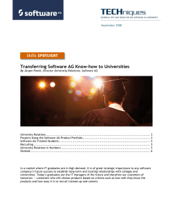
Proceedings of the 2005 International Conference on Simulation and Modeling
V. Kachitvichyanukul, U. Purintrapiban, P. Utayopas, eds.
ESTIMATION OF COST EFFICIENCY IN AUSTRALIAN UNIVERSITIES
Jocelyn Horne and Baiding Hu
Department of Economics
Macquarie University
Sydney, NSW 2109, AUSTRALIA
ABSTRACT
Various studies have been carried out on estimation of cost
functions for Australian universities, for example, Throsby
(1986) and Heaton and Throsby (1997, 1998), and Lloyd et
al (1993). While estimating a cost function with different
purposes, all of the studies have estimated an aggregate
cost function in the sense that the sampled institutions were
assumed to have the same cost function. The present study
differs from the previous studies in two aspects; first, it
employs the stochastic frontier analysis for the specification of a cost function for Australian universities, which
allows for the estimation of cost efficiency for each university. Secondly, a panel data set is utilised which enables
not only comparisons of cost efficiency between universities, but also hypothesis-testing of assumptions about university cost functions. The findings from the study contribute to the formulation of an equity-efficiency based
policy on university-financing.
1
INTRODUCTION
The incentive structure facing Australian universities has
changed in the past three decades. Over the past three decades, government funding per Australian university student
has fallen progressively and now stands at 40 percent of
total university revenue as compared to almost 100 percent
in the early 1970s. This factor alone has put pressure on
Australian universities to find new revenue sources and
contain costs. Australian universities also face increased
competition from technology developments and globalisation of education services. While recent reforms have
freed some resource constraints, especially on the revenue
side, the higher education system remains partially deregulated. Consequently, universities have new incentives to
use their resources more effectively.
The purpose of this paper is to quantify the efficiency
with which Australian universities utilise their existing resources. The study estimates the cost efficiency of Australian universities over the period 1995-2002 using stochastic frontier analysis. Its contribution to the literature is
primarily empirical: the paper is the first attempt to esti-
mate the cost efficiency of Australian universities and is
the first application of this methodology to measuring university efficiency. The findings also provide input into recent policy debate on the scope for accommodating recent
cutbacks in government funding to universities through increasing efficiency and other mechanisms.
There is no shortage of empirical studies of the cost
function of the higher education sector in Australia (see
Throsby, 1986; Lloyd, Morgan and Williams, 1993;
Heaton and Throsby, 1997). The methodology used in
these studies is to estimate either an aggregate output or
multiple output cost function. The main finding of this literature is to demonstrate the existence of internal economies-of-scale with minimum average and marginal costs of
around $11, 500 per EFTSU load in 1996 dollars. However, these studies assume that the cost function of each
university lies along the efficiency frontier. The empirical
methodology used in the present study provides a means of
testing the null hypothesis of optimal cost efficiency and
rejects it.
A relatively small empirical literature has examined
the technical efficiency (defined as the ability to minimise
input use for a given output) of universities; see Coelli
(1996) for Australia and McMillan and Datta (1998) for
Canada. Restriction to technical rather than cost efficiency
avoids the imposition of behavioural assumptions such as
cost minimisation although duality exists for both concepts
under certain assumptions about the production function
(see below). Both studies use the non-parametric methodology of data envelopment analysis (DEA) based upon linear programming techniques. An advantage of DEA
analysis is that it avoids potential problems involved in arbitrary specification of cost or production functions. But a
major shortcoming is its inability to provide statistical tests
of parameter estimates.
The empirical methodology of the present study uses
stochastic frontier analysis based upon panel data that enables testing of key hypotheses, including the null hypothesis of optimal efficiency as well as similarity of marginal costs of different teaching disciplines. Stochastic
frontier analysis has been used extensively in other areas of
economics such as airlines (Cornwell, et al, 1990) and the
Horne and Hu
manufacturing sector (Hay and Liu, 1997) but it is the first
time that the methodology has been applied to estimating
cost efficiency of universities.
Reform of the higher education sector in Australia has
been the subject of ongoing policy debate, especially in the
wake of Commonwealth funding cutbacks to universities
in a period of expanding student load (see King, 2001;
Chapman, 2001). The main thrust of reform efforts have
centred upon partial deregulation of fees with the introduction in 1989 of government subsidised HECS fees for domestic students and full-fees levied on other domestic and
foreign students. Reforms introduced in the 2003-4 Commonwealth Budget scheduled for implementation in 2005
extend the scope for universities to raise non-government
revenue in various ways: by widening the HECS bands, by
extending income-contingent loans to non-HECS students
and by increasing the proportion of fee-paying domestic
students from 25 to 33 percent (see Commonwealth of
Australia, 2003). But the reforms stop short of full fee deregulation and maintain centralised control of Commonwealth government funding of HECS-supported places.
At a policy level, the issue of university efficiency has
not been addressed in any systematic way but did receive
attention in the 2001 Senate Inquiry as well as policy discussion papers preceding the new reforms (see Commonwealth of Australia, 2001; Department of Education, Science and Training, 2002).
These documents give
conflicting views, reflecting the different definitions of efficiency and lack of empirical evidence. For example, at
the Senate Inquiry, policymakers argued that further efficiency gains might be achieved while universities felt that
this scope was exhausted.
Further understanding of the scope for efficiency gains
is of considerable interest for policymakers at a government and university level. Decisionmakers at both levels
have an interest in knowing whether government funding
to the sector (2.4 percent of Commonwealth expenditures
in 2003-4) is being used efficiently. But the issue extends
beyond this interest: if scope exists for further efficiency
gains, less adjustment is borne by other variables such as
student fees for meeting present and projected funding
gaps.
The major contribution of this study is to help fill this
gap in information on a key dimension of university performance, namely by estimating cost efficiency. Two
qualifications to the findings deserve mention at the outset,
the issue of quality and the factors behind difference in efficiency across universities. The perception of declining
quality of higher education dominates much of the debate
and affects the interpretation of any cost and efficiency estimates insofar as a relatively high ranking may reflect a
fall in the quality of education rather than a more effective
use of resources. We attempt to control for quality by introducing university-specific data on staff/student ratios as
a separate variable affecting university costs. But any in-
ferences that are drawn are subject to the problem of the
reliability of this measure in capturing quality changes.
A second issue concerns the factors that explain why
one university is relatively more efficient than another. The
methodology cannot answer this question: only the factors
behind individual university efficiency are estimated.
Nevertheless, the efficiency rankings are of potential use if
the allocation of government funding of teaching resources
were based upon performance criteria at a future date.
The remainder of the paper examines in more detail
the above issues. Section II discusses the issue of cost efficiency in the context of the debate on financing of Australian universities. Sections III and IV discuss the empirical
methodology used in the analysis, estimation results and
their interpretation. Section V presents the policy implications, main conclusions and directions for future research.
2
BACKGROUND AND ISSUES
The changes in financing sources of Australian universities over the sample period (1995-2002) are given in Table
1 and need to be viewed within the context of longer-term
trends in government financing of higher education (see
Marginson, 2001). Government expenditure on higher
education has halved as a percentage of GDP since its peak
of 1.5 in 1976-77. Over the same period, student numbers
increased by a multiple of three with a rise of one third recorded in the past decade.
Given the size of the government cutbacks, a key policy issue is how these changes are being accommodated at
a university level. A number of variables may bear the
burden of adjustment, including student numbers, revenue
and costs, financial solvency, quality of education and efficiency. The problem is that not all the variables are observable, in particular, the latter two. But based upon
available data, the picture that emerges is that most of the
adjustment has been on the revenue side and, especially in
terms of revenue composition.
The first adjustment mechanism at a university level is
a reduction in student load or numbers. The increase in total student numbers is spread across all universities and reflects the tying of Commonwealth funding through the
base operating grant to government funded places for domestic undergraduate students. At a university level, there
is little incentive to cut total student numbers and even
greater incentives to increase the share of full-fee paying
overseas students with consequent distortions across disciplines in favour of more business-oriented studies. The
data reflect this at an aggregate and university level: the
share of full-fee paying foreign students in total students
rose from 8 to almost 14 percent over the sample period.
A second adjustment mechanism is through changes in
revenues and costs. Average real revenue per full-time student rose from $ 7,535 to $11,615 from 1995 to 2002 but
average real costs per student remained stable at around
Horne and Hu
$15,000, leaving an average negative operating margin of
percent of average revenues in 2002 (Table 1). (In aggregate terms, there is a positive gap but, in any event, both
the average and aggregate pictures are deceptive because
the financing gap has moved in different directions for
universities.) However, universities are non-profit institutions and hence the concept and measurement of financial
criteria such as insolvency are not clearly defined. Most
universities have incentives to prevent a widening and
negative financing gap since the resulting debt buildup
constrains recurrent expenditures and thereby reduces their
flexibility of policy options.
A third mechanism is through a downward adjustment
in quality of teaching and other services. Trends in the
quality of higher education are difficult to measure. If
measured in terms of staff/student ratios, quality of higher
education has declined with an increased ratio from 15.3 in
1995 to 21.4 in 2002 with rises recorded for all universities
and in all disciplines. While anecdotal and survey data
support this interpretation, other measures provide conflicting evidence.
Assuming unchanged quality and a stable financing
gap, this leaves adjustment either from the composition of
revenues and costs or from efficiency. The data in Table 1
show that the share of Commonwealth grants in total revenue fell from 57.2 to 40.1 percent over 1995-2002 and was
offset partially by increased shares from full-fee paying
students and from subsidised HECS fees: non-HECS fee
share rose from 11.7 to 21.2 percent while that of HECS
rose from 12 to 15.8 percent with the remainder from other
items such as donations.
On the cost side, the composition remained fairly stable, reflecting the dominant share of wage costs: the share
of the staff wage bill fell from 63.6 percent in 1995 to 58.7
percent of total costs in 2002. But given the retrenchments
that have taken place in the past few years and the pressure
placed on universities from inadequate wage indexation to
allow for enterprise bargaining, there is little scope for significant further reduction.
This leaves one further option, increasing efficiency.
The concept and measurement of efficiency depend upon
the definition used (see below). The only available empirical evidence for Australia is based upon a multi-stage DEA
study by Coelli (1996) of technical efficiency for 36 universities in 1994. This study is, however, restricted to an
analysis of administrative efficiency and found a relatively
high average efficiency score of 0.8 against a benchmark
of unity for optimal efficiency. An empirical gap still exists on identifying changes in technical and cost efficiency
of teaching (and research) output and the scope for further
increases in efficiency. The issue of cost efficiency of
teaching output is addressed below.
Table 1: Revenues and expenditures of Australian universities, 1995-2002(in percent)
Revenues
1995
2002
Common. Govt.
57.2
40.1
grants
HECS
12.0
15.8
Fees and charges
11.7
21.2
Investment in4.0
1.8
come
State govt.
1.4
4.0
Other
13.8
17.1
100.0
100.0
Costs
Salaries
63.6
58.7
(academic)
(33.1)
(31.2)
Other
36.4
27.5
100.0
100.0
Memorandum
items
Average
real
7,535
11,614
revenue
per
EFTSU (in $)
Average real costs
15,069
15,677
per EFTSU (in $)
EFTSUs
544,146
626,749
Student/staff ratio
15.3
21.4
Source: DEST Selected Higher Education Statistics
3
METHODOLOGY
A number of different concepts of efficiency are discussed
in the literature and policy discussion, including technical,
cost and x-efficiency (see Kumbhakar and Lovell, 2000).
The focus of this study is upon cost efficiency of university
teaching resources: cost efficiency is defined as ability to
minimise costs for a given output vector and measured by
the ratio of minimum to observed cost. This concept differs
from technical efficiency, defined as the ability to minimise input use for a given output vector. Unlike cost efficiency, technical efficiency does not involve the imposition
of behavioural assumptions such as cost minimisation. Further, not all cost inefficiency need reflect technical efficiency. For example, an input vector may be technically
efficient but cost inefficient because of misallocation of inputs in terms of their relative prices.
In the following analysis, it is assumed that universities do attempt to minimise costs. This assumption may be
questioned on the grounds that universities are non-profit
institutions but, as noted above, the changing environment
has altered the incentive structure significantly and especially in the sample period.
The analytical framework of the present study is based
upon cost frontier analysis, which defines cost inefficiency
as the ratio of estimated cost frontier to observed cost
Horne and Hu
(Kumbhakar and Lovell, 2000). Figure 1 provides a simple illustration of the concept of cost inefficiency. Assuming that cost is determined by output, the cost inefficiency
for university A with output, Q , and cost, E A , is the ra-
Cost
Cost Frontier
tio of the distance CQ to the distance AQ , where C is
the minimum feasible cost or the cost frontier for producing output, Q . University A is more efficient than university B since the distance AC is shorter than distance
BC . As E A and E B are observable, estimation is required to “locate” C in order to calculate cost inefficiency.
Two approaches have been used to estimate a cost
frontier; stochastic frontier analysis (SFA) and data envelopment analysis (DEA) (for surveys, see Lovell, 1993;
Coelli et al (1998)). A major drawback of DEA is that it
does not allow hypothesis testing and assumes that every
observation unit operates under the same technology. In
the context of a panel data set, DEA virtually treats individual differences as fixed, ignoring the possibility of them
being random. As noted above, the Australian tertiary
education sector has undergone substantial changes during
the past decade, it is expected that the environment under
which a university operates may be different from university to university. Hence, it is advisable to subject such individual differences to a formal screening process. SFA
allows statistical hypotheses testing with regard to differences in university cost frontiers and is therefore chosen
over DEA for the present study.
Figure 1 assumes that universities A and B have an
identical cost frontier and there is single output for each of
them. For a more general analysis, it is conjectured that
universities have different cost frontiers, Ci , for given
EA
B
EB
A
C
Output
Q
Figure 1: An illustration of cost inefficiency
To take into account random shocks to the cost frontier, a stochastic component, ε i , is included in the cost
frontier, namely,
Ci = f (Yi , Pi , ε i )
(1)
Assuming a Cobb-Douglas functional form for the
f (•) and omitting Pi since factor prices (salaries of academic and non-academic staff) facing Australian universities are similar (Lloyd et al, 1993), equation (1) is written
as,
β
Ci = α i 0 Π Yij ij ε i
(2)
vectors of output and factor prices, Yi and Pi , respec-
where Yij is the jth element of Yi ,
α i 0 (intercept term)
i indexes the university. The Ci may be
represented by a function such as, Ci = f (Yi , Pi ) , where
f (•) characterises the underlying technology. The observed cost (nominal expenditure) for Yi is denoted by Ei
which equals Pi ' X i , where X i is a vector of input factors ( Pi and X i are conformably dimensioned).
and
tively, where
j
β ij s (university cost responsiveness to output change)
are parameters to be estimated. Equation (2) represents the
stochastic cost frontier for University i .
It
follows
by
definition
that
Ei = Pi ' X i ≥ Ci = f (Yi , Pi , ε i ) , which implies that cost
inefficiency has led to University
E −C
i to overspend by an
i (the difference between observed and
amount of i
estimated minimum cost).
Denote cost inefficiency by ui (≥ 0) and follow
Kumbhakar and Lovell (2000), the university expenditure
function is written as:
k
β
Ei = α i 0 Π qij ij ε i e ui
j =1
(3)
Horne and Hu
so that the cost efficiency (CE) can be measured by the ratio of Ci to Ei ,
CEi = exp(−ui ) .
(4)
Equation (3) can be rewritten in the following panel data
model specification,
ln Eit = ln α i 0 + ∑ β ij ln Yijt + vit + ui
j
or eit =
β i 0 + ∑ β ij yijt + vit + ui
(5)
j
where the lower case letters denote logarithms, subscript t
indexes time period and v is a white noise.
Estimation of the inefficiency component depends on
whether equation (5) is specified as a random or fixed effects model. A random effects model suggests that inefficiency differences between the universities are independent
of differences in university attributes, that is, the
independent of the
yijt
ui s, are
s. A fixed effects model, however,
y
u
is indicative of the i s being conditional on the ijt s.
Since the sample period spans only eight years, such a difference in model specification has a significant impact on
coefficient estimates (Hsiao, 2003, p. 37), which, in turn,
affect estimation of cost inefficiency. This gives rise to the
use of a specification test, such as Hausman (1978) to select one of the two model specifications.
Equation (5) indicates that cost inefficiency is different between universities but remains unchanged over time.
To overcome this limitation, the procedure proposed by
Cornwell et al (1990) is followed, which assumes that cost
inefficiency evolves over time according to
uit = δ i 0 + δ i1t + δ i 2t 2
where
δ i 0 , δ i1
and
δ i2
(6)
are cost-time variant university-
specific parameters to be estimated. There are two steps
involved in estimation of the δ i 0 , δ i1 and δ i 2 . In the first
step, equation (5) is either estimated by a least squares
dummy variable estimator if a fixed effects model specification is accepted, or by an estimated generalised least
squares estimator (EGLS) if a random effects model specification is accepted. In the second step, the estimated residuals in step one are regressed on t and t
estimates of the
δ i 0 , δ i1
and
δ i2 ,
2
to obtain the
denoted by δˆi 0 , δˆi1
and δˆi 2 . Thus, the estimates of the uit are computed by
uˆit = δˆi 0 + δˆi1t + δˆi 2t 2 , which are consistent estimators
when both the numbers of time period and panel units are
large (Greene, 1993).
To ensure the non-negativeness of the inefficiency
component (ruling out the possibility that observed cost
lies below minimum cost) requires a normalisation of the
uˆit s, which amounts to re-defining inefficiency as
uˆit − uˆmin t , where uˆ min t is the smallest uˆit for period t .
For example, suppose university A’s inefficiency at time t
is uˆ At = 0.8 and university B’s is uˆ Bt = −0.6 , then, the
uˆ min t will be uˆ Bt = −0.6 , namely, university B is the
most efficient university since its cost efficiency is 100%
( uˆ Bt − uˆ min t = −0.6 − ( −0.6) = 0 ), and using equation
(4) gives CE B = exp[−(uˆ Bt − uˆ min t )] = 1 ). The estimation procedure allows for time-varying costs and, hence,
the possibility that the most efficient university may alter
over the sample period.
4
ESTIMATION AND EMPIRICAL RESULTS
The data set for the present study are comprised of student,
staff and expenditure statistics for 36 Australian universities over the period 1995-2002, obtained from the Department of Education, Science and Training (DEST). The
student statistics enable a breakdown of student numbers
by field of study and mode of attendance. As noted above,
a number of studies have been conducted to estimate cost
functions for the Australian tertiary sector, including
Throsby (1986), Heaton and Throsby (1997, 1998), and
Lloyd et al (1993). A commonality among these studies is
that costs are assumed to be a function of student numbers
only since universities face similar factor prices (staff salaries are more or less identical across universities).
The cost determinant variables that appear on the right
hand side of equation (5) include the following: (a) postgraduate students (PG); (b) undergraduates (UG); (c) share
of science-engineering students (SE); (d) share of business
students (SB) and (e) share of other students (SO). To reflect the influence of teaching quality on cost formation, a
sixth variable, student-staff ratio (SR) is added. Staff data
by institution from 1995 to 1999 were not available and
therefore were estimated by applying staff growth rates at
the national level to existing staff numbers.
The six cost determinants listed above do not include
research output; research costs are measured by the difference between total expenditure and research expenditure.
Data on research costs are not published either by DEST or
Australian Bureau of Statistics (ABS). However, shares of
research income by institution from 1995 to 1999 and total
Horne and Hu
research expenditures by all the universities from 1995 to
2002 are available at DEST and ABS, respectively. It is
assumed that the share of research income at an institution
is positively correlated with its share of research expenditure. Thus, research expenditure for each university is estimated by applying its share of research income (expenditure) to the total research expenditure.
The estimated random effects panel data model is as
follows,
eit = β i 0 + β i1 ln PG + β i 2 ln UG + β i 3 ln SE +
β i 4 ln SB + β i 5 ln SO +
β i 6 ln SR + vit + ui
(7)
where i =1 to 36, t =1995 to 2002.
The first step in the analysis is to test if each of the
universities has a different cost function. This amounts to
conducting an F-test for the following hypotheses.
H 0 : β1,0 = ⋅ ⋅ ⋅ = β 36,0 ; β1,k = ⋅ ⋅ ⋅ = β 36,k ; k = 1 to 6
H1 : at least one of the βs is different.
The F-test indicates that the above null hypothesis
should be rejected, which vindicates use of a panel data
modelling approach. Further F-tests are conducted to find
out whether the universities share the same intercept or the
same slope coefficients. Such tests reveal that the universities share the same slope coefficient, namely,
β1,k = ⋅ ⋅ ⋅ = β 36,k = β k ; k = 1 to 6 . This implies that the
universities have the identical “technology” to produce
students of various fields in terms of cost elasticity of student. However, the universities do have a different intercept coefficient, namely, the null hypothesis
H 0 : β1,0 = ⋅ ⋅ ⋅ = β 36,0 is rejected. This is followed by a
Hausman test, which gives rise to a random effects specification for the panel model. This implies that university
cost inefficiency is exogenous to student numbers. The estimated model (by the EGLS procedure) is given below
with the asymptotic t-ratios in the parentheses.
eˆit = 7.9291+ 0.1213 ln PGit + 0.4785 ln UGit + 0.6351 ln SEit +
(11.1485 )
( 2.9080 )
( 7.0404 )
( 3.3625 )
(8)
0.3674 ln SBit + 0.3747 ln SOit − 0.0721 ln SRit
( 2.9215 )
(1.8280 )
( −2.6375 )
R 2 = 0.49 F = 45.66 Hausman test = 0.0001
The estimation procedure has taken into account potential
cross-sectional heteroskedasticity but ignored the possible
existence of autocorrelation. To address potential autocor-
relation issues will substantially complicate the estimation
process as the efficiency of the model coefficient estimates
depends on finding a consistent estimator of the autocorrelation coefficient. This, in turn, requires the number of
time periods being large, which is not the case in the present study (Hsiao, 2003, p57). Thus, autocorrelation is ignored.
The t-ratio of the variable, ln SOit , is insignificant at
a 5 percent level, which suggests that students of fields
other than science/engineering and business have an insignificant impact on university cost, ceteris paribus. All
other independent variables, including the quality variable
are significant at a 5 percent level; each coefficient measures the cost elasticity response. For example, the estimates show that a 10 percent increase in undergraduates
increases costs for all universities by the same amount, almost 5 percent. Increasing the relative share of business
students has a smaller effect on costs compared to nonbusiness students. The elasticity of university costs in response to the proportion of science to business students is
almost double that of business students alone while the
cost elasticity of undergraduates is four times that of postgraduates. Quality of teaching has a small but significant
negative impact on costs: a rise in the student/staff ratio of
1 percent reduces costs by less than 0.1 percent.
The coefficients in equation (8), which are cost elasticites of student, are not directly comparable with those in
the previously estimated cost functions for Australian universities (Heaton and Throsby, 1997 and Lloyd et al, 1993)
since the coefficients in the latter studies are marginal costs
of student. Further, a constant cost elasticity, which is the
case in the present study, implies a variable marginal cost.
However, it is worthwhile to note that the cost elasticity for
postgraduate students was found to be smaller than that for
undergraduate students in the present study. Lack of
knowledge of various student proportions in 1991 and
1994, the elasticity estimates in equation (8) would be consistent with the previous studies which point to the marginal cost of postgraduate students being higher than that
of undergraduate students if the proportions of undergraduate students in the years were high enough.
Residuals from model specified by equation (8) are
used as the dependent variable for the auxiliary regression
outlined in Section III for estimation of time-varying cost
inefficiency. Table 2 contains estimates of cost efficiency
calculated using equation (4) for 36 Australian universities:
efficiency rankings are presented in Table 3.
In interpreting the results, it is recalled that the normalisation procedure estimates university efficiency relative to the most efficient university (benchmark) in a given
year. The benchmark is endogenously determined and
hence, can change over time as shown in the Table. It appears that the non-Go8 universities have dominated the top
10 places in terms of cost efficiency. Only the University
of Adelaide and the University of Western Australia are in
Horne and Hu
the top 10 throughout the sample period. The most efficient
universities are the University of Ballarat and Flinders
University with the latter outpacing the former in recent
years. The least efficient in every year is ANU. There is
no discernible pattern of an increase in cost efficiency (increase in ratio) over time. Further, the results suggest scope
for increasing cost efficiency: in 2002, the average cost efficiency is below 0.5.
5.
POLICY IMPLICATIONS AND CONCLUSIONS
Three main policy issues arise from the empirical findings:
the scope for efficiency adjustment in response to government funding cutbacks, the use of efficiency rankings as
performance criteria for government funding of teaching
resources and measures to increase relative efficiency.
An earlier study by Heaton and Throsby (1997) examined the policy implications of estimated university cost
functions of Australian universities, including the effects of
cuts in government funding. Their study demonstrated that,
barring other adjustment mechanisms such as efficiency
and assuming unchanged fees and quality, costs can be reduced through a redistribution of students from universities
operating above minimum scale. The difficulty with this
reform is that there are disincentives for universities to reduce student numbers under current as well as proposed
Commonwealth funding arrangements that tie funds to a
specified number of government supported undergraduate
places in particular course disciplines.
The main finding of this study is that universities are
not operating efficiently, as measured by cost efficiency
and in relative terms. In terms of movement towards relatively greater efficiency, not all universities can improve
their rankings since it is a zero sum game. But on average
the size of efficiency gaps is below 0.5 suggesting scope
for further gains in cost efficiency. (The normalisation procedure converts cost efficiency residuals into the difference
between the benchmark university and that of a specific
university and hence, any dollar transformation of the efficiency rankings has little meaning.)
A second issue concerns the potential policy use
of the efficiency rankings in allocating government funding of teaching resources. Unlike research funding which is
based upon a competitive set of performance criteria, the
current system of block operating grants and its successor
(Commonwealth Grant Scheme) are input based with educational and other performance criteria having little or no
effect on government funding for teaching. Although each
university has an incentive to manage its costs effectively,
there is no information on how they compare to others or
rewards for relative efficiency. The efficiency rankings
provide quantitative measurement of one dimension of
university output that might be used together with other
criteria such as undergraduate degree completions and
quality control benchmarks.
Table 2: Efficiency estimates (ratio of minimum feasible
cost to actual cost)
Year 1995 1996 1997 1998 1999 2000 2001 2002
ACU 0.58 0.58 0.59 0.60 0.58 0.52 0.46 0.40
CQU 0.85 0.80 0.75 0.71 0.65 0.56 0.47 0.39
CSU 0.69 0.66 0.64 0.65 0.64 0.60 0.56 0.53
CUT 0.58 0.55 0.52 0.51 0.48 0.43 0.38 0.33
DU
0.56 0.55 0.54 0.53 0.50 0.44 0.38 0.31
ECU 0.57 0.55 0.54 0.55 0.53 0.49 0.45 0.40
GU
0.61 0.58 0.55 0.54 0.51 0.45 0.39 0.34
JCU 0.58 0.60 0.61 0.63 0.62 0.57 0.50 0.44
LTU 0.55 0.57 0.58 0.59 0.56 0.49 0.41 0.33
MQU 0.64 0.66 0.67 0.67 0.63 0.54 0.45 0.35
MOU 0.52 0.50 0.49 0.48 0.45 0.40 0.35 0.30
MDU 0.87 0.85 0.82 0.81 0.77 0.68 0.59 0.50
NTU 0.80 0.86 0.89 0.92 0.87 0.76 0.63 0.49
QUT 0.58 0.56 0.54 0.54 0.52 0.47 0.43 0.39
RMIT 0.54 0.56 0.57 0.57 0.53 0.46 0.37 0.29
SCU 0.96 0.96 0.94 0.94 0.89 0.79 0.69 0.57
SUT 0.81 0.87 0.89 0.89 0.81 0.66 0.50 0.35
ANU 0.19 0.20 0.21 0.22 0.22 0.20 0.17 0.15
FU
0.90 0.90 0.91 0.97 1.00 1.00 1.00 1.00
UAD 1.00 0.87 0.79 0.76 0.72 0.68 0.65 0.63
UML 0.56 0.60 0.62 0.64 0.61 0.53 0.44 0.35
UNE 0.56 0.57 0.58 0.60 0.58 0.52 0.46 0.39
UNSW0.47 0.50 0.52 0.55 0.55 0.50 0.45 0.38
UNC 0.68 0.69 0.70 0.71 0.67 0.60 0.51 0.42
UQ
0.76 0.72 0.68 0.65 0.58 0.49 0.41 0.32
USD 0.36 0.41 0.45 0.49 0.49 0.45 0.39 0.32
UWA 0.92 0.78 0.69 0.66 0.63 0.59 0.56 0.55
UB
0.98 1.00 1.00 1.00 0.93 0.80 0.66 0.51
UC
0.85 0.83 0.81 0.81 0.77 0.70 0.62 0.54
USA 0.60 0.58 0.57 0.59 0.57 0.54 0.50 0.45
USQ 0.91 0.82 0.77 0.77 0.75 0.71 0.69 0.67
UTAS 0.77 0.77 0.77 0.78 0.75 0.67 0.59 0.50
UTS 0.61 0.62 0.63 0.64 0.61 0.55 0.48 0.40
UWS 0.55 0.55 0.54 0.55 0.54 0.49 0.45 0.39
UW 0.74 0.72 0.71 0.72 0.71 0.67 0.62 0.58
VUT 0.67 0.69 0.69 0.69 0.64 0.56 0.46 0.36
A third issue follows from the second: if the rankings
are to be of operational use, what measures are within university control to improve relative efficiency, especially in
relation to the findings of scale effects of cost studies?
Statistical support for the random effects model implies
that student numbers are exogenous to efficiency. However, as noted at the outset, the SFA methodology cannot
explain the factors behind the rankings and, hence, how a
university can improve its relative position. For example,
rises in the staff student ratio has a small and significant
negative effect on university costs but an across the board
reduction in this ratio has little effect on efficiency rankings.
Horne and Hu
Table 3: Rankings of universities by cost efficiency (most
efficient to least efficient).
1995
UAD
UB
SCU
UWA
USQ
FU
MDU
CQU
UC
SUT
NTU
UTAS
UQ
UW
CSU
UNC
VUT
MQU
UTS
GU
USA
QUT
CUT
JCU
ACU
ECU
DU
UML
UNE
UWS
LTU
RMIT
MOU
UNSW
USD
ANU
1996
UB
SCU
FU
SUT
UAD
NTU
MDU
UC
USQ
CQU
UWA
UTAS
UQ
UW
UNC
VUT
MQU
CSU
UTS
UML
JCU
ACU
USA
GU
UNE
LTU
RMIT
QUT
ECU
DU
UWS
CUT
MOU
UNSW
USD
ANU
1997
UB
SCU
FU
SUT
NTU
MDU
UC
UAD
USQ
UTAS
CQU
UW
UNC
UWA
VUT
UQ
MQU
CSU
UTS
UML
JCU
ACU
LTU
UNE
USA
RMIT
GU
UWS
ECU
DU
QUT
UNSW
CUT
MOU
USD
ANU
1998
UB
FU
SCU
NTU
SUT
MDU
UC
UTAS
USQ
UAD
UW
CQU
UNC
VUT
MQU
UWA
CSU
UQ
UML
UTS
JCU
ACU
UNE
LTU
USA
RMIT
UWS
UNSW
ECU
GU
QUT
DU
CUT
USD
MOU
ANU
1999
FU
UB
SCU
NTU
SUT
UC
MDU
UTAS
USQ
UAD
UW
UNC
CQU
VUT
CSU
MQU
UWA
JCU
UTS
UML
UQ
ACU
UNE
USA
LTU
UNSW
UWS
RMIT
ECU
QUT
GU
DU
USD
CUT
MOU
ANU
2000
2001
2002
FU
FU
FU
UB
USQ USQ
SCU
SCU UAD
NTU
UB
UW
USQ
UAD SCU
UC
NTU UWA
MDU
UC
UC
UAD
UW
CSU
UTAS UTAS
UB
UW
MDU UTAS
SUT
CSU MDU
CSU
UWA NTU
UNC
UNC USA
UWA
JCU
JCU
JCU
SUT UNC
CQU
USA ECU
VUT
UTS
UTS
UTS
CQU ACU
MQU
ACU UWS
USA
UNE UNE
UML
VUT CQU
ACU UNSW QUT
UNE
ECU UNSW
UNSW UWS VUT
UWS
MQU SUT
UQ
UML MQU
LTU
QUT UML
ECU
LTU
GU
QUT
UQ
LTU
RMIT
USD CUT
USD
GU
UQ
GU
DU
USD
DU
CUT
DU
CUT
RMIT MOU
MOU MOU RMIT
ANU
ANU ANU
The main conclusion reached is that the hypothesis that universities are operating at minimum cost efficiency is rejected over the sample period 1995-2002. The
period encompasses the peak of the debate on reform of
higher education, including conflicting views on this dimension of university performance. The main direction of
further research is to extend the model to include factors
that explain the efficiency rankings and thereby provide
scope for universities to strengthen their absolute and relative performance over time.
REFERENCES
Chapman, B. 2001. Australian Higher Education Financing: Issues for Reform. The Australian Economic Review 34: 195-204.
Cornwell, C, P. Schmidt and R.C. Sickles. 1990. Production Frontiers With Cross-Sectional And Time-Series
Variation In Efficiency Levels. Journal of Econometrics 46: 185-200.
Coelli, T.J. 1996. Assessing the Performance of Australian
Universities Using Data Envelopment Analysis.
Mimeo, Centre for Efficiency and Productivity Analysis University of New England.
Coelli, T.J, D.S.P. Rao and G. Battese. 1998. An Introduction to Efficiency and Productivity Analysis. Kluwer
Academic Publishers, Boston.
Commonwealth of Australia. 2003. Our Universities Backing Australia’s Future. www.backingaustraliasfuture.
gov.au
Department of Education, Science and Training, Selected
Higher Education Statistics. DEST, Canberra,
www.dest.gov.au
________(2002) Setting Firm Foundations Financing Australian Higher Education. DEST, Canberra,
www.dest.gov.au,
Greene, W. 1993. The Econometric Approach to Efficiency Analysis, in H.O. Fried, C.A.K. Lovell and S.
Schmidt (eds.), The Measurement of Productivity Efficiency: Techniques and Applications. Oxford University Press, New York: 69-119.
Hay, D. and G.S. Liu. 1997. The Efficiency of Firms: What
Difference Does Competition Make? The Economic
Journal. 107: 597-617.
Hausman, J.A. 1978. Specification Tests in Econometrics.
Econometrica, 46: 1251-1271.
Heaton , C and D. Throsby. 1997. Cost Functions for Australian Universities: A Survey of Results with Implications for Policy. Centre for Economic Policy Research Discussion Papers, No. 360, February.
Hsiao, C. 2003. Analysis of Panel Data, Cambridge University Press, Cambridge.
King, S. 2001. The Funding of Higher Education in Australia: Overview and Alternatives. The Australian Economic Review, 34: 190-194.
Kumbhakar, S and C. Knox Lovell. 2000. Stochastic
Frontier Analysis, Cambridge University Press, Cambridge.
Lloyd, P, M. Morgan and R. Williams. 1993. Amalgamation of Universities: Are There Economies of Scale or
Scope? Applied Economics, 25: 1081-1092.
Marginson, S. 2001. Trends in the Funding of Australian
Higher Education. The Australian Economic Review,
43: 205-215.
McMillan, M and D. Datta. 1998. The Relative Efficiencies of Canadian Universities: A DEA Perspective.
Canadian Public Policy, XXIV: 485-511.
Throsby, D. 1986. Cost Functions for Australian Universities. Australian Economic Papers, 25:175-92.
Senate Employment, Workplace Relations, Small business
and Education Reference Committee. 2001. Universi-
Horne and Hu
ties in Crisis, www.aph.gov.au/senate/committeee/
et_ctte/public%20uni/report/index.htm
Appendix A : UNVERSITY ABBREVIATIONS
ACU Australian Catholic University
CQU Central Queensland University
CSU Charles Sturt University
CUT Curtin University of Technology
DU
Deakin University
ECU Edith Cowan University
GU
Griffith University
JCU James Cook University
LTU La Trobe University
MQU Macquarie University
MOU Monash University
MDU Murdoch University
NTU Northern Territory University
QUT Queensland University of Technology
RMIT RMIT University
SCU Southern Cross University
SUT Swinburne University of Technology
ANU The Australian National University
FU
The Flinders University of South Australia
UAD The University of Adelaide
UML The University of Melbourne
UNE The University of New England
UNSW The University of New South Wales
UNC The University of Newcastle
UQ
The University of Queensland
USD The University of Sydney
UWA The University of Western Australia
UB
University of Ballarat
UC
University of Canberra
USA University of South Australia
USQ University of Southern Queensland
UTAS University of Tasmania
UTS University of Technology, Sydney
UWS University of Western Sydney
UW University of Wollongong
VUT Victoria University