
A Courseware Sample Telecommunications Communications Technologies
Telecommunications Communications Technologies Courseware Sample 85031-F0 A TELECOMMUNICATIONS COMMUNICATIONS TECHNOLOGIES COURSEWARE SAMPLE by the Staff of Lab-Volt Ltd. Copyright © 2009 Lab-Volt Ltd. All rights reserved. No part of this publication may be reproduced, in any form or by any means, without the prior written permission of Lab-Volt Ltd. Printed in Canada April 2009 Table of Contents Introduction Courseware Outline Spread Spectrum (DSSS / FHSS / CDMA) Sample Exercise Extracted from Spread Spectrum (DSSS / FHSS / CDMA) Exercise 1-2 Principles of Code-Division Multiple Access (CDMA) Other Sample Extracted from Spread Spectrum (DSSS / FHSS / CDMA) Unit Test 1 Direct-Sequence Spread Spectrum Instructor Guide Sample Exercise Extracted from Spread Spectrum (DSSS / FHSS / CDMA) Exercise 1-2 Principles of Code-Division Multiple Access (CDMA) Bibliography III IV Introduction Digital communication offers so many advantages over analog communication that the majority of today's communications systems are digital. Unlike analog communication systems, digital systems do not require accurate recovery of the transmitted waveform at the receiver end. Instead, the receiver periodically detects which waveform is being transmitted, among a limited number of possible waveforms, and maps the detected waveform back to the data it represents. This allows extremely low error rates, even when the signal has been corrupted by noise. The digital circuits are often implemented using application specific integrated circuits (ASIC) and field-programmable gate arrays (FPGA). Although this "system-on-a-chip" approach is very effective for commercial and military applications, the resulting systems do not allow access to internal signals and data and are therefore poorly suited for educational use. It is for this reason that Lab-Volt designed the Communications Technologies Training System. The Lab-Volt Communications Technologies Training System, Model 8087, is a state-of-the-art communications training system. Specially designed for hands-on training, it facilitates the study of many different types of digital modulation/demodulation technologies such as PAM, PWM, PPM, PCM, Delta Modulation, ASK, FSK, and BPSK as well as spectrally efficient technologies such as QPSK, QAM, and ADSL. The system also enables the study of direct-sequence and frequency-hopping spread spectrum (DSSS and FHSS), two key technologies used in modern wireless communication systems (CDMA cellular-telephony networks, Global Positioning System, Bluetooth interface for wireless connectivity, etc.) to implement code-division multiple access (CDMA), improve interference rejection, minimize interference with other systems, etc. The system is designed to reflect the standards commonly used in modern communications systems. Unlike conventional, hardware-based training systems that use a variety of physical modules to implement different technologies and instruments, the Communications Technologies Training System is based on a Reconfigurable Training Module (RTM) and the Lab-Volt Communications Technologies (LVCT) software, providing tremendous flexibility at a reduced cost. Each of the communications technologies to be studied is provided as an application that can be selected from a menu. Once loaded into the LVCT software, the selected application configures the RTM to implement the communications technology, and provides a specially designed user interface for the student. The LVCT software provides settings for full user control over the operating parameters of each communications technology application. Functional block diagrams for the circuits involved are shown on screen. The digital or analog signals at various points in the circuits can be viewed and analyzed using the virtual instruments included in the software. In addition, some of these signals are made available at physical connectors on the RTM and can be displayed and measured using conventional instruments. The courseware for the Communications Technologies Training System consists of a series of student manuals covering the different technologies as well as instructor guides that provide the answers to procedure step questions and to review questions. The Communications Technologies Training System and the accompanying courseware provide a complete study program for these key information-age technologies. V VI Courseware Outline SPREAD SPECTRUM (DSSS / FHSS / CDMA) Unit 1 Direct-Sequence Spread Spectrum Spread-Spectrum Technology Basics. Spread-Spectrum ModulationTechniques. Process Gain of Spread Spectrum Systems. Ex. 1-1 DSSS Signal Generation and Demodulation Generating DSSS Signals. Demodulating DSSS Signals Using In-Line Correlation. Demodulating DSSS Signals Using Heterodyne Correlation. DSSS Transmitter Using All Digital Modulation. Spreading Factor. DSSS Receiver (All-Digital-Modulation Implementation). Bandwidth Limitation and Pulse Shaping in DSSS Systems. The Lab-Volt Direct-Sequence Spread Spectrum (DSSS) Application. Ex. 1-2 Principles of Code-Division Multiple Access (CDMA) Multiple Access in Wireless Communication Systems. Implementing CDMA Using DSSS Technology. Pseudo-Random Code Sequences Used in DSSS Applications. Autocorrelation and Cross-Correlation Functions of Code Sequences. The Gold Code Generator. CDMA Cellular-Telephony Networks. The Near-Far Problem. Ex. 1-3 Process Gain and Interference Rejection in DSSS Wireless Communication Systems Process Gain in DSSS Communication Systems. Rejection of Fixed-Frequency Interference in DSSS Communication Systems. Process Gain in the Global Positioning System (GPS). Interference in CDMA Wireless Communication Systems Using DSSS Technology. Ex. 1-4 Synchronization – Acquisition and Tracking Introduction to Synchronization. Synchronization Acquisition Techniques. Synchronization Acquisition Technique Used in the Lab-Volt DSSS Application. Synchronization Tracking Using a Delay-Lock Loop (DLL). Ex. 1-5 Voice Transmission in CDMA Wireless Communication Systems Transmission Speed Versus Maximum Number of Users. Using Voice Encoders to Reduce Voice Data Rates. Introduction to Voice Encoding. Generic Block Diagrams of Voice Encoders and Decoders. FEC in Vocoders. Overview of the Lab-Volt CDMA Application. VII Courseware Outline SPREAD SPECTRUM (DSSS / FHSS / CDMA) Unit 2 Frequency-Hopping Spread Spectrum Introduction to Frequency-Hopping Spread Spectrum. Ex. 2-1 FHSS Signal Generation A Simple FHSS Transmitter. Generic Block Diagram of an FHSS Transmitter. Direct Generation of an FSK/FHSS Signal. Effect of Digital Modulation on the Transmitted Signal Frequency Spectrum. PN Codes Used in FHSS Applications. Bandwidth Limitation of the FHSS Signal. Transmitters in the Lab-Volt FHSS Application. Ex. 2-2 FHSS Signal Demodulation Introduction to FHSS Signal Demodulation. Generic Architecture of FHSS Receivers. The Receiver in the Lab Volt FHSS Application. Ex. 2-3 Interference Rejection in FHSS Wireless Communication Systems Interference in Communication Systems. Rejection of Fixed-Frequency Interference in FHSS Communication Systems. Error Probability in FHSS Communication Systems Submitted to Fixed-Frequency Interference. Effect of Fixed-Frequency Interference on Binary FSK Signals. Error Probability in FSK/FHSS Communication Systems Submitted to Fixed-Frequency Interference. Introduction to Fast Frequency Hopping. Introduction to CDMA Using FHSS Technology. Interference and Error Probability in CDMA Wireless Communication Systems Using FHSS Technology. Reducing the Error Probability in CDMA Wireless Communication Systems Using Fast Frequency Hopping. Use of FEC in FHSS Wireless Communication Systems. Ex. 2-4 Synchronization – Acquisition and Tracking Introduction to Synchronization. Synchronization Acquisition in FHSS Receivers Using the Serial-Search Technique. Synchronization Tracking in FHSS Receivers Using the Split-Bit Tracking Technique. Appendix A VIII Glossary of New Terms Sample Exercise Extracted from Spread Spectrum (DSSS / FHSS / CDMA) Exercise 1-2 Principles of Code-Division Multiple Access (CDMA) EXERCISE OBJECTIVE When you have completed this exercise, you will understand what multiple access is in wireless communication systems. You will be familiar with the principles of code-division multiple access (CDMA). You will understand how CDMA can be implemented using direct-sequence spread spectrum (DSSS) technology. You will be familiar with the autocorrelation and cross-correlation functions related to pseudo-random code sequences. You will learn how a large number of pseudo-random code sequences can be produced using a Gold code generator. You will be introduced to the use of CDMA in cellular telephony networks. You will be familiar with the near-far problem. DISCUSSION OUTLINE The Discussion of this exercise covers the following points: DISCUSSION Multiple Access in Wireless Communication Systems Implementing CDMA Using DSSS Technology Pseudo-Random Code Sequences Used in DSSS Applications Autocorrelation and Cross-Correlation Functions of Code Sequences The Gold Code Generator CDMA Cellular-Telephony Networks The Near-Far Problem Multiple Access in Wireless Communication Systems Most wireless communication systems used today are of the multiuser type. A multiuser system is able to share its total communication capability among multiple users in such a way that every user can transmit and receive information independently of the other users with minimal interference between the users. The property of a wireless system to share its communication capability between multiple users is generally referred to as multiple access. Various multiple access schemes have been devised for wireless communication systems. One of the first multiple access schemes developed uses frequency as a means of discriminating between the various users of the system. This multiple access scheme is called frequency-division multiple access (FDMA). FDMA separates the total bandwidth (WT) allocated to the system into several segments of equal width (WK), each segment being continuously available to a single user for both information transmission and reception. An example of a system in which the total bandwidth WT is separated between K users is shown in Figure 1-37. This leads to frequency segments having a bandwidth WK equal to WT/K. The higher the number of users K, the lower the bandwidth WK allocated to each user, and the lower the rate at which each user can transmit information (data). Therefore, the minimum information transmission rate (data rate) required imposes a limit on the maximum number of users which an FDMA system can support. Spread Spectrum (DSSS/FHSS/CDMA) 55 Ex. 1-2 – Principles of Code-Division Multiple Access (CDMA) Discussion Figure 1-37. Frequency-division multiple access (FDMA). To ensure correct separation of the various users in FDMA-based systems, one must be able to isolate the signal of any particular user from those of the other users. This is usually accomplished using bandpass filters. However, due to practical limitations of filters, guard bands (unused frequencies) are usually inserted between the various frequency segments. This prevents the spectra of adjacent user signals from overlapping each other, and thus, preserves the orthogonality (independence) of the user signals. Time is another parameter that is used as a means of discriminating users in a multiple-access wireless system. In this case, the multiple access scheme is called time-division multiple access (TDMA). TDMA separates the total time resource (TT) into several segments of equal duration (TK), in each of which the total frequency bandwidth (WT) allocated to the system is available to a single user. An example of a system in which the total time resource TT is separated between K users is shown in Figure 1-38. The higher the number of users K, the lower the time segment TK allocated to each user, and the lower the rate at which each user can transmit information (data). Therefore, the minimum information transmission rate (data rate) required imposes a limit on the maximum number of users which a TDMA system can support. Figure 1-38. Time-division multiple access (TDMA). To ensure correct separation of the various users in TDMA-based systems, strict time synchronization is required to allow the signal of any particular user to be 56 Spread Spectrum (DSSS/FHSS/CDMA) Ex. 1-2 – Principles of Code-Division Multiple Access (CDMA) Discussion correctly recovered. Guard intervals where no user signal is transmitted are sometimes inserted between the time segments to help preserve the orthogonality of the user signals. Another multiple access scheme that is widely used in modern wireless communication systems is called code-division multiple access (CDMA). CDMA uses binary codes to separate (identify) the signals of the various users instead of separating the total frequency bandwidth (WT) allocated to the system or the total time resource (TT) among the various users. As a result, in a CDMA system, both the total bandwidth allocated to the system and total time resource are available to each user. Figure 1-39 shows the allocation of the bandwidth and time resources in CDMA, FDMA, and TDMA systems. Figure 1-39. Allocation of the bandwidth and time resources in CDMA, FDMA, and TDMA systems. To ensure correct discrimination of the various users in CDMA-based systems, the codes used must be carefully selected so as to be as close as possible to perfect orthogonality (in this case, mathematical). Figure 1-39 suggests that the information transmission rate (data rate) that can be achieved for each user with CDMA is much higher than with either FDMA or Spread Spectrum (DSSS/FHSS/CDMA) 57 Ex. 1-2 – Principles of Code-Division Multiple Access (CDMA) Discussion TDMA since both the total frequency bandwidth (WT) allocated to the system and the total time resource (TT) are made available to each user. Figure 1-39 also suggests that the number of users is unlimited when CDMA is used. However, this is not the case in actual applications for reasons that will be explained later in this discussion. The total information transmission rate that can be achieved in a CDMA-based system (system throughput) is approximately the same as that which can be obtained with either an FDMA-based system or a TDMA-based system. Nevertheless, CDMA has several unique advantages over FDMA and TDMA, as will be explored later in this unit. Implementing CDMA Using DSSS Technology Codes (e.g., Walsh codes) other than pseudo-random code sequences can also be used in DSSS applications to spread the bandwidth of the information signal to be transmitted. Study of these codes, however, is beyond the scope of this manual. Code-division multiple access (CDMA) is commonly implemented using directsequence spread spectrum (DSSS) technology in actual applications. In a DSSS system, the information signal (data) to be transmitted is mixed with a pseudorandom code sequence to spread the bandwidth of the transmitted signal. At reception, the exact same code sequence is used to reduce the bandwidth of the received spread spectrum signal back to that of the information signal transmitted. The information (data) transmitted is then recovered. Any other signal that does not have the signature applied to the transmitted spread spectrum signal by the pseudo-random code sequence used is rejected at reception. Therefore, the pseudo-random code sequence used in the bandwidth spreading and reduction is a means of identifying a transmitted signal. A set of spread spectrum signals having recognizable signatures can be produced by using different pseudo-random code sequences. Assigning a code sequence to a user provides an efficient means of identifying the spread spectrum signal related to each user (user signal), and thus, allows discrimination of the various user signals. This is exactly what is required to implement a CDMA system. Figure 1-40 shows a simplified block diagram of a K-user CDMA wireless communication system using DSSS technology to separate the signals from the various users. In this system, K different pseudo-random code sequences, selected to be as orthogonal as possible with respect to each other, are produced. Each DSSS transmitter uses one of these K different pseudo-random code sequences to spread the bandwidth of a user information signal, i.e., to produce a recognizable spread spectrum signal. All the spread spectrum signals produced are centered on the same frequency and have the same bandwidth. The DSSS receiver can demodulate (correlate) any of the spread spectrum signals transmitted, and thus, recover the information transmitted by any one of the K users. The spread spectrum signal that is effectively demodulated depends on which one of the K pseudo-random code sequences is used in the DSSS receiver. 58 Spread Spectrum (DSSS/FHSS/CDMA) Ex. 1-2 – Principles of Code-Division Multiple Access (CDMA) Discussion Figure 1-40. Simplified diagram of a K-user CDMA wireless communication system implemented using DSSS technology. A DSSS transmitter greatly spreads the bandwidth of the information signal to be transmitted, thereby resulting in a spread spectrum signal with a low PSD. This generally results in a low S/N ratio at the DSSS receiver input. Fortunately, the bandwidth spreading and reduction performed in a DSSS system provides a process gain that improves the S/N ratio (after correlation in the DSSS receiver), helping to correctly recover the user information even if the spread spectrum signal PSD is low. This process gain is proportional to the spreading factor. When many spread spectrum signals are transmitted in the same bandwidth as is the case in the CDMA wireless communication system illustrated in Figure 140, this generally leads to a low S/N ratio at the DSSS receiver input. This is because each spread spectrum signal transmitted acts as a source of interference to the other signals. Therefore, the higher the number K of users in a CDMA wireless communication system, the lower the S/N ratio at the DSSS receiver input. To counterbalance this effect, the spreading factor can be made proportional to the number of users. Therefore, the higher the number of users, the higher the spreading factor, the higher the process gain, and the better the S/N ratio (after correlation in the DSSS receiver). Increasing the spreading factor, however, decreases the data rate. Therefore, increasing the number of users decreases the information rate for each user. This explains why the throughput in CDMA based communication systems is not usually significantly higher than that achieved in FDMA and TDMA communication systems. Pseudo-Random Code Sequences Used in DSSS Applications A pseudo-random code sequence is required in a DSSS system to achieve bandwidth spreading at the transmitter and the corresponding bandwidth reduction at the receiver. A pseudo-random code sequence has characteristics that are very close to those of purely-random binary data streams, but is totally Spread Spectrum (DSSS/FHSS/CDMA) 59 Ex. 1-2 – Principles of Code-Division Multiple Access (CDMA) Discussion predictable and reproducible. In fact, a pseudo-random code sequence is a predetermined sequence of ones and zeroes that is periodic (repeats itself over and over). The predictability and reproducibility of pseudo-random code sequences is essential in DSSS systems because an exact copy of the code sequence used in the transmitter to achieve spectrum spreading must be generated in the receiver to reduce the bandwidth of the received spread spectrum signal back to that of the information signal transmitted. A register output stage that is used to produce the feedback signal in an LFSR generator is commonly referred to as a tap. A pseudo-random code sequence can be produced using a linear-feedback, shift-register generator (LFSR generator). This type of generator consists of a shift register whose input is fed by a signal formed by combining the outputs of different stages of the shift register through modulo-2 adders. The combination of register output stages that is selected to produce the feedback signal determines the length of the pseudo-random code sequence and the arrangement of the ones and zeroes in the code sequence. The maximum sequence length (MSL) that can be obtained using an LFSR generator is determined by the following equation: MSL = 2 n − 1 (1-1) Where n is the number of stages in the shift register. Figure 1-41 shows three LFSR generators implemented with a 3-stage shift register. The MSL for 3-stage LFSR generators is 7 (23 – 1 = 7). The LFSR generators shown in Figure 1-41 produce three different pseudo-random code sequences because each generator uses a different combination of register output stages to produce the feedback signal. The sequence produced by each LFSR generator is indicated in the figure. Figure 1-41. Pseudo-random code sequence generation using LFSR generators. Maximum-length, pseudorandom code sequences are usually referred to as maximal sequences or m-sequences. 60 Two of these sequences are of the maximum length (7 bits) while the third one is not. Only those configurations of feedback taps which provide maximum-length sequences should be used to generate pseudo-random sequences in DSSS applications. In short, this is because maximum-length sequences have properties that are highly desired in DSSS applications, which non-maximum length sequences do not have. For instance, the number of zeroes in any m-sequence equals the number of ones minus 1. This difference between the number of ones and zeroes (1 bit) becomes less important as the sequence length increases. This is an important feature because code sequences in DSSS applications are converted to bipolar format and then used to apply PSK modulation to the transmitted signal (spread spectrum signal). Using a long m-sequence ensures that the resulting bipolar code sequence is virtually free of any DC offset voltage, thereby contributing to keeping the carrier residue as low as possible in the spread spectrum signal. For instance, when an m-sequence is Spread Spectrum (DSSS/FHSS/CDMA) Ex. 1-2 – Principles of Code-Division Multiple Access (CDMA) Discussion 1023 bits long, the offset voltage of the resulting bipolar code sequence is equal to A/1023, where A is the amplitude of the bipolar code sequence signal. This results in a low carrier residue in the spread spectrum signal. Another property of m-sequences is that the statistical distribution of ones and zeroes over the complete sequence is well defined and the same for all m-sequences. The difference between m-sequences of the same length is that the distribution of the runs of successive ones or zeroes is not the same (see the two 7-bit m-sequences in Figure 1-41). Furthermore, the expectation of a run of length p is twice that of a run of length p + 1. This is exactly the same as in a truly random bit sequence. In short, this property of m-sequences ensures their randomness despite the fact that they are predictable and reproducible. Other useful properties of m-sequences are discussed later in this discussion. Autocorrelation and Cross-Correlation Functions of Code Sequences Generally speaking, correlation is a measure of the degree of correspondence between two variables. When applied to code sequences, correlation is the measure of the degree of correspondence between two code sequences when they are compared on a bit-per-bit (chip-per-chip) basis. Figure 1-42 illustrates the correlation of two code sequences. For each bit in the two sequences, the comparison results in an agreement (A) or a disagreement (D). The correlation value is calculated by subtracting the number of disagreements (D’s) from the number of agreements (A’s). The higher the correlation value, the higher the correspondence between the two sequences. Figure 1-42. Correlation of two code sequences. When pseudo-random code sequences are used, it is often interesting to establish the correlation between a code sequence and a replica of this sequence that is delayed by a whole number of bit positions (chip positions). This is called autocorrelation. By varying the delay between the two sequences over their complete length, an autocorrelation value is obtained for each delay value. Table 1-1 shows the autocorrelation values for a 7-bit m-sequence. Spread Spectrum (DSSS/FHSS/CDMA) 61 Ex. 1-2 – Principles of Code-Division Multiple Access (CDMA) Discussion Table 1-1. Autocorrelation values for a 7-bit m-sequence. Reference m-Sequence: 0010111 Delay (Number of Bit Positions) Delayed Sequence Agreements (A’s) Disagreements (D’s) Autocorrelation Value (A’s – D’s) 0 0010111 7 0 7 1 1001011 3 4 −1 2 1100101 3 4 −1 3 1110010 3 4 −1 4 0111001 3 4 −1 5 1011100 3 4 −1 6 0101110 3 4 −1 7 0010111 7 0 7 8 1001011 3 4 −1 9 1100101 3 4 −1 10 1110010 3 4 −1 From the autocorrelation values recorded for the various delays in Table 1-1, a plot of the autocorrelation function related to the 7-bit m-sequence can be obtained, as shown in Figure 1-43. Figure 1-43 . Autocorrelation function of a 7-bit m-sequence (0010111). The plot shows that the autocorrelation is maximum and equal to 2n − 1 (n being the number of stages in the shift register used in the LFSR generator) when the delay is zero or equal to a multiple of the sequence length (0 bit, 7 bits, 14 bits, etc.). This corresponds to the situation when both sequences are aligned. For all other delays (1 to 6 bits, 8 to 13 bits, etc.), however, the two sequences are not aligned, and the autocorrelation is minimum and equal to -1. All m-sequences exhibit such an autocorrelation function. This is an invaluable property of m-sequences since it provides a means of discriminating when the code sequence generated in a DSSS receiver is aligned with the received spread spectrum signal. Remember that correct alignment is crucial to achieve correct bandwidth reduction (correlation) of the received spread spectrum signal. The higher the length of an m-sequence, the higher the maximum autocorrelation value. Figure 1-44 shows the autocorrelation function of a non-maximum length (6 bits) code sequence (000101) that can be obtained with a 4-stage LFSR generator. 62 Spread Spectrum (DSSS/FHSS/CDMA) Ex. 1-2 – Principles of Code-Division Multiple Access (CDMA) Discussion The maximum sequence length for this generator is 15 bits. The maximum autocorrelation value of the m-sequence that can be produced with this generator is thus equal to 15. Figure 1-44 shows that the maximum autocorrelation value (6) obtained with the non-maximum sequence is much less than the maximum autocorrelation value (15) of the m-sequence that can be produced with an LFSR generator having the same number of stages. Furthermore, there are several lower peaks in the autocorrelation function having a value of 2. These minor autocorrelation peaks are undesirable in DSSS applications because they decrease the difference between the maximum autocorrelation value obtained when the sequences are correctly aligned and the autocorrelation values obtained when the sequences are not aligned. This can cause receiver synchronization to be more difficult because the margin between the maximum autocorrelation value and the minor autocorrelation peaks is considerably lower than the margin obtained with a comparable m-sequence. This is another reason that explains why m-sequences are a preferred choice in DSSS applications. Figure 1-44. Autocorrelation function of a non-maximum length code sequence (000101). So far, we discussed autocorrelation which provides a measure of the degree of correspondence between two identical pseudo-random code sequences, one sequence being delayed with respect to the other. Similarly, two different pseudo-random code sequences can be compared to determine the degree of correlation between these two sequences. This is referred to as crosscorrelation. Cross-correlation provides a measure of the degree of correspondence between two different code sequences. By varying the delay (a whole number of bit positions) between the two sequences over their complete length, a cross-correlation value is obtained for each delay value and a plot of the corresponding cross-correlation function can be drawn. Figure 1-45 shows the autocorrelation and cross-correlation functions for the two different 7-bit m-sequences that can be produced with a 3-stage LFSR generator. The crosscorrelation function contains a few peaks where the correlation is fairly high. This indicates that for certain delay values, there is a relatively high degree of correspondence between the two sequences, even if both sequences are in fact different. Spread Spectrum (DSSS/FHSS/CDMA) 63 Ex. 1-2 – Principles of Code-Division Multiple Access (CDMA) Discussion Figure 1-45. Autocorrelation and cross-correlation functions for the two different 7-bit m-sequences that can be produced with a 3-stage LFSR generator. In DSSS applications, all pseudo-random code sequences should ideally be m-sequences to have a good autocorrelation. Furthermore, when DSSS is used in a CDMA wireless communication system, the m-sequences used must be carefully selected to ensure that the cross-correlation functions related to the selected sequences are as low as possible. This is absolutely necessary to minimize the interference which any other spread spectrum signal received at the DSSS receiver input can produce when its code sequence momentarily matches that related to the spread spectrum signal desired (i.e., the one that is to be correlated). When designing a CDMA wireless communication system, the code sequence selection is a key issue that has a great impact on the system performance. The Gold Code Generator In the previous subsection, we saw that m-sequences are the preferred choice when implementing a CDMA wireless communication system using DSSS technology. The higher the number K of users in the system, the higher the number of code sequences required. However, the number of m-sequences that an LFSR generator of a given length can produce is limited, as shown in Table 12. Furthermore, not all m-sequences that can be produced are suitable for use in a CDMA wireless communication system as some sequences must be discarded to avoid sequence combinations that exhibit high cross-correlation. 64 Spread Spectrum (DSSS/FHSS/CDMA) Ex. 1-2 – Principles of Code-Division Multiple Access (CDMA) Discussion Table 1-2. Maximal number of m-sequences for LFSR generators of various lengths. Number of Stages in the LFSR Generator (n) Number of m-Sequences 3 2 4 4 5 6 6 4 7 18 8 16 9 48 10 60 11 176 12 96 13 630 14 756 15 1800 16 2048 17 7710 18 1728 A Gold code generator can be used when many code sequences are required as in a CDMA wireless communication system. A Gold code generator produces two m-sequences having the same length and rate, and performs a modulo-2 addition of these two sequences to obtain a third code sequence of the same length that is different, i.e., a sequence with a different distribution of ones and zeroes. Figure 1-46 is a diagram of a simple Gold code generator. Figure 1-46. Diagram of a simple Gold code generator. Spread Spectrum (DSSS/FHSS/CDMA) 65 Ex. 1-2 – Principles of Code-Division Multiple Access (CDMA) Discussion In this example, two 5-stage LFSR generators, each being configured to produce an m-sequence, are used. The two m-sequences generated by the LFSR generators are shown below as well as the result of the modulo-2 addition of these two sequences. m-sequence 1 : 1000010101110110001111100110100 m-sequence 2 : 1000011001001111101110001010110 (no delay) modulo-2 add.: 0000001100111001100001101100010 The result of the modulo-2 addition is a code sequence that is also 31 bits long, i.e., a code sequence of maximum length. However, the distribution of the ones and zeroes differs from the distribution observed in the two m-sequences. Now let see what happens when m-sequence 2 is delayed 1 bit position or 2 bit positions before the modulo-2 addition. The result, which is shown below, is two other code sequences of maximum length which differ from the two m-sequences and the other maximum-length code sequence obtained by modulo-2 addition shown above. m-sequence 1 : 1000010101110110001111100110100 m-sequence 2 : 0100001100100111110111000101011 (1-bit delay) modulo-2 add.: 1100011001010001111000100011111 m-sequence 1 : 1000010101110110001111100110100 m-sequence 2 : 1010000110010011111011100010101 (2-bit delay) modulo-2 add.: 0010010011100101110100000100001 The above demonstration can be extended to all other possible integer values of delay that can be used with these two m-sequences, i.e., delay values of 3 bits to 30 bits. For each possible delay value, the modulo-2 addition of the two m-sequences is a code sequence of maximum length that differs from the two m-sequences and any one of the code sequences that can be obtained by modulation-2 addition of the m-sequences using all of the other possible delay values. In the present case, the total number of maximum-length code sequences that can be produced is 33. This corresponds to the two m-sequences plus the 31 other maximum-length sequences resulting from the modulation-2 addition of the two m-sequences using all possible delay values (0 bit to 30 bits). The number of maximum-length code sequences which any Gold code generator of the type shown in Figure 1-46 can produce is equal to 2n + 1, where n is the number of stages in each of the two shift registers. Therefore, the number of maximum-length code sequences which a Gold code generator can produce is always much higher than the maximum number of m-sequences which a single LFSR generator using a shift register with the same number of stages as the shift registers used in the Gold code generator can produce. For instance, the number of maximum-length code sequences for a Gold code generator using 7-stage shift registers is 129 whereas the maximal number of m-sequences available for a 7-stage LFSR generator is 18 (refer to Table 1-2). The numerous code sequences which a Gold code generator can produce using modulation-2 addition of two m-sequences are all of maximum-length. However, these maximum-length code sequences are not maximal, i.e., they do not 66 Spread Spectrum (DSSS/FHSS/CDMA) Ex. 1-2 – Principles of Code-Division Multiple Access (CDMA) Discussion possess the other properties of m-sequences, such as the nearly perfect balance between the number of ones and zeroes, the virtually random distribution of the ones and zeroes, and the maximum autocorrelation function. Fortunately, the properties of several of the maximum-length sequences which a Gold code generator can produce are reasonably close to those of m-sequences. It is thus, possible, by careful selection of the sequences, to build a set of Gold code sequences with properties that are both homogeneous and satisfying for the implementation of a CDMA wireless communication system. In short, this means that the retained Gold code sequences should have properties that are relatively close to those of m-sequences and exhibit acceptable cross-correlation functions when compared to each other. CDMA Cellular-Telephony Networks CDMA allows multiple users to use the total bandwidth allocated to a communication system at the same time, i.e., without having to separate the total time resource among the users. CDMA is widely used in cellular telephony networks. It is such a fundamental feature of these networks that they are often referred to as CDMA cellular-telephony networks. Figure 1-47 is a basic diagram that illustrates the configuration of each cell in a CDMA cellular-telephony network. Figure 1-47. Configuration of each cell in a CDMA cellular-telephony network. There is one base station in each cell of a CDMA cellular-telephony network. A cell in a CDMA cellular-telephony network is basically a bidirectional wireless communication system that consists of a base station and the cellular telephone sets of the various users that are in the cell. The base station is the main element in the cell that provides the cellular telephone users with access to the global telephone network. Spread Spectrum (DSSS/FHSS/CDMA) 67 Ex. 1-2 – Principles of Code-Division Multiple Access (CDMA) Discussion A cellular telephone set is commonly referred to as a mobile station. In the downstream direction, i.e., from the base station to the cellular telephone sets (mobile stations), data coming from the network and destined for a particular user in the cell is routed to one of several DSSS transmitters in the base station. Each DSSS transmitter uses a different code sequence, each code sequence being related to a particular user. The resulting spread spectrum signals are added together and then transmitted. These spread spectrum signals are received by all cellular telephone sets. By using the proper code sequence, each mobile station demodulates (correlates) the spread spectrum signal that conveys the data destined for the user. In the upstream direction, i.e., from the cellular telephone sets (mobile stations) to the base station, each mobile station spreads the data from the user using a particular code sequence that is different from those used in the other mobile stations. The spread spectrum signals coming from the various mobile stations in the cell are all received at the base station antenna and routed to a bank of DSSS receivers. By using the proper code sequence, each DSSS receiver demodulates (correlates) the spread spectrum signal from one of the mobile stations to recover the data from the corresponding user. The data from the various users in the cell is then routed to the network. The RF link used for transmission in the downstream direction is commonly called the downlink. Conversely, the RF link used for transmission in the upstream direction is commonly called the uplink. To separate the two directions of transmission, the spread spectrum signals produced by the base station are centered at a frequency fDOWNLINK that differs from the frequency fUPLINK at which the spread spectrum signals produced by the mobile stations are centered. This is shown in Figure 1-47. The Near-Far Problem A common difficulty encountered in CDMA wireless communication systems implemented using DSSS technology is referred to as the near-far problem. The near-far problem occurs when two or more DSSS transmitters transmit toward the same DSSS receiver as shown in Figure 1-48. In this figure, two DSSS transmitters transmit toward a DSSS receiver, one transmitter being closer to the receiver than the other transmitter. The power of the two spread spectrum signals transmitted is the same at the antenna of each DSSS transmitter. However, the two spread spectrum signals at the DSSS receiver antenna have different power levels because the paths between the two transmitters and the receiver are of different lengths. In Figure 1-48, the power of the spread spectrum signal coming from DSSS transmitter 1 is lower than that coming from DSSS transmitter 2 because transmitter 1 is farther away from the receiver than transmitter 2. This can be a serious problem when the DSSS receiver is set to demodulate the spread spectrum signal coming from DSSS transmitter 1, because the power level of this signal is lower than that of the spread spectrum signal coming from DSSS transmitter 2. Since any spread spectrum signal other than the desired one produces interference similar to that caused by noise, this results in a rather poor S/N ratio at the DSSS receiver input. Consequently, errors are likely to appear in the recovered data when the process gain of the system is not sufficient to overcome the S/N ratio deficit observed at the DSSS receiver input. 68 Spread Spectrum (DSSS/FHSS/CDMA) Ex. 1-2 – Principles of Code-Division Multiple Access (CDMA) Discussion Figure 1-48. The near-far problem. The near-far problem described above is encountered in the uplink of CDMA cellular-telephony networks. In such networks, each cellular telephone set is in fact a DSSS transmitter that transmits a spread spectrum signal toward the base station (DSSS receiver). The power level of each spread spectrum signal received depends on the distance that separates the corresponding cellular telephone set from the base station. The near-far problem can be greatly mitigated by having each cellular telephone set (DSSS transmitter) make its output signal power proportional to the distance that separates it from the base station. This causes the cellular telephone sets located close to the base station to reduce their output signal power. Conversely, the cellular telephone sets that are far from the base station boost their output signal power. The net effect is that the power levels of all spread spectrum signals received at the base station are approximately the same. Power control in cellular telephone sets also offers another great benefit: it reduces the average energy consumption, thereby increasing the time during which the unit can be used before the battery needs to be recharged. The near-far problem does not happen in the downlink of CDMA cellulartelephony networks. This is because the DSSS transmitters in the base station use special orthogonal codes (e.g., the Walsh codes) instead of pseudo-random code sequences to produce the various spread spectrum signals and discriminate between the multiple users. These orthogonal codes provide perfect cross-correlation, i.e., the cross correlation values are null when the codes are compared to each other. This prevents interference between the multiple spread spectrum signals transmitted by the base station. Note that for the special codes used in the DSSS transmitters of the base station to remain orthogonal, perfect synchronization between the codes is absolutely required. This is possible in the downlink because all codes are produced at the same location and transmitted from this same location (i.e., the base station). These severe conditions make the use of orthogonal codes in the uplink of CDMA cellular-telephony networks inapplicable. Spread Spectrum (DSSS/FHSS/CDMA) 69 Ex. 1-2 – Principles of Code-Division Multiple Access (CDMA) Procedure Outline PROCEDURE OUTLINE The Procedure is divided into the following sections: PROCEDURE Set-up and connections Transmitting Multiple Spread Spectrum (DSSS) Signals Receiving Multiple Spread Spectrum (DSSS) Signals Interference Between Spread Spectrum (DSSS) Signals The Near-Far Problem BER Measurements Set-up and connections 1. Turn on the RTM Power Supply and the RTM and make sure the RTM power LED is lit. File f Restore Default Settings returns all settings to their default values, but does not deactivate activated faults. 2. Start the LVCT software. In the Application Selection box, choose DSSS and click OK. This begins a new session with all settings set to their default values and with all faults deactivated. b If the software is already running, choose Exit in the File menu and restart LVCT to begin a new session with all faults deactivated. 3. Make the Default external connections shown on the System Diagram tab of the software. For details of connections to the Reconfigurable Training Module, refer to the RTM Connections tab of the software. b Click the Default button to show the required external connections. Transmitting Multiple Spread Spectrum (DSSS) Signals 4. Display the block diagram of the DSSS Transmitter. Click the switch at the Channel-2 output. This opens the switch, and thus, prevents transmission of the Channel-2 output signal. In other words, this disables Channel 2 of the DSSS Transmitter. Set the spreading factor of Channel 1 (SF1) in the DSSS Transmitter to 8 by changing the value of the Spreading Factor 1 parameter in the DSSS Settings table. Set the length of the pseudo-random binary data sequence input to Channel 1 of the DSSS Transmitter to 7 bits by setting the value of the DG1 Shift Register Length parameter to 3 in the DSSS Settings table. Set the length of the pseudo-random binary data sequence input to Channel 2 of the DSSS Transmitter to 3 bits by setting the value of the DG2 Shift Register Length parameter to 2 in the DSSS Settings table. 70 Spread Spectrum (DSSS/FHSS/CDMA) Ex. 1-2 – Principles of Code-Division Multiple Access (CDMA) Procedure Figure 1-49. Channels 1 and 2 in the DSSS Transmitter. 5. Display the Probe bar and connect the Oscilloscope Probes as follows. Oscilloscope Probe Connect to Signal 1 TP14 of DSSS Transmitter Channel-1 Output 2 TP15 of DSSS Transmitter Channel-2 Output E TP17 of DSSS Transmitter DSSS Transmitter Output (unfiltered) The signals at TP14 and TP15 are the output signals of Channel 1 and Channel 2 in the DSSS Transmitter. The signal at TP17 is the output signal of the DSSS Transmitter before filtering by the RRC Filter. Click the Oscilloscope button ( ) in the DSSS application toolbar to display the Oscilloscope. Make the settings required on the Oscilloscope to observe the signals. On the Oscilloscope, click the Single Refresh button ( ) to freeze the signals displayed. Figure 1-50 shows an example of what you might observe on the Oscilloscope screen. Notice that the DSSS Transmitter output signal (TP17) is identical to the Channel-1 output signal because Channel 2 Spread Spectrum (DSSS/FHSS/CDMA) 71 Ex. 1-2 – Principles of Code-Division Multiple Access (CDMA) Procedure is disabled. Measure the amplitude of the DSSS Transmitter output signal and record the value in the space below. Oscilloscope Settings: Channel-1 Coupling ............................ DC Channel-1 Scale .................... 500 mV/div Channel-1 Visible................................. On Channel-2 Coupling ............................ DC Channel-2 Scale .................... 500 mV/div Channel-2 Visible................................. On Ext. Channel Coupling ........................ DC Ext. Channel Scale ................ 500 mV/div Ext. Channel Visible............................. On Time Base ................................ 0.2 ms/div Trigger Slope ..................................Rising Trigger Level ....................................... 1 V Trigger Source .................................. Ch 1 Figure 1-50. Signals at the Channel-1 output and DSSS Transmitter output. 6. On the Oscilloscope, click the Continuous Refresh button ( signals displayed are refreshed continually. ) so that the Click the switch at the Channel-2 output while observing the signals displayed on the Oscilloscope screen. This closes the switch, and thus, allows transmission of the Channel-2 output signal. In other words, this enables Channel 2 of the DSSS Transmitter. Briefly describe what happens when Channel 2 of the DSSS Transmitter is enabled. 72 Spread Spectrum (DSSS/FHSS/CDMA) Ex. 1-2 – Principles of Code-Division Multiple Access (CDMA) Procedure 7. On the Oscilloscope, click the Single Refresh button ( ) to freeze the signals displayed. Figure 1-51 shows an example of what you might observe on the Oscilloscope screen. Oscilloscope Settings: Channel-1 Coupling ............................ DC Channel-1 Scale .................... 500 mV/div Channel-1 Visible................................. On Channel-2 Coupling ............................ DC Channel-2 Scale .................... 500 mV/div Channel-2 Visible................................. On Ext. Channel Coupling ........................ DC Ext. Channel Scale ................ 500 mV/div Ext. Channel Visible............................. On Time Base ................................ 0.2 ms/div Trigger Slope ..................................Rising Trigger Level ....................................... 1 V Trigger Source .................................. Ch 1 Figure 1-51. Channel-1 and Channel-2 output signals and DSSS Transmitter output signal. Measure the amplitude of the DSSS Transmitter output signal and record the value in the space below. How does the amplitude of the DSSS Transmitter output signal compare with that measured previously when Channel-2 was disabled. Explain briefly. 8. Carefully observe the waveform of the DSSS Transmitter output signal in Figure 1-51. Notice that the signal is zero during certain chips. Briefly explain why. Spread Spectrum (DSSS/FHSS/CDMA) 73 Ex. 1-2 – Principles of Code-Division Multiple Access (CDMA) Procedure What do these zeros represent? Explain briefly. 9. Click the switch at the Channel-2 output to disable this channel. Connect the Spectrum Analyzer probe to TP17 of the DSSS Transmitter. This will allow observation of the DSSS Transmitter output signal before filtering by the RRC Filter. Click the Spectrum Analyzer button ( ) in the DSSS application toolbar to display the Spectrum Analyzer. Make the settings required on the Spectrum Analyzer to observe the frequency spectrum of the DSSS Transmitter output signal. Figure 1-52 shows an example of what you should observe on the Spectrum Analyzer display. Spectrum Analyzer Settings: Maximum Input ................................. 0 dB Scale Type .........................................Log. Scale ....................................... 10 dBV/div Averaging ................................................ 8 Frequency Span ...................... 10 kHz/div Reference Frequency ....................... 0 Hz Figure 1-52. Frequency spectrum of the DSSS Transmitter output signal when one channel only (Channel 1) is enabled. On the Spectrum Analyzer, save the displayed frequency spectrum to ). Recall the frequency Memory 1 by clicking the corresponding button ( spectrum saved to Memory 1 by setting the Memories parameter to Memory 1. This frequency spectrum corresponds to the DSSS Transmitter output signal when one channel only (Channel 1) is enabled. 74 Spread Spectrum (DSSS/FHSS/CDMA) Ex. 1-2 – Principles of Code-Division Multiple Access (CDMA) Procedure 10. Click the switch at the Channel-2 output while observing the display area of the Spectrum Analyzer. This closes the switch, and thus, enables Channel 2 of the DSSS Transmitter. Describe what happens when Channel 2 of the DSSS Transmitter is enabled. Relate your observation to CDMA wireless communication systems. Receiving Multiple Spread Spectrum (DSSS) Signals 11. Close the Spectrum Analyzer window. Disconnect all Oscilloscope probes. b To disconnect a probe, double click the corresponding probe icon in the Probe bar. Connect the Oscilloscope Probes as follows. Oscilloscope Probe Connect to Signal 1 TP1 of DSSS Transmitter Channel-1 Data Input 2 TP13 of DSSS Receiver DSSS Receiver Data Output E TP2 of DSSS Transmitter Data Generator-1 Sync. Output The signals at TP1 and TP2 of the DSSS Transmitter are the binary data input to Channel 1 (7-bit pseudo-random binary sequence) and the synchronization signal produced by Data Generator 1, respectively. The signal at TP13 of the DSSS Receiver is the data recovered. Turn the RRC filters of the DSSS Transmitter and DSSS Receiver off by setting the RRC Filter parameter in the DSSS Settings table to Off. Spread Spectrum (DSSS/FHSS/CDMA) 75 Ex. 1-2 – Principles of Code-Division Multiple Access (CDMA) Procedure 12. On the Oscilloscope, click the Continuous Refresh button ( ) so that the signals displayed are refreshed continually. Make the settings required to observe the signals. Does the data recovered at the DSSS Receiver Output correspond to the data input to Channel 1 of the DSSS Transmitter even if Channel 2 produces some interference? Explain briefly. a The data recovered at the DSSS Receiver Output is not aligned with the data input to Channel-1 of the DSSS Transmitter. This is normal and due to the delay caused by the transmission and reception of the DSSS signal. 13. Move Oscilloscope Probe 1 to TP3 of the DSSS Transmitter. The signal at TP3 is the data input to Channel 2 of the DSSS Transmitter, i.e., a 3-bit pseudo-random binary sequence (011). Make the settings required so that the Oscilloscope triggers on the binary data signal input to Channel 2 of the DSSS Transmitter. This stabilizes the channel-1 trace but makes the channel-2 trace and External channel trace roll off horizontally on the Oscilloscope screen. Figure 1-53 shows an example of what you should observe on the Oscilloscope screen. Oscilloscope Settings: Channel-1 Coupling ............................ DC Channel-1 Scale ............................2 V/div Channel-1 Visible................................. On Channel-2 Coupling ............................ DC Channel-2 Scale ............................2 V/div Channel-2 Visible................................. On Ext. Channel Coupling ........................ DC Ext. Channel Scale ........................5 V/div Ext. Channel Visible............................. On Time Base ................................... 1 ms/div Trigger Slope ..................................Rising Trigger Level ....................................... 1 V Trigger Source .................................. Ch 1 Figure 1-53. Data input to Channel 2 of the DSSS Transmitter and Channel-1 data recovered at the DSSS Receiver Output. 76 Spread Spectrum (DSSS/FHSS/CDMA) Ex. 1-2 – Principles of Code-Division Multiple Access (CDMA) Procedure 14. In the DSSS Receiver, click the button in the Channel Selector block to select Channel 2, while observing the signals on the Oscilloscope screen. Describe what happens. Briefly explain why. Interference Between Spread Spectrum (DSSS) Signals 15. In the DSSS Transmitter, click the switch at the Channel-2 output to disable this channel. In the DSSS Receiver, click the button in the Channel Selector block to select Channel 1. Set the length of the pseudo-random binary data sequence input to Channel 1 of the DSSS Transmitter to 3 bits by setting the value of the DG1 Shift Register Length parameter to 2 in the DSSS Settings table. Disconnect all Oscilloscope probes. 16. Connect the Oscilloscope Probes as follows. Oscilloscope Probe Connect to Signal 1 TP2 of DSSS Receiver DSSS Receiver Input (filtered) 2 TP7 of DSSS Receiver DSSS Receiver Mixer Output E TP13 of DSSS Receiver DSSS Receiver Data Output The signal at TP 2 is the DSSS signal received. The signal at TP7 is the DSSS Receiver mixer output signal. The signal at TP13 is the data recovered by the DSSS Receiver. Make the settings required on the Oscilloscope to observe the signals. Figure 1-54 shows an example of what you should observe on the Oscilloscope screen. Spread Spectrum (DSSS/FHSS/CDMA) 77 Ex. 1-2 – Principles of Code-Division Multiple Access (CDMA) Procedure Oscilloscope Settings: Channel-1 Coupling ............................ DC Channel-1 Scale ............................1 V/div Channel-1 Visible................................. On Channel-2 Coupling ............................ DC Channel-2 Scale ............................1 V/div Channel-2 Visible................................. On Ext. Channel Coupling ........................ DC Ext. Channel Scale ........................5 V/div Ext. Channel Visible............................. On Time Base ................................ 0.2 ms/div Trigger Slope ..................................Rising Trigger Level ....................................... 1 V Trigger Source .................................... Ext Figure 1-54. Received spread spectrum signal, mixer output signal, and recovered data in the DSSS Receiver. 17. In the DSSS Transmitter, click the switch at the Channel-2 output while observing the signals displayed on the Oscilloscope screen. This closes the switch, and thus, enables Channel 2 of the DSSS Transmitter. Describe what happens when Channel 2 of the DSSS Transmitter is enabled. Explain briefly. b Freezing the signals displayed on the Oscilloscope after you enabled Channel 2 of the DSSS Transmitter may help explaining what happens. 18. In the DSSS Transmitter, click the switch at the Channel-2 output to disable this channel. Move Oscilloscope Probes 1 and 2 to TP7 and TP9 of the DSSS Receiver, respectively. The signal at TP7 is the DSSS Receiver mixer output signal. The signal at TP9 is the output signal of the Integrator in the Integrate-andDump circuit of the DSSS Receiver. On the Oscilloscope, make sure the Continuous Refresh mode is selected and make the settings required to observe the signals. Figure 1-55 shows an example of what you should observe on the Oscilloscope screen. 78 Spread Spectrum (DSSS/FHSS/CDMA) Ex. 1-2 – Principles of Code-Division Multiple Access (CDMA) Procedure Oscilloscope Settings: Channel-1 Coupling ............................ DC Channel-1 Scale ............................1 V/div Channel-1 Visible................................. On Channel-2 Coupling ............................ DC Channel-2 Scale .................... 200 mV/div Channel-2 Visible................................. On Ext. Channel Coupling ........................ DC Ext. Channel Scale ........................5 V/div Ext. Channel Visible............................ ON Time Base ................................ 0.2 ms/div Trigger Slope ..................................Rising Trigger Level ....................................... 1 V Trigger Source .................................... Ext Figure 1-55. Integration of the mixer output signal when there is no interference at the DSSS Receiver input. 19. In the DSSS Transmitter, click the switch at the Channel-2 output while observing the signals displayed on the Oscilloscope screen. This closes the switch, and thus, enables Channel 2 of the DSSS Transmitter. Describe what happens when Channel 2 of the DSSS Transmitter is enabled. Explain briefly. b Freezing the signals displayed on the Oscilloscope after you enabled Channel 2 of the DSSS Transmitter may help explaining what happens. 20. In the DSSS Transmitter, click the switch at the Channel-2 output to disable this channel. Move Oscilloscope Probes 1 and 2 to TP9 and TP10 of the DSSS Receiver, respectively. The signal at TP9 is the output signal of the Integrator in the Integrate-and-Dump circuit of the DSSS Receiver. The signal at TP10 is the output signal of the Integrate-and-Dump circuit in the DSSS Receiver. On the Oscilloscope, make sure the Continuous Refresh mode is selected and make the settings required to observe the signals. Figure 1-56 shows an example of what you should observe on the Oscilloscope screen. Spread Spectrum (DSSS/FHSS/CDMA) 79 Ex. 1-2 – Principles of Code-Division Multiple Access (CDMA) Procedure Oscilloscope Settings: Channel-1 Coupling ............................ DC Channel-1 Scale .................... 200 mV/div Channel-1 Visible................................. On Channel-2 Coupling ............................ DC Channel-2 Scale .................... 200 mV/div Channel-2 Visible................................. On Ext. Channel Coupling ........................ DC Ext. Channel Scale ........................5 V/div Ext. Channel Visible............................. On Time Base ................................ 0.2 ms/div Trigger Slope ..................................Rising Trigger Level ....................................... 1 V Trigger Source .................................... Ext Figure 1-56. The amplitude of the output signal of the Integrate-and-Dump circuit is stable when there is no interference at the DSSS Receiver input. 21. In the DSSS Transmitter, click the switch at the Channel-2 output while observing the signals displayed on the Oscilloscope screen. This closes the switch, and thus, enables Channel 2 of the DSSS Transmitter. Describe what happens when Channel 2 of the DSSS Transmitter is enabled. Briefly explain. b 80 Freezing the signals displayed on the Oscilloscope after you enabled Channel 2 of the DSSS Transmitter may help explaining what happens. Spread Spectrum (DSSS/FHSS/CDMA) Ex. 1-2 – Principles of Code-Division Multiple Access (CDMA) Procedure The Near-Far Problem 22. In the rest of this exercise, Channels 1 and 2 of the DSSS Transmitter are considered as two mobile stations (cellular telephone sets) located in the same cell of a CDMA cellular-telephony network. The summing device in the DSSS Transmitter represents the summation of the DSSS signals coming from these two mobile stations when they arrive at the base station of the cell. The DSSS Receiver acts as one of the DSSS receivers in this base station. Adjusting the output gain of either Channel 1 or Channel 2 in the DSSS Transmitter varies the level of the corresponding signal (mobile station signal) received at the DSSS Receiver, and thus, allows the near-far problem to be reproduced. a The pseudo-random code sequences used in Channels 1 and 2 of the DSSS Transmitter are synchronous. The code sequences used in mobile stations are not usually synchronized with each other. This, however, does not prevent the near-far problem from being demonstrated. Move Oscilloscope Probes 1 and 2 to TP2 and TP7 of the DSSS Receiver, respectively. The Oscilloscope now displays the sum of the two DSSS signals received at the DSSS Receiver input (TP2), the DSSS Receiver mixer output signal (TP7), and the data recovered by the DSSS Receiver (TP13). On the Oscilloscope, make sure the Continuous Refresh mode is selected and make the settings required to observe the signals. 23. In the DSSS Transmitter, click the Gain knob of Channel 1. This opens the Channel-1 Gain dialog box. This dialog box contains controls that allow the level of the Channel-1 output signal to be adjusted. Slowly decrease the Channel-1 Gain until it is equal to approximately 0.5, while observing the signals on the Oscilloscope screen. This decreases the level of the Channel-1 output signal, thereby simulating a mobile station that recedes from the base station. b You can click the decrease button ( ) in the Channel-1 Gain dialog box a few times to decrease the gain by steps. Spread Spectrum (DSSS/FHSS/CDMA) 81 Ex. 1-2 – Principles of Code-Division Multiple Access (CDMA) Procedure Describe what happens when the Channel-1 output signal level decreases and becomes lower than the Channel-2 output signal level. Explain briefly. b Freezing the signals displayed on the Oscilloscope after you decreased the Channel-1 output signal level may help explaining what happens. 24. Set the Channel-1 Gain to back to unity. Move Oscilloscope Probes 1 and 2 to TP7 and TP9 of the DSSS Receiver, respectively. The Oscilloscope now displays the DSSS Receiver mixer output signal (TP7), the output signal of the Integrator in the Integrate-and-Dump circuit of the DSSS Receiver (TP9), and the data recovered by the DSSS Receiver (TP13). On the Oscilloscope, make sure the Continuous Refresh mode is selected and make the settings required to observe the signals. 25. Slowly decrease the Channel-1 Gain until it is equal to approximately 0.5, while observing the signals on the Oscilloscope screen. This decreases the level of the Channel-1 output signal, thereby simulating a mobile station that recedes from the base station. b 82 You can click the decrease button ( ) in the Channel-1 Gain dialog box a few times to decrease the gain by steps. Spread Spectrum (DSSS/FHSS/CDMA) Ex. 1-2 – Principles of Code-Division Multiple Access (CDMA) Procedure Describe what happens when the Channel-1 output signal level decreases and becomes lower than the Channel-2 output signal level. Explain briefly. b Freezing the signals displayed on the Oscilloscope after you decreased the Channel-1 output signal level may help explaining what happens. BER Measurements 26. Disconnect all Oscilloscope probes. In the DSSS Transmitter, click the switch at the Channel-2 output to disable this channel. Set the Channel-1 Gain to back to unity. Set the length of the pseudo-random binary data sequence input to Channel 1 of the DSSS Transmitter to 63 bits by setting the value of the DG1 Shift Register Length parameter to 6 in the DSSS Settings table. 27. Connect the Oscilloscope Probes as follows. Oscilloscope Probe Connect to Signal 1 TP12 of DSSS Receiver BER Indicator Reference Data Input 2 TP13 of DSSS Receiver DSSS Receiver Data Output E TP2 of DSSS Transmitter Data Generator-1 Sync. Output The signal at TP12 of the DSSS Receiver is the data input to the Reference Data Input of the BER Indicator included in the DSSS Receiver. This signal comes from the Delayed Data Output of Data Generator 1 because the DSSS Receiver is presently set to demodulate the DSSS signal coming from Channel 1 of the DSSS Transmitter. The signal at the Delayed Data Output of Data Generator 1 is identical to the signal at its Data Output (the Data Output signal is input to Channel 1 of the DSSS Transmitter). The data at the Spread Spectrum (DSSS/FHSS/CDMA) 83 Ex. 1-2 – Principles of Code-Division Multiple Access (CDMA) Procedure Delayed Data Output of Data Generator 1 can be delayed to align it with the data recovered at the DSSS Receiver Output, thereby allowing measurement of the bit error rate (BER). The signal at TP13 is the data recovered by the DSSS Receiver. The signal at TP2 of the DSSS Transmitter is the synchronization signal produced by Data Generator 1. On the Oscilloscope, make sure the Continuous Refresh mode is selected and make the settings required to observe the signals. Figure 1-57 shows an example of what you should observe on the Oscilloscope screen. Oscilloscope Settings: Channel-1 Coupling ............................ DC Channel-1 Scale ............................2 V/div Channel-1 Visible................................. On Channel-2 Coupling ............................ DC Channel-2 Scale ............................2 V/div Channel-2 Visible................................. On Ext. Channel Coupling ........................ DC Ext. Channel Scale ........................5 V/div Ext. Channel Visible............................. On Time Base ................................... 2 ms/div Trigger Slope ..................................Rising Trigger Level ....................................... 1 V Trigger Source .................................... Ext Figure 1-57. Measuring the value of the delay caused by the transmission and reception of data using the DSSS application. 28. Observe that the data recovered by the DSSS Receiver is delayed with respect to the data at the Delayed Data Output of Data Generator 1. Measure this delay using the vertical cursors of the Oscilloscope and record the value below (see Figure 1-57). b You can move the horizontal position of the trigger point to the position shown in Figure 1-57 to obtain an easy reference point for measuring the delay between the two sequences of data. Set the delay of Data Generator 1 to the value you measured, by editing the DG1 Delay parameter in the DSSS Settings table. The two data sequences displayed on the Oscilloscope screen should be aligned, i.e., the data at the Delayed Data Output of Data Generator 1 should be aligned with the data recovered by the DSSS Receiver. 84 Spread Spectrum (DSSS/FHSS/CDMA) Ex. 1-2 – Principles of Code-Division Multiple Access (CDMA) Procedure In the DSSS Receiver, click the Reset button in the BER Indicator. This resets the error rate indicated by the BER Indicator. Wait about 1 minute for the error rate to stabilize. The error rate indicated by the BER Indicator should be very low (less than 0.5 error/second) when the two data sequences are properly aligned. 29. In the DSSS Settings table, set the Output Switch parameter associated with DSSS Transmitter Channel 2 to Closed, while observing the signals displayed on the Oscilloscope screen. This closes the switch at the output of Channel 2 in the DSSS Transmitter, and thus enables this channel. Notice that errors appear more frequently in the data recovered by the DSSS Receiver because Channel 2 of the DSSS Transmitter is now interfering with Channel 1. Also notice that the error rate indicated by the BER Indicator increases significantly. Wait about 1 minute for the error rate to stabilize and record the value in the space below. BER (Ch2 = Ch1): ________ errors/second Knowing that the bit rate for Channel 1 of the DSSS Transmitter is 3 133.34 bits/s, calculate the corresponding error probability pe. pe (Ch2 = Ch1): __________ 30. Set the Channel-1 Gain to 0.5. This provides Channel 2 of the DSSS Transmitter with a 6-dB advantage over Channel 1, thereby reproducing the near-far problem studied previously Observe the signals on the Oscilloscope screen. Notice that a lot of errors appear in the data recovered by the DSSS Receiver because Channel 2 of the DSSS Transmitter is now interfering very strongly with Channel 1. Reset the BER Indicator and wait about 1 minute for the error rate to stabilize. Record the BER value in the space below. BER (Ch2 at 6 dB over Ch1): ________ errors/second Knowing that the bit rate for Channel 1 of the DSSS Transmitter is 3 133.34 bits/s, calculate the corresponding error probability pe. pe (Ch2 at 6 dB over Ch1): __________ Spread Spectrum (DSSS/FHSS/CDMA) 85 Ex. 1-2 – Principles of Code-Division Multiple Access (CDMA) Procedure Compare the error probabilities obtained in this step and the previous one. Describe the effect the near-far problem has in CDMA systems using DSSS technology. Explain briefly. 31. In the DSSS Transmitter, click the Gain knob of Channel 2. This opens the Channel-2 Gain dialog box. This dialog box contains controls that allow the level of the Channel-2 output signal to be adjusted. Set the Channel-2 Gain to 0.7 to decrease the signal level at the output of Channel-2 in the DSSS Transmitter. This decreases the signal level advantage which Channel 2 has over Channel 1 to about 3 dB. Reset the BER Indicator and wait about 1 minute for the error rate to stabilize. Record the BER value in the space below. BER (Ch2 at 3 dB over Ch1): ________ errors/second Knowing that the bit rate for Channel 1 of the DSSS Transmitter is 3 133.34 bits/s, calculate the corresponding error probability pe. pe (Ch2 at 3 dB over Ch1): __________ Compare the error probabilities obtained in this step and the previous one. Describe the effect obtained when reducing the signal level of Channel 2. Explain briefly. Is signal level control an efficient means of mitigating the near-far problem in CDMA systems using DSSS technology? Yes No 32. When you have finished using the system, exit the LVCT software and turn off the equipment. 86 Spread Spectrum (DSSS/FHSS/CDMA) Ex. 1-2 – Principles of Code-Division Multiple Access (CDMA) Conclusion CONCLUSION In this exercise, you learned how code-division multiple access (CDMA) can be implemented using direct-sequence spread spectrum (DSSS) technology. You became familiar with several properties of pseudo-random code sequences that are highly desirable in DSSS applications. You saw how a large number of pseudo-random code sequences suitable for CDMA systems using DSSS technology can be generated using a Gold code generator. You have been introduced to the near-far problem, which is commonly encountered in CDMA systems using DSSS technology. You observed the output signal of the DSSS Transmitter in the DSSS application, in both the time and frequency domains, when two DSSS signals are combined before transmission. You saw that either one of the two DSSS signals transmitted can be demodulated by the DSSS Receiver to recover the corresponding data. You observed signal waveforms at various stages in the DSSS Receiver to understand how interference between the two DSSS signals transmitted causes errors in the recovered data. You used the DSSS application to reproduce a situation in which the near-far problem is present. You observed signal waveforms at various stages in the DSSS Receiver to see how the near-far problem amplifies the interference which a DSSS signal can cause in the reception of another DSSS signal. You made BER measurements with and without the near-far problem. You saw that the near-far problem increases the error probability. You decreased the signal level of the interfering channel of the DSSS Transmitter to demonstrate that signal level control (power level control) is effective in reducing the negative effect which the near-far problem has on the error probability. REVIEW QUESTIONS 1. Briefly describe what code-division multiple access is. 2. Briefly describe what the autocorrelation and cross-correlation are, as related to code sequences. Spread Spectrum (DSSS/FHSS/CDMA) 87 Ex. 1-2 – Principles of Code-Division Multiple Access (CDMA) Review Questions 3. Briefly explain why the autocorrelation function of m-sequences makes these code sequences ideal for use in DSSS applications. 4. Briefly explain why the cross-correlation functions of the various code sequences used in CDMA systems using DSSS technology must be as low as possible. 5. Briefly describe the near-far problem that generally affects CDMA systems using DSSS technology. 88 Spread Spectrum (DSSS/FHSS/CDMA) Other Sample Extracted from Spread Spectrum (DSSS / FHSS / CDMA) Unit 1 – Direct-Sequence Spread Spectrum Unit Test Unit Test 1. Selective addressing capability, code-division multiplexing capability for multiple access applications, low-density power spectrum for signal hiding or minimized interference with other communications systems, message screening from eavesdroppers, and interference rejection are a. the benefits found in any application using spread spectrum technology. b. benefits related to spread spectrum technology that never really interested military organizations. c. various benefits which can be achieved using spread spectrum technology. d. Both a and c. 2. Vocoders in a CDMA wireless communication system are used to a. b. c. d. detect errors occurring during signal transmission. encrypt user voice data so it cannot be recovered by other users. maximize the number of users the system can support. None of the above 3. To minimize interference between users in a CDMA wireless communication system implemented using DSSS technology, the code sequences used a. must all be m-sequences. b. must be carefully selected so as to obtain good autocorrelation functions as well as low cross-correlation functions. c. must have good autocorrelation functions and be of different lengths. d. Both a and c. 4. In a DSSS system, the chip clock frequency is 10 MHz and the data transmission speed is 250 kbit/s. What is the minimum acceptable S/N ratio at the DSSS receiver input, knowing that the minimum S/N ratio, after correlation (bandwidth reduction) of the received DSSS signal in the receiver, required to achieve a certain error probability is 6 dB? a. b. c. d. −6 dB −10 dB −26 dB −34 dB 5. What is the process gain of a spread spectrum system? a. The summation of the gains of the various amplifiers in the system. b. The improvement in S/N ratio achieved through bandwidth spreading performed before signal transmission and the equivalent bandwidth reduction performed at reception. c. The improvement in S/N ratio achieved through the use of a Gold code generator in the receiver. d. None of the above. Spread Spectrum (DSSS/FHSS/CDMA) 153 Unit 1 – Direct-Sequence Spread Spectrum Unit Test 6. What is the spreading factor of a DSSS system equal to? a. The ratio of the code sequence length in the transmitter to the code sequence length in the receiver. b. The ratio of the information signal bandwidth to the transmitted signal bandwidth. c. The ratio of the chip clock rate to the data bit rate. d. Both b and c. 7. The near-far problem in CDMA wireless communication implemented using DSSS technology can be greatly reduced by systems a. using different frequencies for the uplink and downlink. b. controlling the power level of the signal transmitted by each mobile DSSS transmitter in a cell. c. increasing the process gain of the system. d. Both b and c. 8. When the serial-search acquisition technique is used in a DSSS system, a. the synchronization acquisition time is minimized even when long code sequences are used. b. the configuration of the code sequence generator in the receiver is changed until the code sequence generated corresponds to the code sequence in the received DSSS signal. c. the code sequence generated in the receiver is made to slide with respect to the code sequence in the received DSSS signal until both sequences are aligned. d. None of the above. 9. Transmission errors in CDMA wireless voice communication systems a. b. c. d. cause short glitches in the recovered analog voice signals. completely disable voice signal recovery. cause white noise in the recovered analog voice signals. None of the above. 10. Increasing the spreading factor in a bandwidth-limited CDMA wireless communication system a. improves (decreases) the error probability. b. decreases the transmission speed (data rate) available to each user. c. allows the maximum number of users to be increased while maintaining the error probability constant. d. All of the above. 154 Spread Spectrum (DSSS/FHSS/CDMA) Instructor Guide Sample Exercise Extracted from Spread Spectrum (DSSS / FHSS / CDMA) Exercise 1-2 Principles of Code-Division Multiple Access (CDMA) Exercise 1-2 Principles of Code-Division Multiple Access (CDMA) ANSWERS TO PROCEDURE STEP QUESTIONS 5. The amplitude of the DSSS Transmitter output signal is ~ 0.45 V when only one of the two channels is enabled. 6. The amplitude of DSSS Transmitter output signal increases since it becomes the sum of the two spread spectrum signals produced by Channels 1 and 2. 7. The amplitude of the DSSS Transmitter output signal is ~ 0.88 V when both channels are enabled. The amplitude of the DSSS Transmitter output signal when both channels are enabled is twice that obtained when only one channel is enabled. Whenever the output signals of Channels 1 and 2 have the same polarity during a chip, they add constructively and the amplitude of the DSSS output signal is twice that of these signals. 8. The DSSS Transmitter output signal is zero whenever the output signals of Channels 1 and 2 are of opposite polarity, because these signals cancel each other when they are added. See the following figure. The zeros observed in the DSSS Transmitter output signal represent the mutual interference between the two spread spectrum signals (DSSS signals) produced by Channels 1 and 2. The higher the number of DSSS signals transmitted, the more important the interference produced. Oscilloscope Settings: Channel-1 Coupling ............................ DC Channel-1 Scale .................... 500 mV/div Channel-1 Visible................................. On Channel-2 Coupling ............................ DC Channel-2 Scale .................... 500 mV/div Channel-2 Visible................................. On Ext. Channel Coupling ........................ DC Ext. Channel Scale ................ 500 mV/div Ext. Channel Visible............................. On Time Base ................................ 0.2 ms/div Trigger Slope ..................................Rising Trigger Level ....................................... 1 V Trigger Source .................................. Ch 1 The spread spectrum signals produced by Channels 1 and 2 of the DSSS Transmitter interfere with each other. 18 Spread Spectrum (DSSS/FHSS/CDMA) Exercise 1-2 Principles of Code-Division Multiple Access (CDMA) 10. The shape of the frequency spectrum of the DSSS Transmitter output signal remains the same as shown in the following figure. However, the level of each lobe in the frequency spectrum increases by approximately 3 dB when Channel 2 is enabled. See the following figure. The higher the number of users in a CDMA wireless communication system, the more DSSS signals transmitted, and the higher the power level of these signals when combined together. This, however, often results in low S/N ratios at reception because the power level of the particular DSSS signal to be demodulated is generally much lower than that of the combined DSSS signals. Spectrum Analyzer Settings: Maximum Input ................................. 0 dB Scale Type .........................................Log. Scale ....................................... 10 dBV/div Averaging ................................................ 8 Frequency Span ...................... 10 kHz/div Reference Frequency ....................... 0 Hz Frequency spectra of the DSSS Transmitter output signal with one channel and two channels enabled. 12. Yes, but errors can be observed from time to time in the data recovered by the DSSS Receiver (see the following figure). Spread Spectrum (DSSS/FHSS/CDMA) 19 Exercise 1-2 Principles of Code-Division Multiple Access (CDMA) Oscilloscope Settings: Channel-1 Coupling ............................ DC Channel-1 Scale ............................2 V/div Channel-1 Visible................................. On Channel-2 Coupling ............................ DC Channel-2 Scale ............................2 V/div Channel-2 Visible................................. On Ext. Channel Coupling ........................ DC Ext. Channel Scale ........................5 V/div Ext. Channel Visible............................. On Time Base ................................ 0.5 ms/div Trigger Slope ..................................Rising Trigger Level ....................................... 1 V Trigger Source .................................... Ext Error in the data recovered at the DSSS Receiver Output. 14. After a few seconds, the data recovered at the DSSS Receiver Output becomes identical (excep for the transmission/reception delay) to the data input to Channel 2 of the DSSS Transmitter, as shown in the following figure. This is because selecting Channel 2 changes the code sequence produced by the Gold Code Generator in the DSSS Receiver so that it corresponds to the code sequence used in Channel 2 of the DSSS Transmitter. This causes the DSSS Receiver to demodulate (correlate) the DSSS signal produced by Channel 2 of the DSSS Transmitter. Oscilloscope Settings: Channel-1 Coupling ............................ DC Channel-1 Scale ............................2 V/div Channel-1 Visible................................. On Channel-2 Coupling ............................ DC Channel-2 Scale ............................2 V/div Channel-2 Visible................................. On Ext. Channel Coupling ........................ DC Ext. Channel Scale ........................5 V/div Ext. Channel Visible............................. On Time Base ................................... 1 ms/div Trigger Slope ..................................Rising Trigger Level ....................................... 1 V Trigger Source .................................. Ch 1 Data input to Channel 2 of the DSSS Transmitter and Channel-2 data recovered at the DSSS Receiver Output. 20 Spread Spectrum (DSSS/FHSS/CDMA) Exercise 1-2 Principles of Code-Division Multiple Access (CDMA) 17. The two DSSS signals transmitted interfere with each other (i.e., the DSSS signal at the DSSS Receiver input is zero for many chips). This interference causes many glitches in the mixer output signal (see the following figure) that sometimes result in an error in the recovered data. The amplitude of the mixer output signal increases because the amplitude of the signal at the DSSS Receiver input also increases. Oscilloscope Settings: Channel-1 Coupling ............................ DC Channel-1 Scale ............................1 V/div Channel-1 Visible................................. On Channel-2 Coupling ............................ DC Channel-2 Scale ............................1 V/div Channel-2 Visible................................. On Ext. Channel Coupling ........................ DC Ext. Channel Scale ........................5 V/div Ext. Channel Visible............................. On Time Base ................................ 0.2 ms/div Trigger Slope ..................................Rising Trigger Level ....................................... 1 V Trigger Source .................................... Ext Glitches occur in the output signal of the mixer in the DSSS Receiver when two DSSS signals interfere with each other (Oscilloscope in Single Refresh mode). 19. The value of the Integrator output signal at the end of each bit interval starts to fluctuate, and that sometimes results in an error in the recovered data. This is because the two DSSS signals received at the DSSS Receiver input interfere with each other, thereby causing glitches in the mixer output signal. The higher the number of glitches in the mixer output signal during a bit interval, the lower the value of the Integrator output signal at the end of this bit interval (see the following figure). Spread Spectrum (DSSS/FHSS/CDMA) 21 Exercise 1-2 Principles of Code-Division Multiple Access (CDMA) Oscilloscope Settings: Channel-1 Coupling ............................ DC Channel-1 Scale ............................1 V/div Channel-1 Visible................................. On Channel-2 Coupling ............................ DC Channel-2 Scale .................... 200 mV/div Channel-2 Visible................................. On Ext. Channel Coupling ........................ DC Ext. Channel Scale ........................5 V/div Ext. Channel Visible............................. On Time Base ................................ 0.2 ms/div Trigger Slope ..................................Rising Trigger Level ....................................... 1 V Trigger Source .................................... Ext Integration of the mixer output signal when two DSSS signals interference with each other at the DSSS Receiver input (Oscilloscope in Single Refresh mode). 21. The amplitude of the signal at the Integrate-and-Dump circuit output (value held at the end of each bit interval) starts to fluctuate, and that sometimes results in an error in the recovered data. This is because the mutual interference of the two DSSS signals received at the DSSS Receiver input makes the signal value integrated every bit interval (i.e., the Integrator output signal) fluctuate largely (see the following figure). Oscilloscope Settings: Channel-1 Coupling ............................ DC Channel-1 Scale .................... 200 mV/div Channel-1 Visible................................. On Channel-2 Coupling ............................ DC Channel-2 Scale .................... 200 mV/div Channel-2 Visible................................. On Ext. Channel Coupling ........................ DC Ext. Channel Scale ........................5 V/div Ext. Channel Visible............................. On Time Base ................................ 0.2 ms/div Trigger Slope ..................................Rising Trigger Level ....................................... 1 V Trigger Source .................................... Ext Mutual interference between the DSSS signals at the DSSS Receiver input makes the amplitude of the signal at the Integrate-and-Dump circuit output fluctuate (Oscilloscope in Single Refresh mode). 22 Spread Spectrum (DSSS/FHSS/CDMA) Exercise 1-2 Principles of Code-Division Multiple Access (CDMA) 23. There are more errors in the data recovered at the DSSS Receiver because the Channel-2 output signal (signal from the mobile station close to the base station) interferes more severely with the Channel-1 output signal (signal from mobile station far from the base station). A glitch appears in the signal at the DSSS Receiver input (TP2) whenever these two signals are of opposite polarity. Each glitch is a pulse whose amplitude is equal to the difference between the amplitude of the two signals (the amplitude of each glitch thus increases as the level of the Channel-1 signal decreases), and whose polarity is opposite to that of the Channel-1 output signal. Each of these glitches causes a pulse in the DSSS Receiver mixer output signal (TP7) having a polarity opposite to that expected, and whose amplitude increases as the Channel-1 signal level decreases). These undesired pulses in the DSSS Receiver mixer output signal decrease the average value of the signal during each bit interval. Too many undesired pulses in the DSSS Receiver mixer output signal can even reverse the polarity of the average value of the signal for a bit interval, at which point, an error occurs in the data recovered by the DSSS Receiver. See the following figure. Oscilloscope Settings: Channel-1 Coupling ............................ DC Channel-1 Scale ............................1 V/div Channel-1 Visible................................. On Channel-2 Coupling ............................ DC Channel-2 Scale ............................1 V/div Channel-2 Visible................................. On Ext. Channel Coupling ........................ DC Ext. Channel Scale ........................5 V/div Ext. Channel Visible............................. On Time Base ................................ 0.2 ms/div Trigger Slope ..................................Rising Trigger Level ....................................... 1 V Trigger Source .................................... Ext Waveforms of signals in the DSSS Receiver illustrating the near-far problem (part I, Oscilloscope in the Single Refresh mode). 25. Once again, there are more errors in the data recovered at the DSSS Receiver because the Channel-2 output signal (signal from the mobile station close to the base station) interferes more severely with the Channel-1 output signal (signal from mobile station far from the base station).This causes undesired pulses (pulses of reverse polarity) to appear in the DSSS Receiver mixer output signal (TP7). These undesired pulses decrease the integrated signal value obtained at the end of each bit interval. When a series of undesired pulses occurs during the same bit interval, the polarity of the integrated signal value at the end of the bit interval can even be reversed, thereby producing an error in the data recovered at the DSSS Receiver output (TP13). See the following figure. Spread Spectrum (DSSS/FHSS/CDMA) 23 Exercise 1-2 Principles of Code-Division Multiple Access (CDMA) Oscilloscope Settings: Channel-1 Coupling ............................ DC Channel-1 Scale ............................1 V/div Channel-1 Visible................................. On Channel-2 Coupling ............................ DC Channel-2 Scale .................... 200 mV/div Channel-2 Visible................................. On Ext. Channel Coupling ........................ DC Ext. Channel Scale ........................5 V/div Ext. Channel Visible............................. On Time Base ................................ 0.2 ms/div Trigger Slope ..................................Rising Trigger Level ....................................... 1 V Trigger Source .................................... Ext Waveforms of signals in the DSSS Receiver illustrating the near-far problem (part II, Oscilloscope in Single Refresh mode). 28. The delay between the data recovered by the DSSS Receiver and the data at the Delayed Data Output of Data Generator 1 should be approximately 9.3 ms. 29. BER (Ch2 = Ch1) : 5.6 errors/second The error probability pe is obtained by dividing the measured BER by the bit rate of the channel. pe (Ch2 = Ch1) = 5.6 ÷ 3 133.34 = 1.79 x 10⁻³ 30. BER (Ch2 at 6 dB over Ch1): 440 errors/second pe (Ch2 at 6 dB over Ch1) = 440 ÷ 3 133.34 = 1.4 x 10⁻¹ The near-far problem greatly increases the interference which one of the DSSS signal transmitted (i.e., one of the user) can cause in the reception of the other DSSS signals (i.e., the other users). This is clearly demonstrated by the large increase in the error probability observed when the Channel-2 signal is made 6 dB higher than the Channel-1 signal (severe near-far problem situation). 31. BER (Ch2 at 3 dB over Ch1): 110 errors/second pe (Ch2 at 3 dB over Ch1) = 110 ÷ 3 133.34 = 3.5 x 10⁻² 24 Spread Spectrum (DSSS/FHSS/CDMA) Exercise 1-2 Principles of Code-Division Multiple Access (CDMA) Reducing the signal level of Channel 2 reduces the interference which this channel causes in the reception of the Channel -1 signal. This is clearly demonstrated by the significant decrease in the error probability (from 1.4 x 10⁻¹ to 3.5 x 10⁻²) observed when the Channel-2 signal level is reduced to make it only 3 dB higher than the Channel-1 signal (instead of 6 dB as in the previous step). Yes ANSWERS TO REVIEW QUESTIONS 1. Multiple access scheme in which a set of different code sequences are used to separate (identify) the signals transmitted by various users. As a result, both the total bandwidth allocated to the system and total time resource are available to each user. In this scheme, each signal transmitted is associated with a unique code sequence. On the receive side, a signal can be separated from the other signals (demodulated) only if its associated code sequence is known. 2. The autocorrelation is a measure of the degree of correspondence between a code sequence and a replica of this sequence that is delayed by a whole number of bit positions. The cross-correlation is the degree of correspondence between two different code sequences. 3. The autocorrelation function of any m-sequence is maximum when the sequence and the replica of this sequence are aligned, and nearly zero when the two compared sequences are delayed by more than one bit position. This provides a virtually perfect means of synchronizing a DSSS receiver onto a particular DSSS signal. In other words, this allows a DSSS receiver to discriminate between multiple DSSS signals (users). 4. A cross-correlation function indicates the degree of correspondence between two code sequences for all possible delay values. The lower the crosscorrelation function, the lower the degree of correspondence between two code sequences. Keeping the cross-correlation functions of the code sequences used in a CDMA system using DSSS technology as low as possible minimizes the resemblance between the DSSS signals transmitted. Consequently, this minimizes the interference which a DSSS signal can produce when its code sequence momentarily matches that of DSSS signals being demodulated. 5. The near-far problem typically occurs when DSSS signals coming from several transmitters at different locations are received at the same DSSS receiver. This makes the power levels of the DSSS signals coming from the transmitters that are located near the receiver higher than the power levels of the DSSS signals coming from the transmitters that are far from the receiver. Consequently, this increases the interference which the strong DSSS signals produce when DSSS signals coming from transmitters located far from the receiver are demodulated. Spread Spectrum (DSSS/FHSS/CDMA) 25 . Bibliography BELLAMY, John C., Digital Telephony, 3rd edition, New York, John Wiley & Sons, 2000. ISBN 0-471-34571-7 DIXON, Robert C., Spread Spectrum Systems - with Commercial Applications, 3rd edition, New York, John Wiley & Sons, 1994. ISBN 0-471-59342-7 GARG, Vijay K., IS-95 CDMA and cdma2000: Cellular/PCS Implementation, 1st edition, New Jersey, Prentice Hall, 2000. ISBN 0-13-087112-5 Systems HOLMES, Jack K., Spread Spectrum Systems for GNSS and Wireless Communications, 1st edition, Boston, Artech House, 2007. ISBN 978-1-59693-083-4 IPATOV, Valery P., Spread Spectrum and CDMA - Principles and Applications, 1st edition, Chichester, John Wiley and Sons, 2005. ISBN 0-470-09178-9 RICHARDSON, Andrew, WCDMA Design Handbook, 1st edition, Cambridge, Cambridge University Press, 2005. ISBN 0-521-82815-5 TORRIERI, Don J., Principles of Spread-Spectrum Communication Systems, 1st edition, New York, Springer, 2005. ISBN 0-387-22782-2
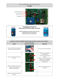
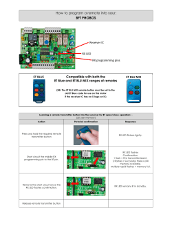


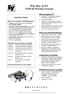

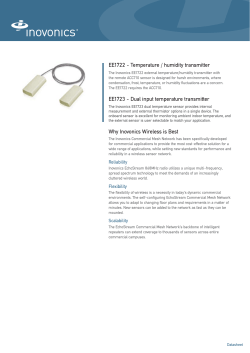


© Copyright 2026