
AB Courseware Sample Telecommunications Radar
Telecommunications
Radar
Courseware Sample
38542-F0
AB
TELECOMMUNICATIONS
RADAR
COURSEWARE SAMPLE
by
the Staff
of
Lab-Volt Ltd.
Copyright © 2007 Lab-Volt Ltd.
All rights reserved. No part of this publication may be reproduced,
in any form or by any means, without the prior written permission
of Lab-Volt Ltd.
Printed in Canada
September 2007
Table of Contents
Introduction . . . . . . . . . . . . . . . . . . . . . . . . . . . . . . . . . . . . . . . . . . . . . . . . . . . V
Courseware Outline
Principles of Radar Systems . . . . . . . . . . . . . . . . . . . . . . . . . . . . . . . . . . . VII
Analog MTI Processing . . . . . . . . . . . . . . . . . . . . . . . . . . . . . . . . . . . . . . . . IX
Digital MTD Processing . . . . . . . . . . . . . . . . . . . . . . . . . . . . . . . . . . . . . . . XII
Tracking Radar . . . . . . . . . . . . . . . . . . . . . . . . . . . . . . . . . . . . . . . . . . . . . . XIV
Radar in an Active Target Environment . . . . . . . . . . . . . . . . . . . . . . . . . . . XVI
The Phased Array Antenna . . . . . . . . . . . . . . . . . . . . . . . . . . . . . . . . . . . . XIX
Sample Exercise Extracted from Principles of Radar Systems
Ex. 2-1
Pulsed Radar Transmitter and Receiver . . . . . . . . . . . . . . . . . . . . 3
The operating principles of a pulsed radar transmitter and receiver.
The Radar Transmitter and Radar Receiver of the Radar Training
System.
Sample Exercise Extracted from Analog MTI Processing
Ex. 2-2
Vector-Processing MTI . . . . . . . . . . . . . . . . . . . . . . . . . . . . . . . . . 25
Blind phases. Elimination of blind phases using vector-processing
MTI.
Sample Exercise Extracted from Digital MTD Processing
Ex. 2-2
Fast Fourier Transform (FFT) Processing . . . . . . . . . . . . . . . . . . 47
Forming digital filters. Velocity sorting. Doppler ambiguities. Blind
(dim) speeds.
Sample Exercise Extracted from Tracking Radar
Ex. 4
Angle Tracking Techniques . . . . . . . . . . . . . . . . . . . . . . . . . . . . . 69
What is angle tracking? Lobe switching technique. Crossover loss.
Conical scan technique. Monopulse technique. Advantages of the
monopulse technique over the lobe switching and conical scan
techniques. Lobe switching implementation in the Lab-Volt Tracking
Radar.
III
Table of Contents (cont'd)
Sample Exercise Extracted from Radar in an Active Target Environment
Ex. 1-5
Antennas in EW: Sidelobe Jamming
and Space Discrimination . . . . . . . . . . . . . . . . . . . . . . . . . . . . . . 93
Presentation of the difference between mainlobe and sidelobe
jamming. Outline of the effects of effective sidelobe noise jamming.
Presentation of certain antenna space discrimination techniques used
as radar EP against stand-off noise jammers.
Sample Exercise Extracted from The Phased Array Antenna
Ex. 1-1
Familiarization with the Phased Array Antenna . . . . . . . . . . . . . 109
Description and use of the Phased Array Antenna (PAA) and the
Phased Array Antenna Controller.
Other Sample Extracted from Principles of Radar Systems
Unit Test . . . . . . . . . . . . . . . . . . . . . . . . . . . . . . . . . . . . . . . . . . . . . . . . . . 119
Instructor Guide Sample Extracted from Radar Training System
Unit 1
Bibliography
IV
Fundamentals of Pulsed Radar . . . . . . . . . . . . . . . . . . . . . . . . . 123
Introduction
The Lab-Volt Radar Training System, Model 8096, is a modular table-top radar
system especially designed for teaching radar in a laboratory classroom. It is a real
radar system, not a simulator, that uses innovative technology to detect passive
targets at very short ranges. The low-power of its transmitter allows safe operation
in a variety of training environments.
The Radar Training System can operate as either one of the following four types of
radars: pulse radar, continuous wave (CW) radar, frequency-modulated continuous
wave (FM-CW) radar, and tracking radar. When operated as a pulse radar, the Ascope and plan position indicator (PPI) displays are available as well as MTI
processing and MTD processing. Only a few connections and settings are required
to rapidly pass from the hands-on study of a pulse radar to that of a CW, FM-CW or
tracking radar.
When used with the Radar Jamming Pod Trainer, the Radar Training System
becomes an efficient tool to train students in the principles and scenarios of
Electronic Warfare (EW). Also, the conventional, mechanically rotated antenna of the
Radar Training System can be replaced with the Phased Array Antenna to provide
students with training in the principles of electronically steered antennas. Finally, the
Radar Training System can be converted into a sophisticated, pulse mode, radar
cross-section (RCS) measurement training system with inverse synthetic aperture
radar (ISAR) capability, by the addition of a few additional components.
The design of the Radar Training System emphasizes functionality, with block
diagrams silk-screened on the module front panels or being displayed on the screen
of the radar host computer. Major inputs and outputs are readily accessible through
various connectors on the front panels. Test points in the instructional modules can
be brought out to the front panel, located on the printed circuit board or made
available in the block diagrams shown on the radar host computer's screen.
Faults can be inserted by the instructor in the instructional modules, for teaching
troubleshooting, through fault switches located on the printed circuit boards of certain
modules or the Faults window which can be displayed on the radar host computer's
screen. The fault switches on the printed circuit boards are accessed through the
hinged door located on top of certain instructional modules. Another hinged panel
inside each of these modules prevents students from accessing the fault switches.
The student courseware for the Radar Training System consists of six volumes. The
courseware covers the following subject matter:
–
The first volume, titled Principles of Radar Systems, deals with the principles and
operation of pulsed, CW, and FM-CW radars.
–
A second volume, titled Analog MTI Processing, covers the principles of analog
signal processing techniques and MTI radar.
–
The next volume in the series, titled Digital MTD Processing, presents modern
digital processing techniques related to those used in air-traffic-control radars.
–
The fourth volume in the series, titled Tracking Radar, explains the principles of
operation of tracking radars (with emphasis on the lobe-switching tracking radar)
and discusses the factors which may affect the range and angle tracking
performance.
–
The fifth volume in the series, titled Radar in an Active Target Environment,
provides instruction in the principles of electronic warfare as applied to search
and tracking radars.
V
Introduction (cont'd)
–
The last volume in the series, titled The Phased Array Antenna, enables the
student to learn about the construction and characteristics of phased array
antennas, and make quantitative measurements of these characteristics.
Furthermore, a user guide is available for those who are using the Radar Training
System as an RCS measurement system with ISAR imagery capability.
An instructor’s guide is also available. This guide provides outlines of the theory
presented in the courseware, and describes many demonstrations that, in most
cases, have not been included in the student manuals. These demonstrations are
a useful complement to radar teaching. The instructor’s guide also provides aids to
the presentation of the various topics covered in the courseware.
The courseware of the Radar Training System has a Unit-Exercise structure. Each
unit of instruction consists of several exercises designed to present material in
convenient instructional segments. Principles and concepts are presented first, and
hands-on procedures complete the learning process to involve and better acquaint
the student with each module, and with complete radar systems.
At the end of each exercise, there is a five-questions review section requiring brief
written answers. Suggested answers for these questions, as well as for those found
in the exercise procedures, are included in the appendices of the student manuals.
Each unit terminates with a ten-question multiple-choice test to verify the knowledge
gained in the unit. The answers for these questions are given in the radar instructor’s
guide only.
VI
Courseware Outline
PRINCIPLES OF RADAR SYSTEMS
Unit 1 Fundamentals of Pulsed Radar
The fundamentals of pulsed radar, including the range-delay relationship,
radar antennas, and the radar equation, as well as safety measures
applicable to all radar systems.
Ex. 1-1 Basic Principles of Pulsed Radar
Basic principles of pulsed radar. Introduction to the Radar Training
System and the A-scope display. Safety measures applicable to all
radar systems.
Ex. 1-2 The Range-Delay Relationship
The relationship between target range and the delay between
pulse transmission and echo reception. The concept of range
resolution. Measuring target range and range resolution using the
A-scope display.
Ex. 1-3 Radar Antennas
The role of the antenna in a radar system. Radar antenna
characteristics. Plotting the radiation pattern and measuring
angular resolution of the radar antenna.
Ex. 1-4 The Radar Equation
The various parameters in the radar equation and their interaction
in a radar system.
Unit 2 A Pulsed Radar System
The transmitter, the receiver, the antenna driving system, and the PPI
display in a pulsed radar system.
Ex. 2-1 Pulsed Radar Transmitter and Receiver
The operating principles of a pulsed radar transmitter and receiver.
The Radar Transmitter and Radar Receiver of the Radar Training
System.
Ex. 2-2 Antenna Driving System
The mechanical aspects and control of a rotating or scanning radar
antenna.
Unit 3 CW Radars
Continuous-wave and frequency-modulated continuous-wave radars.
VII
Courseware Outline
PRINCIPLES OF RADAR SYSTEMS (cont’d)
Ex. 3-1 CW Radar and the Doppler Effect
The principles of CW radar and the Doppler effect. Observation
and quantification of the frequency components associated with
the Doppler effect.
Ex. 3-2 Frequency-Modulated CW Radar
FM ranging using frequency-modulated continuous-wave radar.
The relationship between range and beat frequency.
Unit 4 Troubleshooting Radar Systems
A methodical approach to troubleshooting CW, FM-CW and pulsed radar
systems.
Ex. 4-1 Troubleshooting a CW Radar
A methodical approach to troubleshooting. Troubleshooting
techniques applicable to radar equipment. Locating and diagnosing
instructor-inserted faults in a CW radar.
Ex. 4-2 Troubleshooting an FM-CW Radar
Locating and diagnosing instructor-inserted faults in an FM-CW
radar.
Ex. 4-3 Troubleshooting a Pulsed Radar: The RF Section
Locating and diagnosing instructor-inserted faults in the RF section
of a pulsed radar.
Appendices A
B
C
D
E
F
G
H
I
J
Setting Up the Basic Radar Training System
Calibration of the Radar A-Scope Display
Targets and Radar Cross Section
Operation of the Dual-Channel Sampler
Common Symbols
Module Front Panels
Test Points and Diagrams
Answers to Procedure Step Questions
Answers to Review Questions
Equipment Utilization Chart
Bibliography
We Value Your Opinion!
VIII
Courseware Outline
ANALOG MTI PROCESSING
Unit 1 Analog Radar Systems
The basic concepts of analog pulse radar systems. Familiarization with the
Analog Pulse Radar obtained using the Lab-Volt Radar Training System.
Ex. 1-1 Familiarization with the Analog Pulse Radar
Familiarization with the LVRTS software and with the Analog Pulse
Radar mode of the Radar Processor/Display. Calibration of the
system and use of the software instruments.
Ex. 1-2 The PPI Display
Familiarization with the PPI display and with the various markers
available on the display. Measuring the range resolution and
angular resolution of the radar system.
Unit 2 Analog MTI Radar
The operation and use of analog moving-target indication (MTI) processing
for enhancing the detection of moving targets.
Ex. 2-1 Phase-Processing MTI
The principle of phase detection in a coherent pulsed radar. The
use of phase processing to detect moving targets. The frequency
response of a single delay-line MTI canceller.
Ex. 2-2 Vector-Processing MTI
Blind phases. Elimination of blind phases using vector-processing
MTI.
Ex. 2-3 Staggered PRF
Blind speeds. Second-trace echoes and range ambiguities. The
effect of staggered PRF on blind speeds and second-trace echoes.
The frequency response of a single delay-line canceller in
staggered PRF mode.
Ex. 2-4 MTI Limitations
Factors limiting MTI performance. Parameters used in measuring
MTI performance.
IX
Courseware Outline
ANALOG MTI PROCESSING (cont’d)
Unit 3 Target Detection in Noise and Clutter
The characteristics of noise and clutter and their effects on target detection.
Ex. 3-1 Threshold Detection
Threshold detection of targets. The relationship between
probability of false alarm, probability of detection and
signal-to-noise ratio.
Ex. 3-2 Pulse Integration
The role of pulse integration in radar detection. The operation of
the feedback integrator. Measuring the integration improvement
factor.
Ex. 3-3 Sensitivity Time Control
The role and operation of sensitivity time control in pulsed radar.
Ex. 3-4 Instantaneous Automatic Gain Control
The instantaneous automatic gain control technique used in linear
receivers.
Ex. 3-5 The Log-FTC Receiver
The principle of the log-FTC receiver. The effect of the log-FTC
receiver on target detection in the presence of rain clutter.
Ex. 3-6 Constant False-Alarm Rate
The adaptive threshold technique used to obtain a constant
false-alarm rate.
Unit 4 Troubleshooting
A methodical approach to troubleshooting MTI radar systems.
Ex. 4-1 Troubleshooting the MTI Processor
Troubleshooting techniques. Locating and diagnosing instructorinserted faults in an analog MTI signal processor.
Ex. 4-2 Troubleshooting the Display Processor
Locating and diagnosing instructor-inserted faults in an analog
display processor.
X
Courseware Outline
ANALOG MTI PROCESSING (cont’d)
Ex. 4-3 Troubleshooting an MTI Radar System
Locating and diagnosing instructor-inserted faults in a complete
analog MTI radar system.
Appendices A
B
C
D
E
F
G
H
Setting Up the Radar Training System
Calibration and Adjustment of the Radar Training System
Radar Training System Targets
Common Symbols
Module Front Panels
Test Points and Diagrams
Answers to Procedure Step Questions
Answers to Review Questions
Bibliography
We Value Your Opinion!
XI
Courseware Outline
DIGITAL MTD PROCESSING
Unit 1 Digital Pulse Radar Systems
The fundamentals of digital signal processing. Familiarization with the Digital
Pulse Radar obtained using the Lab-Volt Radar Training System.
Ex. 1-1 Familiarization with the Digital Pulse Radar
The importance of coherence and synchronization of the PRF with
the antenna rotation. Sensitivity time control (STC). Familiarization
with the LVRTS software and with the Digital Pulse Radar mode of
the Radar Processor / Display. Operation in the PPI mode.
Ex. 1-2 The PPI Display
Types of radar displays. The digital PPI display. Generating the
PPI display in the Digital MTD/PPI Processor.
Unit 2 MTD Detection Processing
Techniques involved in first-stage moving-target detection (MTD)
processing.
Ex. 2-1 Cell Mapping
Range-azimuth cells. Coherent processing intervals. Doppler cells.
Clutter maps.
Ex. 2-2 Fast Fourier Transform (FFT) Processing
Forming digital filters. Velocity sorting. Doppler ambiguities. Blind
(dim) speeds.
Ex. 2-3 Constant False-Alarm Rate (CFAR)
Adaptive thresholding. Time-average and cell-average CFAR.
Target detection in a noisy environment.
Unit 3 Alarm Processing
Techniques involved in second- and third-stage MTD processing.
Ex. 3-1 Correlation and Interpolation (C&I) Processing
Clustering and correlation of primitive target reports. Centroiding.
Interpolation.
Ex. 3-2 Surveillance (Track-While-Scan) Processing
Processing steps used in surveillance processing. Track scoring.
XII
Courseware Outline
DIGITAL MTD PROCESSING (cont’d)
Unit 4 Troubleshooting
A methodical approach to troubleshooting digital radar systems.
Ex. 4-1 Troubleshooting the Digital MTD/PPI Processor
Locating and diagnosing instructor-inserted faults in the Digital
MTD/PPI Processor.
Appendices
A
B
C
Setting Up the Radar Training System
Calibrating the Radar Training System
Answers to Procedure Step Questions
Bibliography
We Value Your Opinion!
XIII
Courseware Outline
TRACKING RADAR
Exercise 1
Familiarization with the Tracking Radar
What is a tracking radar? Track-while-scan (TWS) radar versus
continuous tracking radar. Basic operation of a tracking radar. The
Lab-Volt Tracking Radar Training System. The Lab-Volt Radar
Training System (LVRTS) software. Operating the Lab-Volt Tracking
Radar.
Exercise 2
Manual Tracking of a Target
Manual tracking of a target. Range gate, range gate marker, and
O-scope display. Manual control of the antenna and range gate
positions in the Lab-Volt Tracking Radar.
Exercise 3
Automatic Range Tracking
Principle of automatic range tracking. Applications of range trackers.
Target search and acquisition. Split range-gate tracking. Leadingedge range tracking and trailing-edge range tracking. Range tracking
rate limitation. Operation of the range tracker in the Lab-Volt Tracking
Radar.
Exercise 4
Angle Tracking Techniques
What is angle tracking? Lobe switching technique. Crossover loss.
Conical scan technique. Monopulse technique. Advantages of the
monopulse technique over the lobe switching and conical scan
techniques. Lobe switching implementation in the Lab-Volt Tracking
Radar.
Exercise 5
Automatic Angle Tracking
Principle of automatic angle tracking. Operation of the angle tracker
in the Lab-Volt Tracking Radar. Angular error voltage versus the
angular error in the Lab-Volt Tracking Radar.
Exercise 6
Range and Angle Tracking Performance
(Radar-Dependent Errors)
Resolution, precision, and accuracy of tracking radars. Radardependent errors. Effect of the receiver thermal noise and antenna
servosystem noise and limitations on the tracking error. Use of an
AGC circuit to reduce the variation of the echo amplitude due to target
range and fluctuations of the target radar cross section.
XIV
Courseware Outline
DIGITAL MTD PROCESSING (cont’d)
Exercise 7
Range and Angle Tracking Performance
(Target-Caused Errors)
Amplitude scintillation. Effect of the amplitude scintillation on the
angular tracking error in lobe switching and conical scan tracking
radars. Angular scintillation (glint). Effect of the angular scintillation on
the angular tracking error. Principle of frequency agility. Use of
frequency agility to reduce the angular tracking error.
Exercise 8
Troubleshooting a Radar Target Tracker
Use of a methodical approach to locate and diagnose instructorinserted faults in the Radar Target Tracker of the Lab-Volt Tracking
Radar.
Appendices A Setting Up the Tracking Radar Training System
B Calibration and Adjustment of the Tracking Radar Training
System
C Answers to Procedure Step Questions
D Answers to Review Questions
Bibliography
We Value Your Opinion!
XV
Courseware Outline
RADAR IN AN ACTIVE TARGET ENVIRONMENT
Unit 1
Noise Jamming
The context of electronic warfare in modern conflicts. Introduction to
electronic warfare and its subdivisions (EA, EP, ES). The relationship
between the subdivisions.
Ex. 1-1 Familiarization with the Radar Jamming Pod Trainer
Familiarization with the various controls, input/output connectors,
and accessories on the Radar Jamming Pod Trainer. Radar
Jamming Pod Trainer properties and jamming signal capabilities.
Ex. 1-2 Spot Noise Jamming and Burn-Through Range
Description of spot noise jamming. Difference between the selfscreening, mutual-support, escort, and stand-off EA missions.
The concept of burn-through range. Introduction of the radar
range equation modified for spot noise jamming.
Ex. 1-3 Frequency Agility and Barrage Noise Jamming
Discussion relating to the radar receiver passband. Introduction
to frequency agility as an electronic protection against spot noise
jamming. Description of barrage noise jamming. Justification of
the use of barrage noise jamming against frequency-agile radars.
Ex. 1-4 Video Integration and Track-On-Jamming
The importance of signal discrimination (signal processing
techniques) used as radar EPs against noise jamming. A case
example, the effects of video integration when used by a radar
confronted with noise jamming. Discussion of the jammer strobe.
The angle track-on jamming capability of certain radars.
Ex. 1-5 Antennas in EW: Sidelobe Jamming
and Space Discrimination
Presentation of the difference between mainlobe and sidelobe
jamming. Outline of the effects of effective sidelobe noise
jamming. Presentation of certain antenna space discrimination
techniques used as radar EP against stand-off noise jammers.
Unit 2
Range Deception Jamming
The fundamental differences between noise jamming and deception
jamming. Presentation of the different categories of deceptive jamming.
Comparison between range deception and angle deception jamming
techniques.
XVI
Courseware Outline
RADAR IN AN ACTIVE TARGET ENVIRONMENT (cont’d)
Ex. 2-1 Deception Jamming Using the Radar Jamming Pod
Trainer
Generating false targets with the Radar Jamming Pod Trainer.
Familiarization with the RGPO and the on-off modulation
capabilities of the Jamming Pod.
Ex. 2-2 Range Gate Pull-Off
The implementation of range DECM against radars that use split
range-gate tracking. Introduction to range gate pull-off (RGPO),
and the phases of an RGPO jamming cycle. Use of a range-rate
tracking limiter as an EP against unrealistic RGPO. Use of
leading-edge range tracking as an EP against RGPO.
Ex. 2-3 Stealth Technology: The Quest for Reduced RCS
Introduction to the basic material and design principles behind
radar stealth technology. The role of hard-body shaping and radar
absorbent materials (RAM) in the implementation of these
principles. Implications of stealth technology to electronic warfare.
Unit 3
Angle Deception Jamming
Reasons that angle and range DECM are implemented together against
tracking radars. Differentiation between those angle deception techniques
used against conical scanning and sequential lobing radars, and those
used against monopulse radars. Introduction to silent lobing as an EP.
Ex. 3-1 Deceptive Jamming Using
Amplitude-Modulated Signals
The principles of inverse gain jamming as used against conical
scan and sequential lobing angular tracking systems. Distinction
between asynchronous/synchronous inverse gain jamming and
AM noise. The importance of lobing/scanning rate agility as a
radar EP against amplitude-modulation angle deception
techniques.
Ex. 3-2 Cross-Polarization Jamming
The main reason for the existence of the cross-polarized (Condon
lobes) antenna radiation pattern. Comparison between typical
parabolic antenna cross- and co-polarized antenna patterns.
Introduction to cross-polarization jamming.
XVII
Courseware Outline
RADAR IN AN ACTIVE TARGET ENVIRONMENT (cont’d)
Ex. 3-3 Multiple-Source Jamming Techniques
The mutual support EA mission and its relation to cooperative
jamming techniques. How multiple-source jamming techniques
induce artificial glint onto the jamming signal. Distinction between
coherent and incoherent multiple-source jamming. The difference
between formation and blinking jamming, and how victim radars
use angle-rate limiters as electronic protection.
Unit 4
Chaff
Fundamentals of chaff physics, and reasons why the Lab-Volt variabledensity chaff cloud (VDCC) reproduces the effects of chaff. Dispensing and
uses of chaff. Chaff placed within its historical context.
Ex. 4-1 Chaff Clouds
Corridor dispensing of chaff. Discrimination of chaff echoes using
radar MTI processing. Setting-up the Lab-Volt Variable-Density
Chaff Cloud (VDCC).
Ex. 4-2 Chaff Clouds used as Decoys
Burst dispensing of chaff to create false targets. Introduction to
jammer-illuminated chaff (JAFF). Defeating the processing ability
of MTI radars via the noisy Doppler frequency imparted to chaff
clouds via JAFF.
Appendices
A Setting Up the Tracking Radar Training System
B Calibration and Adjustment of the Tracking Radar Training
System
C Answers to Procedure Step Questions
D Answers to Review Questions
E Glossary
F EWT Accessories
Bibliography
We Value Your Opinion!
XVIII
Courseware Outline
THE PHASED ARRAY ANTENNA
Unit 1
Basic Operation
Ex. 1-1 Familiarization with the Phased Array Antenna
Description and use of the Phased Array Antenna (PAA) and the
Phased Array Antenna Controller.
Ex. 1-2 The True Time-Delay Rotman Lens
Principles of the Rotman lens.
Ex. 1-3 The Switching Matrix
Operation of the RF switching matrix.
Unit 2
Measurement of Phased Array Antenna
Characteristics
Ex. 2-1 Beamwidth Measurement
Measuring the 3-dB beamwidth of the PAA.
Ex. 2-2 Radiation Pattern Measurement
Measuring and plotting the PAA radiation pattern.
Ex. 2-3 Angular Separation Measurement
Measuring the angular separation between two consecutive PAA
beams.
Ex. 2-4 Phased Array Antenna Gain Measurement
Measuring the PAA gain for various beams (center and end). PAA
gain versus scan angle.
Ex. 2-5 Maximum Scan Angle Measurement
Measuring the maximum scan angle of the PAA.
Ex. 2-6 Target Bearing Estimation
Estimating the target position relative to a selected beam.
Ex. 2-7 Target Speed Estimation
Calculating the speed of a target moving perpendicularly to the
radar line of sight, using the angular displacement and the PAA
scan speed.
XIX
Courseware Outline
THE PHASED ARRAY ANTENNA (cont’d)
Appendices
A Setting Up the Radar Training System with the PAA
B Calibration and Adjustment of the Radar Training System
with the PAA
C Answers to Procedure Step Questions
D Answers to Review Questions
E Glossary
F Equipment Utilization Chart
Bibliography
We Value Your Opinion!
XX
Sample Exercise
Extracted from
Principles of Radar Systems
Exercise
2-1
Pulsed Radar Transmitter and Receiver
EXERCISE OBJECTIVE
When you have completed this exercise, you will be familiar with the operating
principles of a pulsed radar transmitter and receiver. You will also be familiar with the
Radar Transmitter and Radar Receiver of the Lab-Volt Radar Training System.
DISCUSSION
Radar Transmitters
The purpose of the transmitter in a pulsed radar system is to produce a pulsed RF
signal which can be transmitted by the antenna. The RF signal is generated either
by a high-power RF oscillator, or a low-power RF oscillator followed by an RF
amplifier.
The high-power oscillator converts pulses of dc power directly to pulsed RF at
microwave frequencies, as shown in Figure 2-2 (a). The most commonly used
high-power RF oscillator in radar is the magnetron. This is a type of vacuum tube
oscillator developed near the beginning of World War II. It is widely used because
of its simplicity, ruggedness and efficiency. Its name comes from the fact that it uses
a magnetic field to modify the trajectory of electrons in motion.
Figure 2-2 (b) shows a low-power RF master oscillator followed by a power amplifier.
The amplifier accepts the low-power RF signal and amplifies it to produce a
high-power signal. One common type of high-power amplifier used in radar
transmitters is the gridded traveling wave tube amplifier. A control grid inside this
tube acts as a modulator and allows a low-power pulse signal to key the amplifier on
and off.
A simplified block diagram of the Lab-Volt Radar Transmitter is shown in
Figure 2-2 (c). A solid-state RF oscillator produces a low-power RF signal. This
signal is not amplified, but is simply modulated by a modulator to produce low-power
radar pulses.
3
Pulsed Radar Transmitter and Receiver
Figure 2-2. Generation of radar pulses.
Figure 2-3 shows the waveforms present in a pulsed radar transmitter, where a pulse
train is used to modulate a continuous, sinusoidal RF carrier. Typical carrier
frequencies for conventional radars range from 220 MHz to 35 GHz. The modulating
pulses are rectangular, although somewhat rounded due to bandwidth limitations.
The resulting waveform is a pulsed sine wave.
4
Pulsed Radar Transmitter and Receiver
Figure 2-3. Signal waveforms in a pulsed radar transmitter.
The pulse repetition frequency (PRF, or fp) is the number of pulses transmitted per
unit time. Typical PRF's range from several hundred hertz to several hundred
kilohertz. The interpulse period T is equal to 1/fp.
The pulse width τ is the pulse duration. It is usually defined as the time interval
between the points where the instantaneous value equals 50% of the peak
amplitude. Typical pulse widths range from 0.02 µs to 60 µs, with 1 µs being a
common value.
The peak power of a pulsed radar signal is equal to the power of the individual
pulses (i.e. power when the transmitter is transmitting). The average power is
where Pavg
Ppeak
τ
T
is the average power
is the peak power
is the pulse width
is the interpulse period.
The average power can be thought of as the energy per pulse Ppeak x τ divided by the
interpulse period T, or as the peak power multiplied by the duty factor of the
transmitter τ/T.
5
Pulsed Radar Transmitter and Receiver
The maximum detection range of a radar is partly determined by the total amount of
energy transmitted per unit time, i.e. the average power. To increase detection
range, average power can be increased by increasing either the peak power or the
pulse width, thus increasing the energy per pulse. As was seen in Exercise 1-2,
however, increasing the pulse width deteriorates the range resolution of the radar.
Increasing the PRF, without changing the pulse width, also increases the average
power, but for reasons which will be explained in a later volume, decreases the
maximum range at which the target range can be accurately determined.
Radar receivers
Most radar receivers operate by detecting the envelope of the received signal in
order to recover the original modulating waveform. Envelope detection is illustrated
in Figure 2-4. The high frequency carrier is removed from the signal, and only the
positive portion of the envelope is retained. The detected pulses are then amplified
for further processing and display.
Figure 2-4. Envelope detection.
Envelope-detecting receivers can be divided into two main types: tuned radio
frequency (TRF) and superheterodyne. In a TRF receiver, the envelope detection is
carried out directly at the RF frequency, as shown in Figure 2-5. This type of receiver
is seldom used, since it is generally more costly than a superheterodyne receiver
with equal performance.
Figure 2-5. Tuned radio frequency (TRF) receiver.
The most commonly used type of radar receiver is the superheterodyne receiver,
shown in Figure 2-6. In this type of receiver, the received signal is mixed with a local
oscillator signal. The mixer produces a signal at a frequency equal to the difference
between the RF signal frequency and the local oscillator frequency. This
intermediate frequency (IF) is much lower than the original RF signal frequency. The
IF signal is amplified and filtered by an IF amplifier before the envelope detection
takes place.
6
Pulsed Radar Transmitter and Receiver
Figure 2-6. Superheterodyne receiver.
Because the envelope detection takes place at a relatively low intermediate
frequency, the superheterodyne receiver is less costly and more flexible than a TRF
receiver. Many variations of the basic superheterodyne design are used in radar
systems. Often, the RF signal is applied directly to the mixer without amplification,
in order to reduce the cost of the receiver. This, however, reduces the sensitivity of
the receiver.
In certain radar applications, envelope detection alone does not satisfy the system
requirements. In this case, a quadrature detector is often used. This type of detector
is capable of detecting the phase of the received signal as well as the amplitude.
Figure 2-7 shows a typical quadrature detector. The input signal is either the RF
signal directly from the antenna, or an IF signal. The input signal is divided between
two channels, each having a mixer. In both channels, the input signal is mixed with
a reference signal from the local oscillator. However, a phase shift is introduced so
that the two reference signals are in quadrature (90E out of phase).
Figure 2-7. Quadrature detector.
As the range of a target varies, the amplitude of the detected pulse varies between
a positive and negative maximum. This was observed in Unit 1 using the A-scope
display. With a quadrature detector, the two output signals are in quadrature. When
a pulse in the I (in-phase) channel is at a maximum amplitude, the same pulse in the
Q (quadrature) channel is at a null (zero amplitude). If the target range changes
slightly so that the pulse in the I channel is at a null, the pulse in the Q channel will
be at a maximum, either positive or negative depending on the design of the receiver
and the direction of target motion.
7
Pulsed Radar Transmitter and Receiver
The I and Q pulses from a quadrature detector are never at a null at the same time.
In many receivers, the I and Q signals are eventually combined to produce a unipolar
pulse signal whose amplitude is independent of the phase of the echo signal.
Together, the I and the Q output signals fully represent the phase and amplitude
information contained in the received signal. Radar systems using digital signal
processing techniques often require both amplitude and phase information. For this
reason, quadrature detection is becoming more and more common in modern radar
systems. A receiver which detects both the amplitude and phase of the received
signal is said to be a coherent receiver.
A superheterodyne receiver translates the received signal to an intermediate
frequency. In some receivers, however, the received signal is translated directly to
the baseband (dc) without passing through an intermediate frequency. This is
accomplished by applying the received RF signal to the mixer(s), and using a local
oscillator signal at the same frequency as the RF signal. The mixer produces a signal
at a frequency equal to the difference frequency, which is zero (dc), thus recovering
the modulating waveform in one step. This type of receiver is known as a
homodyne, or DC-IF receiver.
The Lab-Volt Radar Transmitter
The front panel of the Radar Transmitter is shown in Figure 2-8. The carrier
frequency is determined by the FREQUENCY controls in the RF OSCILLATOR
section. When set to VAR., the frequency can be adjusted manually from 8 to
10 GHz. In the CAL. position, the carrier frequency is set to a calibrated 9.4 GHz. In
the MOD. position, the carrier frequency is modulated according to the FREQUENCY
MODULATION controls. Frequency modulation, however, is not used during pulsed
operation. At all times, the voltage at the CONTROL VOLTAGE MONITOR OUTPUT
is a linear function of the carrier frequency.
The ISOLATOR passes RF power in one direction only. It is used to protect the RF
OSCILLATOR from RF power that could be reflected in a backwards direction.
The RF POWER switch allows the RF power to be switched on or off. When in the
STANDBY position, no RF power reaches the DIRECTIONAL COUPLER, and the
STANDBY LED is lit. When in the ON position, the RF power is passed and the ON
LED flashes on and off.
8
Pulsed Radar Transmitter and Receiver
Figure 2-8. The Radar Transmitter.
The DIRECTIONAL COUPLER divides the RF power and sends part of it to the RF
OSCILLATOR OUTPUT. This output provides the local oscillator signal for the Radar
Receiver. The rest of the RF power is available at the CW / FM-CW RF OUTPUT.
The RF power at this output is continuous.
If pulsed operation is desired, the continuous RF power is coupled to the CW RF
INPUT of the MODULATOR. The MODULATOR uses pulses received from the
PULSE GENERATOR to modulate the RF waveform. The resulting pulsed RF signal
is available at the PULSED RF OUTPUT.
The PULSE GENERATOR generates very short pulses which are synchronized with
the pulses at the TRIGGER INPUT. The PULSE WIDTH can be set to 1, 2, or 5 ns,
or to VARiable. The TRIGGER INPUT signal is a synchronization signal supplied by
the Radar Synchronizer.
The Lab-Volt Radar Receiver
The front panel of the Radar Receiver is shown in Figure 2-9. This receiver contains
a quadrature detector. Since the quadrature detector of the Radar Receiver
produces I and Q signals which represent both the amplitude and phase of the
received signal, this receiver can be considered to be coherent.
The POWER DIVIDER at the RF INPUT divides the received RF signal, which is
then sent to two mixers. The HYBRID JUNCTION divides the LOCAL OSCILLATOR
signal into two reference signals which are in quadrature. These reference signals
are sent to their respective mixers.
The LOCAL OSCILLATOR signal comes from the RF OSCILLATOR OUTPUT of
the Radar Transmitter. (See Figure 2-8.) This signal is derived directly from the RF
signal produced by the RF OSCILLATOR. Since the LOCAL OSCILLATOR signal
is at the same frequency as the transmitted and received RF signals, the mixers
9
Pulsed Radar Transmitter and Receiver
translate the received RF signal directly to the baseband. Therefore, this receiver is
of the homodyne type.
Figure 2-9. The Radar Receiver.
The two POWER DIVIDERS following the mixers divide the mixer output signals to
provide the signals required for the various outputs. The PULSED OUTPUT signals
are amplified by the two WIDEBAND AMPLIFIERs. The 1-kHz FILTERS, and the
CW DOPPLER and FM-CW OUTPUTs are not used in pulsed operation.
Procedure Summary
In the first part of this exercise, you will determine the relationship between the
control voltage and frequency of the Radar Transmitter RF OSCILLATOR by
measuring the control voltage for various frequencies, and then plotting the relation
on a graph. You will also observe the shape of the Radar Transmitter PULSE
GENERATOR output signal for various pulse widths, using the Dual-Channel
Sampler, and calculate the duty factor of this signal according to the settings made
on the Radar Training System. The block diagram of the system used to sample the
PULSE GENERATOR output signal is shown in Figure 2-12.
In the second part of this exercise, you will set up a basic pulsed radar and calibrate
the A-scope display. The block diagram of this system is shown in Figure 2-14.
In the third part of this exercise, you will observe a target blip on the A-scope display
while varying the pulse width on the Radar Transmitter, in order to compare the
shape of the target blip with that of the PULSE GENERATOR output signal. You will
also observe the I- and Q-CHANNEL PULSED OUTPUT signals of the Radar
Receiver simultaneously to determine the phase relationship between these two
signals. You will finally observe the role of the reference (local oscillator) signal in the
frequency translation of the received RF signal to baseband, by disconnecting the
LOCAL OSCILLATOR INPUT signal.
10
Pulsed Radar Transmitter and Receiver
Note: In this exercise, you are often asked to set the target range so that the
amplitude of the target blip observed on the A-scope display is positive and
maximum. However, with time, the amplitude of the target blip may vary. This
is due to the RF OSCILLATOR of the Radar Transmitter which may experience
a slight frequency drift with temperature.
To reduce drift to a minimum, it is preferable to let the Radar Training System
warm up for at least half an hour before beginning this exercise. If the amplitude
of the target blip still varies significantly, slightly readjust the target range as
required.
PROCEDURE
The Radar Transmitter
G
1. The main elements of the Radar Training System, that is the antenna and
its pedestal, the target table and the training modules, must be set up
properly before beginning this exercise. Refer to Appendix A of this manual
for setting up the Radar Training System, if this is not done yet.
Set up the modules on the Power Supply / Antenna Motor Driver as shown
in Figure 2-10.
Figure 2-10. Module Arrangement.
On the Radar Transmitter, make sure that the RF POWER switch is in the
STANDBY position.
On the Antenna Controller, make sure that the MANual ANTENNA
ROTATION MODE push button is depressed and that the SPEED control
is in the 0 position.
Set the POWER switch of the Power Supply to the I (on) position, and then
those of the other modules.
11
Pulsed Radar Transmitter and Receiver
G
2. Connect the CONTROL VOLTAGE MONITOR OUTPUT of the Radar
Transmitter to channel 1 of the oscilloscope. This output provides a signal
which is identical with that controlling the RF OSCILLATOR frequency.
On the Radar Transmitter, depress the VARiable FREQUENCY push
button, then set the RF OSCILLATOR frequency to minimum.
Make the appropriate settings on the oscilloscope to observe the CONTROL
VOLTAGE MONITOR OUTPUT signal.
G
3. On the Radar Transmitter, set the RF OSCILLATOR frequency to 8.2 GHz.
Measure the dc voltage at the CONTROL VOLTAGE MONITOR OUTPUT
of the Radar Transmitter, then note the result in the first row of the
CONTROL VOLTAGE column of Table 2-1.
Carry out the same manipulations for the other frequencies listed in
Table 2-1.
CONTROL
VOLTAGE
FREQUENCY
V dc
GHz
8.2
8.6
9
9.4
9.8
Table 2-1. Control voltage versus frequency for the RF OSCILLATOR of the Radar Transmitter.
G
4. In Figure 2-11, plot the relation between the frequency and control voltage
of the RF OSCILLATOR, using the results noted in Table 2-1.
Describe the relationship between the control voltage and frequency of the
RF OSCILLATOR. Determine the slope of this relationship.
12
Pulsed Radar Transmitter and Receiver
Figure 2-11. Relation between the control voltage and frequency for the RF OSCILLATOR of the
Radar Transmitter.
G
5. Remove the cable connecting the CONTROL VOLTAGE MONITOR
OUTPUT of the Radar Transmitter to the oscilloscope.
Figure 2-12 shows how to connect the Dual-Channel Sampler in order to
sample the output signal of the Radar Transmitter PULSE GENERATOR.
Connect the modules as shown in this figure.
Note: Use a medium-length (approximately 75 cm) SMA cable to
connect the PULSE GENERATOR OUTPUT of the Radar
Transmitter to the I-CHANNEL PULSE INPUT of the DualChannel Sampler.
13
Pulsed Radar Transmitter and Receiver
Figure 2-12. Block diagram of the system used for sampling the output signal of the Radar
Transmitter PULSE GENERATOR.
G
6. Make the following adjustments:
On the Radar Transmitter
RF OSCILLATOR FREQUENCY . . . . . . . CAL.
PULSE GENERATOR PULSE WIDTH . . 1 ns
On the Radar Synchronizer
PRF MODE . . . . . . . . . . . . . . . . . . . . SINGLE
PRF . . . . . . . . . . . . . . . . . . . . . . . . . . . 216 Hz
On the oscilloscope
Time Base . . . . . . . . . . . . . . . . . . . . . . . . . X-Y
Channel X . . . . . . . . . . 0.2 V/DIV (DC coupled)
Channel Y . . . . . . . . . . 0.2 V/DIV (Set to GND)
Set the X- and Y-position controls of the oscilloscope so that the trace is
centred on the screen.
Set the Y-channel input coupling switch of the oscilloscope to the
DC position. If an offset voltage is present at the I-CHANNEL SAMPLED
OUTPUT of the Dual-Channel Sampler, the trace on the oscilloscope screen
will shift up or down. If this happens, adjust the I-CHANNEL DC OFFSET
control of the Dual-Channel Sampler so that the trace is centred on the
oscilloscope screen.
14
Pulsed Radar Transmitter and Receiver
Figure 2-13. Output signal of the PULSE GENERATOR for various PULSE WIDTH settings, sampled
with the Dual-Channel Sampler.
15
Pulsed Radar Transmitter and Receiver
G
7. On the Dual-Channel Sampler, select the 1.8-m RANGE SPAN, make sure
that the GAIN controls are in the CALibrated position, then set the ORIGIN
control so that the output signal of the PULSE GENERATOR is centred on
the fourth division of the oscilloscope screen.
On the Radar Transmitter, vary the PULSE WIDTH setting of the PULSE
GENERATOR while observing its output signal on the oscilloscope screen,
then set the PULSE WIDTH to 1 ns. Figure 2-13 shows an example of what
you might observe on the oscilloscope screen for various PULSE WIDTH
settings.
Using the PULSE WIDTH and the actual PRF, calculate the actual duty
factor of the pulse signal provided by the PULSE GENERATOR. Recall that
the actual PRF is 1024 times the PRF selected on the Radar Synchronizer,
as explained in Appendix D.
Setting up the basic pulsed radar
G
8. Remove the SMA cable and the 50 Ω load from the PULSE INPUTS of the
Dual-Channel Sampler.
Figure 2-14 shows the block diagram of the basic pulsed radar that can be
obtained using the Radar Training System. Connect the modules according
to this block diagram.
G
9. Refer to Appendix B of this manual to calibrate the A-scope display so that
its origin is located approximately 1.0 m from the antenna horn and its range
span is equal to 1.8 m. Once you have finished the calibration, the display
on the oscilloscope should resemble Figure 2-15.
The Radar Receiver
G 10. On the Target Controller, use the Y-axis POSITION control to place the
target at the far end of the target table, then vary the target range by a few
millimeters so that the peak voltage of the target blip on the A-scope display
is positive and maximum.
16
Pulsed Radar Transmitter and Receiver
Figure 2-14. Block diagram of the basic pulsed radar.
17
Pulsed Radar Transmitter and Receiver
Figure 2-15. Calibrated A-scope display of a fixed target located at the origin.
On the Radar Transmitter, vary the PULSE WIDTH setting of the PULSE
GENERATOR while observing the target blip on the A-scope display, then
set the PULSE WIDTH to 1 ns. Figure 2-16 shows an example of what you
might observe on the oscilloscope screen for various PULSE WIDTH
settings.
Compare the shape of the target blip with that of the PULSE GENERATOR
output signal. Are they alike? Why?
G 11. On the oscilloscope, disconnect the end of the cable connected to
channel X, then connect it to the external triggering input.
Connect the I- and Q-CHANNEL SAMPLED OUTPUTS of the Dual-Channel
Sampler to channels 1 and 2 of the oscilloscope, respectively.
Make the appropriate settings on the oscilloscope to obtain a stable display
of the I- and Q-CHANNEL PULSED OUTPUT signals of the Radar
Receiver. These signals are presently sampled by the Dual-Channel
Sampler.
18
Pulsed Radar Transmitter and Receiver
Figure 2-16. Fixed target blip for various PULSE WIDTH settings on the Radar Transmitter.
19
Pulsed Radar Transmitter and Receiver
Figure 2-17 shows an example of what you might observe on the
oscilloscope screen.
Figure 2-17. I- and Q-CHANNEL PULSED OUTPUT signals of the Radar Receiver.
On the Target Controller, use the Y-axis POSITION control to slowly
decrease the target range so that the amplitude of the I-CHANNEL PULSED
OUTPUT signal passes from a positive maximum to a negative maximum
and then to another positive maximum. While doing this, observe both
signals on the oscilloscope screen.
Describe what you observe on the oscilloscope screen.
Describe the relationship between the I- and Q-CHANNEL PULSED
OUTPUT signals.
20
Pulsed Radar Transmitter and Receiver
What is the cause of the phase relationship between the I- and
Q-CHANNEL PULSED OUTPUT signals?
G 12. On the Radar Transmitter, place the RF POWER switch in the STANDBY
position.
On the Radar Receiver, disconnect the end of the SMA cable connected to
the LOCAL OSCILLATOR INPUT.
On the Radar Transmitter, place the RF POWER switch in the ON position.
Observe the oscilloscope screen. Are there any signals at the I- and
Q-CHANNEL PULSED OUTPUT? Why?
G 13. On the Radar Transmitter, make sure that the RF POWER switch is in the
STANDBY position. The RF POWER STANDBY LED should be lit. Place
all POWER switches in the O (off) position and disconnect all cables.
CONCLUSION
In this exercise, you plotted the relationship between the control voltage and
frequency of the RF OSCILLATOR. You found that the frequency of the RF OSCILLATOR varies linearly at a rate of 0.25 GHz per volt as the control voltage varies.
You observed that the shape of the target blip resembles that of the PULSE
GENERATOR output signal, since the Radar Receiver detects the envelope of the
received signal.
You also observed the I- and Q-CHANNEL PULSED OUTPUT signals of the Radar
Receiver simultaneously and found that these signals are in quadrature. Finally, you
verified that a reference (local oscillator) signal is required to carry out the frequency
translation of the received RF signal to baseband.
21
Pulsed Radar Transmitter and Receiver
REVIEW QUESTIONS
1. Why is the magnetron the most commonly used high-power RF oscillator in
radar?
2. Describe the usual waveform of the transmitted radar signal.
3. How do most radar receivers operate?
4. What is the main advantage of a superheterodyne receiver over a tuned radio
frequency (TRF) receiver?
5. What is the main advantage of the quadrature detector?
22
Sample Exercise
Extracted from
Analog MTI Processing
Exercise
2-2
Vector-Processing MTI
EXERCISE OBJECTIVE
When you have completed this exercise, you will be familiar with phenomenon of
blind phases and their elimination using vector-processing MTI.
DISCUSSION
Blind Phases
A phase-processing MTI system consists of a coherent radar with one delay-line
canceller, as shown in Figure 2-27. In this system, the received RF echo signal is
heterodyned in the phase detector with the coherent reference signal. The amplitude
of each pulse in the coherent video signal (the phase detector output signal) is a
function of the phase and amplitude of the echo signal. If the target is moving, the
changing phase of the echo signal causes the amplitude of the coherent video signal
to vary from pulse to pulse.
The coherent video is processed using a delay-line canceller which suppresses the
pulses corresponding to fixed targets. The cancelled video, which contains only
moving-target information, is full-wave rectified before display on a PPI.
Figure 2-27. Phase-processing MTI radar with homodyne receiver.
With a moving target, the coherent video at the output of the phase detector consists
of pulses with a sine-wave envelope, as shown in Figure 2-28 (a). If the phases of
the echoes are such that two successive pulses in the video signal have the same
25
Vector-Processing MTI
amplitude, these pulses are cancelled by the delay-line canceller, even though the
target is moving. This results in a pulse of zero amplitude in the cancelled video, as
shown in (b). This phenomenon is known as blind phases.
Figure 2-28. The blind-phases phenomenon.
Blind phases can cause nulls in the unipolar video signal, as seen in
Figure 2-28 (c). This results in reduced sensitivity of the radar. Even if the phases
are such that no pulses are completely cancelled, the fact that the amplitude of the
26
Vector-Processing MTI
unipolar video signal drops periodically causes a loss of sensitivity. The problem of
reduced sensitivity caused by blind phases can be eliminated by using a quadrature
phase detector.
Quadrature phase detector
The envelope of the received signal in a pulsed radar is
vrec= A sin [2π(ft ± fd)t + n0]
= A sin (2πftt + n)
where
vrec
A
ft
fd
n0
n
(1)
is the received signal waveform,
is the amplitude of the received signal,
is the transmitted frequency,
is the Doppler frequency,
is the phase shift due to the target range,
is the phase of the received signal relative to the reference signal.
As shown in Figure 2-29, the received signal A sin (2πftt + n) can be represented as
a vector of length A and angle n. This vector can be broken down into two
components in phase quadrature: the in-phase component I = A cos n and the
quadrature component Q = A sin n.
Figure 2-29. Phasor diagram of the received signal.
The quadrature phase detector, or I and Q detector, detects both the in-phase and
the quadrature components of the received signal separately. As seen in
Figure 2-30, this type of detector has two channels: the I (in-phase) channel and the
Q (quadrature) channel.
The I channel is identical to the single-channel phase detector in Figure 2-27. In
channel Q, however, the coherent reference signal undergoes a phase shift of 90E
27
Vector-Processing MTI
before being applied to the phase detector. The coherent reference signals are
therefore in phase quadrature:
I-channel coherent reference = k sin 2πftt
(2)
Q-channel coherent reference = k cos 2πftt
(3)
where
k is the amplitude of the reference signals,
ft is the frequency of the reference signal (in a homodyne receiver; in a
superheterodyne receiver, the reference signal would be at t h e
intermediate frequency.)
Figure 2-30. Quadrature phase detector.
The I-channel output of the quadrature detector is the in-phase component of the
signal A cos n. In the Q channel, heterodyning the received signal A sin (2πftt + n)
and the phase-shifted reference signal k cos 2πftt yields the quadrature component
A sin n. Together, the in-phase and quadrature components define the vector which
represents the received signal. Each component of this vector is processed in a
separate delay-line canceller for MTI. This is called vector-processing MTI.
28
Vector-Processing MTI
Figure 2-31. Vector-processing MTI receiver.
29
Vector-Processing MTI
Vector-processing MTI
Figure 2-31 shows the receiver section of a homodyne vector-processing MTI radar.
There is a delay-line canceller for each of the I and Q channels. The outputs of the
I- and Q-channel cancellers are combined in the magnitude detector to produce a
unipolar video signal.
The operation of the vector-processing MTI receiver can be explained as follows. If
a target at range R0 is moving, the phase n of the signal at the input of the
quadrature detector input is a function of time and of the Doppler frequency:
n (moving target) = ±2πfdt + n0
where
(4)
fd is the Doppler frequency,
n0 is the phase shift due to the range R0.
Assuming the Doppler frequency is positive, the envelopes of the pulse trains at the
I and Q outputs of the quadrature detector are therefore
I
= A cos n
= A cos (2πfdt + n0)
(5)
Q = A sin n
= A sin (2πfdt + n0)
where
(6)
I and Q are the envelopes of the I- and Q-channel output signals of the
quadrature detector,
A is the amplitude of the received echo signal,
fd is the Doppler frequency of the received echo signal,
n0 is the phase shift due to the range R0.
These two waveforms are illustrated in Figure 2-32 (a) and (b) respectively. They are
identical except for a 90E phase shift. The Doppler period 1/fd and the
pulse-repetition interval T = 1/fp are shown in the figure.
In the delay-line cancellers, each pulse is stored for one pulse repetition interval and
then subtracted from the following pulse. Consider two successive pulses at the input
of the I-channel canceller. If the first pulse occurs at time t, its amplitude is
a1 = A cos (2πfdt + n0)
(7)
The second pulse occurs at time t + T, where T = 1/fp is the pulse repetition interval.
The amplitude of this pulse is
a2 = A cos [2πfd(t+T) + n0]
30
(8)
Vector-Processing MTI
Figure 2-32. Signals in a vector-processing MTI receiver.
31
Vector-Processing MTI
The result of the subtraction is
(9)
where
Io is the I-channel canceller output signal,
a1 and a2 are the amplitudes of two successive pulses in the canceller input
signal,
A is the amplitude of the received echo signal,
fd is the Doppler frequency of the received echo signal,
T is the pulse-repetition interval,
fp is the pulse-repetition frequency (PRF),
n0 is the phase shift due to the range R0.
This is the I-channel canceller output signal shown in Figure 2-32 (c). Similarly, the
Q-channel canceller output signal is
(10)
The I-and Q-channel canceller outputs are applied to the magnitude detector.
If θ = 2πfdt + π(fd/fp) + n0 the result is
(11)
Equation (11) shows that the output of the magnitude detector is a constant value
between 0 and 2A. This is the amplitude of the pulse train at the magnitude detector
output, shown in Figure 2-32 (e). Changing the sign of the Doppler frequency has no
effect on the magnitude.
Since the output of the magnitude detector is independent of the phase of the
received signal, a vector-processing MTI radar does not suffer from blind phases.
Both the in-phase and quadrature components of the signal are utilized. As a result,
the receiver sensitivity is approximately 3 dB better than with phase-processing MTI.
In a practical radar receiver, the magnitude detector circuit often only approximates
the
operation. Although this causes some fluctuation of the pulse
amplitudes at the magnitude detector output, it does not significantly affect operation
of the receiver.
32
Vector-Processing MTI
Most modern MTI radars use a vector-processing configuration. Since MTI removes
fixed clutter from the PPI display, the desired moving targets are much easier to
observe. One limitation of MTI, however, is that the target's radial velocity must be
non-zero for the target to be displayed. A moving target whose direction is
perpendicular to the line of sight will have a Doppler frequency of
Since the Doppler frequency is zero, the video pulses corresponding to this target
will be cancelled by the delay-line cancellers. For this reason, most MTI radars have
provision for turning off the MTI function. This allows the operator to switch between
MTI and normal operation, to see if any desired targets are being eliminated by the
MTI.
Note that, when the MTI function of the receiver is off (the MTI cancellers in
Figure 2-31 are bypassed), it is still advantageous to have two channels in
quadrature and a magnitude detector. In this case, the input signals to the magnitude
detector are A cos n = I and A sin n = Q. The output of the magnitude detector is a
constant value
.
Other types of signal processing are often used either in conjunction with MTI or
when the MTI is turned off. These will be studied in Unit 3 of this manual.
PROCEDURE
Set-up and calibration
G
1. Before beginning this exercise, the main elements of the Radar Training
System (the antenna, the target table and the training modules) must be set
up as shown in Appendix A.
Turn on all modules and make sure the POWER ON LEDs are lit.
G
2. Turn on the computer, start the LVRTS software, select Analog Pulse Radar
and click OK. This begins a new session with all settings set to their default
values and with all faults deactivated. If the software is already running, click
Exit in the File menu and then restart the LVRTS software to begin a new
session.
G
3. Connect the modules as shown on the Analog Pulse Radar tab of the
LVRTS software. For details of connections to the Reconfigurable Training
Module, refer to the RTM Connections tab of the software.
Note: Make the connections to the 9632 (D/A Output Interface)
plug-in module only if you wish to connect a conventional radar
PPI display to the system.
33
Vector-Processing MTI
Note: The SYNC. TRIGGER INPUT of the Dual-Channel Sampler
and the PULSE GENERATOR TRIGGER INPUT of the Radar
Transmitter must be connected directly to OUTPUT B of the
Radar Synchronizer without passing through BNC T-connectors.
G
4. Make sure the Radar Training System has been calibrated according to the
instructions in Appendix B. Then set the RF POWER switch on the Radar
Transmitter to the STANDBY position.
Adjustments
G
5. Make the following adjustments:
On the Radar Transmitter
RF OSCILLATOR FREQUENCY . . . . . . . CAL.
PULSE GENERATOR PULSE WIDTH . . . 1 ns
On the Radar Synchronizer / Antenna Controller
PRF . . . . . . . . . . . . . . . . . . . . . . . . . . . 288 Hz
PRF MODE . . . . . . . . . . . . . . . . . . . . . SINGLE
DISPLAY MODE . . . . . . . . . . . . . . . POSITION
On the Dual-Channel Sampler
RANGE SPAN . . . . . . . . . . . . . . . . . . . . . 3.6 m
In the LVRTS software
System settings:
MTI . . . . . . . . . . . . . . . . . . . . . . . . . . . . . . On
Log./Lin. Mode . . . . . . . . . . . . . . . . . . . . Lin.
Radar Display Settings:
Range . . . . . . . . . . . . . . . . . . . . . . . . . 3.6 m
G
6. Place the target table so that its grid is located approximately 1.5 m from the
Rotating-Antenna Pedestal, as shown in Figure 2-33. Make sure that the
metal rail of the target table is correctly aligned with the shaft of the
Rotating-Antenna Pedestal.
Place a small metal plate target on the mast of the target table. Orient the
target so that it squarely faces the Radar Antenna, and then tighten the
screw to secure the target to the mast.
Stop the antenna movement and align the antenna with the target.
34
Vector-Processing MTI
Figure 2-33. Position of the target table and Rotating-Antenna Pedestal.
G
7. Connect probe E to TP3 of the Display Processor. Connect probes1 and 2
to TP5 and TP9, respectively, of the MTI Processor. These signals come
from the I-channel MTI circuit input and the magnitude detector output,
respectively.
The blind phases phenomenon
G
8. Show the oscilloscope and adjust it as follows:
Channel 1 . . . . . . . . . . . . . . 0.2 V/div (DC coupled)
Channel 2 . . . . . . . . . . . . . . 0.1 V/div (DC coupled)
Time Base . . . . . . . . . . . . . . . . . . . . . . . . . 5 ms/div
Trigger Source . . . . . . . . . . . . . . . . . . . . . . . . . . . E
Trigger Level . . . . . . . . . . . . . . . . . . . . . . . . . . . 2 V
Slope +
Set the oscilloscope to Continuous Refresh.
On the Radar Transmitter, depress the RF POWER push button. The
RF POWER ON LED should start to flash on and off. This indicates that
RF power is being radiated by the Radar Antenna.
On the Dual-Channel Sampler, disconnect the Q-CHANNEL PULSE INPUT.
This leaves only the I channel connected. In this case, the system operates
as a phase-processing MTI radar.
35
Vector-Processing MTI
Observe that there is no target echo at the output of the magnitude detector,
which is in fact the output of the phase-processing MTI radar, because the
MTI circuit is enabled and the target is fixed.
G
9. On the Target Controller, make sure that the X- and Y-axis SPEED controls
are in the MINimum position and then make the following settings:
MODESPEED
DISPLAY MODE . . . . . . . . . . . . . . . . . . . . . SPEED
Set the Y-axis SPEED control so that the target speed is equal to
approximately 30 cm/s.
Figure 2-34 shows an example of what you might observe on the
oscilloscope screen. You can use the Refresh button to refresh and freeze
the display.
Channel 1 . . . . . . . . . . . . . . . . . . . . . . 0.2 V/div
Channel 2 . . . . . . . . . . . . . . . . . . . . . . 0.1 V/div
Time base . . . . . . . . . . . . . . . . . . . . . . . 5 ms/div
Figure 2-34. Echo signal of a moving target at the I-channel MTI circuit input and magnitude
detector output (phase-processing MTI).
Observe that there are periodic nulls in the moving target echo signal at the
magnitude detector output. What is this phenomenon called?
Describe the problem related to this phenomenon.
G 10. Connect probe 2 to TP7. The signal at TP7 presently comes from the
I-channel MTI circuit output. Figure 2-35 shows an example of what you
might observe on the oscilloscope screen.
36
Vector-Processing MTI
Channel 1 . . . . . . . . . . . . . . . . . . . . . . 0.2 V/div
Channel 2 . . . . . . . . . . . . . . . . . . . . . . 0.1 V/div
Time base . . . . . . . . . . . . . . . . . . . . . . 5 ms/div
Figure 2-35. Echo signal of a moving target at the input and output of the I-channel MTI circuit.
Carefully observe the echo signals on the oscilloscope screen, then explain
how blind phases occur.
Elimination of blind phases
G 11. Connect probe 2 to TP9.
Reconnect the Q-CHANNEL PULSED OUTPUT of the Radar Receiver to
the Q-CHANNEL PULSE INPUT of the Dual-Channel Sampler, while
observing the echo signal at the magnitude detector output on the
oscilloscope screen. When both the I and Q channels are connected, the
system operates as a vector-processing MTI radar. Figure 2-36 shows an
example of what you might observe on the oscilloscope screen.
Note: The magnitude detector only approximates the
function. This causes a slight fluctuation in the signal at TP9.
However, this does not significantly affect the operation of the
vector-processing MTI radar.
37
Vector-Processing MTI
Channel 1 . . . . . . . . . . . . . . . . . . . . . . 0.2 V/div
Channel 2 . . . . . . . . . . . . . . . . . . . . . . 0.1 V/div
Time base . . . . . . . . . . . . . . . . . . . . . . . 5 ms/div
Figure 2-36. Echo signal of a moving target at the I-channel MTI circuit input and magnitude
detector output (vector-processing MTI).
What is the effect of using vector-processing MTI on the moving target echo
signal at the output of the magnitude detector?
What is the effect of using vector-processing MTI instead of phase-processing MTI on the sensitivity of the receiver. Explain.
G 12. Connect probes 1 and 2 to TP7 and TP8 of the MTI Processor. These
signals presently come from the I- and Q-channel MTI circuit outputs.
Figure 2-37 shows an example of what you might observe on the
oscilloscope screen.
38
Vector-Processing MTI
Channel 1 . . . . . . . . . . . . . . . . . . . . . . 0.1 V/div
Channel 2 . . . . . . . . . . . . . . . . . . . . . . 0.1 V/div
Time base . . . . . . . . . . . . . . . . . . . . . 10 ms/div
Figure 2-37. Echo signal of a moving target at the I-and Q-channel MTI circuit outputs.
Carefully observe the echo signals on the oscilloscope screen, then explain
why blind phases are eliminated with vector-processing MTI.
MTI circuit effect on fixed and moving target blips on the PPI display
G 13. In the System Settings, set MTI to Off.
Close the oscilloscope and show the Radar Display.
Replace the small metal plate target on the mast of the target table with the
half-cylinder target. Orient the target so that it squarely faces the Radar
Antenna, and then tighten the screw to secure the target to the mast.
G 14. Start the antenna rotation (set the ANTENNA ROTATION MODE on the
Antenna Controller to PRF LOCK, or screw in the connector at the POWER
OUTPUT of the Antenna Motor Driver).
Figure 2-38 shows an example of what you might observe on the
PPI display once the Radar Antenna has carried out a complete turn.
39
Vector-Processing MTI
Observe the PPI display for a few turns of the Radar Antenna to locate the
moving target blip.
In the System Settings, set MTI to ON, while observing the PPI display.
Figure 2-39 shows an example of what you might observe on the
PPI display once the Radar Antenna has carried out a complete turn, after
the MTI circuit was enabled. If necessary, increase the Gain or reduce the
Display Threshold.
Figure 2-38. PPI display with MTI disabled.
40
Vector-Processing MTI
Figure 2-39. PPI display with MTI enabled.
Describe the effect the MTI circuit has on fixed and moving target blips on
the PPI display. Explain why.
G 15. Disconnect the cable at the Q-CHANNEL PULSE INPUT of the DualChannel Sampler. The system operates as a phase-processing MTI radar
once more, because only one channel is used to detect moving targets.
Carefully observe the moving target blip on the PPI display for many
revolutions of the Radar Antenna.
41
Vector-Processing MTI
Compare the moving target blip obtained with phase-processing MTI to that
obtained in the previous step with vector-processing MTI. Explain.
G 16. Reconnect the Q-CHANNEL PULSED OUTPUT of the Radar Receiver to
the Q-CHANNEL PULSE INPUT of the Dual-Channel Sampler. The system
again operates as a vector-processing MTI radar.
On the Target Controller, set the Y-axis SPEED control to the MINimum
position to stop the target, then set the X-axis speed control so that the
target moves in the other direction at a speed of approximately 30 cm/s.
Observe the PPI display for a few revolutions of the Radar Antenna.
Describe what you observe on the PPI display. Explain.
G 17. On the Target Controller, set the Y-axis SPEED control to MAXimum.
Explain what you observe on the Radar Display.
G 18. On the Radar Transmitter, make sure that the RF POWER switch is in the
STANDBY position. The RF POWER STANDBY LED should be lit. If no one
else will be using the system, turn off all equipment.
42
Vector-Processing MTI
CONCLUSION
In this exercise, you saw that blind phases are periodic nulls in the echo signal of a
moving target obtained with a phase-processing MTI radar. You found that blind
phases are undesirable because they reduce receiver sensitivity. You learned how
a vector-processing MTI radar eliminates blind phases, thus increasing the receiver
sensitivity. You observed that the MTI circuit removes only fixed target blips on the
PPI display, because it rejects the echoes from fixed targets but not those from
moving targets. You saw that the size of moving target blips, on the PPI display,
obtained with a phase-processing MTI radar varies considerably from one antenna
scan to another, whereas it varies very little with a vector-processing MTI radar.
Finally, you observed that the vector-processing MTI radar is unable to detect a
moving target whose radial velocity is null.
REVIEW QUESTIONS
1. Explain the phenomenon of blind phases.
2. What effect do blind phases have on the operation of the radar?
3. Explain the operation of a quadrature phase detector.
43
Vector-Processing MTI
4. Explain vector-processing MTI.
5. How does vector-processing improve the performance of an MTI radar?
44
Sample Exercise
Extracted from
Digital MTD Processing
Exercise
2-2
Fast Fourier Transform (FFT) Processing
EXERCISE OBJECTIVE
When you have completed this exercise, you will be familiar with the processing
required to sense Doppler frequencies. You will also be familiar with Doppler
ambiguity and with blind (dim) speeds.
DISCUSSION
One of the main advantages of MTD processing over MTI processing is that the MTD
processor senses the Doppler frequencies of the targets. There are two reasons for
sensing these frequencies: to determine range rates, and to resolve returns from two
targets in the same range-azimuth cell.
Doppler frequencies are sensed using a bank of digital Doppler filters, each tuned
to a progressively higher frequency band. These filters are simulated, or formed, by
a computer that performs a series of numerical calculations.
How a digital filter works
Acquiring the data: The I- and Q-channel baseband signals are sampled and A/D
converted at the input of the digital processor. The interleaved I and Q data pairs are
written into memory in range order, as shown by the arrow in Figure 2-8 (a).
The I and Q data in each memory location represents the amplitude and phase of the
return from a specific range cell. Once data for an entire CPIP has been stored in
memory bank A, the system begins writing data from the next CPIP into memory
bank B.
While data is being written into memory bank B in range order, data is read out from
memory bank A in batch order: all cells from one range are read out sequentially,
then all those from the next higher range (Figure 2-8 (b)). The cells read in this order
are called batch cells, and all the batch cells for a given range increment together
are called a batch range cell.
47
Fast Fourier Transform (FFT) Processing
Figure 2-8. Writing and reading data into memory.
48
Fast Fourier Transform (FFT) Processing
Forming the filters: Figure 2-9 (a) shows I and Q data from 4 batch cells. Since
these I and Q values are constant, this represents a fixed target.
Figure 2-9. I and Q data for fixed target (4 batch cells).
The data pair in each batch cell forms a complex number that represents the
amplitude and phase of the return from a specific range cell at a specific instant, and
can be represented as a phasor, as shown in Figure 2-9 (b).
Figure 2-10 shows data produced by a moving target. Because of the Doppler shift,
the I and Q data for this batch range cell change from one sample to the next, and
the phasor representation of the data rotates from one sample to the next. The rate
at which the phasor rotates is equal to the apparent Doppler frequency.
49
Fast Fourier Transform (FFT) Processing
Figure 2-10. I and Q data for moving target (4 batch cells).
A digital filter adds up (integrates) data from a number of samples in such a way that
the result is appreciable only if the Doppler frequency lies within a given narrow
band. The process used is called the discrete Fourier transform (DFT).
The discrete Fourier transform: The digital filter effectively projects the I and Q
components of the phasor representing each sample onto a rotating coordinate
system (X and Y in Figure 2-11). It then adds the projections vectorially to determine
the filter output.
50
Fast Fourier Transform (FFT) Processing
Figure 2-11. Projecting the data (In, Qn) onto a rotating coordinate system (X,Y).
The projections for one of the filters are computed using the following formulae:
Xn = In cos θn + Qn sin θn
Yn = In cos θn - Qn sin θn
where
n is the sample number
Xn Yn are the projections of In and Qn on the rotating coordinates
θn is the angle between the two coordinate systems.
The n values cos θn and sin θn are called the filter coefficients. These are stored
permanently in memory and used as needed in the calculations.
The values Xn and Yn, for a specific number of samples, are computed and
separately summed. This produces two sums X and Y. Then the two sums are
added vectorially using the equation
where Z is the magnitude of the vector sum of the individual phasors.
If the Doppler frequency fd of the target is equal to the frequency ff of the filter, the
phasor representing the samples rotates at the same speed as the rotating
coordinate system, and the filter output level will be at a maximum. If the two
frequencies are different, however, the filter output level will be considerably less.
Figure 2-12 shows the frequency response of one of the formed filters.
51
Fast Fourier Transform (FFT) Processing
Figure 2-12. Frequency response of one formed Doppler filter.
The main lobe of the frequency response covers a small range of frequencies
referred to as the filter passband. Unfortunately, sidelobes are always present in the
frequency response of this type of digitally formed filter. Because of the sidelobes,
targets may be detected in outputs of several adjacent filters. The filter coordinates
can be weighted to reduce the sidelobe levels.
The fast Fourier transform: Forming a bank of digital filters using the DFT requires
a tremendous number of computations. A special form of the DFT, called the fast
Fourier transform (FFT), can be used to reduce the computation load significantly.
With the FFT, the number of filters formed is equal to the number of samples
integrated (equal to the number of pulses processed during the CPI), and the total
passband of the filter bank is equal to the PRF (fr). Therefore, an 8-point FFT
requires that 8 pulses (8 values of I and 8 of Q) be processed for each CPI, and
simulates 8 Doppler filters.
Figure 2-13 shows the main lobes of the frequency response curves of the 8 Doppler
filters.
The output level of each Doppler filter corresponds to the level of the Doppler
frequencies present in one narrow frequency band of radar return signal. These
frequency bands are referred to as spectral components or FFT components. Since
the passband of Doppler filter 0 encompasses the 0-Hz region, it is a zero-velocity
filter (ZVF). Therefore the level of FFT component 0 corresponds to the level of
ground clutter and slowly-moving targets. Spectral components 1-7 correspond to
progressively higher Doppler frequencies.
52
Fast Fourier Transform (FFT) Processing
Figure 2-13. Frequency response of 8 Doppler filters (PRF=288 Hz).
Doppler ambiguities
Spectrum of a coherent pulsed radar signal: The spectrum of a coherent pulsed
radar signal consists of lines whose separation in frequency is equal to the PRF
(Figure 2-14). The central line corresponds to the carrier frequency ft. The other lines
are upper and lower sidebands caused by the pulse modulation of the carrier.
Figure 2-14. Spectrum of a coherent pulsed radar signal.
The quadrature phase detector in the radar receiver translates the spectrum to the
baseband (Figure 2-15). The spectrum is now centred on 0 Hz. When a pulse
spectrum is Doppler shifted, all spectral lines are shifted by the Doppler frequency fd.
The shift can be up or down, depending on target direction.
53
Fast Fourier Transform (FFT) Processing
Figure 2-15. Spectrum of a coherent baseband signal.
How ambiguities come about: Since the spectral lines are separated by the PRF,
and the passband of the Doppler filter bank is equal to the PRF, only one spectral
line falls within the passband of the Doppler filter bank (Figure 2-16). However, there
is no way of telling which line it is.
As a result, when the Doppler frequency is greater than the PRF, the central line of
the spectrum is outside the passband of the filter bank, but one of the lower
sidebands falls within it (Figure 2-16 (c)). The apparent Doppler frequency of the
target is the frequency of that sideband.
When the Doppler frequency is negative (opening target) the central line is always
below the passband. However, one of the upper sidebands will be within the
passband (Figure 2-16 (d)). For this reason, a target moving slowly away from the
radar may have an apparent Doppler frequency close to the PRF, and produce highorder FFT components.
54
Fast Fourier Transform (FFT) Processing
Figure 2-16. Doppler ambiguity.
55
Fast Fourier Transform (FFT) Processing
Blind (dim) speeds
Because of Doppler ambiguity, the apparent Doppler frequency of a non-tangential
moving target can be zero (Figure 2-16 (e)). In fact, the apparent Doppler frequency
of any target whose real Doppler frequency is a multiple of the PRF is 0 Hz.
With MTI processing, these moving targets would be cancelled. Radial velocities that
produce no output from the MTI canceller are called blind speeds. With MTD
processing, these targets produce an output from the zero-velocity filter (ZVF).
In the absence of clutter, this presents no problem with MTD. Since the target
changes position from scan to scan, it is not averaged into the clutter map, and can
be easily detected. In areas of high clutter, however, the thresholds for ZVFs are
already high, and therefore sensitivity to zero-Doppler targets is reduced. For this
reason, non-zero radial velocities that produce an apparent Doppler frequency of
0 Hz are called dim speeds.
Staggered PRF: To alleviate the loss of sensitivity due to dim speeds, two CPIs (A
and B) are used with different PRFs. A separate bank of Doppler filters is formed for
each CPI. If a target spectral line lies within the ZVF of one PRF, it may not lie within
the ZVF of the other PRF. This helps detect targets moving at dim speeds, and also
helps detect targets in weather clutter.
PROCEDURE
Set-up and calibration
G
1. Before beginning this exercise, the main elements of the Radar Training
System (the antenna, the target table and the training modules) must be set
up as shown in Appendix A.
Turn on all modules and make sure the POWER ON LEDs are lit.
G
2. Turn on the computer, start the LVRTS software, select Digital Pulse Radar
and click OK. This begins a new session with all settings set to their default
values and with all faults deactivated. If the software is already running, click
Exit in the File menu and then restart the LVRTS software to begin a new
session.
G
3. Connect the modules as shown on the Digital Pulse Radar tab of the LVRTS
software. For details of connections to the Reconfigurable Training Module,
refer to the RTM Connections tab of the software.
Note: Make the connections to the 9632 (D/A Output Interface)
plug-in module only if you wish to connect a conventional radar
PPI display to the system.
Note: The SYNC. TRIGGER INPUT of the Dual-Channel Sampler
and the PULSE GENERATOR TRIGGER INPUT of the Radar
Transmitter must be connected directly to OUTPUT B of the
Radar Synchronizer without passing through BNC T-connectors.
56
Fast Fourier Transform (FFT) Processing
G
4. Make sure the Radar Training System has been calibrated according to the
instructions in Appendix B. Then set the RF POWER switch on the Radar
Transmitter to the STANDBY position.
Adjustments
G
5. Make the following adjustments:
On the Radar Transmitter
RF OSCILLATOR FREQUENCY . . . . . . . CAL.
PULSE GENERATOR PULSE WIDTH . . . 1 ns
On the Radar Synchronizer / Antenna Controller
PRF . . . . . . . . . . . . . . . . . . . . . . . . . . . . 288 Hz
PRF MODE . . . . . . . . . . . . . . . . . . . . . SINGLE
ANTENNA ROTATION MODE . . . . PRF LOCK
DISPLAY MODE . . . . . . . . . . . . . . . POSITION
On the Dual-Channel Sampler
RANGE SPAN . . . . desired observation range
In the LVRTS software
System Settings
Baseline Adjustment . . . . . . . . . . . . . . . . Off
Radar Display Settings
Operation Mode . . . . . . . . . . . . . . . . . . MTD
Range . . . . . . . . . desired observation range
FFT 0 Detection Mode . . . . Fixed Threshold
FFT 0 Fixed Threshold . . . . . . . . . . . . . 1.5 V
FFT 1-7 Detection Mode . . Fixed Threshold
FFT 1-7 Fixed Threshold . . . . . . . . . . . 1.5 V
G
6. Stop the antenna and point the antenna towards the target table.
Place a half-cylinder target on the mast of the target table. Adjust the Target
Controller so that the target moves radially (along the Radar Antenna beam
axis) at a speed of approximately 10 cm/s.
Depress the RF POWER push button. The RF POWER ON LED should
start to flash on and off. This indicates that RF power is being radiated by
the Radar Antenna.
57
Fast Fourier Transform (FFT) Processing
Observing FFT components
G
7. Show the Data Monitor. Each of the three monitors in the Data Monitor
allows you to display the output levels of one set of Doppler filters. You
select the FFT Component (from 0 to 7) and the PRF (High or Low), and the
monitor displays the Doppler Filter output levels for all range cells in the
observation range.
Observe each of the FFT Components 0 to 7 as the target moves towards
and away from the antenna. (The PRF setting should be the same in each
monitor.) Figure 2-17 shows an example of what you might observe for FFT
Components 0 and 1.
With a target speed of 10 cm/s and the PRF set to 288 Hz, which of the 8
FFT components is the strongest? Explain.
58
G
8. Stop the target and examine each of the FFT components. Explain what you
observe.
G
9. Vary the target speed between 0 and maximum speed, with the target
moving radially. What effect has the speed on the level of FFT
Component 0?
Fast Fourier Transform (FFT) Processing
Figure 2-17. FFT Components 0 and 1 (target speed = 10 cm/s).
59
Fast Fourier Transform (FFT) Processing
G 10. Set the target speed to maximum, and observe FFT Components 1 and 7
in Monitors 1 and 2 as the target moves. Explain what you observe.
G 11. A Doppler frequency of 0 Hz will produce a maximum output in FFT filter 0.
What is the lowest non-zero positive Doppler frequency that will also produce a maximum output in FFT filter 0, when the PRF = 18 Hz?
G 12. Figure 2-18 shows a graph of the frequency response of the 8 Doppler filters
formed by the FFT. Calculate the Doppler frequency that corresponds to
each peak in the graph, when the PRF = 18 Hz, and write it in the
appropriate box. Then calculate the range rates that produce these Doppler
frequencies. (Remember that a positive range rate produces a negative
Doppler frequency.)
60
Fast Fourier Transform (FFT) Processing
Figure 2-18. Frequency response of Doppler filter bank (PRF = 18 Hz).
G 13. On the Radar Synchronizer, set the PRF to 18 Hz.
For each different range rate in Figure 2-18, do the following:
a. Adjust the Target Controller so the target moves radially at a speed
approximately equal to the absolute value of the range rate. As the
target closes (approaches the antenna), the range rate is negative; as
it opens, the range rate is positive. (Note that the DISPLAY of the
Target Controller rounds off the SPEED to the nearest whole number.)
b. Observe all of the FFT Components. Use all three monitors if you wish.
You may find it convenient to observe:
FFT Components 1 and 7,
FFT Components 2 and 6,
FFT Components 3 and 5,
FFT Component 4,
FFT Component 0.
Note that when the target stops to change direction, the level of FFT
Component 0 increases briefly.
At each range rate, observe which FFT component has the highest output
level when the target is closing and when it is opening. Do your observations correspond to the graph in Figure 2-18? Explain.
61
Fast Fourier Transform (FFT) Processing
G 14. Calculate the frequencies the correspond to FFT filters 0 to 7 when the
PRF = 144 Hz.
Calculate the lowest range rate that will produce a maximum output in FFT
filter 1 when the target is closing.
G 15. Adjust the Target Controller so the target moves radially at approximately
3 cm/s. On the Radar Display, set FFT 0 Fixed Threshold to 0.05 V.
On the Radar Synchronizer, set the PRF to 144 Hz, SINGLE PRF MODE.
Start the antenna rotation (set the ANTENNA ROTATION MODE on the
Antenna Controller to PRF LOCK, or screw in the connector at the POWER
OUTPUT of the Antenna Motor Driver). Then set the Baseline Adjustment
to On.
After several antenna scans, you should see an X corresponding to the
slowly moving target. Because the threshold is now fixed at a very low level,
other Xs caused by noise are likely to appear as well.
On the Data Monitor, select FFT Components 0, 1 and 7 for observation in
Monitors 1, 2, and 3. Enable the Sector Selector and use the Sector setting
to select the sector in which the moving target is located, as shown in
Figure 2-19. If necessary, move the target slightly. The target does not have
to be in the center of a CPI; it can be on the edge as shown in the figure.
Note whether the target is in the high-PRF CPI (the first one going
clockwise) or the low-PRF CPI. Then set the PRF of all three monitors in the
Data Monitor to High or Low accordingly.
62
Fast Fourier Transform (FFT) Processing
Figure 2-19. Slowly moving target in the high-PRF CPI of the selected sector.
G 16. Adjust the Target Controller so the target moves radially at 29 cm/s. When
the antenna scans the moving target, you should now see a significant level
in FFT Component 1 or 7, depending on whether the target is opening or
closing. If the target is changing direction when it is scanned, FFT
Component 0 will have a significant level.
63
Fast Fourier Transform (FFT) Processing
G 17. On the Radar Display, set FFT 0 Detection Mode and FFT 1-7 Detection
Mode to CFAR. After the antenna has completed several rotations, the
moving target will appear on the Radar Display. (The CFAR detection mode
will be studied in the next exercise.)
Set Map Display to On and display the FFT Component 1 map. After a
certain delay, all cells for which FFT Component 1 has a significantly high
level will be shown on the display. Increase the Map Intensity to 90%.
Position the Radar Display and the Data Monitor so you can see them both,
and observe them for several minutes. If the target is closing when it is
scanned by the antenna, FFT component 1 should be strong on both the
Radar Display and in the Data Monitor.
If the target was opening when it was scanned by the antenna, however,
FFT component 1 will be weak on the Radar Display and in the Data
Monitor, and FFT Component 7 will be strong on the Data Monitor.
On the Radar Display, set the Map Threshold to 0.05 V and repeat your
observations.
Display the FFT Component 7 map and make the same observations.
Explain the use of the FFT maps in the LVRTS software. What is the effect
of increasing the Map Threshold?
G 18. On the Radar Display, set the Map Threshold to 0. Display Components 2
and 6 on the Data Monitor. Display the FFT maps for these components on
the Radar Display. Repeat for FFT components 3 and 5, and then 4. What
do you observe?
G 19. Display the FFT 0 Map on the Radar Display. What do you observe?
64
Fast Fourier Transform (FFT) Processing
G 20. Adjust the Target Controller so that the target moves tangentially at
maximum speed. On the Radar Display, observe the map for FFT
Components 0 to 7. In which of these FFT maps is the target visible?
Explain.
G 21. On the Radar Transmitter, make sure that the RF POWER switch is in the
STANDBY position. The RF POWER STANDBY LED should be lit. If no one
else will be using the system, turn off all equipment.
CONCLUSION
In this exercise, you observed the results of FFT processing in the Digital MTD/PPI
Processor, using the Data Monitor. You observed that fixed targets, tangentiallymoving targets, and targets moving at dim speeds produce an output for FFT
component 0, and that moving targets produce outputs for other components,
depending on target speed and direction.
65
Sample Exercise
Extracted from
Tracking Radar
Exercise
4
Angle Tracking Techniques
EXERCISE OBJECTIVE
When you have completed this exercise, you will be familiar with the principles of the
following angle tracking techniques: lobe switching, conical scan, and monopulse.
You will be able to demonstrate how lobe switching is implemented in the Lab-Volt
Tracking Radar.
DISCUSSION
Angle Tracking
Angle tracking is the continuous estimation of the angular position (azimuth,
elevation, or both azimuth and elevation) of a particular target. Automatic angle
tracking is usually achieved by estimating the angular error between the target
angular position and some reference direction, usually the direction of the antenna
axis, and generating an error signal to modify the antenna direction so as to correct
the angular error as perfectly as possible. As a result, the antenna axis direction
corresponds to the target angular position.
There are several techniques used in tracking radars for achieving angle tracking.
This exercise describes the principles of the following three angle tracking
techniques: lobe switching, conical scan, and monopulse (simultaneous lobbing).
Emphasis is put on the lobe switching technique by showing how it is implemented
in the Lab-Volt Tracking Radar and explaining the crossover loss which results from
antenna beam crossover. The next exercise will focus on how signals related to the
angular error, obtained using lobe switching, are processed to perform automatic
angle tracking.
Lobe Switching
Lobe switching, which is also referred to as sequential lobbing, alternately switches
the antenna beam between two angular positions of the same plan that are slightly
separated from each other. Figure 4-1 (a) is a polar representation of the antenna
beam (main lobe without the side lobes) in the two positions. Notice that the beam
positions are symmetrical with respect to the antenna axis. The antenna beam in
position 1 is often referred to as the left lobe. Similarly, the antenna beam in
position 2 is often referred to as the right lobe.
69
Angle Tracking Techniques
Figure 4-1. Target echo signal obtained with lobe switching.
Figure 4-1 (b) shows the amplitude of the echo signal versus time for a target at the
location shown in Figure 4-1 (a). The target echo amplitude obtained when the beam
is in position 2 is higher than that obtained when the beam is in position 1 because
the target is to the right of the antenna axis. If, on the other hand, the target were to
the left of the antenna axis, the amplitude obtained in position 1 would be higher than
that obtained in position 2. The magnitude of the difference in amplitude between the
target echoes obtained in positions 1 and 2 is a measure of the angular error
between the antenna axis direction and the target direction. Furthermore, the polarity
of the difference indicates the direction in which the antenna must be moved in order
to correct the angular error, i.e., to align the antenna axis with the target direction.
Note that the lobe switching technique described above allows angle tracking in one
plane only. If both the azimuth and elevation of the tracked target are desired,
switching of the antenna beam in two orthogonal planes is required.
When performing angle tracking, the angular error is maintained as low as possible
in order to align the antenna axis with the target direction as perfectly as possible.
Figure 4-2 illustrates this situation. The amplitude, or level, of the target echo is the
same for both beam positions. This level, which is referred to as the two-way beam
crossover level, is less than that which would be obtained if the target were aligned
with the antenna beam axis (two-way beam maximum level). This results in a signal
loss, and thus, reduces the signal-to-noise (S/N) ratio at the receiver input. This
reduction in S/N ratio is called crossover loss.
Note: The term "two-way" is used in the above paragraph because it is
considered that the same antenna is used for both emission and reception.
70
Angle Tracking Techniques
Figure 4-2. Relative signal loss in an angle tracking system using lobe switching.
Conical Scan
The conical scan angle tracking technique is similar to the lobe switching technique
discussed above. With conical scan, the antenna beam is made to rotate
continuously, usually about the antenna reflector axis, instead of being switched
between discrete positions. Figure 4-3 illustrates the conical scan technique.
Figure 4-3. Conical scan technique.
Figure 4-4 shows the amplitude of the echo signal from a target at the location
shown in Figure 4-3 versus time. The echo signal is amplitude modulated, at a
frequency equal to the rotation frequency of the antenna beam, because the target
71
Angle Tracking Techniques
is offset from the rotation axis. The amplitude and phase of the modulation indicate
the magnitude and direction of the angular error, respectively. Azimuth and elevation
error signals are generated by first extracting the amplitude modulation from the
received signal and then processing the extracted modulation. These error signals
are then used to correct the antenna direction so that the beam rotation axis is
aligned with the target. Note that there is no amplitude modulation on the target echo
signal when the beam rotation axis is perfectly aligned with the target.
Figure 4-4. Echo signal from a target at the location shown in Figure 4-3.
The lobe switching and conical scan techniques each requires several successive
echo pulses to determine the angular error. These pulses should be free of any other
sources of amplitude modulation for the angular error to be determined as accurately
as possible. Any additional source of amplitude modulation, such as target radar
cross-section fluctuation for example, is likely to degrade the angle tracking
accuracy.
Monopulse Technique
The monopulse technique, which is also referred to as the amplitude-comparison
monopulse technique, uses an antenna that provides two independent beams which
slightly overlap as shown in Figure 4-5(a). The two beams are used simultaneously.
The echo signal received with beam 1 is subtracted from that received with beam 2.
This generates the difference pattern shown in Figure 4-5(b). The signs in the
difference pattern indicate the polarity of the echo signal that results from this pattern
(difference signal). For example, when a target is to the left of the antenna axis, the
amplitude of the echo signal obtained with beam 1 is higher than that obtained with
beam 2 and the difference signal is positive. Conversely, when a target is to the right
of the antenna axis, the amplitude of the echo signal obtained with beam 2 is higher
than that obtained with beam 1 and the difference signal is negative. The echo
signals received with the two beams are also added together. This generates the
sum pattern shown in Figure 4-5(c). The echo signal which results from this pattern
(sum signal) is always positive.
72
Angle Tracking Techniques
Figure 4-5. Sum and difference patterns obtained with the monopulse technique.
The magnitude of the difference signal is a measure of the angular error. However,
it gives no information about the angular error direction. The error direction is
obtained by comparing the polarity (or phase) of the difference signal with that of the
sum signal. When a target is to the left of the antenna axis, the difference signal is
positive, and thus, the sum and difference signals are of the same polarity (in phase).
Conversely, when a target is to the right of the antenna axis, the difference signal is
negative. As a result, the sum and difference signals are of opposite polarities (180E
out of phase).
Note that the monopulse technique allows the angular error to be determined from
a single target echo pulse. This is a great advantage over the lobe switching and
conical scan techniques because this prevents pulse-to-pulse amplitude modulation
from affecting the angle tracking accuracy. Furthermore, there is no reduction in the
S/N ratio at the receiver input (crossover loss) because the radar receiver processes
the sum signal.
Lobe Switching Implementation in the Lab-Volt Tracking Radar
The lobe switching technique is used in the Lab-Volt Tracking Radar to perform
angle tracking. Lobe switching is obtained using a dual-feed parabolic-reflector
antenna. The tracking radar transmits and receives RF power through either one of
the two antenna feeds (horns). When the left horn is used, the antenna beam is to
the right of the antenna axis (reflector axis) as shown in Figure 4-6(a). Conversely,
when the right horn is in operation, the antenna beam is to the left of the antenna
axis as shown in Figure 4-6(b).
73
Angle Tracking Techniques
Figure 4-6. Beam patterns obtained with a dual-feed parabolic-reflector antenna.
74
Angle Tracking Techniques
A microwave switch like that shown in Figure 4-7 is mounted on the antenna. This
switch allows horn selection. A dc bias voltage must be added to the RF signal at the
common port of the switch in order to bias diodes D1 and D2. The polarity of this bias
voltage determines whether the RF signal flows through port 1 (left horn) or port 2
(right horn) of the switch. When the bias voltage is positive, diode D1 is reverse
biased, diode D2 is forward biased, and the RF signal flows through port 2 (right
antenna horn). Conversely, when the bias voltage is negative, diode D1 is forward
biased, diode D2 is reverse biased, and the RF signal flows through port 1 (left
antenna horn).
Figure 4-7. Simplified diagram of the microwave switch mounted on the Tracking Radar antenna.
Figure 4-8 shows the RF interconnection of the radar antenna, Rotating-Antenna
Pedestal, Radar Transmitter, Radar Receiver, and Radar Target Tracking Interface
(plug-in module, Model 9633). A bias voltage coming from the lobe switching control
circuit of the Radar Target Tracker is added to the Radar Transmitter output signal
through the RF bias tee in the Radar Target Tracking Interface. The inductor
prevents the RF signal from entering the lobe switching control circuit and the
capacitor prevents the bias voltage from reaching the Radar Transmitter output. A
blocking capacitor prevents any residual bias voltage from entering the sensitive
input stage of the Radar Receiver.
75
Angle Tracking Techniques
Figure 4-8. RF connections in the Lab-Volt Tracking Radar.
Procedure Summary
In the first part of the exercise, Equipment Setup, you will set up the Tracking Radar,
position the target table with respect to the Tracking Radar, and calibrate the
Tracking Radar.
In the second part of the exercise, Lobe Switching, a dc voltage will be added to the
Radar Transmitter output signal to perform manual lobe switching. You will choose
the antenna beam position by changing the polarity of the dc voltage.
In the third part of the exercise, Antenna Beam Patterns, you will select one of the
two beam positions and then scan a target by rotating the Dual Feed Parabolic
Antenna by 1E-steps. For each step, you will record the target echo amplitude and
the antenna azimuth. You will repeat this manipulation for the other beam position.
You will then plot on a single graph the antenna beam pattern for each of the two
positions. You will use this graph to determine the beam maximum level, beam
crossover level, and the crossover loss.
76
Angle Tracking Techniques
In the fourth part of the exercise, Lobe Switching Control, the signal from the LOBE
SWITCH CONTROL OUTPUT of the Radar Target Tracker will be used to switch the
antenna beam between the two positions. You will observe this signal as well as the
radar video signal when a target is located to either the right or left of the antenna
axis. You will also observe how the lobe control rate affects these signals.
PROCEDURE
Equipment Setup
G
1. Before beginning this exercise, the main elements of the Tracking Radar
Training System (i.e., the antenna and its pedestal, the target table, the
RTM and its power supply, the training modules, and the host computer)
must be set up as shown in Appendix A.
On the Radar Transmitter, make sure that the RF POWER switch is set to
the STANDBY position.
On the Antenna Controller, make sure that the MANual ANTENNA
ROTATION MODE is selected and the SPEED control is set to the
0 position.
Turn on all modules and make sure the POWER ON LED's are lit.
G
2. Turn on the host computer, start the LVRTS software, select Tracking
Radar, and click OK. This begins a new session with all settings set to their
default values and with all faults deactivated. If the software is already
running, click Exit in the File menu and then restart the LVRTS software to
begin a new session.
G
3. Connect the modules as shown on the Tracking Radar tab of the LVRTS
software. For details of connections to the Reconfigurable Training Module,
refer to the RTM Connections tab of the software.
Note: Make the connections to the Analog/Digital Output
Interface (plug-in module 9632) only if you wish to connect a
conventional radar PPI display to the system or obtain an
O-scope display on a conventional oscilloscope.
Note: The SYNC. TRIGGER INPUT of the Dual-Channel Sampler
and the PULSE GENERATOR TRIGGER INPUT of the Radar
Transmitter must be connected directly to OUTPUT B of the
Radar Synchronizer without passing through BNC T-connectors.
Connect the hand control to a USB port of the host computer.
77
Angle Tracking Techniques
G
4. Make the following settings:
On the Radar Transmitter
RF OSCILLATOR FREQUENCY . . . . . . . CAL.
PULSE GENERATOR PULSE WIDTH . . . 1 ns
On the Radar Synchronizer / Antenna Controller
PRF . . . . . . . . . . . . . . . . . . . . . . . . . . . 288 Hz
PRF MODE . . . . . . . . . . . . . . . . . . . . . SINGLE
ANTENNA ROTATION MODE . . . . PRF LOCK.
DISPLAY MODE . . . . . . . . . . . . . . . POSITION
On the Dual-Channel Sampler
RANGE SPAN . . . . . . . . . . . . . . . . . . . . . 3.6 m
In the LVRTS software
System Settings:
Log./Lin. Mode . . . . . . . . . . . . . . . . . . . . Lin.
Gain . . . . . . . . . . . . . . . . . . . . . . as required
AGC . . . . . . . . . . . . . . . . . . . . . . . . . . . . . Off
Radar Display Settings:
Range . . . . . . . . . . . . . . . . . . . . . . . . . 3.6 m
G
5. Connect the cable of the target table to the connector located on the rear
panel of the Target Controller. Make sure that the surface of the target table
is free of any objects and then set its POWER switch to the I (on) position.
Place the target table so that its grid is located approximately 1.2 m from the
Rotating-Antenna Pedestal, as shown in Figure 4-9. Make sure that the
metal rail of the target table is correctly aligned with the shaft of the
Rotating-Antenna Pedestal.
78
Angle Tracking Techniques
Figure 4-9. Position of the Rotating-Antenna Pedestal and target table.
G
6. Calibrate the Tracking Radar Training System according to the instructions
in sections I to V of Appendix B.
Lobe Switching
G
7. On the Radar Target Tracking Interface (plug-in module, Model 9633),
remove the cable which interconnects the LOBE SWITCH CONTROL
OUTPUT and LOBE SWITCH CONTROL INPUT of the Radar Target
Tracker.
Connect the LOBE SWITCH CONTROL INPUT of the Radar Target Tracker
to the +15-V dc output of the Power Supply using the BNC connector/banana plug cable provided with the Tracking Radar. This applies a
+15-V dc bias voltage to the microwave switch of the Dual Feed Parabolic
Antenna (radar antenna).
G
8. On the Radar Transmitter, make sure that the RF POWER push button is
depressed. The RF POWER ON LED should flash on and off to indicate that
RF power is being radiated by the radar antenna.
Using the hand control, slightly vary the direction of the radar antenna so
that the amplitude of the target echo pulse on the O-Scope Display is
maximum.
79
Angle Tracking Techniques
Is the target located to the right or left of the radar antenna axis (when
looking at the target from the radar antenna)?
Which horn of the radar antenna is used?
G
9. Using a small metal plate target, gradually block the aperture of the radar
antenna horn which you think is not used. While doing this, observe the
target echo pulse on the O-Scope Display.
Describe what happens. Briefly explain.
Does this confirm the answer you gave in the previous step about the radar
antenna horn that is used?
G Yes
G No
G 10. On the Radar Transmitter, set the RF POWER switch to the STANDBY
position. The RF POWER STANDBY LED should be lit.
Disconnect the LOBE SWITCH CONTROL INPUT of the Radar Target
Tracker from the +15-V dc output of the Power Supply then connect it to the
!15-V dc output of the same module. This applies a !15-V dc bias voltage
to the microwave switch of the radar antenna.
G 11. On the Radar Transmitter, depress the RF POWER push button. The
RF POWER ON LED should start to flash on and off.
Using the hand control, slightly vary the direction of the radar antenna so
that the echo pulse of the target appears on the O-Scope Display. Slightly
readjust the direction of the radar antenna so that the amplitude of the target
echo pulse is maximum.
Is the target located to the right or left of the radar antenna axis (when
looking at the target from the radar antenna)?
Which horn of the radar antenna is used?
80
Angle Tracking Techniques
G 12. Using a small metal plate target, gradually block the aperture of the radar
antenna horn which you think is not used. While doing this, observe the
target echo pulse on the O-Scope Display.
Describe what happens. Briefly explain.
Does this confirm the answer you gave in the previous step about the radar
antenna horn that is used?
G Yes
G No
Antenna Beam Patterns
G 13. On the Radar Transmitter, set the RF POWER switch to the STANDBY
position. The RF POWER STANDBY LED should be lit.
Remove the small metal plate target from the mast of the target table.
Place a large metal plate target on the mast of the target table. Make sure
that the target squarely faces the radar antenna, and then tighten the screw
to secure the target to the mast.
On the Target Controller, use the Y-axis position control to place the target
at the far end of the target table. The target range is now approximately
2.0 m since the grid of the target table is approximately 1.1 m from the horns
of the radar antenna.
G 14. In LVRTS, disconnect the Oscilloscope probes 1 and 2 from TP1 and TP2
of the MTI Processor. Disconnect the Oscilloscope probe E from TP8 of the
Radar Target Tracker. Connect the Oscilloscope probe 1 to TP9 (radar
video signal) of the Radar Target Tracker. Connect the Oscilloscope
probe E to TP3 (PRF TRIGGER INPUT) of the Display Processor.
Make the following settings on the Oscilloscope:
Channel 1 . . . . . . . . . . . . . . . . . . . . . . . . . 0.5 V/div
Channel 2 . . . . . . . . . . . . . . . . . . . . . . . . . . . . . . Off
Time Base . . . . . . . . . . . . . . . . . . . . . . . . 0.5 ms/div
Set the Oscilloscope to Continuous Refresh.
On the Radar Transmitter, depress the RF POWER push button. The
RF POWER ON LED should start to flash on and off.
Slightly rotate the radar antenna so as to maximize the amplitude of target
echo pulse at TP9.
81
Angle Tracking Techniques
In LVRTS, set the Gain of the MTI Processor so that the amplitude of the
target echo pulse at TP9 is approximately 0.7 V.
G 15. Manually rotate the radar antenna counterclockwise until the amplitude of
the target echo pulse at TP9 decreases to approximately 0.07 V. Record in
the first row of Table 4-1 the azimuth of the radar antenna (indicated on the
O-Scope Display) and the amplitude of the target echo pulse at TP9.
Manually rotate the radar antenna clockwise by steps of 1E so that the radar
antenna beam (right lobe) scans the target. For each step, record in
Table 4-1 the azimuth of the radar antenna and the amplitude of the target
echo pulse at TP9.
ANTENNA
AZIMUTH
TARGET
ECHO AMPLITUDE
(RIGHT LOBE)
degrees
V
Table 4-1. Target echo amplitude (at TP9) versus radar antenna azimuth (right lobe).
G 16. On the Radar Transmitter, set the RF POWER switch to the STANDBY
position. The RF POWER STANDBY LED should be lit.
Disconnect the LOBE SWITCH CONTROL INPUT of the Radar Target
Tracker from the !15-V dc output of the Power Supply then connect it to the
+15-V dc output of the same module.
82
Angle Tracking Techniques
On the Radar Transmitter, depress the RF POWER push button. The
RF POWER ON LED should start to flash on and off and the target echo
pulse should appear at TP9.
G 17. Manually rotate the radar antenna clockwise until the amplitude of the target
echo pulse at TP9 decreases to approximately 0.07 V. Record in the first
row of Table 4-2 the azimuth of the radar antenna and the amplitude of the
target echo pulse at TP9.
ANTENNA
AZIMUTH
TARGET
ECHO AMPLITUDE
(LEFT LOBE)
degrees
V
Table 4-2. Target echo amplitude (at TP9) versus radar antenna azimuth (left lobe).
Manually rotate the radar antenna counterclockwise by steps of 1E so that
the antenna beam (left lobe) scans the target. For each step, record in
Table 4-2 the azimuth of the radar antenna and the amplitude of the target
echo pulse at TP9.
G 18. On the Radar Transmitter, set the RF POWER switch to the STANDBY
position. The RF POWER STANDBY LED should be lit.
Use the data in Tables 4-1 and 4-2 to plot in Figure 4-10 the right and left
two-way beam patterns (right and left lobes) of the radar antenna.
83
Angle Tracking Techniques
Figure 4-10. Right and left two-way beam patterns of the radar antenna (right and left lobes).
G 19. Determine the angular separation between the axes of the right and left
lobes using the antenna two-way beam patterns plotted in Figure 4-10.
Record the result in the following blank space.
Angular Separation:
E
Determine the maximum target echo amplitude (maximum level) obtained
with the left lobe and the right lobe using the antenna two-way beam
patterns plotted in Figure 4-10. Record the results in the following blank
spaces.
Left-Lobe Two-Way Maximum Level:
Right-Lobe Two-Way Maximum Level:
84
V
V
Angle Tracking Techniques
Calculate the mean value of the right- and left-lobe two-way maximum levels
to determine the two-way beam maximum level. Record the result in the
following blank space.
Two-Way Beam Maximum Level:
V
Determine the target echo amplitude at the point the antenna two-way beam
patterns in Figure 4-10 intersect. This corresponds to the two-way beam
crossover level. Record the result in the following blank space.
Two-Way Beam Crossover Level:
V
Calculate the crossover loss using the following equation:
Lobe Switching Control
G 20. Remove the cable connecting the LOBE SWITCH CONTROL INPUT of the
Radar Target Tracker to the +15-V dc output of the Power Supply.
Interconnect the LOBE SWITCH CONTROL OUTPUT and LOBE SWITCH
CONTROL INPUT of the Radar Target Tracker using a short BNC cable.
In LVRTS, connect the Oscilloscope probe 2 to TP8 (LOBE SWITCH
CONTROL OUTPUT signal) of the Radar Target Tracker.
Make the following settings on the Oscilloscope:
Channel 1 . . . . . . . . . . . . . . . . . . . . . . . . . 0.2 V/div
Channel 2 . . . . . . . . . . . . . . . . . . . . . . . . . . Normal
Channel 2 . . . . . . . . . . . . . . . . . . . . . . . . . . 5 V/div
Time Base . . . . . . . . . . . . . . . . . . . . . . . . . 2 ms/div
Trigger Source . . . . . . . . . . . . . . . . . . . . . 2 (Ch. 2)
Trigger Level . . . . . . . . . . . . . . . . . . . . . . . . . . 0.0 V
Use the hand control to align the radar antenna axis with the target.
G 21. On the Radar Transmitter, depress the RF POWER push button. The
RF POWER ON LED should start to flash on and off and the target echo
pulse should appear at TP9.
Manually rotate the radar antenna counterclockwise slightly so that the
target is to the right of the antenna axis. Sketch the waveforms of the radar
video signal and the LOBE SWITCH CONTROL OUTPUT signal in
Figure 4-11.
85
Angle Tracking Techniques
Note: If a printer is available, you can print the signals observed
on the Oscilloscope instead of sketching them in Figure 4-11.
Figure 4-11. Radar video signal and LOBE SWITCH CONTROL OUTPUT signal (target to the right
of the radar antenna axis).
Why does the amplitude of the target echo pulse change from one
interpulse period to the next?
Briefly explain why the amplitude of the target echo pulse obtained when the
LOBE SWITCH CONTROL OUTPUT signal is negative is higher than that
obtained when the LOBE SWITCH CONTROL OUTPUT signal is positive.
G 22. Manually rotate the radar antenna clockwise slightly so that the target is to
the left of the antenna axis. Sketch the waveforms of the radar video signal
and LOBE SWITCH CONTROL OUTPUT signal in Figure 4-12.
Note: If a printer is available, you can print the signals observed
on the Oscilloscope instead of sketching them in Figure 4-12.
86
Angle Tracking Techniques
Figure 4-12. Radar video signal and LOBE SWITCH CONTROL OUTPUT signal (target to the left
of the radar antenna axis).
Briefly explain why the amplitude of the target echo pulse obtained when the
LOBE SWITCH CONTROL OUTPUT signal is positive is higher than that
obtained when the LOBE SWITCH CONTROL OUTPUT signal is negative.
G 23. In LVRTS, set the Lobe Control Rate of the Radar Target Tracker to PRF/4
while observing the signals on the Oscilloscope.
Sketch the waveforms of the radar video signal and LOBE SWITCH
CONTROL OUTPUT signal in Figure 4-13.
Note: If a printer is available, you can print the signals observed
on the Oscilloscope instead of sketching them in Figure 4-13.
87
Angle Tracking Techniques
Figure 4-13. Radar video signal and LOBE SWITCH CONTROL OUTPUT signal (target to the left
of the radar antenna axis and lobe control rate set to PRF/4).
Describe what happens when the lobe control rate passes from PRF/2 to
PRF/4.
G 24. On the Radar Transmitter, set the RF POWER switch to the STANDBY
position. The RF POWER STANDBY LED should be lit. Turn off all
equipment.
CONCLUSION
In this exercise, you learned that lobe switching alternately switches the antenna
beam between two positions located on both sides of the radar antenna axis. You
observed that when a +15-V dc voltage is applied to the LOBE SWITCH CONTROL
INPUT of the Radar Target Tracker, the RF signal flows through the right horn of the
radar antenna and the beam axis is to the left of the antenna axis. Conversely, when
a !15-V dc voltage is applied to the LOBE SWITCH CONTROL INPUT, the
RF signal flows through the left horn of the radar antenna and the beam axis is to the
right of the antenna axis. You saw that the antenna two-way beam patterns obtained
in the two positions overlap. You observed that the signal level at the point the two
patterns intersect (two-way beam crossover level) is less than the two-way beam
maximum level. You saw that in the Lab-Volt Tracking Radar, a bipolar square-wave
signal is used to alternately switch the radar antenna beam between the two
positions.
88
Angle Tracking Techniques
REVIEW QUESTIONS
1. Briefly explain how angle tracking is usually achieved in tracking radars.
2. Briefly explain the lobe-switching angle tracking technique.
3. What is the beam crossover level?
4. Briefly explain what crossover loss is.
5. What advantage does the monopulse angle tracking technique have over the
lobe switching and conical scan angle tracking techniques?
89
Sample Exercise
Extracted from
Radar in an Active
Target Environment
Exercise
1-5
Antennas in EW: Sidelobe Jamming
and Space Discrimination
EXERCISE OBJECTIVE
To demonstrate that noise jamming can be injected into a radar receiver via the
sidelobes of the radar antenna. To outline the effects of effective sidelobe noise
jamming. To present antenna space discrimination techniques.
DISCUSSION
Introduction
Radar antenna radiation patterns when observed, can differ significantly from one
antenna to the next. Nonetheless all radar antennas have certain similarities, they
possess a mainlobe and numerous sidelobes. Figure 1-33 is an example of the
radiation pattern of an antenna. Sidelobes are undesired irregularities in the antenna
radiation pattern. When considered collectively, the antenna sidelobes are
responsible for a substantial portion of an antenna’s radiated signal power. This
portion can be as much as 25% of the radiated signal power in some antennas.
Figure 1-33. H-plane radiation pattern for the Lab-Volt Dual Feed Parabolic Antenna (Tracking
Radar antenna).
93
Antennas in EW: Sidelobe Jamming
and Space Discrimination
Strong antenna sidelobe levels can be a source of significant ground clutter. When
used in military applications, radars with strong sidelobe signal emissions increase
the radar’s susceptibility of being detected by the enemy. Strong sidelobes also give
the enemy an effective means of injecting noise jamming signals, or spurious radar
echo signals, see deceptive jamming signals, into the radar receiver.
Sidelobe Noise Jamming
Jamming is conducted through the sidelobes of a receiving antenna, in an attempt
to cover, disrupt, or falsify returned radar signal information received through the
antenna mainlobe, is known as sidelobe jamming. Sidelobe noise jamming is the
preferred electronic attack used against weapon fire-control radar (tracking radar) in
the denial of target range and bearing data. Noise jamming through a radar
antenna’s mainlobe is to be avoided because it provides the fire-control radar with
a strobe in the direction of the jamming platform, as shown in Figure 1-34 (a).
Effective spot or barrage noise jamming conducted through a radar antenna’s
mainlobe and sidelobes completely blinds a radar, no matter what its angular
antenna position, as illustrated in Figure 1-34 (b). However, to be effective, a
sidelobe noise jamming signal must have enough power to overcome the low signal
response associated with the radar antenna’s sidelobes. This forces the sidelobe
jamming platform to carry large amounts of jamming resources and to employ a
highly directional antenna, implying that a large platform is usually required to
perform sidelobe jamming.
Figure 1-34. The effect of mainlobe and sidelobe noise jamming on a search radar.
94
Antennas in EW: Sidelobe Jamming
and Space Discrimination
Sidelobe noise jamming can be performed by any support jammer. However,
because of the efficiency of sidelobe jamming against radar, the sidelobe jamming
platform becomes a high-priority target for fire-control radar belonging to the victim
force. Because a rather large platform is required to carry dedicated sidelobe
jamming resources, it is difficult for a friendly force to give it proper protection. Thus
sidelobe jamming is more often conducted in a stand-off jamming position. The low
sidelobe response of the victim radar and the long range between the jamming
platform and the victim radar, implies that lots of jamming power and a highly
directive antenna must be used by a sidelobe jammer in a stand-off position for radar
jamming to be effective.
Stand-Off Jamming
A stand-off jamming platform is a type of support jammer. It is located beyond the
interception range of hostile weapon systems. A stand-off jammer is often used to
provide noise jamming cover to a force of low-RCS platforms infiltrating the detection
range of an enemy acquisition or fire-control radar. The stand-off jamming platform
must necessarily conduct sidelobe jamming because it is often placed in a
geometrically unfavorable position with respect to the radar antenna mainlobe.
Space Discrimination
The antenna is the only device that connects the radar to its working environment.
Consequently, the antenna must naturally be considered the first component of a
radar system to merit the incorporation of electronic protection measures. By
implementing effective EP in the antenna, the degree of damage done to a radar
receiver by electronic attack can be limited. The EP can be implemented using space
and/or signal discrimination techniques. Antenna space discrimination is the radar’s
ability to discriminate between signals input through its mainlobe and signals input
through its sidelobes.
When the victim radar has strong sidelobe levels, the stand-off jammer holds a
definite advantage in the jammer/radar energy battle. It is therefore necessary to
reduce the antenna sidelobe levels of the radar, a method of implementing antenna
space discrimination. Low, very-low, and ultra-low sidelobe antennas (see Table 1-4)
can be used not only to avoid sidelobe clutter, but to prevent a radar via its sidelobe
radiated signal, from being detected by the enemy. To protect the target detection
ability of a radar from the effects of sidelobe jamming, the radar antenna sidelobe
levels must be between 40 to 80 dB below the maximum mainlobe level.
ANTENNA
DESCRIPTION
Normal
AVERAGE SIDELOBE LEVEL (dB
BELOW MAINLOBE MAX. LEVEL)
> -30
Low Sidelobe
-35 to -45
Very-Low Sidelobe
-45 to -55
Ultra-Low Sidelobe
< -55
Table 1-4. Sidelobe levels with respect to the mainlobe maximum level.
95
Antennas in EW: Sidelobe Jamming
and Space Discrimination
Achieving such low sidelobe levels in practical antenna design is difficult and fraught
with complications. To alleviate the difficulties in designing these types of radar
antennas, two techniques exist to reduce by approximately 20 to 30 dB the levels of
jamming signals arriving through the antenna’s sidelobes. The techniques are known
as sidelobe cancellation and sidelobe blanking, both function with the use of one or
more omnidirectional auxiliary antennas.
By adaptively controlling the phase and the amplitude of the signals received through
the auxiliary antennas, before combining them to the signal received through the
main radar antenna, sidelobe cancellation can produce a null in the composite
antenna pattern. The term “composite antenna pattern” is used to imply the effective
radiation pattern of the main radar antenna and the sidelobe cancellation auxiliary
antennas. Through continuous adaptive control, the null can be made to track a
jamming signal.
Sidelobe blanking is less complex than sidelobe cancellation, however, it is only
effective against low duty cycle jamming signals. The gain of the omnidirectional
auxiliary antenna used in sidelobe blanking is designed to be 3 to 4 dB above the
maximum sidelobe level. Sidelobe blanking functions by comparing the signal
received through the auxiliary antenna to the signal received through the main radar
antenna. If the auxiliary antenna signal is stronger than the main radar antenna
signal, then the signal must have been received through the radar antenna sidelobes
and therefore is not sent to the radar receiver. In effect, a sidelobe blanker, blocks
radar receiver signal reception when a signal enters the radar system through the
antenna sidelobes.
Space discrimination techniques such as low antenna sidelobes, sidelobe
cancellation and blanking circuits, beamwidth control, and antenna scan control,
minimize the chances a radar has of receiving unwanted sidelobe clutter and
jamming. Antenna electronic protections such as those discussed make stand-off
noise jamming difficult to conduct effectively against a radar.
Procedure Summary
In the first part of the exercise, the Tracking Radar system is set up and calibrated.
The Target Positioning System is also positioned correctly with respect to the
Tracking Radar.
The second part of the exercise demonstrates, from a radar operator’s point-of-view,
the difference between sidelobe and mainlobe noise jamming. The difference in the
jamming resources required by a sidelobe jammer and a mainlobe jammer are
characterized.
During the third part of the exercise, the use of track-on-jamming protection by a
radar confronted with sidelobe noise jamming is demonstrated.
96
Antennas in EW: Sidelobe Jamming
and Space Discrimination
PROCEDURE
Setting Up the Tracking Radar
G
1. Before beginning this exercise, the main elements of the Tracking Radar
Training System (i.e., the antenna and its pedestal, the target table, the
RTM and its power supply, the training modules, and the host computer)
must be set up as shown in Appendix A.
On the Radar Transmitter, make sure that the RF POWER switch is set to
the STANDBY position.
On the Antenna Controller, make sure that the MANual ANTENNA
ROTATION MODE push button is depressed and the SPEED control is set
to the 0 position.
Turn on all modules and make sure the POWER ON LED's are lit.
G
2. Turn on the host computer, start the LVRTS software, select Tracking
Radar, and click OK. This begins a new session with all settings set to their
default values and with all faults deactivated. If the software is already
running, click Exit in the File menu and then restart the LVRTS software to
begin a new session.
G
3. Connect the modules as shown on the Tracking Radar tab of the LVRTS
software. For details of connections to the Reconfigurable Training Module,
refer to the RTM Connections tab of the software.
Note: Make the connections to the Analog/Digital Output
Interface (plug-in module 9632) only if you wish to connect a
conventional radar PPI display to the system or obtain an
O-scope display on a conventional oscilloscope.
Note: The SYNC. TRIGGER INPUT of the Dual-Channel Sampler
and the PULSE GENERATOR TRIGGER INPUT of the Radar
Transmitter must be connected directly to OUTPUT B of the
Radar Synchronizer without passing through BNC T-connectors.
Connect the hand control to a USB port of the host computer.
G
4. Make the following settings:
On the Radar Transmitter
RF OSCILLATOR FREQUENCY . . . . . . . CAL.
PULSE GENERATOR PULSE WIDTH . . . 1 ns
97
Antennas in EW: Sidelobe Jamming
and Space Discrimination
On the Radar Synchronizer / Antenna Controller
PRF . . . . . . . . . . . . . . . . . . . . . . . . . . . 288 Hz
PRF MODE . . . . . . . . . . . . . . . . . . . . . SINGLE
ANTENNA ROTATION MODE . . . . PRF LOCK.
DISPLAY MODE . . . . . . . . . . . . . . . POSITION
On the Dual-Channel Sampler
RANGE SPAN . . . . . . . . . . . . . . . . . . . . . 3.6 m
In the LVRTS software
System Settings:
Log./Lin. Mode . . . . . . . . . . . . . . . . . . . . Lin.
Gain . . . . . . . . . . . . . . . . . . . . . . as required
Radar Display Settings:
Range . . . . . . . . . . . . . . . . . . . . . . . . . 3.6 m
G
5. Connect the cable of the target table to the connector located on the rear
panel of the Target Controller. Make sure that the surface of the target table
is free of any objects and then set its POWER switch to the I (on) position.
Place the target table so that its grid is located approximately 1.2 m from the
Rotating-Antenna Pedestal, as shown in Figure 1-35. Make sure that the
metal rail of the target table is correctly aligned with the shaft of the
Rotating-Antenna Pedestal.
Figure 1-35. Position of the Rotating-Antenna Pedestal and target table.
98
Antennas in EW: Sidelobe Jamming
and Space Discrimination
G
6. Calibrate the Tracking Radar Training System according to the instructions
in Appendix B.
Set the RF POWER switch on the Radar Transmitter to the STANDBY
position.
G
7. Make sure that the Tracking Radar is adjusted as follows:
Operating Frequency . . . . . . . . . . . . . . . . . . . . . . . . . . . . 10.0 GHz
Pulse-Repetition Frequency . . . . . . . . . . . . . . . . . . . . single, 288 Hz
Pulse Width . . . . . . . . . . . . . . . . . . . . . . . . . . . . . . . . . . . . . . . . 1 ns
Observation Range . . . . . . . . . . . . . . . . . . . . . . . . . . . . . . . . . 3.6 m
Sidelobe Noise Jamming Compared with Mainlobe Noise Jamming
G
8. Replace the semi-cylinder target installed on the target table mast with the
cylinder target placed in the upright position. Position the cylinder target at
the following target table coordinates: X = 65 cm, Y = 0 cm (see
Figure 1-36).
Place the Radar Jamming Pod Trainer support (part number 9595-10),
provided with the Connection Leads and Accessories, onto the target table
at the following coordinates: X = 45 cm, Y = 88 cm (as shown in
Figure 1-36).
Figure 1-36. Sidelobe noise jamming setup.
99
Antennas in EW: Sidelobe Jamming
and Space Discrimination
G
9. Install the Radar Jamming Pod Trainer onto its support (in the horizontal
position) using the long support shaft (part number 33125-01).
Align the Radar Jamming Pod Trainer so that its horn antennas are facing
the Tracking Radar antenna and aligned with the shaft of the RotatingAntenna Pedestal. The longitudinal axis of the Radar Jamming Pod Trainer
should be aligned with the shaft of the Rotating-Antenna Pedestal.
Rotate the infrared receiver on the Radar Jamming Pod Trainer toward the
direction from which you will use the remote controller.
Install the Power Supply (Model 9609) of the Radar Jamming Pod Trainer
on the shelf located under the surface of the target table. Connect the
Power Supply line cord to a wall outlet.
Connect the power cable of the Radar Jamming Pod Trainer to the multi-pin
connector located on top of the Power Supply.
G 10. Install the antenna positioning stand adapter (part numbers 33156
and 33160) onto the top of the positioning stand (part number 33179). Install
the single-feed parabolic radar antenna (the parabolic jamming antenna)
onto the positioning stand.
Adjust the height of the positioning stand so that the parabolic jamming
antenna is approximately at the same level as the Tracking Radar antenna.
G 11. Position the parabolic jamming antenna behind and slightly beside the
Radar Jamming Pod Trainer, as shown in Figure 1-36. Manually orient the
parabolic jamming antenna axis toward the shaft of the Rotating-Antenna
Pedestal.
Remove the 50-Ω load connected to the COMPLEMENTARY RF OUTPUT
of the Radar Jamming Pod Trainer.
Using a 75-cm SMA cable, make a connection between the SMA female
connector (RF INPUT) on the antenna positioning stand adapter, and the
COMPLEMENTARY RF OUTPUT of the Radar Jamming Pod Trainer.
G 12. Turn on the Power Supply of the Radar Jamming Pod Trainer. Turn the
Radar Jamming Pod Trainer on. Note that the Radar Jamming Pod Trainer
status indicates that the Repeater is on.
Turn the repeater of the Radar Jamming Pod Trainer off by making the
following settings on the remote controller:
Noise . . . . . . . . . . . . . . . . . . . . . . . . . . . . . . . . . . . . . . . . . . . . . .
AM/Blinking . . . . . . . . . . . . . . . . . . . . . . . . . . . . . . . . . . . . . . . . .
Repeater . . . . . . . . . . . . . . . . . . . . . . . . . . . . . . . . . . . . . . . . . . .
RGPO . . . . . . . . . . . . . . . . . . . . . . . . . . . . . . . . . . . . . . . . . . . . .
False Targets (FT) . . . . . . . . . . . . . . . . . . . . . . . . . . . . . . . . . . . .
100
Off
Off
Off
Off
Off
Antennas in EW: Sidelobe Jamming
and Space Discrimination
Verify that the Radar Jamming Pod Trainer status, indicated on its rear
panel, shows that no jamming signal is being transmitted.
G 13. Select the SCAN mode of the Tracking Radar to make the antenna rotate.
On the Radar Transmitter, depress the RF POWER push button. The RF
POWER ON LED should start to flash on and off. This indicates that RF
power is being radiated by the Dual Feed Parabolic Antenna. Target blips
should appear on the Radar Display (PPI display) of the Tracking Radar.
Notice that each target displayed on the Radar Display appears as two
adjacent blips and is segmented. This is normal and due to the antenna lobe
switching performed by the Tracking Radar.
In LVRTS, set the Lobe Control Rate of the Tracking Radar to Off (Right).
to disable antenna lobe switching. Notice that the targets are displayed
normally on the Radar Display.
G 14. While observing the Radar Display, adjust the Gain of the MTI Processor of
the Tracking Radar so that the cylinder target echo signal is clearly visible
but not immersed in clutter.
Consider that the cylinder target represents a low-RCS platform infiltrating
the weapon-intercept range of a fire-control radar in surveillance (search)
mode. The Radar Jamming Pod Trainer when transmitting via the parabolic
jamming antenna can be viewed as a support noise jamming platform in a
stand-off position.
G 15. Using the remote controller, make the following adjustments to the Radar
Jamming Pod Trainer:
Noise . . . . . . . . . . . . . . . . . . . . . . . . . . . . . . . . . . . . . . . . . . . . . . On
Frequency . . . . . . . . . . . . . . . . . . . . . . . . . . . . . . . . . 10.0 GHz
Frequency Bandwidth . . . . . . . . . . . . . . . . . . . . . . . . . 1.0 GHz
Frequency Modulation . . . . . . . . . . . . . . . . . . . . . . . . . Random
Attenuation 1 . . . . . . . . . . . . . . . . . . . . . . . . . . . . . . . . . . . 0 dB
Attenuation 2 . . . . . . . . . . . . . . . . . . . . . . . . . . . . . . . . . . . 0 dB
AM/Blinking . . . . . . . . . . . . . . . . . . . . . . . . . . . . . . . . . . . . . . . . . On
Modulation Frequency . . . . . . . . . . . . . . . . . . . . . . . . . . . . . . . Modulation . . . . . . . . . . . . . . . . . . . . . . . . . . . . . . . . . . External
Repeater . . . . . . . . . . . . . . . . . . . . . . . . . . . . . . . . . . . . . . . . . . . Off
RGPO . . . . . . . . . . . . . . . . . . . . . . . . . . . . . . . . . . . . . . . . . . . . . . Off
False Targets (FT) . . . . . . . . . . . . . . . . . . . . . . . . . . . . . . . . . . . . Off
The Radar Jamming Pod Trainer VCO is set to an operating frequency of
10.0 GHz, the same frequency as that of the Tracking Radar. The Radar
Jamming Pod Trainer is transmitting a noise jamming signal through the
parabolic jamming antenna which is connected to its COMPLEMENTARY
RF OUTPUT, with sufficient power to introduce noise into some of the radar
antenna’s sidelobes.
101
Antennas in EW: Sidelobe Jamming
and Space Discrimination
Note: If noise does not cover several angular sectors on the
Radar Display, make sure that the MTI Processor Gain is properly
adjusted. Also make sure that the parabolic jamming antenna is
at the correct height and aligned with the shaft of the RotatingAntenna Pedestal.
Observe the Radar Display and briefly describe how sidelobe noise jamming
is different from mainlobe noise jamming.
Can the cylinder target be detected?
G Yes
G No
G 16. While observing the O-Scope Display, use the remote controller to turn the
Radar Jamming Pod Trainer AM/BLINKING off. This redirects the RF
jamming signal of the Radar Jamming Pod Trainer toward the transmit horn
antenna instead of having it sent to the COMPLEMENTARY RF OUTPUT
and transmitted through the parabolic jamming antenna.
What is the effect of the sidelobe jamming produced on the Radar Display?
Briefly describe how using the transmit horn antenna on the Radar Jamming
Pod Trainer, instead of the parabolic jamming antenna, has had an effect
on the level of noise injected into the radar receiver.
G 17. Using the remote controller, turn the Radar Jamming Pod Trainer
AM/BLINKING on. This redirects the RF jamming signal of the Radar
Jamming Pod Trainer toward the COMPLEMENTARY RF OUTPUT for
transmission through the parabolic jamming antenna.
102
Antennas in EW: Sidelobe Jamming
and Space Discrimination
G 18. Note that the Radar Jamming Pod Trainer Noise Attenuation is equal
to 0 dB.
Using the remote controller, slowly increase the Radar Jamming Pod
Trainer Noise Attenuation 1 dB at a time until there is only a narrow jamming
strobe on the Radar Display, as shown in Figure 1-37.
Figure 1-37. A narrow jamming strobe on the Radar Display.
G 19. The difference in the radiated noise jamming signal power (∆P) used by the
Radar Jamming Pod Trainer to conduct sidelobe noise jamming and
mainlobe noise jamming is proportional to the difference between the
current and previous attenuation values. Record this difference in the
following blank space.
∆P =
dB
103
Antennas in EW: Sidelobe Jamming
and Space Discrimination
What does ∆P imply about the average signal response of the radar
antenna’s sidelobes?
Sidelobe Jamming and TOJ
G 20. Select the MANUAL mode of the Tracking Radar to stop antenna rotation.
Lock the Tracking Radar onto the echo signal of the cylinder target.
G 21. On the Target Controller, make sure that the X- and Y-axis SPEED controls
are in the MINimum position, then make the following settings:
MODE . . . . . . . . . . . . . . . . . . . . . . . . . . . . . . . . . . . . . . . . . SPEED
DISPLAY MODE . . . . . . . . . . . . . . . . . . . . . . . . . . . . . . . . . SPEED
Set the Y-axis SPEED control so that the target speed is equal to
approximately 10 cm/s.
You should observe that the Tracking Radar is automatically tracking the
cylinder target in both range and angle.
G 22. Using the remote controller, slowly decrease the Radar Jamming Pod
Trainer Noise Attenuation 1 dB at a time, while observing the O-Scope
Display.
Note that at a certain point, sufficient noise jamming signal power is inserted
through the radar antenna sidelobes to disable the Tracking Radar target
lock.
Continue lowering the Radar Jamming Pod Trainer Noise Attenuation until
it is at its minimum value (0 dB).
G 23. Enable the track-on-jamming mode of the Tracking Radar by performing the
following manipulations:
I.
On the Radar Transmitter, disconnect the BNC-connector cable from
the TRIGGER INPUT of the PULSE GENERATOR. This disables radar
pulse transmission, however reception is maintained.
II. In LVRTS, set the Range Lock Disable to On. This disables automatic
range tracking.
III. Orient the axis of the radar antenna toward the cylinder target.
Remember that the cylinder target has the role of the infiltrating
platform. Lock the Tracking Radar onto noise jamming.
104
Antennas in EW: Sidelobe Jamming
and Space Discrimination
Is the Tracking Radar's antenna pointing toward the cylinder target
(infiltrating platform)?
G Yes
G No
Move the stand-off jamming antenna sideways while keeping it pointed
toward the shaft of the Rotating-Antenna Pedestal.
Is track-on-jamming an effective countermeasure to sidelobe noise
jamming? Briefly explain.
G 24. Turn off the Tracking Radar and the Radar Jamming Pod Trainer.
Disconnect all cables and remove all accessories.
CONCLUSION
Antennas in electronic warfare must be the first component of a radar system to be
considered for incorporation of electronic protection measures. An antenna must
incorporate space discrimination techniques to provide the radar with the capability
of discriminating between signals input through its radar antenna sidelobes and its
antenna mainlobe.
You demonstrated that when effective sidelobe noise jamming is conducted against
an acquisition (search) radar, it reduces the radar’s ability of detecting low-RCS
targets, no matter what their bearing. You showed that sidelobe noise jamming can
disable a tracking radar’s target lock. You also demonstrated that the track-onjamming capability of certain tracking radars is ineffective against sidelobe noise
jamming.
You showed that a stand-off jamming platform requires a high-gain antenna and a
strong noise jamming signal to penetrate effectively a radar antenna’s sidelobes.
REVIEW QUESTIONS
1. From the point-of-view of a radar operator, how does sidelobe noise jamming
differ from mainlobe noise jamming?
105
Antennas in EW: Sidelobe Jamming
and Space Discrimination
2. Briefly explain antenna space discrimination.
3. Why is it important for an antenna to have a low sidelobe signal response?
4. Why is sidelobe noise jamming, as opposed to mainlobe noise jamming, the
preferred electronic attack against weapon fire-control radars in the denial of
target range and bearing data?
5. Briefly explain the difference between sidelobe cancellation and sidelobe
blanking.
106
Sample Exercise
Extracted from
The Phased Array Antenna
107
108
Exercise
1-1
Familiarization with the Phased Array Antenna
EXERCISE OBJECTIVE
When you have completed this exercise, you will be able to set up and operate the
Phased Array Antenna and the Phased Array Antenna Controller. You will be able
to observe the target echoes on the Radar Display of the LVRTS software.
DISCUSSION
A PAA uses electronically controlled phase shifts, rather than a mechanical scanning
mechanism, to steer the radar beam. PAAs are therefore much simpler mechanically
than conventional radar antennas. They are also lighter and requires less
maintenance. They can be used where it would be impractical to have a
mechanically rotated antenna, as in aircraft or satellites. Since there are no moving
parts, they perform agile and inertia-free beam steering, allowing target motion to be
followed in near real time. In addition, PAAs can be designed to scan in both azimuth
and elevation. They are not suitable for all applications, however, as the maximum
scan angle is much less than that of a rotating antenna.
The Lab-Volt Phased Array Antenna is designed to be mounted on a support
installed on the Rotating-Antenna Pedestal. This allows the PAA to be turned to the
right or the left by hand (the motor in the the Rotating-Antenna Pedestal is never
used to turn the PAA). All connections and test points are available at the back of the
PAA. There are no controls on the PAA itself. A plexiglass access door, located on
top of the Phased Array Antenna case, provides access to the Rotman lens.
The PAA is controlled by the Phased Array Antenna Controller. This module has
controls for SCAN MODE, BEAM SEQUENCE and DISPLAY MODE. The three-digit
DISPLAY indicates the beam number, the beam position in degrees, or the scan
speed, depending on the current DISPLAY MODE. The controller also has two
POSITION/SPEED buttons (+ and –) that are used to change the active beam or the
scan speed, depending on the SCAN MODE. The controls are explained in
Table 1-1.
A PSEUDO-RANDOM beam sequence is sometimes used in military applications
as it prevents pulse trains from being detected periodically by an opponent. The
EVEN sequence is provided to allow visualizing the beam pattern on the PPI display.
109
Familiarization with the Phased Array Antenna
SCAN MODE
BEAM SEQUENCE
DISPLAY MODE
MANUAL
No scanning is performed. Only one beam, selected
using the POSITION/SPEED buttons, is active.
CONTINUOUS
Beams are scanned according to selected BEAM
SEQUENCE. Scan speed is selected using the
POSITION/SPEED buttons.
PRF LOCKED
Beams are scanned according to selected BEAM
SEQUENCE. Scan speed is not variable as it is
locked to the PRF.
INCREMENTAL
All beams are scanned consecutively.
PSEUDO-RANDOM
All beams are scanned in pseudo-random order.
EVEN
Only even-numbered beams are scanned.
BEAM NUMBER
DISPLAY shows active beam number.
POSITION
DISPLAY shows beam position in degrees.
SPEED
Display shows scan speed in SCAN/min.
Table 1-1. Phased Array Antenna Controller controls.
Procedure Summary
First, you will set up the Radar Training System. Then you will make the necessary
settings in order to clearly see the target reflections on the Radar Display. Using the
Target Controller and the target table, you will set the targets in motion. On the
Phased Array Antenna Controller, you will vary the scan speed and observe the
results on the display. You will also use the other controls on the Phased Array
Antenna Controller and observe their effect.
PROCEDURE
Set-up and calibration
G
1. Before beginning this exercise, the main elements of the Radar Training
System (the antenna, the target table and the training modules) must be set
up as shown in Appendix A.
Turn on all modules and make sure the POWER ON LEDs are lit.
G
2. Make sure that the LVRTS software has been started and that the Radar
Training System has been connected, adjusted and calibrated according to
the instructions in Appendix B. Then set the RF POWER switch on the
Radar Transmitter to the STANDBY position.
Note: DO NOT connect the power cable to the MOTOR POWER
INPUT of the Rotating-Antenna Pedestal.
110
Familiarization with the Phased Array Antenna
Operation and adjustments
G
3. Install the two-target adapter on the target table with two half-cylinder
targets (see Figure 1-1). Make sure that distance Dy is close to 2 m.
Distance Dx should be approximately 75 cm.
Figure 1-1. Phased Array Antenna Setup.
111
Familiarization with the Phased Array Antenna
G
4. On the Radar Transmitter, turn the RF POWER on.
G
5. On the Phased Array Antenna Controller, set the SCAN MODE to
CONTINUOUS, the BEAM SEQUENCE to INCREMENTAL, and the
DISPLAY MODE to SPEED. Use the POSITION/SPEED buttons to set the
scan speed to 54 SCAN/min.
G
6. On the Target Controller, set the MODE to TRAJECTORY. Then select the
circular trajectory. Adjust the speed as desired.
G
7. Adjust the Gain as necessary in the System Settings in order to produce a
fairly clear image of the two targets on the Radar Display. Figure 1-2 shows
an example of what you might observe.
Note: Because of internal reflections in the PAA, spurious echoes
always appear at the beginning of the range, near the PAA.
Adjust the gain so that these are kept to a reasonable extent.
G
8. On the target Controller, set the TRAJECTORY SPEED to MAX. On the
Phased Array Antenna Controller, gradually increase the scan speed by
pressing the POSITION/SPEED + button while watching the display. As the
scan speed is increased, target movements become smoother on the Radar
Display and target motion can be followed in near real time.
Note: When the scan speed is 1080 SCAN/min, the DISPLAY
alternately displays “10" and “80".
Note: The azimuth indicator on the Radar Display (the small
triangle touching the circumference of the display area) accurately
shows the PAA beam position when the scan speed is low,
however its movement becomes erratic at high scan speeds. This
is simply because the update speed of the display is less than the
higher scan speeds. When the PAA is used, the antenna Speed,
indicated at the bottom left of the display is not accurate. If you
find these distracting when using the PAA, you can hide then by
setting the Azimuth/Speed setting to Hide.
112
Familiarization with the Phased Array Antenna
Figure 1-2. PPI display of targets.
G
9. On the Target Controller, set the MODE to POSITION.
Make sure that Azimuth Indicator is visible on the Radar Display. On the
Phased Array Antenna Controller, set the SCAN MODE to MANUAL and the
DISPLAY MODE to BEAM NUMBER. Use the POSITION/SPEED + and –
buttons to cycle through the beams. Observe the displayed beam numbers
and how the azimuth indicator moves on the Radar Display.
113
Familiarization with the Phased Array Antenna
How many beams does the PAA have and how are they numbered?
Set the DISPLAY MODE to POSITION and use the POSITION/SPEED +
and – buttons to cycle through the beams. Note that the beam position is
displayed with a precision of 1E.
G 10. On the Phased Array Antenna Controller, set the BEAM SEQUENCE to
PSEUDO-RANDOM and the DISPLAY MODE to BEAM NUMBER. Use the
POSITION/SPEED + and – buttons to manually cycle through the beams.
Observe the displayed beam numbers and the azimuth indicator on the
Radar Display.
Set the SCAN MODE to CONTINUOUS, the DISPLAY MODE to SPEED
and select the slowest speed. Then set the DISPLAY MODE to BEAM
NUMBER. Observe the displayed beam numbers and the azimuth indicator
on the Radar Display.
Describe how the beams are scanned in the PSEUDO-RANDOM mode.
G 11. Set the SCAN MODE to CONTINUOUS and the BEAM SEQUENCE to
EVEN.
Increase the Gain in the System Settings to 10 so that the beam pattern is
visible on the Radar Display. If necessary, right-click on the display and
select Clear > Display in the context-sensitive menu to clean up the display.
The background noise and the high gain should make the even-numbered
beams clearly visible.
Note: When the BEAM SEQUENCE is set to EVEN, the even
numbered beams are scanned in a pseudo-random order. This is
done for technical reasons in order to facilitate visualization of the
beam pattern on the Radar Display.
G 12. On the Phased Array Antenna Controller, set the SCAN MODE to PRF
LOCKED, the BEAM SEQUENCE to INCREMENTAL and the DISPLAY
MODE to SPEED.
On the Radar Synchronizer / Antenna Controller, select each PRF in
Table 1-2 and record the scan speed displayed on the Phased Array
Antenna Controller. Note that the POSITION/SPEED buttons have no effect
in the PRF LOCKED mode.
114
Familiarization with the Phased Array Antenna
For each PRF in Table 1-2, use the scan speed to determine the number of
PRF periods that elapse per scan and per beam. Enter your results in the
table.
PRF
(Hz)
Scan Speed
(SCAN/min)
PRF Periods per
Scan (16 beams)
PRF Periods per
Beam
288
216
144
Table 1-2. Scanning in PRF LOCKED mode.
In the PRF LOCKED mode, is there always a whole number of PRF periods
per beam?
G 13. On the Radar Transmitter, make sure that the RF POWER switch is in the
STANDBY position. The RF POWER STANDBY LED should be lit. If no one
else will be using the system, turn off all equipment.
CONCLUSION
In this exercise, you became familiar with the Phased Array Antenna and with the
Phased Array Antenna Controller. You also observed the effect of the scan speed
on the PPI display.
REVIEW QUESTIONS
1. What are some of the advantages and disadvantages of a PAA over a
conventional radar antenna?
2. What is the advantage of using a pseudo-random scan sequence?
115
Familiarization with the Phased Array Antenna
3. What is the effect of increasing the scan speed?
116
Other Sample
Extracted from
Principles of Radar Systems
Unit Test
Note: Always read all of the choices in the question before selecting your
answer.
1. The purpose of the indicator in a radar system is to
a.
b.
c.
d.
indicate that the radar is working properly.
convey target information to the radar operator.
indicate when the power supply fails.
none of the above.
2. The most important safety rule to follow when working with microwave
equipment is
a.
b.
c.
d.
do not touch the waveguides or cables.
wear protective clothing when working near a radar.
avoid exposure to dangerous radiation levels.
have regular medical check-ups.
3. With pulsed radar, target range is determined by
a. comparing the phase of the echo to that of the transmitted pulse.
b. comparing the strength of the echo to that of the transmitted pulse.
c. measuring the time it takes for a pulse to travel from the antenna to the
target and back to the antenna.
d. none of the above.
4. Range resolution is
a. the ability to resolve closely spaced targets along the same line of sight from
the radar antenna.
b. the ability to resolve targets at the same range but at different angles from
the antenna.
c. the accuracy of the target range determined by the radar.
d. none of the above.
5. What parameter contributes most to determining the range resolution of a radar?
a.
b.
c.
d.
the transmitter power.
the receiver sensitivity.
the round-trip transit time.
the pulse width of the radar pulses.
6. The antenna in a pulsed radar system usually has a high directivity because
a. the greater the directivity of the antenna, the better the angular resolution.
b. the greater the directivity of the antenna, the lower the effective area.
c. the greater the directivity of the antenna, the greater the maximum range of
the radar.
d. both a and c.
119
Unit Test (cont’d)
7. The angular resolution of an antenna is
a. the ability to resolve closely spaced targets along the same line of sight from
the radar antenna.
b. the ability to resolve targets at the same range but at different angles from
the antenna.
c. the angle between two closely-spaced targets.
d. none of the above.
8. The angular resolution of an antenna is
a.
b.
c.
d.
approximately equal to 1 to 1.5 times the antenna's null-to-null beamwidth.
approximately equal to 1 to 1.5 times the antenna's 3-dB beamwidth.
dependant on the target range.
none of the above.
9. The radar cross section of a target
a. represents the size of the target, as seen by the radar.
b. is proportional to the amount of power reflected by a target back towards the
radar.
c. is often dependant on the orientation of the target.
d. all of the above.
10. The relationship between the power of the received echo signal and the target
range R is
a.
b.
c.
d.
120
the received power is proportional to R4.
the received power is proportional to 1/R4.
the received power is proportional to R2.
the received power is proportional to 1/R2.
Instructor Guide Sample
Extracted from
Radar Training System
Principles of Radar Systems
UNIT 1
FUNDAMENTALS OF PULSED RADAR
INTRODUCTORY INFORMATION
This unit presents the fundamentals of pulsed radar, such as the range-delay
relationship and the radar equation, a simplified block diagram of a typical pulsed
radar system, as well as safety rules applicable to all radar systems. Students are
reminded of these safety rules by notes in the Procedure of each exercise in this
manual.
Exercise 1-1 deals with the operation of pulsed radar at the system level, and
introduces the A-scope display. The pulsed radar that can be obtained with the
Radar Training System is then described, and the differences between this system
and typical pulsed radar systems are pointed out. The role of the Dual-Channel
Sampler, in particular, is explained. Various population protection standards for
microwave radiation are presented, and students compare these to the radiation
levels in the Radar Training System. Although the radiation levels in the Radar
Training System are not dangerous, the safety rules used in working with microwave
equipment are presented so that students will be acquainted with the working habits
that must be followed in a full-scale radar environment.
For this first exercise, the Procedure provides very detailed descriptions of all
manipulations. It also provides explanations on the role and operation of the various
controls and displays of the Radar Training System used during this exercise. Fixed
target blips, moving target blips, and the parasitic blips due to the system
imperfections are observed on the A-scope display. The pulsed radar system is then
used to detect various metallic objects in the laboratory classroom to increase the
student's familiarity with the system. Appendix A in the student manual provides all
the information required for setting up the Radar Training System.
The relationship between the target range and the round-trip transit time is explained
in Exercise 1-2. This exercise also explains the concepts of range resolution and
pulse length, and illustrates the relationship between them. The exercise shows that
the range of targets and the round-trip transit time related to targets can be
measured on the A-scope display. It also shows the effect of target separation and
pulse width on the resolution of blips observed on the A-scope display.
As was the case for Exercise 1-1, the Procedure of this exercise provides
explanations on the role and operation of the controls and displays of the Radar
Training System that have not yet been used. The origin calibration of the A-scope
display is carried out first, and then various observations on the range-delay
relationship are performed using the A-scope display. The range resolution is
measured and the effect of the pulse width on the range resolution is observed using
the A-scope display. The origin calibration of the A-scope display could be
introduced during a class period preceding the laboratory period for this exercise,
since this subject is not dealt with in the discussion. Appendix B in the student
manual provides a procedure for calibrating the A-scope display of the pulsed radar.
Exercise 1-3 presents the role of antennas in general, the role of the antenna in a
pulsed radar system, and some types of radar antennas. It also presents antenna
characteristics, such as the antenna fields, the radiation pattern, the directivity, the
gain, and the angular resolution, and relates them to the antenna performance
requirements of pulsed radar systems.
123
Principles of Radar Systems
As was the case for the previous exercises, the Procedure of this exercise provides
explanations on the role and operation of the controls and displays of the Radar
Training System that have not yet been used. The radiation pattern, in the horizontal
plane, is determined by receiving an FM-CW RF signal with the Radar Antenna. The
angular resolution of the Radar Antenna is calculated using the 3-dB beamwidth
determined from its radiation pattern. This result is then confirmed using the A-scope
display of the pulsed radar. The FM-CW radar principles could be introduced in a
class period preceding the laboratory period for this exercise since an FMCW RF signal is used to determine the radiation pattern of the Radar Antenna. FMCW radar is presented in Unit 3 of Volume 1.
The radar equation is derived in Exercise 1-4 to show the relationship between the
various parameters which affect the operation of the radar. The relationship between
the range and the power of the received echo signal is especially highlighted.
The exercise Procedure begins with the verification of the relationship between the
maximum range and the transmitted power. The relationships between the power of
the received echo signal and the target range, the target radar cross section, and the
antenna parameters are then verified. The target radar cross section could be
introduced more extensively than in the Discussion of this exercise, in a class period
preceding the laboratory period for this exercise. Appendix C in the student manual
provides details on the target radar cross section.
EXERCISE 1-1 BASIC PRINCIPLES OF PULSED RADAR
INSTRUCTIONAL PLAN
A. Explain the principle of operation of a pulsed radar system:
1. A pulsed RF signal is radiated by an antenna.
2. Part of the pulsed RF signal strikes a target, and is reflected back to the
antenna which captures it.
3. The received pulsed RF echo signal is demodulated and converted into a
video signal to be displayed.
B. Describe the role of each element in the simplified block diagram of a typical
pulsed radar:
1. The transmitter produces a high-power pulsed RF signal. It may consist of
a low-power RF oscillator, a modulator, and an RF amplifier connected in
series. It may also consist of a modulator supplying high-power dc pulses to
a high-power RF oscillator.
2. The pulse generator produces very short pulses that control the modulator
in the transmitter.
3. The duplexer allows the transmitter and receiver to share the same antenna.
In low-power radar systems, a circulator may act as a duplexer.
4. The antenna is the transition device between waveguides or transmission
lines and free space. It is designed to radiate and receive RF signals within
a narrow beam, thus allowing the direction of targets to be determined.
5. The antenna driving system is used to orient the antenna. The movement of
the antenna depends on the application for which the radar system is
intended.
6. The receiver demodulates the received pulsed RF echo signal.
124
Principles of Radar Systems
7.
8.
9.
In many systems, the demodulated signal is passed through a signal
processor to reduce the power of noise, interference, and unwanted echoes,
and to provide various automatic detection functions.
The indicator of any radar system conveys target information to the operator.
The indicator of most pulsed radar systems consists of a CRT display on
which each target appears as a deflection or intensity modulation of the
CRT beam (blip).
The synchronizer produces a train of pulses that are used to trigger the
pulse generator and reset the indicator. The repetition frequency of these
pulses is called the PRF.
C. Present a very common deflection-modulated display, the A-scope display:
1. In the A-scope display, the vertical deflection of the CRT beam is
proportional to the target echo signal strength, and the horizontal deflection
of the CRT beam is proportional to the target range.
2. A fixed target appears as a fixed amplitude deflection on the A-scope
display. The amplitude and polarity of the deflection depend on the phase
of the received echo signal.
3. A moving target appears as a varying amplitude deflection on the A-scope
display since the phase of the received echo signal is varying in this case.
4. In pulsed radar, the target range is determined by the time elapsed between
the transmission of an RF signal pulse and the reception of the echo signal
(round-trip transit time).
5. Since the horizontal deflection of the CRT beam begins at the time an
RF signal pulse is transmitted, the horizontal position of the beam is
proportional to the round-trip transit time, and therefore to the target range.
D. Present the pulsed radar that can be obtained with the Radar Training System:
1. This pulsed radar system resembles typical pulsed radar systems, although
some design differences can be noted.
2. First, the pulse generator is included in the Radar Transmitter. The radar
transmitter has no RF amplifier since it operates at very low power.
3. The antenna driving system consists of the Antenna Controller, the Antenna
Motor Driver, and the Rotating-Antenna Pedestal. A circulator in the
Rotating-Antenna Pedestal acts as a duplexer.
4. The most noticeable difference between a typical pulsed radar system and
the Radar Training System is the use of a sampler after the Radar Receiver.
5. The Dual-Channel Sampler allows the Radar Training System to operate
over much shorter ranges than conventional pulsed radar systems.
6. The Dual-Channel Sampler is required to reduce the complexity and cost of
the circuitry required to process the very short pulse signal from the receiver.
Note: See Appendix D in the student manual for more details on
the reasons for using a sampler in the Radar Training System.
E. Briefly explain the A-scope display that is obtained with the Dual-Channel
Sampler:
1. The Dual-Channel Sampler samples only a part of the demodulated echo
signal received after the transmission of each RF signal pulse.
2. The RANGE SPAN selector determines the length of the part of this signal
that is sampled, and the ORIGIN control determines the instant at which
sampling begins.
Note: See Appendix D in the student manual for more details on
the internal operation of the Dual-Channel Sampler.
125
Principles of Radar Systems
F. Present the safety rules which apply to full-scale radar systems:
1. Microwaves can be dangerous at sufficiently high levels and for sufficiently
long exposure times.
2. There are several safety standards intended to protect people working with
microwaves. These are usually expressed in units of power density (Watt
per unit area) at a given frequency.
3. The power density of a microwave beam is equal to the average power
radiated, divided by the area of the beam.
4. The basic safety rule to be followed when working with full-scale radar
systems is to avoid exposition to dangerous microwave radiation levels.
EXERCISE 1-2 THE RANGE-DELAY RELATIONSHIP
INSTRUCTIONAL PLAN
A. Explain the range formula:
1. The pulsed RF signal produced by the radar transmitter, like all EM waves,
travels at the speed of light c.
2. The time the pulsed RF signal takes to travel from the radar to the target and
back to the radar, is the round-trip transit time TR.
3. The distance the pulsed RF signal travels from the radar to the target and
back to the radar, is equal to twice the target range R.
4. Therefore, R = cTR/2.
B. Explain the range resolution and pulse length concepts:
1. The range resolution is the ability of a pulsed radar to resolve closely spaced
targets along the same line of sight.
2. The range resolution is mostly determined by the duration, or pulse width τ,
of the RF signal pulses transmitted by the radar.
3. The distance related to the pulse width is called the pulse length LP = τc.
4. Theoretically, the range resolution is equal to one half the pulse length.
5. In practice, however, due to the performance limitations of various circuits
and the presence of noise, the range separation required for resolving
targets must be substantially greater than one half the pulse length.
6. The range resolution of a pulsed radar deteriorates as the pulse length
increases.
C. Relate the range formula, the range resolution, and the pulse length to the Ascope display:
1. The A-scope display shows the amplitude of target echoes versus range for
some fixed direction.
2. Since the target range is proportional to the round-trip transit time, the X axis
of the A-scope display could be calibrated in either range or transit time.
3. As the range separation between targets decreases, the space between the
corresponding blips on the A-scope display also decreases.
4. As the pulse length increases, the blips on the A-scope display become
wider.
5. When the range separation between targets is smaller than one half the
pulse length, the corresponding blips on the A-scope display merge to form
a single blip.
126
Principles of Radar Systems
EXERCISE 1-3 RADAR ANTENNAS
INSTRUCTIONAL PLAN
A. Explain the role of antennas in general, and the role of the antenna in a pulsed
radar system:
1. The role of any antenna is to radiate the signal which feeds it and/or capture
the signal which strikes it.
2. In most pulsed radar systems, the antenna concentrates the pulsed
RF signal into a narrow beam pointing in the desired direction, and captures
echo signals from the desired direction only.
B. Describe some types of basic antennas:
1. The isotropic antenna is a hypothetical antenna which radiates equally in all
directions.
2. The parabolic-reflector antenna consists of a parabola and a source of
energy called the feed. The feed is located at the focus of the parabola, and
illuminates the parabola.
3. Due to the characteristics of the parabola, any ray from the feed is reflected
by the parabola in a direction parallel to its axis.
4. One disadvantage of the basic parabolic-reflector antenna is that the feed
blocks some of the reflected signal. This can be remedied by using an offset
feed.
5. There are other types of directional antennas, such as the Cassegrain and
phased-array antennas.
C. Explain the antenna characteristics that are closely related to the performance
of pulsed radar systems:
1. The area in front of the antenna is divided into three regions called the near
field, the Fresnel field, and the Fraunhofer or far field.
2. Radar antennas usually operate in the far-field region where the antenna
characteristics are independent of range.
3. The radiation pattern is a three-dimensional graph showing the energy
radiated or received by the antenna as a function of direction.
4. A radiation pattern in one plane only is often sufficient to characterize an
antenna. For this reason, it usually consists of a two-dimensional graph.
5. The radiation pattern is usually determined by measuring the received signal
level from another source when the antenna is pointing in various directions.
6. This measurement is usually carried out in an anechoic chamber to prevent
undesired reflections from disturbing the result.
7. The radiation pattern of an isotropic antenna shows that the radiation is
uniform in all directions, whereas that of a directional antenna shows that the
radiation is concentrated in a main lobe pointing in one direction.
8. The radiation pattern of a directional antenna also contains sidenotes, which
represents the radiation in other directions.
9. Sidenotes are undesired since the role of the antenna in a pulsed radar is
to radiate and receive signal in one direction at a time.
10. The 3-dB beamwidth of the antenna is a measure of the antenna directivity.
11. The directivity GD is the capability of a directional antenna to concentrate
energy in one particular direction. It is calculated by dividing the maximum
radiation intensity by the average radiation intensity.
12. The power gain G of a directional antenna is equal to the directivity GD
multiplied by the efficiency factor of the antenna.
127
Principles of Radar Systems
13. The effective aperture Ae of a directional antenna is the size of the antenna's
frontal area expressed in terms of the wavelength. It is related to the power
gain by the following equation: G = 4πAe/λ2.
14. The angular resolution is the ability of a directional antenna to distinguish
between targets located in different directions. It is usually 1 to 1.5 times the
3-dB beamwidth of the antenna.
EXERCISE 1-4 THE RADAR EQUATION
INSTRUCTIONAL PLAN
A. Present the most important factors affecting the power of the received echo
signal:
1. One of the most important characteristic of a radar system is the maximum
detection range. It is ultimately determined by the S/N ratio required by the
receiver.
2. The received echo signal power is proportional to the average power of the
transmitter.
3. The received echo signal power decreases rapidly as the target range
increases. This is mainly due to the reduction of the power density of the
transmitted EM waves as they spread.
4. The received echo signal power is proportional to the antenna gain and
antenna effective aperture.
5. The radar cross section is a measure of the size of a target as seen by the
radar. The greater this size, the greater the transmitted power intercepted
by the target, and the greater the received echo signal power.
B. Derive the radar equation:
1. The power density at a distance R from an isotropic antenna is equal to the
transmitted power Pt divided by the surface area of a sphere of radius R
(equation (2) in the student manual).
2. The power density at a distance R from a directive antenna is equal to the
product of the transmitted power Pt and antenna power gain G, divided by
the surface area of a sphere of radius R (equation (3) in the student
manual).
3. The power reflected back towards the radar by a target located at a
distance R from the antenna is equal to the power density at the target times
the radar cross section σ of the target (equation (4) in the student manual).
4. The power density of the signal reaching the radar antenna is equal to the
power reflected back towards the radar by the target divided by 4πR2
(equation (5) in the student manual).
5. The power Pr of the signal received by the radar antenna is equal to the
power density at the antenna times its effective area Ae (equation (6) in the
student manual).
6. This form of the radar equation shows that the power of the received echo
signal is inversely proportional to the fourth power of the range R.
7. The substitution of Pr by Smin and R by Rmax in equation (6), and a
rearrangement of terms, allows the classical form of the radar equation to be
obtained (equation (7) in the student manual).
C. Explain the use of the radar equation:
1. The classical form of the radar equation can be used to estimate the
maximum range at which a target can be detected, although it neglects
128
Principles of Radar Systems
2.
3.
many losses such as atmospheric absorption, system degradation in the
field, etc.
The radar equation shows the relationship between the various parameters
which affect the operation of the radar.
When the same antenna is used for both transmission and reception, it is
convenient to express the antenna effective aperture in terms of gain using
equation (8) in the student manual.
DEMONSTRATIONS
•
•
Observation of the output signals of the Dual-Channel Sampler
– Set up and calibrate the pulsed radar with the A-scope display, and then
place the target at a range of approximately 1 m.
– Make the appropriate settings on the oscilloscope to simultaneously observe
the I- or Q-CHANNEL SAMPLED OUTPUT and the A-SCOPE TIME BASE
OUTPUT signals.
– Observe that the SAMPLED OUTPUT signals are repetitive pulse signals,
and that the A-SCOPE TIME BASE OUTPUT signal is a ramp signal.
– Select various PRFs on the Radar Synchronizer. Observe that the repetition
frequency of the SAMPLED OUTPUT signals and A-SCOPE TIME BASE
OUTPUT signal is equal to the PRF selected.
– Vary the origin of the observation range. Observe that the pulses in the
SAMPLED OUTPUT signals move left when the origin is moved away from
the Radar Antenna (ORIGIN control turned clockwise) and vice versa.
– Select the 7.2-m range span and set the origin of the observation range so
that the parasitic blips affecting the pulsed radar are near the origin.
– Successively select the 3.6- and 1.8-m range spans. Observe that the
SAMPLED OUTPUT signals represent a smaller portion of the radar echo
signal as the range span decreases.
Observation of the reciprocity of antenna characteristics
– Install the horn on the target table mast and orient it so that it points towards
the Radar Antenna.
– Connect the modules as shown in Figure 3-18 of the student manual. This
figure shows an FM-CW radar system in which the Radar Antenna is used
in transmission and the horn in reception.
– Set the modulating frequency fm and frequency deviation ∆f to 600 Hz and
150 MHz, respectively (1.2-V p-p, 600-Hz triangular- wave signal at the
CONTROL VOLTAGE MONITOR OUTPUT of the Radar Transmitter).
– Set the RF power on, and then vary the position of the Radar Antenna so
that it scans the horn. Observe that the signal at the FM-CW OUTPUT is
maximum when the Radar Antenna is aligned with the horn because the
Radar Antenna directs energy in one direction only.
– Using the same set-up, perform a similar observation with the Radar
Antenna used in reception and the horn in transmission. In this case,
observe that the signal at the FM-CW OUTPUT is maximum when the Radar
Antenna is aligned with the horn because the Radar Antenna receives
energy from one direction only. This shows the reciprocity of antenna
characteristics.
PRESENTATION AIDS
1. Review the New Terms after the unit DISCUSSION OF FUNDAMENTALS.
129
Principles of Radar Systems
2. Explain that the microwaves used in radar are similar to those used in microwave
ovens. To protect the microwave oven users against exposition to dangerous
levels of radiation, all such ovens are provided with a security mechanism that
automatically turns off the microwave source when the oven door is opened. This
highlights the need to observe the basic safety rules that apply when working in
a radar environment.
3. Compare the radar echo signal to the echo you hear when shouting in a vast
closed area, such as a valley encircled by mountains.
4. Review the properties of parabolas.
130
Bibliography
Barton, D. K., and Leonov, S.A., eds., Radar Technology Encyclopedia, Norwood,
MA: Artech House, 1997.
ISBN: 0-89006-893-3
Carpentier, Michel H., Radars, Bases Modernes, 4e édition, Masson, Paris, 1981
ISBN: 2-225-74624-9
Eaves, J.L. and Reedy, E.K., Principles of Modern Radar, Van Nostrand Reinhold
Company Inc., New York, 1987
ISBN: 0-442-22104-5
Nathanson, Fred E., Radar Design Principles, McGraw-Hill Book Company, New
York, 1969.
Schleher, D.C., Introduction to Electronic Warfare, Norwood, MA: Artech House,
1986.
ISBN: 0-89006-142-4
Schleher, D.C., Electronic Warfare in the Information Age, Norwood, MA: Artech
House, 1999.
ISBN: 0-89006-526-8
Skolnik, M. I., Introduction to Radar Systems, 2nd edition, McGraw-Hill Book Co.,
New York, 1980.
ISBN: 0-07-057909-1
Skolnik, M.I., Introduction to Radar Systems, 3rd edition, McGraw-Hill, New York,
2001.
ISBN 0-07-288138-0
Stimson, George W., Introduction to Airborne Radar, Hughes Aircraft Company, El
Segundo, 1983.
Library of Congress Catalog Card Number 83-83041
Stimson, G. W., Introduction to Airborne Radar, 2nd ed., Mendham, NJ: SciTech
Publishing, 1998.
ISBN; 1-891121-01-4
131
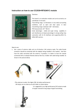


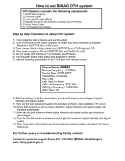
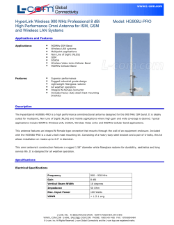
© Copyright 2026