1. technology and computing
2. computer security
3. antivirus and malware

Minimal-MSE linear combinations of variance
estimators of the sample mean
Wheyming Tina Song
Bruce Schmeiser
School of Industrial Engineering
Purdue University
West Lafeyette, IN 47907, U.S.A.
ABSTRACT
All of these methods work well only when underlying assumptions bold. The statistical properties deteriorate as a function of the degree to which
the assumptions are violated. Also, most of the variance estimators have one or two parameters that determine the estimators’ properties. The most common parameter is batch size, which is used by batchmeans and some standardized- time-series estimators. Batch-size estimation based on hypothesis testing has been the classical approach (Bratley, Fox, and
Schrage 1987, Law and Kelton 1983); optimal batch
size in terms of the covariance structure has been recently discussed by Goldsman and Meketon (1986)
and Song and Schmeiser (1988b).
We hope to create an estimator with determined
parameter values that works well for any stationary processes under weak assumptions. Schmeiser
and Song (1987) reported some Monte Carlo results
about linearly combining some known (component)
estimators with low degrees of freedom and creating
a new estimator with more degrees of freedom. Under their assumption that correlations among each
pair of some known estimators are independent of the
underlying process, the linear combinations provide
a better (than the component estimators) estimator
for var(X) without estimating parameter values.
The component estimators in Schmeiser and Song
(1987) have negligible biases, therefore reducing the
variance is the only issue. They consider a vector
of p component estimators, V = (Vˆ1 , Vˆ2 , · · · , Vˆp )with
. The linear comvariance-covariance matrix
V
bination with minimal-variance weights, α =
−1
t
1) retains negligible bias since the
( V−1
1)/(1
V
We continue our investigation of linear combination
of variance-of-the-sample-mean estimator that are
parametered by batch size. First, we state the mseoptimal linear-combination weights in terms of the
bias vector and the covariance matrix of the component estimators for two cases: weights unconstrained
and weights constrained to sum to one. Then we report a small numerical study that demonstrates mse
reduction of about 80% for unconstrained weights
and about 30% for constrained weights. The mse’s
and the percent reductions are similar for all four estimator types considered. Such large mse reductions
could not be achieved in practice, since they assume
knowledge of unknown parameters, which would have
to be estimated. Optimal -weight estimator is not
considered here.
1
INTRODUCTION
Consider a covariance-stationary sequence of random variables {Xi }ni=1 having mean µ, positive variance R0 , and finite fourth moment µ4 . Estimating
var(X), the variance of the sample mean, is a prototype problem in the analysis of simulation output.
Several estimation techniques have been proposed
to estimate var(X), including regenerative (Crane
and Iglehart 1975), ARMA time series models (Fishman 1978, Schriber and Andrew 1984), spectral (Heidelberger and Welch 1981), standardized time series (Goldsman 1984, Schruben 1983), nonoverlapping batch means (Schmeiser 1982), and overlapping
batch means (Meketon and Schmeiser 1984).
1
subject to: αt 1 = 1,
weight are constrained to sum to one.
If estimators do have non-negligible biases, those
optimal-weights yield linear combinations with nonnegligible bias, even though the variance is still minimized, In such case, the linear combination may have
a mean-squared-error (mse), the sum of variance and
squared bias, that is no better than that of some of
the component estimators.
In this paper, we further investigate the idea of
line combinations by no longer restricting the component estimators to negligible bias. The objective is
to form a minimal-mse linear combination by choosing optimal weights. Section 2 is a description of
the minimal-mse problem. Section 3 is a numerical study of linear combinations of nonoverlappingbatch means (NBM), overlapping-batch-means
(OBM), standardized-time-series-area (STS.A), and
the nonoverlapping-batch-means combined with
standardized-time-series-area(NBM+STS.A) estimators. Section 4 is a discussion.
2
where β1 ≥ 0, β2 ≥ 0, and
V
has full rank.
Proposition 1:
For any covariancestationary process X, the optimal solution of (P1) is the minimal-risk linear combination with the weights α =
t −1
(∆−1
1)/(1 ∆ 1) and the resulting miniV
V
mal mse is (1t ∆−1
1)−1 , where ∆V is deV
fined to be β1 ΛV + β2 ΣV .
In our application, bias is defined with respect to
¯
var(X).
We now state three lemmas necessary for proving
Proposition 1. They are proven in Appendices A, B,
and C, respectively.
Lemma 1: (P1) can be written as
(P1’)
minimize: αt ∆V α
subject to: αt 1 = 1
MINTMAL-MSE PROBLEMS
Lemma 2: ∆V in the objective function
of (P1’) is positive definite.
Although we are primarily Interested in mse, we
give optimal weights for the more general risk
β1 bias2 +β2 var, where β1 ≥ 0 and β2 ≥ 0. Mse
corresponds to β1 =1 and β2 =1. We consider two
case constrained and unconstrained. The constrained
case, in which we require the weights to sum to one,
arises naturally when the component estimators are
unbiased. The unconstrained case allows any combinations of weights. These two cases are discussed in
Section 2.1 and 2.2 respectively.
2.1
Lemma 3: Let W be a p × p matrix that
can be decomposed into TTt , where T Is
a nonsingular matrix and let αa be any
p × l scalar vector. Then
(αt Wα) ≥
(αt 1)2
1t W−1 1
Proof of Proposition 1: From Lemma 1, problem
(P1’) and problem (P1) are equivalent, so we focus
on problem (P1’). From Lemma 2 and the Cholesky
decomposition, there exists a nonsingular matrix T
such that ∆V = TTt . Applying the Lemma 3, we
have
(αt 1)2
1
(αt ∆V α) ≥ t −1 = t −1
1 ∆ 1
1 ∆ 1
Constrained Weights
Let V = (Vˆ1 , Vˆ2 , · · · , Vˆp ) be a linearly independent
vector of estimators. Let V be the p × p dispersion
matrix of V , and let ΛV be the p × p matrix with
the (i,j) entry bi bj , where bi ≡bias(Vˆi ). Let αbe a
weighting vector containing p real values αi which is
V
V
the weight associated with Vˆi , used to form a linear sinceαt 1 = 1. Finally, when
combination. The vlue of α then can be chosen to
(∆−1
1)
minimize the risk. This problem can be formulated as
V
α = t −1 ,
(1 ∆ 1)
V
(P1)
minimize: β1 bias2 (αt V ) + β2 var(αt V )
αt ∆V α reaches its lower bound. When both β1 and
β2 are 1, problem (P1) becomes the optimal-mse
2
2.2
problem
In this section, we formulate and solve
minimize: mse(αt V )
(P1.1)
which is (P1) without the constraint on the
We still assume that
weights α.
V has full
rank.Here the optimal linear combination may be biased even when all of the component estimators are
unbiased.
Corollary 1: Problem (P1.1) has optimal
t −1
weights α = (∆−1
1)/(1 ∆ 1) and the
V
resulting minimal mse is ((1t ∆−1
1))−1 ,
V
where ∆−1
is defined to be ΛV + ΣV .
V
Proposition 2.
For any covariancestationary process X, the optimal solution of (P2) is
The special case of (P1.1) with two component estimators is
¯ 1 ξ + β2 Σ )−1 E(V ),
α = β1 var(X)(β
V
V
minimize: mse(α1 V1 + α2 V2 )
(P1.1.1)
where E(V ) is the vector of the
component-estimator means and ξV is
the matrix of cross products of means,
E(V )E(V )−1
subject to: α1 + α2 = 1.
Corollary 2: Problem (P1.1.1) has optimal weights
α1 =
Proposition 2 is obtained by taking first derivatives
after expressing the bias a. the difference of expected
¯
value and var(X).
(α22 + b22 ) − (σ12 + b1 b2 )
(α21 + b21 ) + (α22 + b22 ) − 2(σ12 + b1 b2 )
When both β1 and β2 are 1, problem (P2) becomes the optimal-mse problem
and α2 = 1 − α1 . The resulting minimal
mse is
Corollary 3: Problem (P2.1) has optimal
weights
σ12 ,σ22
are variance of Vˆ1 ,Vˆ2 , and
, where
the covariance of Vˆ1 and Vˆ2 , respectively;
b1 and b2 are bias of Vˆ1 and Vˆ2 , respectively.
¯ + Σ )−1 E(V )
α = var(X)(ξ
V
V
Restriction to two component estimations lead us to
Corollary 2 follows from Corollary 1 by writing
2 + b2
σ
−(σ
+
b
b
)
12
1 2 2
2
−(σ12 + b1 b2 )
σ12 + b21
−1
∆ = 2
2
2
2
V
(σ1 + b1 )(σ2 + b2 ) − (σ12 + b1 b2 )2
(P2.1.1)
minimize: mse(α1 V1 + α2 V2 )
and Corollary 4.
Corollary 4: Problem (P2.1.1) has optimal weights
¯ 1 σ 2 − 2 σ12 )
var(X)(
2
α1 = 2 2
2
1 σ2 + 22 σ12 + σ12 σ22 − 21 2 σ12 − σ12
and
V
minimize: mse(αt V ).
(P2.1)
|(σ22 + b22 ) − (σ12 + b1 b2 )|2
σ22 +b22 − 2
(σ1 + b21 ) + (σ22 + b22 ) − 2(σ12 + b1 b2 )
1t ∆−1
1=
minimize: β1 bias2 (αt V ) + β2 var(αt V )
(P2)
subject to: αt 1 = 1
V
Unconstrained Weights
σ12 + σ22 + b21 + b22 − 2σ12 − 2b1 b2
(σ12 + b21 )(σ22 + b22 ) − (σ12 + b1 b2 )2
and
Alternatively Corollary 2 can be obtained directly by
taking first derivatives.
α2 =
¯ 2 σ 2 − 1 σ12 )
var(X)(
1
2
21 σ22 + 22 σ12 + σ12 σ22 − 21 2 σ12 − σ12
where 1 and 2 are the expected value of
V1 and V2 , respectively.
3
3
values of mse(V (m∗ )) shown in the last row, is
NBM+STS.A, NBM, OBM, and STS.A. which differs
from the results in Song and Schmeiser (1988b) where
the order is OBM, NBM, NBM+STS.A, and STSA
for the same process and n=500. We emphasize this
difference to discourage the reader from making type
comparison. based on the Insufficient information in
this study. Our only current purpose is to demonstrate mse-reduction with linear combinations.
NUMERICAL STUDY
The objective of the numerical study in this section
is to see how much the use of linear combinations
can Improve (reduce) the e and to study bow the optimal component estimators behave as a function of
estimator type, batch size, and statistical properties
(bias, variance, and mse).
Specifics of the study are as follows. The component estimators are NBM, OBM, STS.A, and
NBM+STS.A. The sample size n is 30. The data process is steady-state first-order autoregressive (AR(1))
with the parameter φ1 =0.8082. This value of φ1 , cor
responds to γ0 ≡ ∞
h=−∞ ρh =10 , where ρh denotes
the lag-h autocorrelation corr(Xi , Xi+h ), The arbi¯ The biases, varitrarily value 1 is used for var(X).
ances, and mse’s are calculated numerically, using the
approach discussed in Song and Schmeiser (l988a).
Before considering linear combinations in Section
3.2, we investigate the optimal mse for individual
component estimators in Section 3.1.
3.1
3.2
In this section we numerically demonstrate the msereduction obtained with linear combinations of two
component estimators for the sample size and process
described in Section 3.1 The minimal-mse problems
considered are (P1.1.1), weights constrained to sum
to one, and (P2.1.1), unconstrained weights. The numerical results for these two problems, are discussed
in Section 3.2.1 and Section 3.2.2, respectively.
In each linear combination, let V (m1 ) and V (m2 )
denote the two component estimators with batch size
m1 and m2 , respectively. Let V ∗ ≡ α∗1 V1 (m∗1 ) +
α∗2 V2 (m∗2 ) denote the mse-optimal linear combination
of V (m1 ) and V (m2 ) with corresponding weights α∗1
and α∗2 and corresponding optimal batch size m∗1 and
m∗2 .The weights and batch size. are simultaneously
optimal in the sense that for any values of α1 , α2 ,
m1 , and m2
Optimal Mse: Component Estimators
For the four component estimator types, we numerically compute their optimal batch sizes and optimal mse’s, as well as associated biases and variances.
These statistical properties are reported here primarily for comparison to the statistical properties of the
linear combinations studied in Section 3.2. Coldsman
and Meketon (1986) and Song and Schmeiser (1988b)
contain a more complete study of the four component
estimator types for this process.
Let m denote the batch size and V (m) denote the estimator type of NBM, OBM, STS.A,
and NBM+STS.A with batch size m.
Let
m∗ denote the mse-optimal batch size; i.e.
mse(V (m∗ )) ≤mse(V (m))for all batch size m. Th.
numerically determined optimal batch else, squared
bias, variance, and mse for V (m∗ ) of the four estimator type. are shown in Table 1.
mse(V ∗ )≡mse(α∗1 V1 (m∗1 ) + α∗2 V2 (m∗2 ))
≤mse(α1 V1 (m1 ) + α2 V2 (m2 ))
The values of squared bias, variance, covariance, and
mse in Table 2 through Table 4 are multiplied by 102
because some values are very small.
3.2.1
NBM
OBM
STS.A
NBM+STS.A
7
33.6
13.7
47.3
8
33.6
14.1
47.7
15
39.3
15.0
54.3
15
28.9
16.6
45.5
Constrained Weights Summing to One
Consider the minimal-mse problem (P1.1.1) where
the optimal weights sum to one. In this section we
use α and 1 − α rather than α1 and α2 , since the constraint makes this an inherently one-weight problem.
The component estimators to be combined can be of
common type or of different types. The results of
combining common types are shown in Table 2 and
different types in Table 3.
In Table 2 we combine common types of estimators (with different batch sizes), allowing us to
Table 1: Optimal Batch Size and Their Properties
Property
Estimator Type
m∗
2
bias (V (m∗ )) × 102
var(V (m∗ )) × 102
mse(V (m∗ )) × 102
Optimal Mse: Linear Combinations
The order of the estimator types in increasing
4
temporarily drop the subscript on V
Properties
Song (1987), where the linear combinations considered resulted in variance decreases that were similar
Table 2: Optimal Linear Combination:
across types of estimators.
Common Types of Component Estimators.
Optimal Weights Summing to One.
To provide some insight into the nature of the perProperty
Estimator Type
formance of the optimal linear combination compared
NBM
OBM
STS.A
NBM+STS.A
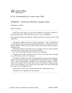
to that of component estimators, consider Figure 1,
(m∗1 , m∗2 )
(1, 2)
(1, 2)
(2, 5)
(2, 3)
2
∗
2
which shows the statistical properties (bias, variance,
bias (V (m1 )) × 10
82.9
82.9
95.7
82.9
bias2 (V (m∗2 )) × 102
70.3
70.5
83.4
76.0
and mse) of the NBM estimators corresponding to
var(V (m∗1 )) × 102
0.227
0.227
0.00643
0.227
various batch sizes and of the optimal linear combivar(V (m∗2 )) × 102
0.940
0.935
0.272
0.525
∗
∗
2
(m ), V
(m )) × 10
nation. The small variances and large biases associcov(V
0.460
0.458
0.0112
0.345
1
2
corr(V (m∗1 ), V (m∗2 ))
0.996
0.996
0.268
0.999
ated with batch sizes m∗1 =1 and m∗2 =2 , which are
α∗
-7.25
-7.33
-8.37
-15.0
used in the optimal linear combination, are shown on
1 − α∗
8.25
8.33
9.37
16.0
the left side of the figure. The squared bias, variance,
bias2 (V ∗ ) × 102
9.80
10.3
13.7
8.45
∗
2
var(V ) × 10
20.9
21.1
22.6
20.1
and mse of the optimal linear combination are shown
mse(V ∗ ) × 102
30.7
31.4
36.2
28.6
as horizontal lines through the figure. We see that
∗)
mse(V
1−
35%
34%
33%
37%
∗
mse(V (m ))
in addition to the 35% mse reduction, the bias is less
than the bias of NBM with any batch sue and the
Now observe the individual component estimators variance is less than NBM variances for batch sizes
that comprise the optimal linear combinations in Ta- greater than seven. Although not shown, the analble 2. The optimal pairs of batch size m∗1 and m∗2 ogous figures for OBM, STS.A, and NBM+STS.A
have relative small values, as shown in the first row. show similar results.
Such batch sues correspond to large biases, as shown
in the second and third rows; and small variances, as
AR(1), γ0=10, n=30
shown in the fourth and filth rows.
1.00
mse(Vˆ)
0.90
Now observe the relationships among the comvar(Vˆ)
0.80
ponent estimators that comprise the optimal linear
0.70
combinations. The covariances and correlations of
0.60
the two optimal component estimators, shown in the
0.50
sixth and seventh rows, are positive. Except for the
0.40
STS.A estimator, the correlations are close to one.
mse(Vˆ * )
0.30
The optimal weights α∗ and 1-α∗ have different
var(Vˆ * )
0.20
bias 2(Vˆ)
signs, which both partially cancels the large biases of
0.10
bias 2 (Vˆ * )
the two component estimators and uses the positive
0.00
correlation to obtain small variance. These effects
1 2 3 4 5 6 7 8 9 10 11 12 13 14 15
batch size m
can be seen in the formulas for the bias and variance
of the linear combination, which are
Figure 1: Statistical Properties of the NBM Estimators
bias(V ∗ )=α∗ bias(V1∗ )+(1-α∗ )bias(V2∗ )
and of the Optimal Linear Combination
and
var(V ∗ )=(α∗ )2 var(V1∗ )+(1 − α∗ )2 var(V2∗ )
+2α∗ (1-α∗ )cov(V1∗ ,V2∗ )
Table 3 is similar to Table 2, except that it
contains the results for linear combinations composed of two different types of component estimators. The second, third and fourth columns of Table
3 show results for the linear combinations of (NBM,
STS.A), (OBM, STS.A) and (NBM, OBM), respectively. Again, we see that the batch sizes in the optimal linear combination are small, with corresponding
Now observe the mean squared error. Comparing
mse(V ∗ ) to mse(V (m∗ )), which is obtained in Section
3.1, we see the mse-reduction is about 35% for any
of the four estimator types. This consistency across
types of estimators is reminiscent of Schmeiser and
5
the optimal linear combination for common component types In Table 4.
The batch sizes m∗1 and m∗2 shown in the first row
are again small. These batch sizes still correspond to
large biases and small variances.
The optimal weights α∗1 and α∗2 do not sum to
one. For the first time, we see an example where
the signs are both positive–STS.A. The bias of the
optimal linear combination is
large biases and small variances. The covariances and
correlations of the two component estimators are positive. The optimal weights α∗ and 1-α∗ have different signs, again allowing the biases to partially cancel
and the variance to be small. The mse-reduction is
about 30% compared to mse(VN BM +ST S.A (m∗ )) from
Table 2. We use VN BM +ST S.A (m∗ ) as the basis to
compute the mse reduction because it has the smallest mse in the last row of Table 1.
3.2.2
bias(V ∗ )=α1 bias(V1 )+α2 bias(V2 )
¯
+(α1 + α2 − 1)var(X)
Unconstrained Weights.
Consider the minimal-mse problem (P2.1.1). Since
Because of the last term, the signs of the optithe optimal weights are unrestricted, the mse(V ∗ )
must be smaller than or equal to the optimal mse’s mal weights need not be different for the biases to
partially offset each other.
obtained in Section 3.2.1.
The bias2 , var, and mse shown in the fourth-toTable 3: Optimal Linear Combination:
last, third-to-last, and next-to-last row, respectively,
Different Component Estimators Types.
are much smaller than the corresponding values in
Optimal Weights Summing to One.
Table 2. The mse reduction is about 80%, which is
Property
Estimator Types (V1 , V2 )
(NBM,STS.A)
(OBM,STS.A)
(NBM+OBM)
far larger than 35% in the last row of Table 2 and the
(m∗1 , m∗2 )
(2, 2)
(1, 2)
(1, 2)
30% in the last row of Table 3.
2 ∗
2
bias (V (m1 )) × 10
bias2 (V (m∗2 )) × 102
var(V (m∗1 )) × 102
var(V (m∗2 )) × 102
(m∗ ), V
(m∗ )) × 102
cov(V
1
2
corr(V (m∗1 ), V (m∗2 ))
α∗
70.2
95.7
0.940
0.00643
0.0114
0.147
82.9
95.7
0.227
0.00643
0.00882
0.231
82.9
70.5
0.227
0.935
0.458
0.996
4
DISCUSSION
We have given formulas for mse-optimal linear combinations and numerically studied estimator perfor4.75
9.83
-7.33
mance for a particular AR(1) process. The formulas,
1 − α∗
-3.75
-8.83
-8.33
bias2 (V ∗ ) × 102
9.83
9.87
10.3
which are functions of the biases, variance., and covar(V ∗ ) × 102
20.9
20.9
21.1
variances of the component estimator,, consider the
mse(V ∗ ) × 102
30.7
30.8
31.4
∗)
mse(V
constrained and unconstrained cases. The numerical
1−
33%
32%
31%
N BM +ST S.A (m∗ ))
mse(V
study demonstrated mse reductions of about 30% for
Table 4: Optimal Linear Combinations:
all constrained linear combination, and about 80%
Common Component Estimators Types.
for all unconstrained linear combinations.
Unconstrained Weights.
The various estimator types all lead to simiProperty
Estimator Type
NBM
OBM
STS.A
NBM+STS.A
lar optimal mse’s. The tentative conclusion is that
(m∗1 , m∗2 )
(1, 3)
(1, 2)
(2, 3)
(2, 5)
the choice of component estimator type is relatively
bias2 (V (m∗1 )) × 102
82.9
82.9
95.7
82.9
unimportant.
bias2 (V (m∗2 )) × 102
59.9
70.5
92.2
58.8
var(V (m∗1 )) × 102
0.227
0.227
0.00643
0.227
In practice, the variance of the sample mean, the
var(V (m∗2 )) × 102
21.8
0.935
0.0327
1.54
bias vector, and the covariance matrix are unknown.
(m∗ ), V
(m∗ )) × 102
cov(V
0.696
0.458
0.00568
0.588
1
2
Estimation of the batch sizes and optimal weights,
corr(V (m∗1 ), V (m∗2 ))
0.990
0.996
0.392
0.995
∗
which is not studied here, may be difficult. We do not
α
39.2
56.2
27.8
51.3
∗
1−α
-11.5
-25.8
7.44
-18.4
yet know the relative difficulties of estimating batch
bias2 (V ∗ ) × 102
0.98
1.06
1.03
0.827
sizes for component estimator, single weights for convar(V ∗ ) × 102
8.92
9.25
9.11
8.27
∗
2
strained linear combinations, and double weights for
mse(V ) × 10
9.90
10.3
10.1
9.09
∗)
mse(V
unconstrained linear combinations. Therefore, the
1−
79%
78%
81%
80%
(m∗ ))
mse(V
extent to which we can benefit from the mse reducUsing the same proc and sample size, we show tions demonstrated here is unknown.
6
β1 bias2 (αt V )= β1 (αt bbt α)
=β1 (αt ΛV α)
=αt (β1 ΛV )α
Some results necessary for estimating properties
of component estimator are available. Schmeiser and
Song (1987) discuss correlations among estimators
with large batch size and hypothesize that the asymptotic correlations are not a function of the process and
are good approximations for even small sample uses.
Goldsman and Meketon (1988) and Song and Scbmeiser (1988b) discuss optimal batch sizes for component estimators. The component estimator S 2 /n;
which is NBM with batch size one, OBM with batch
size one, or NBM+STS.A with batch size 2; arises
repeatedly in numerical results and has easily computed bias (e.g., David (1985)). We know of no other
component estimator with known bias.
Keep in mind that the numerical results are for
a single sample size and process. The sample size is
quite small; n= 30 is only three times the sum of the
correlations γ0 =10. However, the example reported
is consistent with a limited amount of other experience, so we think the example is not misleading. The
small sample size was used because (1) it allowed numerical (rather than Monte Carlo) mse calculations
and (2) our experience indicates that even such a
small sample size yield results consistent with large
sample sizes. Nevertheless, results should be extrapolated only with caution. All that can be claimed with
certainty is that this one example has demonstrably
large potential mse reduction.
Also
β2 var(αt V ) =β2 (αt V α)
=αt (β2 V )α
Therefore
β1 bias2 (αt V )+ β2 var(αt V ) =αt [β1 ΛV + β2
=αt ∆V α ]α
V
APPENDIX B: PROOF OF LEMMA 2
We show that the objective function of (P1’),
∆V ≡ β1 ΛV + β2 V , is positive definite , where
β1 ≥ 0 and β2 > 0.
By definition, ΛV ≡bbt , where b=[b1 , b2 , · · · , bp ]t ,
and
t
≡E{[V −E(V )][V −E(V )] }
V
For any nonzero real vector s,
st ∆V s = st (β1 ΛV + β2 ΣV )s
= st (β1 ΛV )s + st (β2 ΣV )s
= β1 (st bbt s) + β2 E{st [V − E(V )][V −
E(V )]t s}
ACKNOWLEDGMENT
= β1 (st b)2 + β2 E{[st (V − E(V ))]2 } > 0,
This material is based upon work supported by the
National Science Foundation under Grant No. DMSsince β1 ≥ 0; (st b)2 ≥ 0; β2 ≥ 0; and since ΣV
8717799. The Government has certain rights in this has full rank, which implies that st (V −E(V )) = 0,
materiel.
therefore, E{[st (V −E(V ))]2 } > 0. So, ∆V is positive
definite.
APPENDIX A: PROOF OF LEMMA 1
Define bias(V ) to be the bias vector, b = (b1 , · · · , bp )t ,
APPENDIX C: PROOF OF LEMMA 3
¯ Then
where bi ≡ bias(Vi ) ≡ E(Vi )-var(X).
t 1 − 1)
¯
bias(αt V )=αt b +var(X)(α
(αt 1)2 = (αt I1)2
= (αt (TT−1 )1)2
=αt b
= [(αt T)(T−1 1)]2
since
αt 1=1.
≤ (αt T)(αt T)t(T−1 1)t (T−1 1)
t
Let ΛV ≡ bb . Then
t
t
t
= (α TT α)(1 ((T
t
t
= (α Wα)(1 W
7
−1
−1 t
1)
)T
−1
(A.C.1)
)1)
(A.C.2)
Inequality (A.C.1) follows by applying the [10] Schmeiser, B. (1982). Batch-size effects in the
analysis of simulation output. Operations ReCauchy-Schwartz Inequality (X t Y )2 ≤ (X t X)(Y t Y )
search 30, 556-568.
. From (A.C.2) we have
(αt 1)2 = (αt Wα)(1t W−1 1),
[11] Schmeiser, B. and Song, W.-M.T. (1987). Correlation among estimators of the variance of the
sample mean. In:Proceedings of the 1987 Winter
Simulation Conference(A. Thesen, H. Grant, W.
David Kelton, eds.), 309-316.
which implies
(αt Wα) ≥
(αt 1)2
.
(1t W−1 1)
[12] Schriber, T.J. and Andrews, R.W. (1984).
ARMA-based confidence interval procedures for
[1] Bratley, P., Fox. B.L. and Schrage, 1.. (1987). A
simulation output analysis. American Journal of
Guide to Simulation. Springer-Verlag.
Mathematical and Management Science 4, 345373.
[2] Crane, MA. and Iglebart, D.L. (1975). Simulating stable stochastic systems, m: regenerative [13] Schruben, LW. (1983). Confidence interval esprocess and discrete-event simulations. Operatimation using standardized time series. Operations Research 23, 33-45.
tions Research 31, 1090- 1108.
REFERENCE
[3] David, HA. (1985). Bias of S 2 under depen- [14] Song, W.-M.T. and Schmeiser, B. (1988a). Estidence. American Statistician 39, 201.
mating variance of the sample mean: quadraticforms and cross-product, covariances. Opera[4] Fishman, G.S. (1978). Grouping observations in
tions Research Letters 7(1988a), in press.
digital simulations. Management Science24, 510521.
[15] Song, W.-M.T. and Schmeiser, B. (1988b). Estimating standard errors: Empirical behavior of
asymptotic mse optimal batch sizes. In: 20th
Symposium on the Interface: Computing Science
and Statistics, forthcoming.
[5] Goldsman, D. (1984). On using standardized
time series to analyze stochastic process. Ph.D.
Dissertation, School of Operations Research
and Industrial Engineering, Cornell University,
Ithaca, New York.
AUTHOR’S BIOGRAPHIES
[6] Goldsman, D. and Meketon, M. (1986). A comparison of several variance estimators. Technical
Report J-85-12, Department of Operations Research, AT&T Bell Laboratories, Holmdel, NJ
07733.
Wheyming Tina Song Is a Ph.D. candidate in the
School of Industrial Engineering at Purdue University, majoring In simulation and applied probability.
She received her undergraduate degree In statistics
and master’s degree in industrial management at
[7] Heidelberger. P. and Welch, PD. (1981). A spec- Cheng-Kung University in Taiwan. She then retral method for confidence interval generation ceived her master’s degrees in applied mathematics
and run length control in simulation. Communi- and industrial engineering from the University of
cation, of the ACM 24, 233-245.
Pittsburgh.
[8] Law, AM. and Kelton, W.D. (1983). Simulation
Wheyming Tina Song
Modeling and Analysis. McGraw-Hill.
School of Industrial Engineering, Purdue University
[9] Meketon, M.S. and Schmeiser, B. (1984). Over- West Lafayette, IN 47907, U.S.A.
lapping batch means: something for nothing? (317) 743-8275
In: Proceedings of the 1984 Winter Simulation [email protected] (arpanet)
Conference (S. Sheppard, U. Pooch, acid D. Pegden, ed.), 227-230.
8
Bruce Schmeiser is a professor in the School of Industrial Engineering at Purdue University. He received
his undergraduate degree in mathematical sciences
and master’s degree in industrial and management
engineering at The University of Iowa. His Ph.D.
is from the School of Industrial and Systems Engineering at the Georgia Institute of Technology. He
is the Operations Research area editor in simulation
and has served in editorial positions of IIE Transactions, Communications in Statistics, B: Simulation
and Computation, Journal of Quality Technology,
American Journal of Mathematical and Management
Sciences, and the handbook of Industrial Engineering. He is the past chairman of the TIMS College
on Simulation and Gaming. He represents ORSA
on the Winter Simulation Conference Board of Directors, currently serving as chairman. His research
interest. are the probabilistic and statistical aspects
of digital-computer stochastic simulation, including
input modeling, random-variate generation, output
analysis, and variance reduction.
Bruce Schmeiser
School of Industrial Engineering
Purdue University
West Lafayette, IN 47907, U.S.A.
(317) 494-5422
[email protected] (arpanet)
9