Joint-layer Encoder Optimization for HEVC Scalable Extensions
Chia-Ming Tsai, Yuwen He, Jie Dong, Yan Ye, Xiaoyu Xiu, Yong He
InterDigital Communications, Inc., 9710 Scranton Road, San Diego, CA 92121, USA
ABSTRACT
Scalable video coding provides an efficient solution to support video playback on heterogeneous devices with various
channel conditions in heterogeneous networks. SHVC is the latest scalable video coding standard based on the HEVC
standard. To improve enhancement layer coding efficiency, inter-layer prediction including texture and motion
information generated from the base layer is used for enhancement layer coding. However, the overall performance of
the SHVC reference encoder is not fully optimized because rate-distortion optimization (RDO) processes in the base and
enhancement layers are independently considered. It is difficult to directly extend the existing joint-layer optimization
methods to SHVC due to the complicated coding tree block splitting decisions and in-loop filtering process (e.g., deblocking and sample adaptive offset (SAO) filtering) in HEVC. To solve those problems, a joint-layer optimization
method is proposed by adjusting the quantization parameter (QP) to optimally allocate the bit resource between layers.
Furthermore, to make more proper resource allocation, the proposed method also considers the viewing probability of
base and enhancement layers according to packet loss rate. Based on the viewing probability, a novel joint-layer RD cost
function is proposed for joint-layer RDO encoding. The QP values of those coding tree units (CTUs) belonging to lower
layers referenced by higher layers are decreased accordingly, and the QP values of those remaining CTUs are increased
to keep total bits unchanged. Finally the QP values with minimal joint-layer RD cost are selected to match the viewing
probability. The proposed method was applied to the third temporal level (TL-3) pictures in the Random Access
configuration. Simulation results demonstrate that the proposed joint-layer optimization method can improve coding
performance by 1.3% for these TL-3 pictures compared to the SHVC reference encoder without joint-layer optimization.
Keywords: Video coding, scalable video coding, joint-layer optimization, rate-distortion optimization
1. INTRODUCTION
With advances in computer networks, more efficient multimedia compression technologies, and more mature multimedia
streaming technologies [1], people can access multimedia content more conveniently than ever. Multimedia content
delivery has migrated from a server-client based solution to a CDN-based solution. With video streaming, the
multimedia content may be transmitted through heterogeneous environments and may be adapted to the display
capabilities of various playback devices [2]. To this end, scalable video coding provides an efficient and attractive
solution for universal video access [3] from different kinds of devices. With scalable video coding, a generic scalable
video bitstream can contain multiple representation layers, in which one is the base layer to provide basic video quality
and the others are enhancement layers to support various adaptations, such as view, spatial, temporal, fidelity and color
gamut scalabilities. For example, the server can dynamically decide the subset of layers to be transmitted or the client
can dynamically decide the subset of layers to request based on available resources including network condition, the
client’s battery, CPU status, etc.
Scalable video coding technology has been adopted in many existing video coding standards [4][5]. In H.264/AVC,
scalable video coding referred to as SVC is an extension (Annex G) of the single layer video coding standard [5]. In
order to support various video adaptation requirements, SVC adopts several inter-layer prediction tools such as interlayer mode prediction, inter-layer motion prediction and inter-layer residual prediction, to reduce information
redundancy between enhancement layers and the base layer [6]. One important feature of SVC known as single-loop
decoding (SLD) allows the SVC decoder to utilize only one motion compensation prediction (MCP) and deblocking
loop to reconstruct a higher layer, without completely reconstructing pictures of lower dependent layers. Therefore, it
reduces the computation resources and memory access bandwidth requirements at the decoder side. Because the
restricted intra prediction constraint is applied at lower layers in order to support SLD, overall coding efficiency of SVC
is reduced to some extent.
After completing the first version of the High Efficiency Video Coding (HEVC) standard [7], ITU-T VCEG and
ISO/IEC MPEG jointly issued the call for proposals for the scalable extension of the HEVC standard [8] (also known as
SHVC). Unlike SVC, which is based on block level inter-layer prediction design, SHVC is developed by changing high
level syntax to achieve various video scalability requirements [9]. Such high level syntax-based design applies an interlayer prediction process to lower layer reconstructed pictures to obtain the inter-layer reference pictures. Then, to predict
higher layer pictures, the inter-layer reference pictures are used as additional reference pictures without resorting to
block level syntax changes. Compared to prior scalable video coding standards, SHVC can be more easily implemented
as the overhead of architecture design changes is largely reduced. Another feature of SHVC is hybrid scalable coding,
which allows the base layer pictures to be coded using a legacy standard such as H.264/AVC or MPEG-2. The hybrid
scalability feature can provide efficient video services to users with legacy devices and users with new devices
simultaneously. Color gamut scalability is another new functionality of SHVC, which supports efficient scalable coding
when different color spaces are used in the base and enhancement layers.
In the SHVC reference encoder [14], layers are coded independently. In the reference encoder, a first coding loop is used
to encode and output the base layer bitstream. Then, the inter-layer prediction process is applied to the reconstructed
base layer picture. Finally, a second coding loop is used to encode and output the enhancement layer bitstreams. As such,
the rate-distortion optimization (RDO) decision in each layer is performed independently. Without joint layer
optimization, the scalable coding efficiency is not optimal, especially when compared to the single layer coding
efficiency [10]. To improve the coding efficiency of scalable video coding, several joint-layer optimization methods
have been previously proposed [11][12]. Although these methods show significant coding performance improvement, it
is hard to directly apply them to SHVC due to complicated CTU splitting decision and in-loop filtering process (e.g. deblocking and SAO filtering) in HEVC encoding. Besides, when the network bandwidth fluctuates, the user side cannot
always be guaranteed to receive the best quality video layers, and may receive lower quality layers when bandwidth is
reduced. Therefore, the joint-layer optimization method should consider the video quality variation to ensure optimal
video quality at the user side. To solve these problems, we propose a joint-layer optimization method that adjusts QP to
allocate the bit resource between layers and considers the viewing probability of base and enhancement layers to
optimize the encoding control.
The rest of this paper is organized as follows. In Section 2, we review the related joint-layer optimization methods.
Section 3 presents the proposed joint-layer optimization method for SHVC and the viewing-probability-based quality
metric, respectively. Section 4 reports the experimental results. Finally, conclusions are drawn in Section 5.
2. RELATED WORK
To improve the scalable video coding performance, several joint-layer optimization methods for scalable video coding
were previously proposed [11][12]. In [11], an RD optimized multi-layer encoder control method was developed to
jointly consider the coding impact of each layer. When performing mode decision, deriving motion vector and selecting
the transform coefficient levels, these coding parameters of base and enhancement layers are jointly decided. The bit rate
of scalable coding increase can be reduced to as low as 10% when compared to single layer coding (H.264) at high
spatial resolution (4CIF). In comparison, the bit rate increase is about 15~20% using non-optimized SVC. In [12], a onepass multi-layer encoder control method for quality scalability is proposed. Similar to the method in [11], the method in
[12] simplifies the mode decision process by assuming the mode decision results in the base layer and the enhancement
layers are the same. Therefore, it is not required to evaluate all possible coding parameter combinations in base and
enhancement layers for quality scalable coding.
The existing joint-layer optimization methods use the Lagrangian approach [13] to allocate the bit resources between
base and enhancement layers. As formulated in (1), the coding parameters of the base layer, , are determined by:
{
}
(
)
(
),
(1)
where is the Lagrange multiplier, ( ) and ( ) are the corresponding distortion value and the rate of the base layer,
respectively. Similarly, the coding parameter of the i-th enhancement layer, , can be formulated as:
{ |
}
( |
)
( ( |
)).
(2)
When only a two-layer scenario is considered, the joint decision of the coding parameters in the base and enhancement
layers is formulated as:
{
|
}(
)(
(
)
(
))
(
(
|
)
(
(
)
(
|
))),
(3)
where is the weighting value to control the trade-off of coding efficiency between the base and enhancement layers. If
is set to 0, then the joint-layer encoder control process is only optimized for the base layer. On the contrary, if is set
to 1, then only the enhancement layer is optimized given the base layer coding parameters p0.
It is difficult to directly extend the existing joint-layer optimization methods to SHVC for the following three reasons:
1.
For the method in [11], the coding mode decision for the base layer and enhancement layers are jointly determined.
However, because the block partition method in HEVC is quad-tree based design, joint optimization of base and
enhancement layer coding modes will result in too many combinations.
2.
The process of coding mode decisions in HEVC is a recursive process. If the method in [11] is extended to SHVC, it
will require a lot of memory to store all the recursive call stacks.
3.
In SHVC, HEVC in-loop filtering processes, e.g., de-blocking and SAO filtering, are supported. These in-loop
filtering processes in the reference encoder are applied at slice level. It is difficult to do optimal joint-layer mode
decisions at the CU level, as the slice level in-loop filtering processes can invalidate the optimal mode decision
made at the CU level. Further, the upsampling process used to generate the inter-layer reference picture is applied
on the base layer reconstructed picture, which makes block-level joint-layer optimization difficult.
To avoid the aforementioned issues, we propose a joint-layer optimization method that adaptively adjusts the QP value
of each CTU to control the bit resource allocation. The proposed method also considers the joint viewing probability of
the base and enhancement layers. The detailed proposed method will be presented in Section 3.
3. THE PROPOSED JOINT-LAYER OPTIMIZATION METHOD
3.1 Optimal QP pair selection
To avoid the difficulties caused by a complicated CTU splitting decision and in-loop filtering process, the proposed
joint-layer optimization method applies CTU-level QP control in the base layer to adjust the bit resource between base
and enhancement layers. Let us denote a CTU as a referenced CTU (r-CTU) if and only if at least one of CUs within the
CTU is referenced by the higher layer, and denote a CTU as a non-referenced CTU (nr-CTU) otherwise.
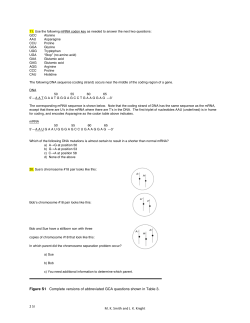
As shown in Figure 1, the proposed method is a 2-step process:
1.
The first step records the inter-layer reference (ILR) relations between layers. The base and enhancement layers of
the current picture are encoded without changing the QP. Then, the CTUs in lower layer are classified into r-CTUs
and nr-CTUs. The reference relations will be used in the second step.
2.
In the second step, a pair of QPs consisting of
for r-CTUs and
for nr-CTUs, are selected for each picture
to optimize the bit resource allocation. The QP of r-CTUs is decreased by
to improve the quality of those rCTUs for improved ILR prediction performance, and the QP of nr-CTUs is increased by
to save more bit
resource for the r-CTUs.
To clearly explain the operations in the second step, denote the current picture as , where i is the frame number and t is
the corresponding temporal level. To adjust the QP of r-CTUs and nr-CTUs in the base layer of , let
{
} {(
)(
)
(
)} denote a
QP list with n QP pairs for the t-th temporal level. For the k-th QP pair (i.e.,
),
and
denote the delta QPs for the r-CTUs and nr-CTUs, respectively. In other words, if the QP of the base layer at
the t-th temporal level is
, then the k-th QP pair for the r-CTUs and nr-CTUs are (
) and (
), respectively. Each layer will be encoded n times to find the best QP pair for coding each layer of .
3.2 Viewing-probability-based bit allocation
Network bandwidth fluctuation often causes packet loss. Therefore, it is hard to guarantee that the user side can always
completely receive the highest quality layers. In this paper, we consider the network environment scenario when
designing the joint-layer optimization method. Assume the output bitstream uses hierarchical B coding structure and
contains two layers with the same frame rate but possibly the same or different spatial resolutions. When network
bandwidth fluctuates, some enhancement layer data from the video frames with the highest temporal level will be
dropped first. In this case, the user will be watching lower quality or upsampled lower resolution base layer pictures at
these time instances.
Input Video
Collect ILR statistics
Set QP pair
Is a referenced CTU?
Yes
Decrease QP value
No
Increase QP value
No
Update the λ value for RDO
process by the new QP value
Encode base/enhancement layer
pictures and record RD statistic
Is the last QP pair?
Yes
Output the AU with the best QP
pair settings
Bitstream
Figure 1. The proposed joint-layer optimization method for SHVC.
To maximize the user’s viewing experience and make the resource allocation more reasonable, the proposed joint-layer
optimization method considers the viewing probability of base and enhancement layers in the RD decision function by
defining the RD cost of
as:
(
)
(
(
) (
)
(
)
)
(
(
)
(
)),
(4)
( ) and
( ) are the distortion values of the base and enhancement layers,
( ) and
( ) are the rate of
where
the base and enhancement layers, is the viewing probability of enhancement layer,
is the lambda value for the
mode decision process of enhancement layer at the t-th temporal level, and
is the weight value to control the coding
efficiency trade-off between layers. If the base and enhancement layer data of the t-th temporal layer are fully received
(i.e., is assigned to 1), then the RD cost function in (4) can be formulated as in (5), and it optimizes only the
enhancement layer quality.
(
Finally, the best QP pair for
)
(
)
is selected by:
(
(
)
(
)).
(5)
(
).
(6)
The coded NAL units of each coding loop are temporarily stored, and then the access unit coded by using the best QP
pair is chosen and written to the output bitstream.
3.3 Viewing-probability based quality metric
As aforementioned, due to the packet loss caused by fluctuating network bandwidth, the user side may not always enjoy
high quality videos. Instead, with scalable video coding, the video quality would be adjusted dynamically. Therefore,
only the Peak Signal-to-Noise Ratio (PSNR) of the enhancement layer video or only the PSNR of the base layer video is
not an appropriate measurement of the end user’s experience. A more proper quality measurement metric needs to
jointly consider the viewing probability of base and enhancement layers at the user side. To this end, we define a new
quality measurement method based on the viewing probability.
As formulated in (7), the traditional PSNR calculation method is defined as
(7)
where
is the maximum pixel value,
is the video frame size, and
original frame and the reconstructed frame. The
term can be rewritten as
(
is the sum of squared error between the
(8)
)
To take into account viewing probability, the
term in (7) is modified as the linear combination of the
values of
the corresponding pictures in the base and enhancement layers. The new PSNR calculation method is defined as
(
(
)
((
where the viewing probability of base and enhancement layers are (
of the corresponding pictures in the base and enhancement layers.
(9)
)
)
) and ,
(
)
and
)
are the
values
4. EXPERIMENTAL RESULTS
The proposed joint-layer optimization method is implemented based on the SHVC reference software SHM-2.0 [14].
The coding parameters are configured based on the SHVC common test conditions (CTC) [15]. Three test sequences,
Kimono, Cactus and BaseketballDrive, are used in the simulations. The experiments are evaluated under the “Random
Access” coding structure, and the spatial scalability is set to 2X. SHVC CTC defines two QP sets for coding base and
enhancement layers. To evaluate the performance of the proposed method, the performance of SHM-2.0 is chosen as the
anchor, and Bjøntegaard Delta (BD) rate [16] is used as the evaluation metric for comparison with anchor.
In the experiments, we assume the user side has an 80% probability of receiving the enhancement layer data of the
highest temporal level (i.e., is set to 0.8 when temporal level is 3), and the other temporal layer data are fully received.
Therefore, for the third temporal level, the proposed method uses equation (4) as the RD cost function, and equation (9)
is used as the quality measurement metric. For the other temporal levels, equation (5) is used as the RD cost function,
and the quality metric is equation (7). Additionally, the weighting values for the highest temporal level are set to 1.2, and
for the other temporal levels are set to 1.4 (i.e.,
,
). For the QP pair settings, the delta QPs
for the third temporal level pictures are {0, 2, 4, 6}, i.e., the QP pairs are (0, 0), (0, 2), … , (6, 4), (6, 6). For the first and
second temporal levels, the delta QPs are chosen from {0, 1, 2, 3}, i.e., the QP pairs are (0, 0), (0, 1), … , (3, 2), (3, 3).
For the lowest temporal level, the delta QPs for nr-CTUs are not changed, and the QP pairs are (0, 0), (1, 0), (2, 0), and
(3, 0), respectively.
Table 1. Overall BD-rate results of the proposed joint-layer optimization method compared with SHM-2.0. For the
third temporal level, the viewing probability of the enhancement layers is set to 0.8, and the quality is measured by
(9).
Seq.
QPI QPI
Base Enh.
SHM-2.0
kbps
Proposed Method
Y psnr U psnr V psnr
kbps
BD-rate (Proposed vs. SHM)
Y psnr U psnr V psnr
22
22
5433.42
41.25
43.18
44.73
5412.51
41.24
43.19
44.75
26
26
2838.77
39.75
41.98
43.23
2830.07
39.76
41.99
43.25
30
30
1592.18
37.98
41.08
42.25
1588.26
38.00
41.09
42.25
34
34
897.02
36.03
40.06
41.25
894.00
36.04
40.06
41.25
22
24
3741.15
40.58
42.59
43.94
3765.15
40.59
42.59
43.96
26
28
2009.75
38.89
41.44
42.59
2016.12
38.91
41.45
42.61
30
32
1117.22
36.98
40.50
41.65
1113.74
36.99
40.51
41.65
34
36
663.34
35.10
39.75
40.97
660.21
35.11
39.76
40.99
22
22
20501.70 37.79
39.89
43.02 20373.35 37.79
39.89
43.02
26
26
8079.67
36.53
39.02
41.70
8044.20
36.52
39.02
41.71
30
30
4266.08
35.13
38.39
40.59
4248.64
35.13
38.40
40.60
34
34
2417.63
33.50
37.59
39.25
2408.62
33.50
37.59
39.25
22
24
12446.83 37.19
39.45
42.41 12409.55 37.20
39.45
42.42
26
28
5803.27
35.90
38.67
41.07
5801.75
35.91
38.67
41.07
30
32
3157.51
34.37
37.98
39.88
3148.13
34.38
37.98
39.88
34
36
1851.46
32.69
37.34
38.84
1842.43
32.69
37.34
38.84
22
22
19611.68 38.34
43.37
44.28 19496.34 38.33
43.37
44.28
26
26
8360.32
37.06
42.33
42.75
8324.01
37.06
42.34
42.75
30
30
4432.55
35.75
41.43
41.39
4412.01
35.76
41.43
41.38
34
34
2526.40
34.26
40.42
40.05
2508.46
34.26
40.42
40.05
22
24
12367.98 37.72
42.90
43.56 12357.24 37.72
42.90
43.57
26
28
5958.21
36.47
41.85
42.02
5946.26
36.47
41.85
42.02
30
32
3198.44
35.03
40.85
40.58
3181.99
35.04
40.85
40.57
34
36
1913.48
33.53
40.06
39.57
1895.66
33.53
40.05
39.56
Y
U
V
-0.55%
-0.72%
-0.86%
-0.47%
-0.50%
-0.66%
-0.38%
-0.46%
-0.65%
-0.44%
-0.35%
-0.52%
-0.55%
-0.64%
-0.46%
-0.72%
-0.53%
-0.38%
-0.52%
-0.53%
-0.59%
Kimono
Cactus
BasketballDrive
Average
Table 1 shows the BD-rate result of the proposed method compared to SHM-2.0. For the luma component, the coding
gain varies from 0.38% to 0.72%. For the chroma components, the variation range is between 0.35% and 0.86%. When
considering all three color components, the average BD-rate reduction is {0.52%, 0.53%, 0.59%} for the {Y, U, V}
components. From the experimental results, the proposed method shows better coding performance than the anchor. The
major reason is the proposed method considers the viewing probability of each layer in the optimization process, and
allocates bit resource between layers accordingly.
Table 2. BD-rate results of the proposed joint-layer optimization method compared to SHM-2.0 at the third temporal
level only. The viewing probability of the enhancement layers at is set to 0.8, and the quality is measured by (9).
Seq.
QPI QPI
Base Enh.
SHM-2.0
kbps
Proposed Method
Y psnr U psnr V psnr
kbps
BD-rate (Proposed vs. SHM)
Y psnr U psnr V psnr
22
22
1760.83
40.57
42.78
44.29
1745.42
40.53
42.79
44.31
26
26
765.11
39.02
41.75
42.98
754.54
39.01
41.75
42.99
30
30
320.52
37.23
40.91
42.08
316.70
37.23
40.91
42.08
34
34
146.27
35.35
39.93
41.14
144.61
35.35
39.92
41.14
22
24
1129.46
40.01
42.33
43.64
1157.34
40.02
42.34
43.67
26
28
501.24
38.33
41.29
42.43
497.27
38.35
41.31
42.45
30
32
214.82
36.45
40.42
41.57
210.41
36.46
40.43
41.57
34
36
108.93
34.63
39.66
40.90
107.06
34.64
39.67
40.91
22
22
3983.84
36.53
39.31
42.45
3927.98
36.51
39.31
42.44
26
26
1616.87
35.63
38.76
41.28
1600.66
35.62
38.76
41.28
30
30
781.38
34.39
38.18
40.22
771.80
34.38
38.18
40.22
34
34
428.90
32.87
37.41
38.92
422.56
32.87
37.41
38.92
22
24
2580.14
36.25
39.13
41.99
2566.93
36.24
39.13
42.00
26
28
1155.26
35.19
38.49
40.76
1141.23
35.19
38.49
40.76
30
32
577.18
33.81
37.84
39.63
569.76
33.82
37.84
39.63
34
36
333.26
32.24
37.20
38.59
327.42
32.24
37.19
38.58
22
22
6594.26
36.86
42.93
43.45
6496.10
36.84
42.92
43.43
26
26
2781.27
35.92
42.02
42.14
2747.64
35.92
42.02
42.14
30
30
1305.90
34.75
41.16
40.85
1292.13
34.75
41.16
40.84
34
34
687.14
33.39
40.21
39.62
678.40
33.39
40.21
39.62
22
24
4354.60
36.55
42.57
42.91
4320.38
36.54
42.57
42.90
26
28
1940.08
35.51
41.61
41.53
1910.91
35.51
41.61
41.53
30
32
932.64
34.22
40.69
40.22
913.37
34.22
40.69
40.21
34
36
525.41
32.84
39.91
39.24
515.51
32.85
39.90
39.23
Kimono
Cactus
BasketballDrive
Average
Y
U
V
-1.02%
-1.63%
-1.82%
-1.64%
-1.89%
-1.91%
-0.89%
-0.99%
-1.28%
-1.27%
-1.14%
-1.38%
-0.99%
-1.03%
-0.87%
-1.82%
-1.52%
-1.42%
-1.27%
-1.37%
-1.45%
Because the proposed viewing-probability based quality metric was only applied to the third temporal level (TL-3)
pictures, Table 2 provides a closer look at the TL-3 picture RD performance. For these pictures, compared with SHM2.0, the average BD-rate reduction is {1.27%, 1.37%, 1.45%} for the {Y, U, V} components.
5. CONCLUSION
We proposed a joint-layer encoder optimization method for SHVC. The proposed method adaptively allocates the bit
resource between layers by controlling the QP value of CTUs at the base layer. The reference relationship among layers
and temporal levels are considered in bit allocation. If the CTUs in the lower layer are referenced by the higher layers,
the QP value of these CTUs is decreased to get better reference quality. In contrast, if the CTUs in the lower layers are
not referenced by the higher layers, the QP value of these CTUs is increased to save more bit resource. The proposed
method also considers the viewing probability of base and enhancement layers for bit allocation and quality
measurement. The proposed joint-layer optimization method is applied to the TL-3 pictures in the Random Access
configuration. Simulations show that compared to SHM-2.0, the proposed method can achieve coding performance
improvement by 1.3% for the TL-3 pictures. The proposed method can be extended to other pictures and other coding
configurations in the future to further improve coding efficiency.
REFERENCES
[1]
[2]
[3]
[4]
[5]
[6]
[7]
[8]
[9]
[10]
[11]
[12]
[13]
[14]
[15]
[16]
International Standard (23009-1), ISO/IEC Information Technology – Dynamic adaptive streaming over HTTP
(DASH) – Part1 Media presentation description and segment formats, 2012-04-01.
S.-F. Chang and A. Vetro, “Video adaptation: Concepts, technologies, and open issues,” Proc. IEEE, vol. 93, no. 1,
pp. 148-158, Jan. 2005.
J.-R. Ohm "Advances in scalable video coding," Proc. IEEE, vol. 93, no. 1, pp.42 -56, Jan. 2005.
W. Li, "Overview of fine granularity scalability in MPEG-4 video standard," IEEE Trans. Circuits. Syst. Video
Technol., vol.11, no.3, pp.301-317, Mar 2001.
H. Schwarz, D. Marpe, and T. Wiegand, “Overview of the scalable extension the H.264/MPEG4 AVC video
coding standard,” IEEE Trans. Circuits. Syst. Video Technol., vol. 17, no. 9, pp. 1103–1120, Sept. 2007.
C. Segall and G. Sullivan, "Spatial scalability within the H.264/AVC scalable video coding extension," IEEE
Trans. Circuits. Syst. Video Technol., vol. 17, no. 9, pp.1121-1135, Sept. 2007.
G. Sullivan, J. Ohm, W.-J. Han, and T. Wiegand, "Overview of the High Efficiency Video Coding (HEVC)
Standard," IEEE Trans. Circuits. Syst. Video Technol., vol.22, no.12, pp.1649-1668, Dec. 2012.
ISO/IEC JTC-1/SC29/WG11, Joint Call for Proposals on Scalable Video Coding Extensions of High Efficiency
Video Coding (HEVC), w12957, July 2012.
J. Chen, J. Boyce, Y. Ye, and M. M. Hannuksela, SHVC Test Model 1 (SHM 1), JCTVC-L1007, 12th Joint
Collaborative Team on Video Coding (JCT-VC) Meeting, Geneva, Switzerland, January, 2013.
M. Wien, H. Schwarz, and T. Oelbaum, "Performance Analysis of SVC," IEEE Trans. Circuits. Syst. Video
Technol., vol.17, no.9, pp.1194-1203, Sept. 2007.
H. Schwarz and T. Wiegand, "R-D optimized multilayer encoder control for SVC," in IEEE Int. Conf. on Image
Processing. (ICIP), 2007. , pp.II-281-II-284.
X. Li, P. Amon, A. Hutter, and A.Kaup, "One-pass multi-layer rate-distortion optimization for quality scalable
video coding," in IEEE Int. Conf. on Acoustics, Speech and Signal Processing (ICASSP), Apr. 2009, pp.637-640.
T. Wiegand, B. Girod, "Lagrange multiplier selection in hybrid video coder control," in IEEE Int. Conf. on Image
Processing. (ICIP), 2001, pp.542-545, vol. 3.
J. Chen, J. Boyce, Y. Ye, and M. M. Hannuksela, SHVC Test Model 2 (SHM 2), JCTVC-M1007, 13th Joint
Collaborative Team on Video Coding (JCT-VC) Meeting, Incheon, South Korea, April 2013.
X. Li, J. Boyce, P. Onno, and Y. Ye, Common SHM test conditions and software reference configurations,
JCTVC-M1009, 13th Joint Collaborative Team on Video Coding (JCT-VC) Meeting, Incheon, South Korea, April
2013.
G. Bjøntegaard, “Calculation of average PSNR differences between RD-curves,” document VCEG-M33, ITU-T
SG16/Q6, Apr. 2001.