
The Power and Sample Size Application SAS/STAT 13.1 User’s Guide
®
SAS/STAT 13.1 User’s Guide
The Power and Sample
Size Application
This document is an individual chapter from SAS/STAT® 13.1 User’s Guide.
The correct bibliographic citation for the complete manual is as follows: SAS Institute Inc. 2013. SAS/STAT® 13.1 User’s Guide.
Cary, NC: SAS Institute Inc.
Copyright © 2013, SAS Institute Inc., Cary, NC, USA
All rights reserved. Produced in the United States of America.
For a hard-copy book: No part of this publication may be reproduced, stored in a retrieval system, or transmitted, in any form or by
any means, electronic, mechanical, photocopying, or otherwise, without the prior written permission of the publisher, SAS Institute
Inc.
For a web download or e-book: Your use of this publication shall be governed by the terms established by the vendor at the time
you acquire this publication.
The scanning, uploading, and distribution of this book via the Internet or any other means without the permission of the publisher is
illegal and punishable by law. Please purchase only authorized electronic editions and do not participate in or encourage electronic
piracy of copyrighted materials. Your support of others’ rights is appreciated.
U.S. Government License Rights; Restricted Rights: The Software and its documentation is commercial computer software
developed at private expense and is provided with RESTRICTED RIGHTS to the United States Government. Use, duplication or
disclosure of the Software by the United States Government is subject to the license terms of this Agreement pursuant to, as
applicable, FAR 12.212, DFAR 227.7202-1(a), DFAR 227.7202-3(a) and DFAR 227.7202-4 and, to the extent required under U.S.
federal law, the minimum restricted rights as set out in FAR 52.227-19 (DEC 2007). If FAR 52.227-19 is applicable, this provision
serves as notice under clause (c) thereof and no other notice is required to be affixed to the Software or documentation. The
Government’s rights in Software and documentation shall be only those set forth in this Agreement.
SAS Institute Inc., SAS Campus Drive, Cary, North Carolina 27513-2414.
December 2013
SAS provides a complete selection of books and electronic products to help customers use SAS® software to its fullest potential. For
more information about our offerings, visit support.sas.com/bookstore or call 1-800-727-3228.
SAS® and all other SAS Institute Inc. product or service names are registered trademarks or trademarks of SAS Institute Inc. in the
USA and other countries. ® indicates USA registration.
Other brand and product names are trademarks of their respective companies.
Gain Greater Insight into Your
SAS Software with SAS Books.
®
Discover all that you need on your journey to knowledge and empowerment.
support.sas.com/bookstore
for additional books and resources.
SAS and all other SAS Institute Inc. product or service names are registered trademarks or trademarks of SAS Institute Inc. in the USA and other countries. ® indicates USA registration. Other brand and product names are
trademarks of their respective companies. © 2013 SAS Institute Inc. All rights reserved. S107969US.0613
Chapter 76
The Power and Sample Size Application
Contents
Overview: PSS Application . . . . . . . . . . . . . . . . . . . . . . . . . . . . . . . . . .
6530
SAS Power and Sample Size . . . . . . . . . . . . . . . . . . . . . . . . . . . . . . .
6530
Getting Started: PSS Application . . . . . . . . . . . . . . . . . . . . . . . . . . . . . . . .
6532
Overview . . . . . . . . . . . . . . . . . . . . . . . . . . . . . . . . . . . . . . . . .
6532
The Basic Steps . . . . . . . . . . . . . . . . . . . . . . . . . . . . . . . . . . . . .
6532
A Simple Example . . . . . . . . . . . . . . . . . . . . . . . . . . . . . . . . . . . .
6533
How to Use: PSS Application . . . . . . . . . . . . . . . . . . . . . . . . . . . . . . . . .
6548
Overview . . . . . . . . . . . . . . . . . . . . . . . . . . . . . . . . . . . . . . . . .
6548
SAS Connections . . . . . . . . . . . . . . . . . . . . . . . . . . . . . . . . . . . . .
6548
Setting Preferences . . . . . . . . . . . . . . . . . . . . . . . . . . . . . . . . . . . .
6551
Creating and Editing PSS Projects . . . . . . . . . . . . . . . . . . . . . . . . . . . .
6555
Importing and Exporting Projects . . . . . . . . . . . . . . . . . . . . . . . . . . . .
6562
Details: PSS Application . . . . . . . . . . . . . . . . . . . . . . . . . . . . . . . . . . . .
Software Requirements . . . . . . . . . . . . . . . . . . . . . . . . . . . . . . . . .
6564
6564
Installation . . . . . . . . . . . . . . . . . . . . . . . . . . . . . . . . . . . . . . . .
6564
Configuration . . . . . . . . . . . . . . . . . . . . . . . . . . . . . . . . . . . . . . .
6564
Example: Two-Sample t Test . . . . . . . . . . . . . . . . . . . . . . . . . . . . . . . . . .
6565
Overview . . . . . . . . . . . . . . . . . . . . . . . . . . . . . . . . . . . . . . . . .
6565
Test of Two Independent Means for Equal Variances . . . . . . . . . . . . . . . . . .
6565
Test of Two Independent Means for Unequal Variances . . . . . . . . . . . . . . . . .
6576
Test of Mean Ratios . . . . . . . . . . . . . . . . . . . . . . . . . . . . . . . . . . .
6579
Additional Topics . . . . . . . . . . . . . . . . . . . . . . . . . . . . . . . . . . . .
6586
Example: Analysis of Variance . . . . . . . . . . . . . . . . . . . . . . . . . . . . . . . . .
6589
Overview . . . . . . . . . . . . . . . . . . . . . . . . . . . . . . . . . . . . . . . . .
6589
The Example . . . . . . . . . . . . . . . . . . . . . . . . . . . . . . . . . . . . . . .
6589
Additional Topics . . . . . . . . . . . . . . . . . . . . . . . . . . . . . . . . . . . .
6598
Example: Two-Sample Survival Rank Tests . . . . . . . . . . . . . . . . . . . . . . . . . .
6605
Overview . . . . . . . . . . . . . . . . . . . . . . . . . . . . . . . . . . . . . . . . .
6605
The Example . . . . . . . . . . . . . . . . . . . . . . . . . . . . . . . . . . . . . . .
6605
Additional Topics . . . . . . . . . . . . . . . . . . . . . . . . . . . . . . . . . . . .
6618
6530 F Chapter 76: The Power and Sample Size Application
Overview: PSS Application
SAS Power and Sample Size
The SAS Power and Sample Size application (PSS) is a desktop application that provides easy access to
power analysis and sample size determination techniques. The application is intended for students and
researchers as well as experienced SAS users and statisticians.
Figure 76.1 shows the graphical user interface. PSS relies on the SAS/STAT procedures POWER and
GLMPOWER for its computations.
Figure 76.1 PSS Application
SAS Power and Sample Size F 6531
This section describes the statistical tasks that are available with the application as well as its principal
features.
Analyses
PSS provides power and sample size computations for a variety of statistical analyses. Included are t tests for
means; equivalence tests and confidence intervals for means and proportions; exact binomial, chi-square,
Fisher’s exact, and McNemar tests for proportions; correlation and regression (multiple and logistic); one-way
analysis of variance; linear models; tests of distribution; and rank tests for comparing survival curves.
Table 76.1 lists the analyses that are available.
Table 76.1 Available Analyses
Category
Analysis
Means
One-sample t test
Paired t test
Two-sample t test
One proportion
One-sample means
Paired means
Two-sample means
One proportion
One-sample means
Paired means
Two-sample means
One proportion
Two correlated proportions
Two independent proportions
Pearson correlation coefficient
Logistic regression with a binary response
Multiple regression
One-way ANOVA
General linear univariate models
Two-sample survival rank tests
Wilcoxon Mann-Whitney test for two distributions
Confidence intervals
Equivalence tests
Proportions
Correlation and regression
Analysis of variance and linear models
Survival analysis
Distribution tests
Features
PSS provides multiple input parameter options, stores the results in a project format, displays power curves,
and produces narratives for the results. Narratives are descriptions of the input parameters and include a
statement about the computed power or sample size. The SAS log and SAS code are also available.
All analyses offer computation of power or sample size. Some analyses offer computation of sample size per
group as well as total sample size.
6532 F Chapter 76: The Power and Sample Size Application
Where appropriate, several alternate ways of entering values for certain parameters are offered. For example,
in the two-sample t test analysis, means can be entered for individual groups or as a difference. The null
mean difference can be specified as a default of zero or can be explicitly entered.
Information about existing analyses is stored in a project format. You can access each project to review the
results or to edit your input parameters and produce another analysis.
Getting Started: PSS Application
Overview
This section is intended to get you off to a quick start with PSS. More detailed information about using the
application is found in “How to Use: PSS Application” on page 6548 and in the example sections.
To start the application on a PC using the Windows operating system, select StartIProgramsISASISAS
Power and Sample Size 3.1 (or the latest release).
When you first use the application for a release, you are asked some configuration questions. For more
information see the section “Configuration” on page 6564.
As an initial step, you also must define a SAS connection. If you have Foundation SAS software installed on
the PC that you are using for PSS, this step can be done for you automatically. To define a connection or to
determine whether one has already been defined, see the section “SAS Connections” on page 6548.
The Basic Steps
Here are the basic steps that you follow to use PSS.
1. Start a new project by selecting FileINew on the menu bar or clicking the New icon on the toolbar.
2. In the New window, select the desired analysis type and click OK.
A project window for the analysis type appears with the Edit Properties page displayed. (The tabs on
the Edit Properties page and their content vary according to the analysis type.)
3. Click each tab to enter the relevant data for the analysis. (For more information about the types of data
to enter, see the example sections.)
4. After you have entered all the data, click the Calculate button.
5. After PSS calculates the results, the project window displays the View Results page with the Summary
Table tab displayed by default.
6. To view other results or to review the SAS code or the SAS log, click any of the tabs on the left side of
the View Results page.
7. To print any results page, select FileIPrint on the menu bar.
The remainder of this section takes you through a simple example.
A Simple Example F 6533
A Simple Example
Suppose you want to determine the power for a new marketing study. You want to compare car sales in the
southeastern region to the national average of 1.0 car per salesperson per day. You believe that the actual
average for the region is 1.6 cars per salesperson per day. You want to test if the mean for a single group is
larger than a specific value, so the one-sample t test is the appropriate analysis. The conjectured mean is 1.6
and the null mean is 1.0. You intend to use a significance level of 0.05 for the one-sided test. You want to
calculate power for two standard deviations, 0.5 and 0.75, and two sample sizes, 10 and 20 dealerships.
First, open a new project by selecting FileINew on the menu bar or clicking the New icon on the toolbar.
The New window appears. Then, select the appropriate analysis.
Figure 76.2 New Window
6534 F Chapter 76: The Power and Sample Size Application
For this example, the selected analysis is the One-sample t test in the Means section, as shown at the top of
Figure 76.2. Select the analysis from the list and click OK. The One-sample t test project window appears
with the Edit Properties page displayed, as shown in Figure 76.3.
Figure 76.3 Edit Properties Page
Enter a descriptive label of the project in the Project: field. For the example, change the description to
Regional car sales versus the national average. The description is used to identify the project
when you reopen it from the Open window.
A Simple Example F 6535
Select FileISave to save the description change. Note in Figure 76.3 that the title bar of the window contains
your project description after you have saved the change.
Properties of the project are displayed on several tabs. You can change from tab to tab by clicking a tab or by
clicking the Next tab or Previous tab buttons. To display help about the properties for a tab, click the Help
button at the bottom of the Edit Properties page.
Entering Parameter Values
First, click the Solve For tab and choose to calculate power or sample size. For this example, select the
Power option, as shown in Figure 76.3.
Next, you must provide values for two analysis options and four parameters. These parameters are set in
separate tabs on the Edit Properties page and are labeled Distribution, Hypothesis, Alpha, Mean, Standard
Deviation, and Sample Size.
Distribution
Click the Distribution tab to select a Normal or Lognormal distribution. For the example, you are using
means rather than mean ratios, so select Normal, as shown in Figure 76.4.
Figure 76.4 Distribution Tab
Hypothesis
Click the Hypothesis tab to select a one- or two-sided test. Because you are interested only in whether the
southeastern region produces higher daily car sales than the national average, select One-sided test, as shown
in Figure 76.5.
6536 F Chapter 76: The Power and Sample Size Application
Figure 76.5 Hypothesis Tab
There are three one-sided test options: One-sided test, Upper one-sided test, and Lower one-sided test.
The Upper one-sided test option would also be appropriate for this example.
Alpha
Click the Alpha tab to specify one or more significance levels. Enter 0.05, as shown in Figure 76.6.
Figure 76.6 Alpha Tab
A Simple Example F 6537
This value will be the default unless the default has been changed in the Preferences window. To set
preferences, select ToolsIPreferences on the menu bar. For more information about setting preferences,
see the section “Setting Preferences” on page 6551.
Mean
Click the Means tab to enter one or more means and null means. For the example, enter 1.6 in the Mean
table and 1.0 in the Null Mean table. Figure 76.7 shows the entered values.
Figure 76.7 Means Tab
Note that additional input rows are available if you want to enter additional sets of parameters. You can also
append and delete rows using the and buttons beneath the table. In addition, by selecting a row and
right-clicking, you can choose to insert and delete rows in the body of the table from a pop-up menu.
Standard Deviation
Click the Standard Deviation tab to enter standard deviations. You are interested in two standard deviations,
0.5 and 0.75. Enter them in the table, as shown in Figure 76.8.
6538 F Chapter 76: The Power and Sample Size Application
Figure 76.8 Standard Deviation Tab
Sample Size
You want to be able to sample between 10 and 20 dealerships. Click the Sample Size tab and enter these two
values, as shown in Figure 76.9.
Figure 76.9 Sample Size Tab
A Simple Example F 6539
Scenarios
The input values are combined into one or more scenarios. In this case, each of the two standard deviations is
combined with each of the two sample sizes for a total of four scenarios. Then power is computed for each
scenario. In this example, only a single value or setting is present for the mean, null mean, and alpha level, so
they are common to all scenarios.
Results Options
Click the Results tab to select results options including a Summary Table and a Power by Sample Size graph.
Figure 76.10 Results Tab
For this example, select both results check boxes: Create summary table and Create power by sample
size graph, as shown in Figure 76.10. These selections can also be set as preferences; see the section “Setting
Preferences” on page 6551.
Customizing the Power by Sample Size Graph
Click the Customize button beside the Create power by sample size graph check box to customize the
graph. The Customize Graph window contains two tabs: Axis Orientation and Value Ranges, as shown in
Figure 76.11.
6540 F Chapter 76: The Power and Sample Size Application
Figure 76.11 Customize Graph Window with Axis Orientation Tab
Click the Axis Orientation tab to select which quantity you would like to plot on the vertical axis. You can
choose to display the quantity solved for (either power or sample size) on the vertical axis or you can choose
to display power or sample size on the vertical axis with the other quantity appearing on the horizontal axis.
The default is Quantity solved for (or power) on the vertical axis, which is appropriate for this graph.
The summary table is created using the two sample sizes specified in the Sample Size table, 10 and 20. If you
want to create a graph that contains more than these two sample sizes, you can do so by customizing the
value ranges for the graph. Click the Value Ranges tab to set the axis range for sample sizes, as shown in
Figure 76.12.
A Simple Example F 6541
Figure 76.12 Customize Graph Window with Value Ranges Tab
Enter 5 for the minimum and 30 for the maximum. Also, select Interval between points in the drop-down
list and enter a value of 1. These values set the sample size axis to range from 5 to 30 in increments of 1. The
completed Value Ranges section of the window is shown in Figure 76.12.
When you solve for power, you can set a range for sample size values, but not for the powers; and vice versa
when you solve for sample size. That is, you cannot set the range of axis values for the quantity that you are
solving for.
Click OK to save the values that you have entered and return to the Edit Properties page.
Performing the Analysis
You have now specified all of the necessary input values. Click Calculate to perform the analysis, as shown
in Figure 76.13.
Figure 76.13 Calculate Button on the Edit Properties Page
6542 F Chapter 76: The Power and Sample Size Application
Alternatively, you could choose to save the information that you have entered by selecting FileISave from
the menu bar or clicking the Save toolbar icon, and perform the analysis at another time. No error checking
is done when you save the project.
You can close the project by selecting FileIClose on the menu bar or clicking the window close X in the
upper right corner of the project window. You can reopen a project by selecting FileIOpen on the menu bar
or clicking the Open toolbar icon.
For this example, click Calculate.
Viewing the Results
Results appear on the View Results page and are viewable in separate tabs. The tabs include Summary
Table, Graph, Narratives, SAS Log, and SAS Code (located on the left side of the View Results page).
The Summary Table and Graph tabs appear if you selected those options on the Results tab of the Edit
Properties page. The other tabs always appear.
Summary Table
Click the Summary Table tab to view the summary table.
Figure 76.14 Summary Table Tab with Fixed Scenario Elements and Computed Power Tables
A Simple Example F 6543
The Summary table consists of two subtables, as shown in Figure 76.14. The Fixed Scenario Elements
table includes the parameters or options that have a single value for the analysis. The Computed Power table
contains the input parameters that have been given more than one value, and it shows the computed quantity,
power.
Thus, the Computed Power table contains four rows for the four combinations of standard deviation and
sample size. From the table you can see that all four powers are high. The smallest value of power, 0.754, is
associated with the largest standard deviation and the smallest sample size. In other words, the probability of
rejecting the null hypothesis is greater than 75% in all four scenarios.
Power by Sample Size Graph
Click the Graph tab to view the power by sample size graph.
The power by sample size graph in Figure 76.15 contains one curve for each standard deviation. For a
standard deviation of 0.5 (the upper curve), increasing sample size above 10 does not lead to much increase
in power. If you are satisfied with a power of 0.75 or greater, 10 samples would be adequate for standard
deviations between 0.5 and 0.75.
Figure 76.15 Graph Tab with Power by Sample Size Graph
6544 F Chapter 76: The Power and Sample Size Application
Narratives
Click the Narratives tab to display a facility for creating narratives.
Narratives are descriptions of the values that compose each scenario and include a statement about the
computed power or sample size.
To create narratives, choose one or more scenarios in the table at the bottom of the tab. A narrative for each
selected scenario is displayed in the top portion of the tab. See Figure 76.16.
Figure 76.16 Narrative Tab
A Simple Example F 6545
For the example, select the first row in the table. The following narrative is displayed for the scenario with a
standard deviation of 0.5 and a sample size of 10:
For a one-sample t test of a normal mean with a one-sided significance level of 0.05 and null
mean 1, assuming a standard deviation of 0.5, a sample size of 10 has a power of 0.967 to detect
a mean of 1.6.
You can select several rows in the table. As you select each one, a corresponding narrative is created and
displayed in the top portion of the table. Selecting a second scenario (the third row) produces the following
output, where the narrative for the first row is followed by the narrative for the third row:
For a one-sample t test of a normal mean with a one-sided significance level of 0.05 and null
mean 1, assuming a standard deviation of 0.5, a sample size of 10 has a power of 0.967 to detect
a mean of 1.6.
For a one-sample t test of a normal mean with a one-sided significance level of 0.05 and null
mean 1, assuming a standard deviation of 0.75, a sample size of 10 has a power of 0.754 to
detect a mean of 1.6.
Other Results
Other results include the SAS log and the SAS code.
The SAS log that was produced when the Calculate button was last clicked appears on the SAS Log tab.
The SAS statements that produced the results appear on the SAS Code tab.
Printing Results
To print one or more results, select FileIPrint from the menu bar or click the Print toolbar icon. A window
is displayed that lists all available results, as shown in Figure 76.17. Select the results that you want to print
and click OK.
6546 F Chapter 76: The Power and Sample Size Application
Figure 76.17 Print Selection Window
Changing Properties
If you want to change some values of the properties and rerun the analysis, change to the Edit Properties
page and continue. The icons for selecting the Edit Properties and View Results pages are in the command
bar just below the project window title.
Closing the Project
When you are finished working with a project, close it by clicking the X in the upper right corner of the
project window or selecting FileIClose on the menu bar. If you have not saved the project, you will be
asked if you want to save it before closing.
Opening a Project
You can reopen existing projects using the Open window. Select FileIOpen on the menu bar or click the
Open toolbar icon.
A Simple Example F 6547
Figure 76.18 Open Window Containing the Analysis Created in the Example
As shown in Figure 76.18, the analysis that you just completed is listed in the table. The label that you
assigned to it, Regional car sales versus the national average, appears in the Project column
of the table. The table also contains the date that the analysis was last modified. If you do not see the project
that you are looking for, change the value of the Display projects by date box to All by selecting All from
the drop-down list, and click the Change display button.
You can sort the projects in the table by clicking the header of the desired column. The sort direction is
indicated by arrows displayed in the column header.
Select the project that you want to open and click OK. You can also double-click the project entry to open it.
Changing Values and Rerunning the Analysis
After viewing the graph, you might want to re-create the graph with a different range for sample sizes. On
the Results tab of the Edit Properties page, click the Customize button for the power by sample size graph.
The Customize Graph window is displayed.
On the Value Ranges tab of the window, change the Maximum value in the Sample Size table from 30 to 20.
Click OK.
Rerun the analysis by clicking Calculate. The View Results page is displayed again and the graph now has
the new maximum value for the sample size axis.
6548 F Chapter 76: The Power and Sample Size Application
How to Use: PSS Application
Overview
The PSS application is an application that resides on your desktop. It requires a connection to SAS software
either on your desktop machine or a remote machine. You can set default values for several parameters and
options as preferences. More detail on creating and editing projects is provided. Projects can be imported
and exported.
SAS Connections
Connections to SAS servers are defined in the Preferences window. To access the Preferences window, select
ToolsIPreferences on the menu bar.
Click the SAS Connection tab to select or define a connection to a SAS server. A connection to a SAS server
is required in order to calculate results. The server can be on your local (desktop) machine or on a remote
machine.
You can define several SAS connections and choose the one you want to use. To select a previously defined
connection, choose it from the Connection list on the SAS Connection tab; see Figure 76.19.
Figure 76.19 SAS Connection Tab
SAS Connections F 6549
To define a SAS connection, click the Define connection button. The Connection List window appears, as
shown in Figure 76.20. To create a new connection, click Add. To edit an existing connection, select it in the
Connection List and click Edit.
Figure 76.20 Connection List
Defining a SAS Connection
After you click the Add or Edit button, the Define SAS Connection window appears, as shown in Figure 76.21.
If you clicked Edit, the previously defined information is available for editing.
6550 F Chapter 76: The Power and Sample Size Application
Figure 76.21 Define Connection Window
Enter a descriptive label for the connection. The label is used to distinguish among the connections in the
connections list.
Then, select Yes or No to specify whether the SAS connection is to the local machine (that is, the one on
which PSS is running) or to a remote machine, respectively.
Defining a Local Connection
To define a connection to the local machine, enter the full path name of (or browse for) the SAS executable
file (sas.exe on Microsoft Windows).
Test the SAS connection by clicking the Test SAS Connection button.
Setting Preferences F 6551
Defining a Remote Connection
To define a connection to a remote machine, select either the UNIX or Windows option to indicate that the
remote SAS server is on a machine running the UNIX or Microsoft Windows operating systems, respectively.
Then, specify the machine name and port number that the SAS/Connect spawner is using on the remote
machine. Contact the SAS server administrator for this information.
If the remote machine is running Microsoft Windows, select the User id and password are required if
authentication is required to access the SAS server (that is, if the SAS -security option is used). By default,
authentication is required for SAS servers running on UNIX operating systems.
Test the SAS connection by clicking the Test SAS Connection button.
Additional Settings
Click the Settings button on the Define SAS Connection window to access some additional settings for a
remote connection to a SAS server. For the most part these settings are prompts that PSS expects to receive
from the SAS/CONNECT spawner on the remote machine, as shown in Figure 76.22.
If the remote SAS server is on a UNIX machine, you must specify the full pathname of the SAS command.
Contact the SAS server administrator for this information.
Figure 76.22 Connection Settings Window
Setting Preferences
In the Preferences window you can set default values for options that are used by all analyses.
To access the Preferences window, select ToolsIPreferences on the menu bar. Figure 76.23 shows the
Preferences window.
6552 F Chapter 76: The Power and Sample Size Application
Figure 76.23 Preferences Window
Preference values are used as the defaults for each newly opened project (that is, those that are opened from
the New window). For a specific project, each of these default values can be overridden on the Edit Properties
page.
Changes in preferences do not change the state of an existing analysis (that is, one that is accessed from the
Open window).
Selecting the Quantity to Solve For
Click the Solve For tab to select Power or Sample Size as the default value to be solved for; see Figure 76.23.
For confidence interval analyses, selecting Power is equivalent to selecting Prob(Width).
For analyses that offer both Sample size per group and Total sample size, the Sample size option on this
page corresponds to total sample size.
Setting Preferences F 6553
Setting Alphas
Click the Alpha tab to enter one or more values for alpha. Alpha is the significance level (false positive
probability). For confidence interval analyses, alpha values are transformed into confidence levels by (1 –
alpha). For example, an alpha of 0.05 would represent a confidence level of 0.95.
To set default values of alpha, enter one or more values in the Alpha data entry table. See Figure 76.24. It is
not necessary to have any default values for alpha. Add more rows to the table as needed using the button
at the bottom of the table.
Figure 76.24 Alpha Preference Tab
Setting Powers
Click the Power tab to enter one or more values for power. It is not necessary to have any default values for
power. For confidence interval analyses, power values are treated as prob(width) values.
To set default values of power, enter one or more values in the Power data entry table; see Figure 76.25.
6554 F Chapter 76: The Power and Sample Size Application
Figure 76.25 Power Preference Tab
Setting Results Options
Click the Results tab to make default selections for the summary table and the power by sample size graph
options; see Figure 76.26.
Creating and Editing PSS Projects F 6555
Figure 76.26 Results Options Preferences Tab
The summary table consists of the input parameter values and the calculated quantity (power or sample size).
Select the Create summary table check box to create the table by default.
To request that an analysis create a power by sample size graph by default, select the Create power by
sample size graph check box.
Creating and Editing PSS Projects
A PSS project is an instance of an analysis. The first decision in using PSS is to choose the appropriate test
or design. Select the FileINew on the menu bar or click the New icon on the toolbar. The New window
appears with a list of the available analyses. Select the type of analysis that you want from the list and click
OK.
When the project is first opened, the Edit Properties page is displayed. It is described in the section “Editing
Properties” on page 6556.
After the properties have been specified and the analysis is performed, the View Results page is displayed.
See the section “Viewing the Results” on page 6560.
A project that has been saved and closed can be reopened from the Open window. Select FileIOpen on the
menu bar or click the Open icon on the toolbar.
6556 F Chapter 76: The Power and Sample Size Application
Editing Properties
The Edit Properties page consists of several analysis options and input parameters that are relevant to the
particular analysis. These options and parameters are organized on several tabs, as shown in Figure 76.27.
Figure 76.27 Edit Properties Page
Creating and Editing PSS Projects F 6557
The Edit Properties page contains various controls by which you can enter values or select choices. In
addition to the usual data entry controls such as text fields and check boxes, several specialized controls are
present: data entry tables and the Alternate Forms control. More detailed descriptions follow.
Using Data Tables
Data entry tables are composed of data entry fields for one or more rows and columns. Figure 76.28 shows a
two-row, two-column table.
Figure 76.28 Two-Column Data Entry Table with Controls
Type an appropriate value in each field. It is not necessary to type data in all rows or to delete empty rows.
However, if a table has more than one column, the cells of a row must be completely filled or completely
blank. Rows with values in some but not all cells are not allowed.
To append more rows, click the
button.
button beneath the table. To delete the last row of the table, click the
Also, you can display a pop-up menu to perform additional actions such as inserting and deleting rows. First,
select the row to insert before or delete, then right-click to display the pop-menu and select the desired action.
Using Alternate Forms
For some input parameters, there are several ways in which data may be entered. For example, in the
two-sample t test analysis, group means can be entered as either individual means or a difference between
means.
The alternate forms are displayed in a drop-down list with an adjacent button, as shown in Figure 76.29.
The button enables you to cycle through the alternatives, displaying each one in turn. To see what forms
are available, you can open the drop-down list and select the one you want or you can click the button
until the form that you want is displayed.
6558 F Chapter 76: The Power and Sample Size Application
Figure 76.29 Select a form Drop-Down List and Button
The alternate form last used for an analysis is saved and displayed as the default when a new instance of the
analysis is opened.
Customizing Graphs
The Edit Properties page for all analyses contains a Results tab. You can choose to create a graph, and you
can optionally choose to customize the graph by clicking the Customize button that is beside the Create
power and sample size graph choice.
As shown in Figure 76.30, the Customize Graph window consists of an Axis Orientation tab and a Value
Ranges tab. Use the Axis Orientation options to specify which axes you want used for power and for sample
size. Use the Value Ranges settings to specify the axis range for the non-target quantity (that is, the power
axis if you are solving for sample size or the sample size axis if you are solving for power).
Creating and Editing PSS Projects F 6559
Figure 76.30 Customize Graph Window
When specifying a value range, you can specify a minimum value and a maximum value. Also, you can
select either the Number of points or the Interval between points choice for the axis and specify a
value. All of these values are optional; specify only the ones you want.
Scenarios
A scenario is one instance of a complete set of values for an analysis. For example, if two alpha values and
two total sample size values are specified with all other input parameters taking only a single value, there
would be four scenarios—the four combinations of two alphas and two sample sizes.
Performing the Analysis
To perform the analysis, click Calculate at the lower right of the Edit Properties page. The input parameters
are checked for validity, and the analysis is performed. The View Results page is then displayed.
6560 F Chapter 76: The Power and Sample Size Application
Viewing the Results
The results appear in separate tabs on the View Results Page. These tabs include Summary Table, Graph,
Narratives, SAS Log, and SAS Code.
Viewing the Summary Table
Click the Summary Table tab to view the summary table. It consists of two subtables, as shown in
Figure 76.31. The Fixed Scenario Elements table includes the options and parameter values that are
constant for the analysis. The Computed Power table includes the calculated power or sample size values
and the values for input parameters that have multiple values specified for the analysis.
Figure 76.31 View Results Page with Summary Table
Creating and Editing PSS Projects F 6561
Creating Narratives
Click the Narratives tab to display a facility to create narratives. Narratives are descriptions of the input
parameter values and calculated quantities in sentence or paragraph form. Each narrative corresponds to one
calculated quantity value.
The Narratives tab is divided into a narrative selector panel and a narrative display panel. To create a
narrative, select the row in the narrative selector panel that corresponds to it. You can select as many rows as
you want. See Figure 76.32.
Figure 76.32 Narrative Selector and Display
The narrative selector table often contains columns whose values do not vary. For example, in Figure 76.32,
the Sides, NullMean, Alpha, and Mean columns contain values that do not vary. You can hide these columns
by selecting the Hide columns with constant input values check box.
Viewing the SAS Log and Code
Click the SAS Code tab to view the SAS statements that are used to generate the analysis results. Click the
SAS Log tab to view the SAS log that corresponds to the analysis.
6562 F Chapter 76: The Power and Sample Size Application
The SAS code differs slightly from the statements in the SAS log. Statements that are used to place the results
in the location maintained by the application are not included. This is done to prevent you from overwriting
the results stored by the application if you run the SAS code outside of the application.
Printing Results
To print one or more results, click the Print icon on the toolbar or select FileIPrint on the menu bar. The
Select Results to Print window is displayed. You can choose to print one or more of the results by selecting
the corresponding options here.
Saving the Project
To save a project, click the Save toolbar icon or select FileISave from the menu bar. Projects can be saved
even if some of the information is invalid. Error checking is performed when the Calculate button is clicked.
Closing the Project
To close a project, click the X in the upper right corner of the project window or select FileIClose from the
menu bar.
Importing and Exporting Projects
PSS projects can be imported from the same machine or a different machine. Also, the active project (the
project that is open and on top of any other open projects) can be exported.
Importing Projects
A PSS project that was created on another machine or by another user can be imported and used. Also,
importing projects is the recommended way of moving existing PSS projects that were created with PSS
release 2.0 (a Web application) to PSS release 3.1 (a desktop application).
PSS files are stored in a folder entitled pss. The pss folder contains a project.xml file and individual folders
for each project. See Figure 76.33.
Importing and Exporting Projects F 6563
Figure 76.33 PSS Directory Structure
If PSS files are on another machine, they must first be copied to a temporary location on the desktop machine
that is running PSS. The entire pss folder should be copied.
To import projects, select FileIImport from the menu bar. Then, specify the full pathname of the pss folder.
Figure 76.34 Import Projects Window
6564 F Chapter 76: The Power and Sample Size Application
To import PSS 2.0 files, you need to find the pss folder. The easiest way to do this is to search for the
project.xml file. If you find several files with this name, you need to decide which one or more to import.
Exporting the Active Project
If you want to send a PSS project to someone, you can export the active project. The active project is the one
that is open and that has focus (is displayed on top of any other open projects). Select FileIExport active
project and specify a temporary directory to hold the exported project.
The recipient must import the project using PSS.
Details: PSS Application
Software Requirements
PSS is available in SAS 9.2 or later for the following platforms: Microsoft Windows 7, Vista, and XP.
Two configurations are available for SAS connections: local and remote. With the local configuration, PSS
and SAS must reside on the same machine. With the remote configuration, PSS and SAS can reside on
different machines. SAS connections are defined and selected on the SAS Connection tab on the Preferences
window. More information about SAS connections is found in the section “SAS Connections” on page 6548.
For both configurations, Base SAS and SAS/STAT software must be installed and SAS/GRAPH software is
recommended.
For the remote configuration, SAS/CONNECT and SAS/IntrNet software must also be installed. For more
information about configuring the remote SAS server, click HelpIContents on the menu bar and then click
Configuring a Remote SAS Server under Special Topics in the table of contents.
Installation
SAS Power and Sample Size is installed separately from the SAS/STAT product. Contact your SAS site
representative to have the application installed.
SAS Power and Sample Size is installed using the SAS Software Deployment Wizard. It is listed as an
available product with, but separate from, Foundation SAS which contains the SAS/STAT and SAS/GRAPH
products that are required for using the application.
Configuration
When you first run SAS Power and Sample Size 3.1 (PSS), you are asked to provide configuration information.
First, you are asked for the name of a directory to contain the your power and sample size projects. A folder
named pss is created in the specified directory, and projects are stored in the pss folder. This directory cannot
be the same as the one used by PSS 2.0. If it is, PSS requires that another folder name be provided.
Example: Two-Sample t Test F 6565
Then, if the appropriate release of the SAS System is available on the desktop machine, you are asked whether
a connection should be automatically created to it. If you respond No, then PSS informs you that a connection
to the SAS server is necessary and asks if you want to select one now or later. A connection to a SAS server
is not necessary to use the application until the Calculate button on the Edit Properties page of a project is
clicked. More information about connections is available in the section “Setting Preferences” on page 6551.
Then, PSS displays a wizard to help you import existing PSS projects from either a previous release (PSS 2.0)
or the current one (PSS 3.1). More information is available in the section “Importing Projects” on page 6562.
Example: Two-Sample t Test
Overview
The one-sample t test compares the mean of a sample to a given value. The two-sample t test compares
the means of two samples. The paired t test compares the mean of the differences in the observations to a
given number. PSS provides power and sample size computations for all of these types of t tests. For more
information about power and sample size analysis for t tests, see Chapter 75, “The POWER Procedure.”
The two-sample t test tests for differences or ratios between means for two groups. The groups are assumed
to be independent. This example describes three examples using the two-sample t test: for equal variances,
for unequal variances, and for mean ratios.
Test of Two Independent Means for Equal Variances
Suppose you are interested in testing whether an experimental drug produces a lower systolic blood pressure
than a placebo does. Will 25 subjects per treatment group yield a satisfactory power for this test? From
previous work, you expect that the blood pressure is 132 for the control group and 120 for the drug treatment
group and that the standard deviation is 15 for both groups. You want to use a one-sided test with a
significance level of 0.05. Because there are two independent groups and you are assuming that blood
pressure is normally distributed, the two-sample t test is an appropriate analysis.
Start by creating a new project. Select FileINew. In the New window, select Two-sample t test from the
list. The Two-Sample t test project window appears, with the Edit Properties page displayed.
Editing Properties
On this page enter a name to describe the project and enter project properties. Click each tab on the Edit
Properties page to enter the desired properties. You can also change tabs by clicking the Next tab or Previous
tab buttons. See Figure 76.3.
6566 F Chapter 76: The Power and Sample Size Application
Figure 76.35 Two-Sample t Test
Project Description
The description is used to identify this particular project in the Open and Delete windows. Type a description
for your project in the Project: text box.
For this example, change the description to Experimental blood pressure drug with two groups,
as shown in Figure 76.35.
Solve For
For the two-sample t test analysis, you can choose to solve for power, sample size per group, or total sample
size. Specify the desired quantity type on the Solve For tab.
Click the Solve For tab and select the Power option as shown in Figure 76.35. For information about solving
for sample size, see the section “Solving for Sample Size” on page 6586.
Distribution
Click the Distribution tab to select a distribution option that specifies the underlying distribution for the test
statistic, as shown in Figure 76.36.
Test of Two Independent Means for Equal Variances F 6567
Figure 76.36 Distribution Tab
For this example, you are interested in means rather than mean ratios, so select the Normal option.
Hypothesis
Click the Hypothesis tab to select the type of test; see Figure 76.37.
Figure 76.37 Hypothesis Tab
You can choose either a one- or two-sided test. If you do not know the direction of the effect (that is, whether
it is positive or negative), the two-sided test is appropriate. If you know the effect’s direction, the one-sided
test is appropriate. For the one-sided test, the alternative hypothesis is assumed to be in the same direction
as the effect. If you specify a one-sided test and the effect is in the unexpected direction, the results of the
analysis are invalid.
6568 F Chapter 76: The Power and Sample Size Application
The One-sided test option assumes that you know the correct direction of the test. Select the Lower
one-sided test and Upper one-sided test options to explicitly indicate the direction of the one-sided test.
Because you are interested only in whether the experimental drug lowers blood pressure, select the One-sided
test option on the Hypothesis tab.
Test
Click the Test tab to select either the pooled t test or the Satterthwaite t test.
Figure 76.38 Test Tab
With the independent variances that the example uses, select Pooled t test option. The Satterthwaite t test is
used with unequal variances; it is available only with the normal distribution.
Alpha
Click the Alpha tab to specify one or more significance levels, as shown in Figure 76.39.
Test of Two Independent Means for Equal Variances F 6569
Figure 76.39 Alpha Tab
Alpha is the significance level (that is, the probability of falsely rejecting the null hypothesis). If you
frequently use the same values for alpha, set them as defaults in the Preferences window. See the section
“Setting Preferences” on page 6551 for more information about setting preferences.
Type the desired significance level of 0.05 in the first cell of the Alpha table (if it is not already the default
value).
Means
Click the Means tab to select one of four possible ways to enter the means and the null mean difference, as
shown in Figure 76.40.
6570 F Chapter 76: The Power and Sample Size Application
Figure 76.40 Means Tab
Select one of the following forms from the Select A Form list. The four available forms are:
Difference between means
Enter the difference between the group means. The null mean difference is assumed to be
0.
Group means
Enter the means for each group. The null mean difference is assumed to be 0. The
difference is formed by subtracting the mean for group 1 from the mean for group 2.
Difference between means, Null difference
Enter the difference between the group means and a null mean difference.
Group means, Null difference
Enter the means for each group and a null mean difference. The difference is formed by
subtracting the mean for group 1 from the mean for group 2.
For this analysis, you can enter the means for the two groups either individually or as a difference. If your
null mean difference is not zero, enter that value in the Null Mean table. (The Null Mean table is displayed
only for the Group means, Null Difference and Difference between means, Null difference forms.)
For this example, a null mean difference of 0 is reasonable, so select the Group means form from the list, as
shown in Figure 76.40. Enter the control mean of 132 in the first row of the first column and the experimental
mean of 120 in the first row of the second column.
Test of Two Independent Means for Equal Variances F 6571
Standard Deviation
Click the Standard Deviation tab to enter the standard deviation for the two groups. It is assumed to be
equal for both groups.
For the example, enter a single value of 15, as shown in Figure 76.41.
Figure 76.41 Standard Deviation Tab
Sample Size
Click the Sample Size tab to select one of three possible ways to enter the sample sizes, as shown in
Figure 76.40.
Select one of the following forms from the Select A Form list:
Sample size per group
Enter the sample size for one of the two groups. The group sizes are assumed to be equal.
Group sample sizes
Enter the sample size for each of the two groups. The group sizes can be equal or unequal.
Total N, Group weights
Enter the total sample size for the two groups and the relative sample sizes for each group.
For more information about using relative sample sizes, see the section “Using Unequal
Group Sizes” on page 6587.
Examine the alternatives by clicking the Select a form down arrow. For this example, select the Sample size
per group form. You want to examine a curve of powers in the power by sample size graph, so enter the
values 20, 25, and 30 in the Sample Size table, as shown in Figure 76.42. If you need to add more rows to
the table, add them by clicking the button beneath the table.
6572 F Chapter 76: The Power and Sample Size Application
Figure 76.42 Sample Size Tab
Summary of Properties
Table 76.2 contains the values of the input parameters for the example.
Table 76.2 Summary of Input Properties
Parameter
Value
Solve for
Distribution
Hypothesis
Test
Alpha
Means form
Means
Standard deviation
Sample size form
Sample size
Power
Normal
One-sided test
Pooled t test
0.05
Group means
132, 120
15
Sample size per group
20, 25, 30
Results
Click the Results tab to request desired results. Summary table and power by sample size graph options are
available.
For the example, select the Create summary table and Create power by sample size graph check boxes.
Click Calculate to perform the analysis. If there are no errors in the input values, the View Results page
appears. If there are errors in the input parameter values, you are prompted to correct them.
Test of Two Independent Means for Equal Variances F 6573
Viewing Results
The results are listed on separate tabs on the View Results page. Click the tab of each result that you want to
view.
Summary Table
Click the Summary Table tab to view a table that includes the values of the input parameters and the
computed quantity (in this example, power). See Figure 76.43.
Figure 76.43 Results Page with Summary Table
The table consists of two subtables: the Fixed Scenario Elements table that contains the input parameters
that have only one value for the analysis, and the Computed Power table that contains the input parameters
that have more than one value for the analysis and the corresponding power. Only the N per group parameter
appears in the Computed Power table; all of the other input parameters have a single value. The computed
power for a sample size per group of 25 is 0.874. Thus, you have a probability of 0.87 that the study will find
the expected result if the assumptions and conjectured values are correct.
6574 F Chapter 76: The Power and Sample Size Application
Power by Sample Size Graph
Click the Graph tab to view a power by sample size graph that displays power on the vertical axis and
sample size per group on the horizontal axis. See Figure 76.44.
Figure 76.44 Power by Sample Size Graph
The range of values for the horizontal axis is 20 to 30, which were the smallest and largest values, respectively,
that you entered on the Sample Size tab. You can customize the graph by specifying the values for the sample
size axis (see the section “Customizing Graphs” on page 6558).
Narratives
Click the Narratives tab to create and display a sentence- or paragraph-length text summary of the input
parameter values and the computed quantity for combinations of the input parameter values; see Figure 76.45.
Test of Two Independent Means for Equal Variances F 6575
Figure 76.45 Narrative Selector and Display
To create a narrative, selected the desired scenario (row) in the narrative selector table at the bottom of the
Narratives tab.
In this example, select the narrative for the sample size per group of 20, which yields a power of 0.799. The
following text summary is displayed:
For a two-sample pooled t test of a normal mean difference with a one-sided
significance level of 0.05, assuming a common standard deviation of
15, a sample size of 20 per group has a power of 0.799 to detect a
difference between the means 132 and 120.
To create other narratives, select the desired rows in the narrative selector table. If you also select the second
row for the sample size of 25, another text summary is displayed below the first one:
For a two-sample pooled t test of a normal mean difference with a one-sided
significance level of 0.05, assuming a common standard deviation of
15, a sample size of 20 per group has a power of 0.799 to detect a
difference between the means 132 and 120.
6576 F Chapter 76: The Power and Sample Size Application
For a two-sample pooled t test of a normal mean difference with a one-sided
significance level of 0.05, assuming a common standard deviation of
15, a sample size of 25 per group has a power of 0.874 to detect a
difference between the means 132 and 120.
To change some values of the analysis and rerun it, select the Edit Properties page, change the desired
properties, and click the Calculate button again.
Test of Two Independent Means for Unequal Variances
In the preceding example, you assumed that the population standard deviations were equal. If you believe
that the population standard deviations are not equal, use the same two-sample t test analysis as with the
preceding example, but change the test option and enter group standard deviations.
You can use the previous example to demonstrate this test. If the project is not already open, open it by
selecting FileIOpen on the menu bar, and then selecting the project that you have been using.
Make a copy of the project by selecting FileISave As. Enter a different project description, Experimental
blood pressure drug with two groups for unequal variances. Click OK.
The copy of the project is opened, and the current project is closed.
Editing Properties
Test
On the Test tab of the copied project, change the test to Satterthwaite t test, as shown in Figure 76.46.
Figure 76.46 Satterthwaite t Test Option
Specifying Group Standard Deviations
Click the Standard Deviation tab and enter the group standard deviations of 12 and 15 on a single row, as
shown in Figure 76.47.
Test of Two Independent Means for Unequal Variances F 6577
Figure 76.47 Group Standard Deviations
Summary of Input Parameters
Table 76.3 contains the values of the input parameters for the example.
Table 76.3 Summary of Input Parameters
Parameter
Value
Distribution
Hypothesis
Test
Alpha
Means form
Means
Standard deviation
Sample size form
Sample size
Normal
One-sided test
Satterthwaite t test
0.05
Group means
132, 120
12, 15
Sample size per group
20, 25, 30
Click Calculate to run the analysis.
Viewing Results
The power for a sample size per group of 25 is 0.924, as shown in Figure 76.48. Notice that the actual alpha
is 0.0499. This is because the Satterthwaite t test is (slightly) biased.
6578 F Chapter 76: The Power and Sample Size Application
Figure 76.48 Satterthwaite Test Results
If you modified the previous example, when you select the Narratives tab, the following message is displayed:
Previously selected narratives have been cleared because one or more input
parameter values have changed.
Test of Mean Ratios F 6579
In the previous analysis, you created narratives for two scenarios. Because this analysis uses group standard
deviations, those selected narratives were cleared. The message would also have appeared if you had changed
the number of scenarios.
Use the narrative selector table to create other narratives.
Test of Mean Ratios
Instead of comparing means for a control and drug treatment group, you might want to investigate whether
the blood pressure of the treatment group is lowered by a given percentage of the control group, say 10
percent. That is, you expect the ratio of the treatment group to the control group to be 90% or less.
PSS provides a two-sample t test of a mean ratio when the data are lognormally distributed.
For mean ratios, the coefficient of variation (CV) is used instead of standard deviation. In this example, you
can expect the CV to be between 0.5 and 0.6. You also want to compare an equally weighted sampling of
groups with an overweighted sampling in which the control group contains twice as many subjects as the
treatment group: 50 and 25, respectively.
Make a copy of the project by selecting FileISave As. Enter a different project description, Percent
improvement with blood pressure drug.
The copy of the project is opened.
Editing Properties
Several of the input parameters for the test of mean ratios differ from the ones described in the section “Test
of Two Independent Means for Equal Variances” on page 6565. Mean ratios and coefficients of variation are
used instead of mean differences and standard deviations. These two parameters are discussed in detail in
this section. For the input parameters and options that have been discussed previously in this example, only
the values for this example are given.
Solve For Tab
Click the Solve For tab to select the Power option as the quantity to be solved for, as shown in Figure 76.49.
6580 F Chapter 76: The Power and Sample Size Application
Figure 76.49 Project Description, Solve for Tab
Distribution
You are interested in mean ratios rather than means, so select the Lognormal option on the Distribution tab,
as shown in Figure 76.50.
Figure 76.50 Distribution Tab with Lognormal Option
Hypothesis and Alpha
Click the Hypothesis tab and select the One-sided test option.
Click the Alpha tab and type 0.05 as the significance level in the first cell of the table, if it is not already
there.
Test of Mean Ratios F 6581
Means
Click the Means tab to select the input form for entering mean ratios. There are four alternate forms for
entering means or mean ratios:
Mean ratio
Enter the ratio of the two group means—that is, the treatment mean divided by the
reference mean. The null ratio is assumed to be 1.
Group means
Enter the means for each group. The ratio of the means is formed by dividing the mean
for group 2 by the mean for group 1. The null ratio is assumed to be 1.
Mean ratio, Null ratio
Enter the ratio of the two group means—that is, the treatment mean divided by the
reference mean. Enter the null ratio.
Group means, Null ratio
Enter the means for each group. The ratio of the means is formed by dividing the mean
for group 2 by the mean for group 1. Enter the null ratio.
As shown in Figure 76.51, select the Mean ratio form which uses a default null ratio of 1. Enter a single
mean ratio value of 0.9.
Figure 76.51 Means Tab with Mean Ration Form and Values
6582 F Chapter 76: The Power and Sample Size Application
Coefficient of Variation
On the Coefficient of Variation tab, enter the coefficients of variation. They are assumed to be equal for the
two groups.
For this example, enter 0.5 and 0.6, as shown in Figure 76.52.
Figure 76.52 Coefficient of Variation Tab
Sample Size
On the Sample Size tab, select the Group sample sizes form and enter two sets of values: 25 and 25 in the
first row and 25 and 50 in the second row, as shown in Figure 76.53.
Figure 76.53 Sample Sizes
Test of Mean Ratios F 6583
Summary of Input Parameters
Table 76.4 contains the values of the input parameters for the example.
Table 76.4 Summary of Input Parameters
Parameter
Value
Hypothesis
Distribution
Alpha
Means form
Mean ratio
Coefficients of variation
Sample size form
Sample Size
One-sided test
Lognormal
0.05
Mean ratio
0.9
0.5, 0.6
Group sample sizes
(25, 25), (25, 50)
Results
On the Results tab, select the Create summary table and Create power by sample size graph check
boxes.
Click Calculate to perform the analysis.
In this case, the following message is displayed:
The power by sample size graph is not available when specifying sample
sizes for two groups.
If you want a power by sample size graph, you can choose to plot total sample size instead by using the
Total N, Group weights sample size form on the Sample Size tab. For more information about using
this input form, see the section “Using Unequal Group Sizes” on page 6587.
Viewing Results
The first thing that you notice from the summary table in Figure 76.54 is that the calculated powers are quite
low—they range from 0.163 to 0.229. You have less than a 25% probability of detecting the difference that
you are looking for. Clearly, this set of parameter values leads to insufficient power. To increase power, you
might choose a larger sample size or a larger alpha.
6584 F Chapter 76: The Power and Sample Size Application
Figure 76.54 Summary Table
You can also see that oversampling the control group improves power slightly, 0.229 versus 0.193 for the
coefficient of variation of 0.5. However, this is a marginal increase that is probably not worth the added
expense.
For the example, use larger sample sizes with equal cell sizes. Return to the Edit Properties page by clicking
the Edit Properties icon near the top of the window.
Then, on the Sample size tab, change to the Sample size per group form. Specify sample sizes of 50, 100,
150, and 200, as shown in Figure 76.55.
Test of Mean Ratios F 6585
Figure 76.55 Modified Sample Size Values
Table 76.5 contains the modified values of the input parameters for the example.
Table 76.5 Modified Summary of Input Parameters
Parameter
Value
Sample size form
Sample size
Sample size per group
50, 100, 150, 200
Rerun the analysis by clicking Calculate.
Figure 76.56 displays the summary table. The largest sample size of 200 (per group) yields a power of 0.72
for a coefficient of variation of 0.5, and 0.599 for one of 0.6. With a total of 400 subjects, you still have a
30% to 40% probability of not detecting the effect even if it exists.
6586 F Chapter 76: The Power and Sample Size Application
Figure 76.56 Summary Table for Modified Sample Sizes
Additional Topics
Solving for Sample Size
Several types of analysis enable you to solve for either total sample size or sample size per group. The sample
size per group choice assumes equal group sizes. When solving for total sample size, the group sizes can be
equal or unequal. Select the desired quantity on the Solve For tab. An example of these options is shown in
Figure 76.57.
Additional Topics F 6587
Figure 76.57 Solve For Tab with Sample Size Selected
For either of the two sample size options, you must specify one or more values for power on the Power tab.
If you frequently use the same values for power, set them as the default in the Preferences window, which is
accessed by ToolsIPreferences. Changing preferences affects only projects that you create after the change;
existing projects are not affected.
If you select total sample size, you must specify whether the group sizes are equal or unequal. Select the
appropriate option on the Sample Size tab. For unequal group sizes, you must specify the relative sample
sizes for the two groups. For information about providing relative sample sizes, see the section “Using
Unequal Group Sizes” on page 6587.
Using Unequal Group Sizes
When solving for either power or total sample size, you might have unequal group sizes. If so, you must
provide relative sample sizes for the groups. Weights must be greater than 0 but do not have to sum to 1.
Select the Total N, Group weights form on the Sample Size tab. Enter total sample sizes of 30 and 60 in
the Total N table. Select the Unequal group sizes option and click Enter Relative Sample Sizes, as seen
in Figure 76.58.
6588 F Chapter 76: The Power and Sample Size Application
Figure 76.58 Sample Size Tab with Group Weights Form
Figure 76.59 displays the window in which you can enter relative sample sizes. As an example, enter 2 for
the first group and 1 for the second. In this case, you are sampling the drug treatment group twice as often as
the control group.
Figure 76.59 Relative Sample Sizes Window
Example: Analysis of Variance F 6589
The weights control how the total sample size is divided between the two groups. In the example, the sample
size for groups 1 and 2 is 20 and 10, respectively, for a total sample size of 30.
Click OK to save the values and return to the Edit Properties page.
Example: Analysis of Variance
Overview
PSS offers power and sample size calculations for analysis of variance in two tasks: one-way ANOVA and
general linear univariate models. Optional contrasts are available in both tasks.
In the one-way ANOVA task, you can solve for sample size per group as well as total sample size. The
contrast facility for the one-way ANOVA task enables you to select orthogonal polynomials as well as
to specify contrast coefficients. For more information about power and sample size analysis for one-way
ANOVA, see Chapter 75, “The POWER Procedure.”
In the general linear univariate models task, you specify linear models for a single dependent variable. Type III
tests and contrasts of fixed effects are included, and the model can include covariates. For more information
about power and sample size analysis for linear univariate models, see Chapter 46, “The GLMPOWER
Procedure.”
The Example
Suppose you are interested in testing how two experimental drugs affect systolic blood pressure relative to a
standard drug. You want to include both men and women in the study. You have a two-factor design: a drug
factor with three levels and a gender factor with two levels. You choose a main-effects-only model because
you do not expect a drug by gender interaction. You want to calculate the sample size that will produce a
power of 0.9 using a significance level of 0.05. You believe that the error standard deviation is between 5 and
7 mm pressure. This is a two-way analysis of variance, so the general linear univariate models task is the
appropriate one.
Editing Properties
Start by opening the New window (FileINew). In the Analysis of Variance and Linear models section of
the New window, select General linear univariate models. The General univariate linear models project
appears, with the Edit Properties page displayed.
Project Description
For the example, change the project description to Three blood pressure drugs and gender.
Solve For
Click the Solve For tab and select the Sample size option.
6590 F Chapter 76: The Power and Sample Size Application
Variables
Click the Variables tab to enter the names of the factors in the design. Click the Add button. The Factor
Definition window appears, as shown in Figure 76.60.
Figure 76.60 Factor Definition Window
Enter the name for the first factor, Drug, and enter the number of factor levels in the Number of levels: list
box. There are three levels for this factor. Optionally, you can provide a label for each factor level. This
label is used to identify factor levels on other tabs of the Edit Properties page. For this example enter the
labels Experimental 1, Experimental 2, and Standard for the three levels of the Drug factor. Click
OK when you are finished.
Click the Add button again and repeat the process for the second factor, Gender with two levels and labels
Female and Male.
Factors can contain blanks and other special characters. Do not use an asterisk (*) because a factor name
with an asterisk might be confused with an interaction effect. Factor names can be any length, but they must
be distinct from one another in the first 32 characters.
On the Variables tab, you can also specify the name of the dependent variable; in this example,
Blood pressure is used.
The Example F 6591
The completed Variables tab is shown in Figure 76.61.
Figure 76.61 Variables Tab with Factors and Number of Levels
Model
Click the Model tab, then choose from three model options:
Main effects
Only the main effects are included in the model.
Main effects and all interactions
The main effects and all possible interactions are included in the model.
Custom model
Selected effects are included in the model. The effects are selected in a model builder that
is displayed when this model is selected. For more information about specifying a custom
model, see the section “Specifying a Custom Model” on page 6602.
For this example, choose the default Main effects model, as shown in Figure 76.62.
6592 F Chapter 76: The Power and Sample Size Application
Figure 76.62 Model Tab with Main Effects Selected
Alpha
Click the Alpha tab to specify one or more significance levels. For the example, specify a single significance
level of 0.05.
Alpha is the significance level (that is, the probability of falsely rejecting the null hypothesis). If you frequently
use the same values for alpha, set them as the defaults in the Preferences window (ToolsIPreferences).
Means
Click the Means tab to enter projected cell means for each cell of the design. The completed means for the
example are shown in Figure 76.63.
Figure 76.63 Means Tab with Cell Means
Standard Deviation
Click the Standard Deviation tab to specify one or more conjectured error standard deviations. The standard
deviation is the same as the root mean squared error. For this example, enter two standard deviations, 5 and 7,
The Example F 6593
as shown in Figure 76.64.
Figure 76.64 Standard Deviations Tab
Relative Sample Size
Click the Sample Size tab to select whether cell sample sizes are equal or unequal.
Figure 76.65 Sample Size Tab with Equal Cell Sample Sizes
For the example, select the Equal cell sizes option, as shown in Figure 76.65.
6594 F Chapter 76: The Power and Sample Size Application
When solving for sample size, it is necessary to specify whether the cell sample sizes are equal or unequal.
If cell sizes are unequal, relative sample size weights must also be specified. For more information about
providing sample size weights, see the section “Using Unequal Cell Sizes” on page 6599.
Power
Click the Power tab to specify one or more powers. For this example, enter a single power of 0.9, as shown
in Figure 76.66.
Figure 76.66 Power Tab
Summary of Input Parameters
Table 76.6 contains the values of the input parameters for the example.
Table 76.6 Summary of Input Parameters
Parameter
Value
Model
Alpha
Means
Standard deviation
Relative sample sizes
Power
Main effects
0.05
See Table 76.7
5, 7
Equal cell sizes
0.9
The Example F 6595
Table 76.7 Cell Means
Gender
Experimental 1
Drug
Experimental 2
Standard
Female
Male
125
130
121
128
118
125
Results Options
Click the Results tab to select desired results. For the example, select both the Create summary table and
Create power by sample size graph check boxes.
The graph consists of four points, one for each of the four scenarios that were created by combining the two
factor main effects with the two standard deviations. This graph is not very informative, so specify a range of
powers for the horizontal power axis. To change the power axis of the graph, click the Customize button
beside the Create power by sample size graph check box to open the Customize Graph window.
Figure 76.67 Value Ranges on Customize Graph Window
6596 F Chapter 76: The Power and Sample Size Application
Click the Value Ranges tab and enter a minimum power of 0.75 and a maximum power of 0.95, as shown in
Figure 76.67. Click OK to close the window.
Now, click Calculate to perform the analysis.
Viewing Results
The results are displayed in separate tabs on the View Results page.
Click the Summary Table tab to view the summary table. In the Computed N Total table, sample sizes
are listed for each combination of factor and standard deviation (Figure 76.68). You need a total sample size
between 60 and 108 to yield a power of 0.9 for the Drug effect if the standard deviation is between 5 and 7.
You need a sample size of half that for the Gender effect.
Figure 76.68 Summary Table
Click the Graph tab to view the power by sample size graph, as shown in Figure 76.69. One approximately
linear curve is displayed for each standard deviation and factor combination.
The Example F 6597
Figure 76.69 Power by Sample Size Graph
Click the Narratives tab to create narratives of one or more scenarios. Select the first scenario, the Drug
effect with the standard deviation of 5, in the narrative selector table. Note that the cell means are not included
in the following narrative description:
For the usual F test of the Drug effect in the general linear univariate
model with fixed class effects [Blood pressure = Drug Gender] using a
significance level of 0.05, assuming the specified cell means and an
error standard deviation of 5, a total sample size of 60 assuming a
balanced design is required to obtain a power of at least 0.9. The
actual power is 0.921.
For more information about using the narrative facility, see the section “Creating Narratives” on page 6561.
6598 F Chapter 76: The Power and Sample Size Application
Additional Topics
Adding Contrasts
Click the Contrasts tab to define one or more contrasts. Contrasts are optional. PSS allows contrasts to be
added when using either a main effects model or a main effects and interactions model. At least two factors
must have been specified in order to be able to enter contrasts. The contrast tab appears in Figure 76.70.
Figure 76.70 Contrast Tab with Coefficients
To create a contrast, click the New button. Then, select the newly created contrast (Contrast 1) from the
list.
Specify a label for the contrast in the Label field. The label should be different from all of the factor names
and all interactions in the model, as well as other contrast labels.
Then, for each term you want to include in the contrast, select the term in the Effects list and enter at least
two coefficients per term. It is not necessary to enter zeros; blanks are considered to be zeros.
To clear all of the contrast coefficients for a term, click the Clear button. To remove a previously defined
contrast, select it from the Contrasts list and click the Remove button.
In this example, you are interested in comparing the two experimental drugs to the standard drug. As shown
in Figure 76.70, the contrast coefficients are 0.5, 0.5, and –1 for the three levels of the Drug effect.
Additional Topics F 6599
Figure 76.71 shows the two scenarios for the contrast at the bottom of the Computed N Total table. The
two scenarios also appear in the graph but the graph is not shown here.
Figure 76.71 Computed N Total Table for the Contrast
Using Unequal Cell Sizes
Click the Sample Size tab to select the equal or unequal cell sizes option.
Figure 76.72 Sample Size Tab
6600 F Chapter 76: The Power and Sample Size Application
For the example, select the Unequal cell sizes option, as seen in Figure 76.72, and then click the Enter
Relative Sample Sizes button.
Figure 76.73 shows the window in which you can enter relative sample sizes. As an example, enter the
sample size weights from Table 76.8.
Table 76.8 Sample Size Weights
Gender
Experimental 1
Drug
Experimental 2
Males
Females
1
1
1
1
Standard
2
2
If you have unequal cell sizes, you must enter relative sample size weights for the cells. Weights do not have
to sum to 1 across the cells. Some weights can be zero, but enough weights must be greater than zero so that
the effects and contrasts are estimable.
In this case, you want the sample size of the standard group to be twice that of each of the two experimental
groups. Click OK to save the values and return to the Edit Properties page.
Figure 76.73 Relative Sample Sizes Window
Additional Topics F 6601
Figure 76.74 shows the summary table for the Drug by Gender example.
Figure 76.74 Summary Table for Unbalanced Design Example
Solving for Power
In addition to solving for sample size, you can also solve for power. Figure 76.75 shows the two options.
Click the Solve For tab to select the Power option.
Figure 76.75 Solve For Tab with Power Option Selected
6602 F Chapter 76: The Power and Sample Size Application
When solving for power, you must provide sample size information. For the general linear univariate model
analysis, you provide this information by using one of two alternate forms. To choose the desired alternate
form, select the desired form from the Select a form list box on the Sample Size tab. The alternate forms
are:
Sample size per cell
Enter the sample size for a cell. Cell sizes are assumed to be equal. Sample size is reported
in the summary table as total sample size.
Total N, Cell weights
Enter the total sample size and specify whether cell sizes are to be equal or unequal.
Select the Equal cell sizes or Unequal cell sizes option. For unequal cell sizes, you also
enter cell weights. Click the Enter Relative Sample Sizes button to display a window
that is used to enter the data. For more information about using unequal cell sizes, see the
section “Using Unequal Cell Sizes” on page 6599.
Specifying a Custom Model
Click the Model tab to select from three types of models: a Main effects model, a Main effects and all interactions
model, and a Custom model.
To specify a custom model, select the Custom model option; then a model building facility is displayed.
The facility displays a list of the factors on the left. Construct the desired model using the Add, Cross, and
Factorial buttons. The example shown in Figure 76.76 has the three main effects and one of the four possible
interactions.
Additional Topics F 6603
Figure 76.76 Model Tab with Custom Model Builder Displayed
Add the three main effects (A, B, C) by selecting them in the Terms list and clicking the Add button. Add the
A*B interaction by selecting the A and B factors in the Terms list and clicking the Cross button.
To create the complete factorial design of several factors, select the factors in the Terms list, then click the
Factorial button. All possible main effects and interactions are added to the Model Effects list.
To remove effects, select them in the Model Effects list and click the Remove button. Clicking the Remove
All button removes all effects in the model.
6604 F Chapter 76: The Power and Sample Size Application
Including Covariates
Click the Covariates tab to enter covariate information.
Figure 76.77 Covariates Tab with Proportional Reduction in Variance Form
Figure 76.77 illustrates four covariates and a proportional reduction in variation of 0.3. The results for the
analysis are not shown.
Covariates are optional. If you have covariates, include the total number of degrees of freedom for all
covariates. To do this, add the number of continuous covariates and the sum of the degrees of freedom of
the classification covariates, and enter this total in the Number of Covariates list box. For example, with
two continuous covariates and a single classification covariate factor with three levels, the total would be
2 C .3 1/ D 4.
Also, you must enter the correlation between the dependent variable and the set of covariates. Two alternate
forms are available: Multiple correlation and Proportional reduction in variance. Select the desired form
and enter one or more values.
The multiple correlation is between the set of covariates and the dependent variable. Proportional reduction
in variation is how much the variance of the dependent variable is reduced by the inclusion of the covariates,
expressed as a proportion between 0 and 1.
Example: Two-Sample Survival Rank Tests F 6605
Example: Two-Sample Survival Rank Tests
Overview
Survival analysis often involves the comparison of survival curves. PSS provides sample size and power
calculations for two-sample survival rank analyses. Several rank tests are available: Gehan, log-rank, and
Tarone-Ware. There are also several ways to specify the survival functions. For more information about
power and sample size analysis for survival rank tests, see Chapter 75, “The POWER Procedure.”
The Example
Suppose you want to compare survival rates for an existing cancer treatment and a new treatment. You intend
to use a log-rank test to compare the overall survival curves for the two treatments. You want to determine a
sample size to achieve a power of 0.8 for a two-sided test using a balanced design, with a significance level
of 0.05.
The survival curve of patients for the existing treatment is known to be approximately exponential with a
median survival time of five years. You think that the proposed treatment will yield a survival curve described
by the times and probabilities listed in Table 76.9. Patients are to be accrued uniformly over two years and
followed for three years.
Table 76.9 Survival Probabilities for Proposed Treatment
Time
Probability
1
2
3
4
5
0.95
0.90
0.75
0.70
0.60
To create a new survival analysis project, select FileINew, Then, under the Survival Analysis section, select
Two-sample survival rank tests and click OK. The Two-sample survival rank tests project appears with
the Edit Properties page displayed.
6606 F Chapter 76: The Power and Sample Size Application
Editing Properties
Project Description
For the example, change the project description to Comparing cancer treatments using two-sample
survival rank test.
Figure 76.78 Project Description and Solve For Tab
Solve For
Click the Solve For tab to select the quantity to solve for. For this example, select the Sample size per group
option, as shown in Figure 76.78. For information about calculating total sample size, see the section “Solving
for Sample Size” on page 6586.
In this analysis you can solve for power, sample size per group, or total sample size.
Test
Click the Test tab to select a rank test. For this example, select the Log-rank option, as shown in Figure 76.79.
The Example F 6607
Figure 76.79 Test Tab
Several rank tests are available: Gehan, log-rank, and Tarone-Ware. The Gehan test is most sensitive to
survival differences near the beginning of the study period, the log-rank test is uniformly sensitive throughout
the study period, and the Tarone-Ware test is somewhere in between.
Hypothesis
Click the Hypothesis tab to select a one- or two-sided test. For the example, select the Two-sided test option,
as shown in Figure 76.80.
Figure 76.80 Hypothesis Tab
6608 F Chapter 76: The Power and Sample Size Application
You can choose either a one- or two-sided test. For the one-sided test, the alternative hypothesis is assumed
to be in the same direction as the effect. If you do not know the direction of the effect (that is, whether it is
positive or negative), the two-sided test is appropriate. If you know the effect’s direction, the one-sided test is
appropriate. If you specify a one-sided test and the effect is in the unexpected direction, the results of the
analysis are invalid.
Alpha
Click the Alpha tab to enter one or more values for the significance level. For the example, enter the desired
significance level of 0.05 in the first cell of the Alpha table, as shown in Figure 76.81, if it is not already the
default value.
Figure 76.81 Alpha Tab
The significance level is the probability of falsely rejecting the null hypothesis. If you frequently use the
same values for alpha, set them as the defaults in the Preferences window.
Survival Functions
Click the Survival Functions tab to select the input form for the survival functions.
The Example F 6609
Figure 76.82 Survival Functions Tab with Number of Curves
Examine the input alternatives available in the Select a form list. There are four alternate forms for entering
survival functions. The first three apply only to exponential curves; the fourth applies to both piecewise linear
and exponential curves.
Group median survival times
Enter median survival times for the two groups.
Group hazards
Enter hazards for the two groups.
Hazards, Hazard ratios
Enter hazards for the reference group and hazard ratios.
Survival curves
Enter survival probabilities and their associated times for each of several curves. Select
or enter the number of curves from the drop-down list; at least two curves are required.
Then, for each curve, select it in the left-hand list, select the Group 1 or Group 2 option,
and then define the survival curve by entering pairs of times and probabilities. Enter a
time and probability pair only if the probability is less than that of the previous pair.
For information about using the other forms, see the section “Using the Other Survival Curve Forms” on
page 6618.
For each survival curve, select the curve in the left-hand list. Then, enter a descriptive label and select which
group it is for. The labels should be unique. Finally, enter pairs of survival times and probabilities.
6610 F Chapter 76: The Power and Sample Size Application
When you enter probabilities, enter a time and probability pair only when the probability for a survival curve
changes. For example, if the probability for curve 1 at time 1 and 2 is 0.9 and at time 3 is 0.8, enter 0.9 for
time 1 and 0.8 for time 3.
To specify an exponential survival curve, enter a single time and probability pair. In the example, the
exponential curve for the existing treatment is defined by a probability of 0.5 at time 5.
The units of time for the survival curves must correspond to the units for the accrual, follow-up, and total
times, which are described in the section “Accrual Times” on page 6611.
You can also compare several survival curves. For example, if you have two scenarios, A and B, for group
1’s curve and two scenarios, C and D, for group 2’s curve, then specify probabilities for the four curves and
assign A and B to group 1 and C and D to group 2.
For the example, select the Survival curves form, as shown in Figure 76.82. Enter the value, 2, in the
Number of survival curves list box.
For the example enter the following values:
• For the first survival curve, enter a label of Existing treatment and select the Group 1 option. For
the first curve, enter a time of 5 and a probability of 0.5. Figure 76.83 shows the resulting values.
Figure 76.83 Survival Times and Probabilities for Curve 1
• For the second curve select Function 2 in the selection list on the left side of the tab. Enter a label
of Proposed treatment and select the Group 2 option. Then, enter time values of 1 through 5 and
The Example F 6611
the corresponding probabilities of 0.95, 0.9, 0.75, 0.7, and 0.6. To add rows to the table, click the
button beneath the table.
Figure 76.84 shows these values; the last row of the time and probability table is not displayed.
Figure 76.84 Survival Times and Probabilities for Curve 2
Accrual Times
Click the Accrual times tab to select an input form for accrual times and to enter the times.
6612 F Chapter 76: The Power and Sample Size Application
Figure 76.85 Accrual Times Tab
Examine the alternatives available in the Select a form list.
Accrual time is the period during which subjects are brought into the study. Follow-up time is the period
during which subjects are observed after all subjects have been included in the study. Total time is the sum of
accrual and follow-up time. The units of time for the accrual, follow-up, and total times must correspond to
the units you used specified for the survival curves.
When you enter survival curves, the sum of the accrual and follow-up times must be less than the largest time
for each survival curve. This does not apply to survival curves represented by a single time, which represent
exponential curves.
On the Accrual Times tab, there are three alternate forms for entering accrual and follow-up times:
Accrual times, Follow-up times
Enter accrual and follow-up times.
Accrual times, Total times
Enter accrual and total times.
Follow-up times, Total times
Enter follow-up and total times.
For the example, select the Accrual times, Follow-up times form. Then enter a single value of 2 in the
Accrual table and a value of 3 in the Follow-up table, as shown in Figure 76.85.
Power
Click the Power tab to enter one or more power values. For the example, enter a single value of 0.8.
When you calculate sample size, it is necessary to specify one or more powers.
The Example F 6613
Summary of Input Parameters
Table 76.10 contains the values of the input parameters for the example.
Table 76.10 Summary of Input Parameters
Parameter
Value
Solve for
Test
Hypothesis
Alpha
Survival function form
Survival curves
Accrual and follow-up times form
Accrual times
Follow-up times
Power
Sample size per group
Log-rank
Two-sided test
0.05
Survival curves
See Table 76.11 and Table 76.12
Accrual time, Follow-up times
2
3
0.8
Table 76.11 and Table 76.12 contain times and probabilities for the two survival curves, respectively.
Table 76.11
Table 76.12
Survival Times and Probabilities for Existing Treatment (Survival Curve 1)
Time
Probability
5
0.5
Survival Times and Probabilities for Proposed Treatment (Survival Curve 2)
Time
Probability
1
2
3
4
5
0.95
0.90
0.75
0.70
0.60
Result Options
Click the Results tab to specify the desired result options. For the example, request both results by selecting
both the Create summary table and Create power by sample size graph check boxes.
Specifying only one power (as in this example) produces a graph with a single point. You might be interested
in a plot of sample sizes for a range of powers—say, between 0.75 and 0.85. You can customize the graph by
specifying the values for the power axis. Also, you might want to change the appearance of the graph to have
sample size (per group) on the vertical axis and power on the horizontal axis.
6614 F Chapter 76: The Power and Sample Size Application
Click the Customize button beside the Create power by sample size graph check box to customize the
graph. The Customize Graph window is displayed, as shown in Figure 76.86.
Figure 76.86 Customize Graph Window with Axis Orientation Tab
Click the Axis Orientation tab to select which variable to plot on the vertical axis. For the example, select
the Quantity solved for option, as shown in Figure 76.86. This option plots sample size on the vertical axis
and power on the horizontal axis. You could also have chosen the Sample size option.
Click the Value Ranges tab to enter minimum and maximum values for a plot axis. For the example, enter a
minimum of 0.75 and a maximum of 0.85 in the Powers text boxes. This sets the range of values on the
axis for powers. The completed Value Ranges tab of the window is displayed in Figure 76.87. You can set
the axis values only for the quantity that is not being solved for.
The Example F 6615
Figure 76.87 Customize Graph Window with Value Ranges Tab
Click OK to save the values that you have entered and return to the Edit Properties page.
Then, click Calculate to perform the analysis. If there are no errors in the input parameter values, the View
Results page appears. If there are errors in the input parameter values, you are prompted to correct them.
Viewing Results
The results appear in separate tabs on the View Results page of the project. Select the tab of each result that
you want to view.
Summary Table
Click the Summary Table tab to view the summary table. It is composed of two subtables. As shown in
Figure 76.88, the Fixed Scenario Elements and Computed N Per Group tables include the values of
the input parameters and the computed quantity (in this case, sample size per group, N per group). The
sample size per group for the single requested scenario is 226.
6616 F Chapter 76: The Power and Sample Size Application
Figure 76.88 Summary Table
Power by Sample Size Graph
Click the Graph tab to view the power by sample size graph.
The Example F 6617
Figure 76.89 Power by Sample Size Graph
As you can see in Figure 76.89, the graph is curved slightly upward with larger powers associated with larger
sample sizes. Sample size is plotted on the vertical axis as requested in the Customize Graph window.
Narratives
Click the Narratives tab to create one or more narratives. To generate a narrative, select the single scenario
in the narrative selector table at the bottom of the tab. The narrative for this task does not include the survival
times and probabilities for the survival curves:
For a log-rank test comparing two survival curves with a two-sided significance level of 0.05,
assuming uniform accrual with an accrual time of 2 and a follow-up time of 3, a sample size of
226 per group is required to obtain a power of at least 0.8 for the exponential curve, “Existing
treatment,” and the piecewise linear curve, “Proposed treatment.” The actual power is 0.800.
For information about selecting additional narratives when multiple scenarios are present, see the section
“Creating Narratives” on page 6561.
6618 F Chapter 76: The Power and Sample Size Application
Additional Topics
Using the Other Survival Curve Forms
Survival functions can be specified as median survival times, hazards, or a combination of hazards for one
group and hazard ratios. These all assume exponential curves.
Suppose you are interested in comparing the proposed and existing treatments using their median survival
times. The survival times are five years and four years for the two groups, respectively.
Figure 76.90 Median Survival Times and List of Alternate Forms
Click the Survival Functions tab and examine the list of alternate forms available in the Select a form: list.
For this example, select the Group median survival times option.
For the example, enter 5 and 4 in the first row of the table. The completed table is shown in Figure 76.90.
You can enter one or more sets of two median survival times. The results of the analysis are not shown.
Index
alpha, 6568
alternate forms, 6557
analyses, available, 6531
coefficient of variation, 6579
confidence intervals, 6531
contrast, 6598
correlation, 6531
covariates, 6604
multiple correlation, 6604
proportional reduction in variation, 6604
customizing graphs, 6558
distribution tests, 6531
equivalence tests, 6531
features, 6531
general linear models, 6531, 6589
contrast, 6598
covariates, 6604
defining factors, 6590
model selection, 6591, 6602
graph
customizing, 6539, 6558, 6613
how to use
alternate forms, 6557
Preferences, 6551
Results page, 6559
local and remote configurations, 6564
logistic regression, 6531
model selection, 6591, 6602
multiple regression, 6531
narratives, 6544
one-sample t test, 6534
one-way ANOVA, 6531, 6589
power
solving for, 6566
power by sample size graph, 6543
customizing, 6539
Preferences window, 6551
preferences, setting, 6551
printing, 6545
proportions, 6531
PSS, 6530
available analyses, 6531
available platforms, 6564
features, 6531
installation, 6564
local and remote configurations, 6564
Preferences window, 6551
Results page, 6559
software requirements, 6564
Results page, 6559
sample size
per group, 6586, 6606
solving for, 6586, 6589, 6606
total, 6586
weights, 6587, 6599
sample size weights, 6587, 6599
SAS code, 6561
SAS connection
defining, 6549
selecting, 6548
SAS log, 6561
scenarios, 6539
significance level, 6568
software requirements, 6564
summary table, 6542
survival analysis, 6531, 6605
hazard ratio, 6609
hazards, 6609
median survival times, 6609, 6618
rank tests, 6606
survival curves, 6609
t test, 6531, 6565
equal variances, 6565
mean ratio, 6579
one-sample, 6534
Satterthwaite method, 6576
two-sample , 6565
unequal variances, 6576
two-sample t test, 6565
using alternate forms, 6557
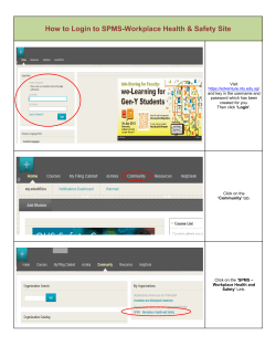
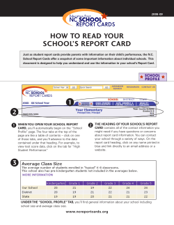
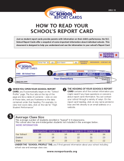
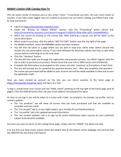
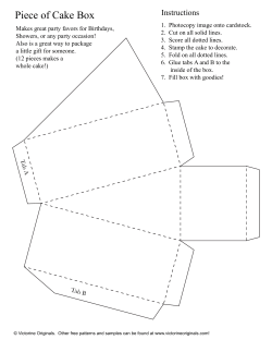


© Copyright 2026