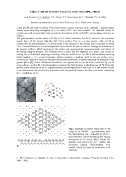
Home
Search
Collections
Journals
About
Contact us
My IOPscience
Reverse Monte Carlo study of spherical sample under non-periodic boundary conditions: the
structure of Ru nanoparticles based on x-ray diffraction data
This content has been downloaded from IOPscience. Please scroll down to see the full text.
2013 J. Phys.: Condens. Matter 25 454211
(http://iopscience.iop.org/0953-8984/25/45/454211)
View the table of contents for this issue, or go to the journal homepage for more
Download details:
IP Address: 141.209.165.173
This content was downloaded on 15/11/2013 at 13:38
Please note that terms and conditions apply.
IOP PUBLISHING
JOURNAL OF PHYSICS: CONDENSED MATTER
J. Phys.: Condens. Matter 25 (2013) 454211 (9pp)
doi:10.1088/0953-8984/25/45/454211
Reverse Monte Carlo study of spherical
sample under non-periodic boundary
conditions: the structure of Ru
nanoparticles based on x-ray diffraction
data
Orsolya Gereben1 and Valeri Petkov2
1
Institute for Solid State Physics and Optics, Wigner Research Centre for Physics, Hungarian Academy
of Sciences, PO Box 49, H-1525 Budapest, Hungary
2
Department of Physics, 203 Dow Science, Central Michigan University, Mt. Pleasant, MI 48859, USA
E-mail: [email protected]
Received 20 November 2012, in final form 11 March 2013
Published 18 October 2013
Online at stacks.iop.org/JPhysCM/25/454211
Abstract
A new method to fit experimental diffraction data with non-periodic structure models for
spherical particles was implemented in the reverse Monte Carlo simulation code. The method
was tested on x-ray diffraction data for ruthenium (Ru) nanoparticles approximately 5.6 nm in
diameter. It was found that the atomic ordering in the ruthenium nanoparticles is quite
distorted, barely resembling the hexagonal structure of bulk Ru. The average coordination
number for the bulk decreased from 12 to 11.25. A similar lack of structural order has been
observed with other nanoparticles (e.g. Petkov et al 2008 J. Phys. Chem. C 112 8907–11)
indicating that atomic disorder is a widespread feature of nanoparticles less than 10 nm in
diameter.
(Some figures may appear in colour only in the online journal)
1. Introduction
structural fluctuations. This renders the atomic ordering in
NPs essentially non-homogeneous, with a higher degree of
order in the NPs’ interior and a smaller degree of order at their
surface.
Traditionally the atomic-scale structure of materials
is obtained through diffraction-based techniques [9–11].
Combining diffraction data with reverse Monte Carlo
simulations (RMC) [12, 13] has turned out to be very useful in
structure studies of substantially disordered materials such as
amorphous semiconductors [14], glasses [15] and liquids [16].
Being finite, i.e. essentially non-periodic, and structurally
not quite homogeneous, the atomic-scale structure of NPs
poses a serious problem, known as the nanostructure problem [17]. The problem has been tackled by several techniques
with different amounts of success. For example, traditional
transmission electron microscopy (TEM) can provide information about the NPs’ size and morphology [18, 19].
With current technology moving fast into smaller dimensions,
nanoparticles (NPs) are produced at an increased rate
and explored for various applications [1–6]. The unique
functionality of NPs is due to finite size effects which
considerably modify their atomic-scale structure and, hence,
properties. Also, NPs have a large surface to volume ratio and
can interact with their environment, which is very beneficial
for biomedical [7] and catalytic applications [8]. Since the
atomic-scale structure predetermines the material’s properties
to a great extent, a big effort is underway to develop scientific
tools for determining the atomic ordering in NPs. The task is
not trivial since, contrary to the case of bulk crystals, atoms
in NPs do not sit on the vertices of periodic lattices [9].
Furthermore, atoms at the surface of NPs are less constrained
than those in the NPs’ core and so prone to larger scale
0953-8984/13/454211+09$33.00
1
c 2013 IOP Publishing Ltd Printed in the UK & the USA
J. Phys.: Condens. Matter 25 (2013) 454211
O Gereben and V Petkov
Yet TEM images are a projection down an axis and so not
so sensitive to the atomic ordering inside NPs, although a
combination of aberration-corrected scanning transmission
electron microscopy, statistical parameter estimation theory
and discrete tomography resulted in a 3D reconstruction
of the structure of a silver nanoparticle embedded in
an aluminum matrix [20]. Extended x-ray absorption fine
structure (EXAFS) is also very useful but yields information
˚ only.
about the atomic ordering extending out to 5–6 A
Thus, for example, an EXAFS experiment would hardly
distinguish between a hexagonal (hcp) and a face centered
cubic (fcc) ordering of atoms since both show first and second
coordination spheres of twelve and six atoms, respectively.
Among other techniques, total scattering experiments
coupled with Fourier-transform, atomic radial distribution
function (rdf), also called pair distribution function (PDF)
analysis, and computer simulations are becoming more widely
used in nanostructure studies [21, 22]. Depending on the
degree of atomic ordering in NPs, different simulation
techniques are employed to fit the experimental PDF data.
When NPs show considerable atomic order, crystalline
lattice-based models are employed that perform a least-square
fit between model calculated and experimental PDF data [23]
in a manner similar to the Rietveld refinement of powder
diffraction data. When the degree of atomic ordering in
NPs is low, simulated annealing [24] and reverse Monte
Carlo (RMC) [12, 25] do a better job. In the latter
type of modeling structural constraints imposed on atomic
coordination numbers, bond angles soon turn out to be very
useful for improving the simulations’ convergence and the
reliability of the produced structure models [26, 27]. Last
but not least, the good capabilities of the Debye function
approach in structure studies of NPs have to be acknowledged
as well [28]. Several comprehensive reviews on the various
modeling techniques applied in nanostructure studies are
available [29].
A particular feature of all the modeling techniques
mentioned above is that they apply periodic boundary
conditions on the model NP structures which, among other
things, makes the positions of atoms in NPs very strongly
correlated with each other. Real NPs are, however, finite and
have an open surface where the periodicity of the atomic
ordering is ultimately broken. If the rdf of a spherical sample
put inside a simulation box is calculated, then the rdf would
curve downward with increasing distance instead of tending
to one. In an attempt to take into account the finite size of
NPs, correction factors have been developed to modify the
computed radial distribution function [30]. Such correction
factors are useful but still work under the assumption of
infinite periodicity of the atomic ordering in NPs and so just
circumvent and do not solve the nanostructure problem.
We undertook the task to develop a version of the RMC
code, which will explicitly take into account the finite size
and broken periodicity of NPs. Here we describe the approach
we developed in some detail and the results of its testing
˚ in radius. The
on Ru particles that are approximately 28 A
new methodology was included in the simulation package
RMC POT [31, 32]. Note that production of Ru nanoparticles
is being attempted by various synthetic routes using different
substrates such as graphene [33], glassy carbon [34], a
metal–organic frame [35], an acetate/polyol-base [36] or
in aqueous solution [37], and are vigorously explored for
catalytic applications [36].
2. Methodology details
2.1. Derivation of a volume element for non-periodic
boundary conditions
By definition the rdf, g(r) = ρ(r)/ρo , where ρ(r) is the
average local and ρo the average atomic number density,
oscillates about one at large r values. (Usually ρ(r) is
only called the local number density, but now it has to be
distinguished from the local density around one particular
atom, so that is why it will be referred to as the average
local number density.) To ensure that the model g(r) computed
under non-periodic boundary conditions behaves in this way,
the derivation of the average local density ρ(r) had to be
modified.
Usually the partial average local density at distance r
from an atom of type b with respect to a central atom of type a
is calculated from an average partial histogram, n¯ ab (r). In the
case of r < L, where L is half of the simulation box length,
the following definition can be applied (1):
ρ¯ab (r) =
n¯ ab (r)
n¯ ab (r)
=
1V(r)
4/3π(ru3 − rl3 )
(1)
n¯ ab (r) =
Na
1 X
nm (r)
Na m=1 ab
(2)
where ru , rl are the upper and lower boundaries of the
histogram bin, r is the position of that bin’s center, Na is the
total number of atoms of type a and nm
ab (r) is the local partial
histogram of the mth atom of type a for neighbors of type b.
Here it is assumed that for every central atom of type a the
volume of the ith histogram bin, 1V(r), depends only on the
distance r from the central atom, and not on the position of
the central atom inside the simulation cell. This is so because,
under periodic boundary conditions, the cell is surrounded
with its mirror images.
From the average local density, the rdf, g(r), can be
calculated as follows:
gab (r) =
ρ¯ab (r)V
ρ¯ab (r)
=
ρb
Nb
(3)
where Nb is the total number of atoms of type b and V is the
simulation box volume.
Our model system under non-periodic boundary conditions will consist of a spherical sample placed into a cubic
simulation box. It will represent a system with spherical
particles with a known size, and narrow size distribution.
It will only account for the intra-particle correlations, but
as most of the inter-particle correlations are on a larger
distance scale the corresponding scattering would only appear
in the small angle scattering region, and would not affect the
simulation result.
2
J. Phys.: Condens. Matter 25 (2013) 454211
O Gereben and V Petkov
Figure 1. (a) Showing volume elements depending on the central atom’s position found inside the light blue zone (left side of figure: closer
to the center of the sample, right side of figure: close to the surface of the sample) and the size of the histogram bin, a smaller one depicted
as r1 (upper part of figure) and a larger one depicted as r2 (lower part of figure). Protruding volume elements of a histogram bin that is
outside sphere A with radius R0 are shown in red. (b) The protruding part of a volume element (red) that should be subtracted from the
spherical shells B and C. The volume element that is used in the normalization of the histogram is shown in green. The central atom is
located on the blue ring.
complete spherical shells (see the concentric circles with
outer radius r1 on the upper left part of figure 1(a)), while
others—fractions of spherical shells (shown in green in
figure 1(b)) are obtained subtracting the protruding volume
elements (shown in red in figure 1(b)) from the whole
spherical shell.
First we will calculate the protruding volume element
that is shown in red in figure 1(b). The radius of the smaller
and larger spheres C and B are related as rB,j = rC,j + 1r =
(j + 1)1r, where 1r is the size of the histogram bin. The
calculation can be divided into two steps, first calculating the
protruding part of sphere B from sphere A, Vout B (shown
in yellow in figure 2(a)) and then calculating the protruding
part of sphere C from sphere A, Vout C (shown in orange
figure 2(b)).
Note, the protruding volume depends on the radii of both
spheres B and C, and the positions of their origins. For the
sake of simplicity the origins are positioned at the middle of
each central histogram bin during the derivation leading to
only two independent variables for Vout B , Vout C .
The volume of the spherical cap cut off from sphere A is
denoted by VA yB (j, k) in figure 2(a). It can be computed as
follows:
In the case of non-periodic boundary conditions, the
volume of the histogram bin may not be the same for the same
atomic neighbor distances. Rather it will depend on r and the
position of the central atom in the simulation box, that is the
distance d of the central atom from the origin (see figure 1(a)).
As can be seen in the figure, for some central atoms this
volume element protrudes from the spherical surface of the
sample being modeled. As a result, the actual number of
neighbors for such atoms will be smaller than under periodic
boundary conditions.
So instead of first averaging the histogram bins to obtain
the average atom counts n¯ ab (r), an individual local number
density has to be calculated from any local histogram bin
using the respective volume element for each central atom.
Only then may the individual local number densities be
averaged out to obtain the average number density. From it
the rdf can be calculated using equation (3).
Whether a correction for the volume element is necessary
depends on the position of the central atom and the size of the
histogram bin (figure 1). In particular, the larger the volume
element, the more likely it will protrude from the model
spherical shell/surface, as shown in figure 1(a). On the left
side of figure 1(a) the central atom is positioned inside the
blue ring closer to the center of the sample and on the right
side very close to the surface of the sample. The upper part of
these figures shows histogram bins with a smaller radius r1 ,
while the lower part shows a larger histogram bin with radius
r2 . For the same central atom position the volume element
of the histogram bin is inside the sample for the smaller, r1
histogram bin (upper left part of figure), while protruding
from the sample (shown in red) for the larger histogram bin
with radius r2 (lower left part of figure 1(a)). The right side
of the figure is showing histogram bins with different origin
protruding from the sample to a different extent.
When the volume elements of each central atom are
calculated, it may happen that some of those elements are
VA yB (j, k) =
π 2
x (3R0 − xB )
3 B
(4)
where xB = mB + z − rB,j is the height of the cap. The volume
of the spherical cap cut off from sphere B, VB yB (j, k) (see
figure 2(b)) can be calculated in a similar manner, i.e.
VB yB (j, k) =
π 2
m (3rB − mB ).
3 B
(5)
As shown in figures 2(a) and (b), z = R0 − (k + 0.5)1r.
To determine xB , the following two equations using the rules
of a right angle triangle can be written (6). Note, from these
3
J. Phys.: Condens. Matter 25 (2013) 454211
O Gereben and V Petkov
Figure 2. (a) Sketch of the volume elements of sphere B protruding from sphere A. The spherical caps of sphere A and B are cut off by the
same plane and have a circular base with a radius of yB . The volume of the spherical cap A (cut off from sphere A) is VA yB (j, k) (see (a), in
gray), the volume of the spherical cap B cut off from sphere B is VB yB (j, k) (see the cumulated volume of gray and yellow in (a)). (b) The
volume element of sphere C protruding from sphere A is shown. The spherical caps of sphere A and C cut off by the same plane have a
circular base with yC radius. The volume of the spherical cap A (cut off from sphere A) is VA yC (j, k) (see (a), pink) while the volume of the
spherical cap C cut off from sphere C is VC yC (j, k) (shown in (b) in pink and orange).
If only sphere B is protruding from sphere A, which
takes place if 0 < rB,j − z < 1r, the following relationship
applies: Vout (j, k) = Vout B (j, k), where Vin (j, k) is calculated
according equation (10). If neither of spheres B and C are
protruding from sphere A no volume element correction is
necessary.
For each atom, a central bin index, k (see figure 2(b)),
is assigned indicating which bin the atom belongs to. These
bin indices are calculated at the beginning of the RMC
simulation, and then updated when an atom is moved to
another bin. The volume element Vin (j, k) will be the same
for all the atoms belonging to the same central bin (with their
distance, d from the origin between k1r and (k + 1)1r),
as this is computationally more efficient than calculating
and storing a series of individual volume elements for each
atom. When 1r is small enough, this approximation will have
little impact on the simulation results. Finally, in the case of
non-periodic boundary conditions the average local density
can be equation (11):
equations both xB and mB can be determined.
I. R20 = (R0 − xB )2 + y2B
2
II. rB,j
= (z − xB )2 + y2B
2
z2 − rB,j
xB =
.
2z − 2R0
(6)
As a result the volume designated in yellow in figure 2
can be calculated as follows:
Vout B (j, k) = VB yB (j, k) − VA yB (j, k).
(7)
Following the same reasoning scheme we can write that
xC = mC + z − rC,j0 where xC and mC are determined from
equation (8).
I. R20 = (R0 − xC )2 + y2C
2
II. rC,j
= (z − xC )2 + y2C
2
z2 − rC,j
.
xC =
2z − 2R0
(8)
ρ¯ab (r) =
The spherical caps with a circular base and a radius yC
cut off from spheres A and C can be calculated as follows:
π 2
VA yC (j, k) = xC
(3R0 − xC )
3
π 2
VC yC (j, k) = mC (3rC − mC ).
3
j1r ≤ r < (j + 1)1r
k1r ≤ dm < (k + 1)1r.
(11)
It is worth noting that while the system modeled is
spherical in shape, its surface need not be smooth but may
have edges and steps as it frequently occurs with real NPs.
During the simulation atoms inside the spherical sample
are moved around, and only those moves that keep the
atoms within the model sphere are considered for acceptance
according to the usual RMC acceptance scheme [12].
In figure 3 the correctly normalized rdf for a finite size,
non-periodic, randomly distributed spherical model system is
compared to an rdf of the same spherical sample situated in a
cubic simulation box subject to periodic boundary conditions.
The latter rdf shows unphysical sloping across the whole
range of r values while the g(r) computed via equations (3)
and (11) oscillates about one as it should according to its
definition.
(9)
The volume element of sphere C protruding from sphere
A (shown in orange in figure 2(b)) is defined as Vout C (j, k) =
VC yC (j, k) − VA yC (j, k). Based on this definition, the
protruding spherical shell (shown in red in figure 1(b)) can be
computed as Vout (j, k) = Vout B (j, k) − Vout C (j, k). Note all
these relationships are valid when both spheres B and C are
protruding from sphere A, which takes place if rB,j − z > 1r.
Given this, the volume element remaining inside sphere A is
Vin (j, k) = 1Vj − Vout (j, k)
3
3
= 43 π(rB,j
− rC,j
) − Vout (j, k).
Na
nm
1 m
1 X
ab (r)
=
ρ (r)
Na m=1 1Vin (j, k)
Na ab
(10)
4
J. Phys.: Condens. Matter 25 (2013) 454211
O Gereben and V Petkov
3.2. TEM characterization
Transmission electron microscopy (TEM) was performed
on a FEI Tecnai 20 electron microscope at an acceleration
voltage of 200 kV with a LaB6 filament. A small amount
of the sample was diluted with ethanol, dispersed and dried
over a carbon-coated Cu grid. Particle size distribution was
calculated by measuring more than 150 particles. The NPs we
˚
studied had an average diameter of 56(±5) A.
3.3. X-ray diffraction experiments
XRD data was collected at the beamline 11-ID-C at the
Advanced Photon Source, Argonne National Laboratory,
˚ The sample was in
using x-rays of wavelength 0.1078 A.
a glass capillary. An image plate detector was used. The
XRD data were corrected for background and Compton
scattering, normalized into absolute electron units using the
RAD software [39].
Note that the high-energy XRD pattern and its Fourier
counterpart, the atomic rdf, reflect assembly averaged
structural features of all Ru nanoparticles sampled by
the x-ray beam in the same way that traditional powder
XRD represents an assembly average of all polycrystallites
sampled by the x-ray beam in those experiments. Comparing
a particle’s assembly averaged structure features to a
particle’s assembly averaged properties (e.g., catalytic) puts
the structure–property relationship exploration on the same
footing.
Figure 3. Behavior of the rdfs for a spherical randomly distributed
sample calculated under periodic (blue) and non-periodic (red)
boundary conditions. Note the unphysical sloping of the rdf
computed under periodic boundary conditions.
2.2. Average coordination constraints
The calculation of the average coordination constraint under
non-periodic boundary conditions has to be modified as well,
in particular for atoms close to the surface of the spherical
sample being modeled. Note those atoms will, on average,
have a smaller number of neighbors than atoms in the sample’s
interior. Accordingly, the average coordination number is
calculated only for atoms which are inside a sphere of radius
R0 − d, where d = (dmax − dmin )/2 and dmin , dmax are the
limiting range values of the atomic coordination sphere.
3.4. RMC simulations
3. Experimental and simulation details
The RMC simulation was performed on a 6841 Ru
atoms-containing spherical configuration closely resembling
˚ in diameter. The number
a spherical NP approximately 56 A
˚ −3 corresponding to 12.45 g cm−3
density of 0.074 39 A
was used. A hexagonal closely packed (hcp) spherical
configuration cut out from a crystalline lattice of Ru was used
as a starting point of the RMC simulations. The simulations
were guided by the experimental structure factor and were
stopped when the RMC computed and experimental data
agreed very well over the whole range of wavevectors reached
˚ −1 . The
by the present experiments, i.e. from about 2 to 30 A
simulation was carried out with the help of a new version
of RMC POT software [31, 32] furnished for the case of
non-periodic boundary conditions. Computations were done
R
R
on an Intel
Xeon
CPU E5345 2.33 GHz 2*quad core
processor computer, using 4 threads. An average coordination
˚
constraint enforcing 12 first neighbors between 2.1 and 3.5 A
was applied to take into account the close-packed nature of
the Ru metal structure.
3.1. Preparation of Ru nanoparticles
Polyvinylpyrrolidone (PVP, Mn = 10 000 g mol−1 , Sigma
Aldrich) stabilized Ru nanoparticles with a diameter of
˚ were synthesized as part of a series of particles with
∼56 A
different sizes [38] by using 1,4-butanediol or H2 as the
reducing agent. In a typical synthesis PVP/Ru molar ratio
of 20 was applied. 30 mg of ruthenium(III) acetylacetonate
(Aldrich) and 0.17 g of PVP were dissolved in 2 cm3
of tetrahydrofuran (THF, Sigma Aldrich) and 3 cm3 of
1,4-butanediol (Sigma Aldrich). This mixture was added to
27 cm3 of 1,4-butanediol, which was preheated at 225 ◦ C,
followed by refluxing in a N2 atmosphere for 2 h. The
resulting black mixture was thoroughly washed with acetone
and diethyl ether. After collecting the Ru nanoparticles by
centrifugation, they were redispersed in 1.5 cm3 distilled
water. In cases where reduction was carried out in hydrogen,
first 40 mg of RuCl3 ·xH2 O (Alfa Aesar) and 0.22 g of PVP
were dissolved in 1 cm3 of distilled water in a 10 cm3
autoclave. The autoclave was then pressurized with 20 bar
H2 followed by heating to 150 ◦ C for 2 h under vigorous
stirring. The resultant black mixture was washed, collected by
centrifugation, and redispersed in 3 cm3 distilled water.
4. Results and discussion
The RMC simulated and experimental XRD structure
factors and their differences are shown in figure 4(a). The
experimental structure factor shows broad diffraction features
5
J. Phys.: Condens. Matter 25 (2013) 454211
O Gereben and V Petkov
˚ radius Ru
Figure 4. (a) The experimental (symbol +), the RMC-fitted (line) structure factors and their difference (symbol ×) of 28 A
particles. (b) The ‘experimental’ G(r) (symbol +) and the fit produced by the PDFgui program (line) assuming Ru hcp lattice periodicity.
˚ in radius
Figure 5. (a) The rdf for the RMC simulated model. (b) Low-r parts of the rdfs for the RMC simulated model of Ru particles 28 A
(line in blue) and for the crystalline hexagonal close packed (hcp) lattice of bulk Ru (line in red).
that are usually seen with heavily disordered materials. For
comparison a fit to the ‘experimental’ PDF G(r) calculated
by direct Fourier transformation of the experimental structure
factor performed by the PDFgui [40] program assuming the
lattice periodicity of bulk Ru hcp is shown in figure 4(b). The
relationship between G(r) and g(r) is G(r) = 4π rρ0 (g(r)−1).
As is visible, the major features are recreated, but there is
a substantial difference in the peak heights showing that the
periodic model cannot sufficiently reproduce the structure.
The simulated rdf g(r) is shown in figure 5(a). It decays
˚ indicating that the Ru NPs
to one at distances of about 15 A,
studied by us exhibit only short to medium but definitely not
long-range order.
The average coordination number in the interior of the NP
model decreased a bit from 12 to 11.25 due to the presence
of strong local disorder manifested by the broad character of
the first rdf peak. The coordination numbers in the bulk are
spreading from 7 to 17, 19% of the atoms having still 12 and
18% having 13 neighbors. The coordination numbers of the
atoms at the NPs’ surface were considerably smaller than 12
due to free surface effects.
The rdfs of the hexagonal close packed lattice of bulk Ru
˚ radius Ru particles are
and the RMC generated rdf for 28 A
compared in figure 5(b). As can be seen from the figure, the
first rdf peak for the RMC generated model is considerably
broadened when compared to the same peak in the rdf for bulk
Ru. Note the first rdf peak for bulk Ru reflects the presence of
12 first atomic neighbors, 6 from the plane (denoted as A; see
figure 6) where the atom chosen for the central one denoted
as O resides, and 3–3 more (labeled as number 1, displayed
in dark green) from the planes above and below this atom.
This observation indicates that the first coordination sphere in
Ru NPs is considerably distorted when compared to the first
coordination sphere of bulk Ru. The position of the second
coordination sphere (containing six second neighbors labeled
as number 2, light green in planes B) in Ru NPs has slightly
moved to longer interatomic distances. Furthermore, the third
rdf peak (coming from the atoms labeled as O0 in the next
planes A above and below the atom in the origin) of the hcp
lattice appears completely smeared out in the model rdf for
Ru NPs. The fourth (planes B third neighbors, and same plane
as origin second neighbors, neither shown in the picture) and
fifth peaks (planes A above and below, atoms labeled as 1) of
the hpc merged together for the NP, and further identification
of the peaks is not possible.
A closer examination of the RMC generated configuration shown in figure 7 reveals that the hexagonally closed
packed atomic planes of bulk Ru are still recognizable in
˚ radius particles. This observation
the model for the 28 A
indicates that Ru NPs studied here share some of the structural
˚
features of their bulk counterpart. Next, we explored a 2.273 A
thick slice containing the central plane of the spherical
sample cut out from the RMC generated model. Two different
values for the spatial extent of the first atomic coordination
˚ (figure 7(a)) and 3.5 A
˚ (figure 7(b)), were
sphere, 2.8 A
˚ is
used for the coordination number coloring. Note 2.8 A
the radius of the first atomic coordination sphere in bulk
Ru where each atom has 6 very first neighbors forming a
flat planar atomic configuration (see figure 6). On the other
˚ is the first minimum in the RMC generated rdf
hand, 3.5 A
which can be considered as a radius of the first coordination
sphere for the Ru NPs under investigation. As can be seen
in figure 7(a), only a few atoms have six first neighbors
˚ was applied as a cut off
sitting on a flat plane. When 3.5 A
6
J. Phys.: Condens. Matter 25 (2013) 454211
O Gereben and V Petkov
consistent with the substantial broadening of the first rdf peak
indicating substantial disorder in the positions of the near
atomic neighbors in Ru NPs.
To explore the three-dimensional structure of Ru NPs in
˚ was cut
more detail, a spherical cluster with a radius of 5.1 A
off from the very center of the RMC produced configuration,
and displayed from two different points of view. The radius
˚ was chosen since this real space distance entails the
of 5.1 A
first five coordination spheres in bulk Ru. Again, a cut off
˚ was applied as a radius of the first atomic
distance of 3.5 A
coordination sphere. In figure 8(a) the cluster is presented
along close packed atomic planes similar to the hcp planes
occurring in bulk Ru. In figure 8(b) the same cluster is viewed
from the direction of the c crystallographic axis, perpendicular
to the planes. The results presented in figure 8(a) clearly show
that (i) close packed though somewhat buckled atomic planes
do exist in Ru NPs and (ii), as in bulk Ru, the planes are
stacked up together. The atoms within these planes, however,
are not arranged on the vertices of regular hexagons but are
scattered in various in-plane directions (see figure 8(b)).
To check if the entire Ru NP model shares the features
of its core discussed above, two orientational rdfs were
computed in two orthogonal directions. One of the directions
is along the c crystallographic axis in the Ru NP model,
the other—perpendicular to that (labeled later as a–a).
The orientational rdfs, gc (r) and ga–a (r) were calculated
similarly to g(r) using appropriate normalizations due to
the different sample volumes, and only those atom pairs
were included in the calculation where the difference of
the coordinate components of the atom pairs (in the case
of gc (r) perpendicular to the c-axis, in the case of ga–a (r)
˚
perpendicular to the a–a plane) were smaller than 0.1 A.
The normalized auto-correlation function was calculated
Figure 6. Two unit cells of the hcp structure of bulk Ru stacked on
top of each other. The parameters of the hcp lattice are
˚ c = 4.28 A.
˚
a = 2.7 A,
radius of the first coordination sphere, the number of atoms
having 6 first neighbors forming a planar-type configuration
increased considerably (see figure 7(b)). These results are
˚
Figure 7. Slice containing the largest plane incorporating the a–a crystallographic axis of the spherical RMC generated model for 28 A
˚ was used for the upper limit of the atomic first coordination sphere. (b) A cut off value of
radius Ru particles. (a) A cut off value of 2.8 A
˚ was applied. The following coloring scheme was applied to differentiate between atoms with a different number of first atomic
3.5 A
neighbors sitting on a plane: 0 neighbors: white; 1 neighbor: turquoise; 2 neighbors: beige; 3 neighbors: green; 4 neighbors: gray; 5
neighbors: red; 6 neighbors: brown; 7 neighbors: purple.
7
J. Phys.: Condens. Matter 25 (2013) 454211
O Gereben and V Petkov
˚ cut out from the center of the RMC produced atomic configuration. The cluster is
Figure 8. Spherical cluster with a radius of 5.1 A
presented in two different orientations as described in the text. The coloring of the atoms reflects the atomic planes they belong to.
applying periodic boundary conditions was developed. When
applied the method allows the testing and refining of structure
models based directly on the diffraction data of spherical
samples like nanoparticles with a free surface and, when
present, inhomogeneities in the atomic ordering.
The method would perform best with diffraction data
for particles with known size, a narrow size distribution
and spherical shape. Note the method does not take into
account possible inter-particle correlations. This is, however,
not a severe limitation considering the fact that inter-particle
correlations are typically long ranged. Such correlations are
best revealed by small angle scattering, which is usually not
included in the XRD data aimed at atomic rdf analysis.
˚
The method was tested on Ru NPs approximately 28 A
in radius. Analysis of the resultant structure model showed
that the NPs possess some of the structural features of bulk
Ru, in particular the presence of close packed atomic layers
that are stacked up together. The overall atomic-scale structure
of the NPs, however, is quite distorted at both short and
long-range atomic distance with the degree of structural
disorder exhibiting a strong orientational dependence. This
will definitely impact on the catalytic properties of the NPs
which will be discussed elsewhere.
Figure 9. Auto-correlation functions for the orientational rdfs in Ru
NPs calculated along the buckled atomic planes, (designated as a–a
plane, line in red) and perpendicular to them (designated as c axis,
line in blue).
according to the formula:
C(rj ) =
!
!
Nj
N0
1 X
1 X
g(ri )g(ri+0 ) (12)
g(ri )g(ri+j )
Nj i
N0 i
where ri , rj are the ith and jth distance bin, Nj = Nmax −
j. The auto-correlation functions of these rdfs are shown
in figure 9. Results in the figure indicate much stronger
interatomic correlations in a direction perpendicular to the
atomic planes (along the c-axis). Correlation lengths were
estimated from the asymptotic part of the auto-correlation
functions, C(r), using the relation: ln(C(r)) ∼ −(r/ξ ), where
r is the radial distance and ξ is the so-called correlation
length. The correlation lengths turned out to be about ξa–a =
˚ along the planes and ξc = 31.4±0.1 in a direction
18.9±0.1 A
perpendicular to the planes, clearly indicating that the degree
˚ radius is
of structural disorder in the studied RuNP of 28 A
highly inhomogeneous.
Acknowledgment
The authors are thankful for financial support from DOE-BES
via Grant DE-SC0006877.
References
[1] Yang S, Damiano M G, Zhang H, Tripathy S, Luthi A J,
Rink J S, Ugolkov A V, Singh A T K, Dave S S,
Gordon L I and Thaxton C S 2013 Proc. Natl Acad. Sci.
110 2511
[2] Jeong Y-H, Yoon H-J and Jang W-D 2012 Polym. J. 44 512
[3] Philip J, Kumar T J, Kalyanasundaram P and Raj B 2003
Meas. Sci. Technol. 14 1289
[4] Mornet S, Vasseur S, Grasset F, Verveka P, Goglio G,
Demourgues A, Portier J, Pollert E and Duguet E 2006
Prog. Solid State Chem. 34 237
[5] Hyeon T 2003 Chem. Commun. 927
5. Conclusion
A new method for reverse Monte Carlo-type simulations
of the atomic-scale structure of spherical particles without
8
J. Phys.: Condens. Matter 25 (2013) 454211
O Gereben and V Petkov
[23] Proffen Th and Billinge S J L 1999 J. Appl. Crystallogr.
32 572
[24] Toby B H, Egami T, Jorgensen J D and
Subramanian M A 1990 Phys. Rev. Lett. 64 2414
[25] Tucker M G, Dove M T and Keen D A 2001 J. Appl.
Crystallogr. 34 630
[26] Wells S A, Dove M T and Tucker M G 2002 J. Phys.:
Condens. Matter 14 4567
[27] Sartbaeva A, Wells S A, Thorpe M F, Boˇzin E S and
Billinge S J L 2007 Phys. Rev. Lett. 99 155503
[28] Cervellino A, Giannini C and Guagliardi A 2006 J. Comput.
Chem. 27 995
[29] Billinge S J L 2008 J. Solid State Chem. 181 1695
Proffen T 2006 Rev. Mineral. Geochem. 63 255
[30] Kodama K, Iikubo S, Taguchi T and Shamoto S 2006 Acta
Crystallogr. A 62 444–53
[31] Gereben O and Pusztai L 2012 J. Comput. Chem. 33 228
[32] RMC POT Website: www.szfki.hu/∼nphys/rmc++/opening.
html
[33] Liu X, Yao K X, Meng C and Han Y 2012 Dalton Trans.
41 1289–96
[34] Rahman G, Yeon Lim J, Jung K-D and Joo O-S 2011 Int. J.
Electrochem. Sci. 6 2789–97
[35] Zhao Y, Zhang J, Song J, Li J, Liu J, Wu T, Zhang P and
Han B 2011 Green Chem. 13 2078–82
[36] Bedford N, Dablemont C, Viau G, Chupas P and
Petkov V 2007 J. Phys. Chem. C 111 18214
[37] Lu F, Liu J and Xu J 2008 Mater. Chem. Phys. 108 369–74
[38] Hensen E J M 2012 unpublished
[39] Petkov V 1989 J. Appl. Crystallogr. 22 387
[40] Farrow C L, Juhas P, Liu J W, Bryndin D, Boˇzin E S, Bloch J,
Proffen Th and Billinge S J L 2007 J. Phys.: Condens.
Matter 19 335219
[6] Elliott D W and Zhang W-X 2001 Environ. Sci. Technol.
35 4922
[7] Gupta A K and Gupta M 2005 Biomaterials 26 3995
[8] Lu A-H, Schmidt W, Matoussevitch N, B¨onnemann H,
Spliethoff B, Tesche B, Bill E, Kiefer W and Sch¨uth F 2004
Angew. Chem. Int. Edn 43 4303
[9] Petkov V, Bedford N, Knecht M R, Weir M G, Crooks R M,
Tang W, Henkelman G and Frenkel A 2008 J. Phys. Chem.
C 112 8907–11
[10] Petkov V, Moreels I, Hens Z and Ren Y 2010 Phys. Rev. B
81 241304
[11] Whitfield P and Mitchell L 2004 Int. J. Nanosci. 3 757
[12] McGreevy R L and Pusztai L 1988 Mol. Simul. 1 359
[13] McGreevy R L 1995 Nucl. Instrum. Methods A 354 1
[14] Gereben O and Pusztai L 1994 Phys. Rev. B 50 14136
Fukunaga T, Itoh K, Otomo T, Mori K, Sugiyama M, Kato H,
Hasagawa M, Hirata A, Hirotsu Y and Aoki K 2006
Physica B 385 259
[15] Gereben O and Pusztai L 1994 Mater. Sci. Eng.
A179–A180 433
[16] Mile V, Gereben O, Kohara S and Pusztai L 2010 J. Mol. Liq.
157 36
[17] Billinge S J L and Levin I 2007 Science 316 561
[18] Rutledge R D, Morris H, Wellons M S, Zheng G, Shen J,
Bentley J, Wittig J E and Lukehart M 2006 J. Am. Chem.
Soc. 128 14210
[19] Sun S, Anders S, Thomson T, Baglin J E E, Toney M F,
Hamann H F, Murray C B and Terris B D 2003 J. Phys.
Chem. 107 5419
[20] van Aert S, Batenburg K J, Rossell M D, Erni R and
van Tendeloo G 2011 Nature 470 374
[21] Egami T and Billinge S J L 2003 Underneath the Bragg
Peaks: Structural Analysis of Complex Materials
(Amsterdam: Elsevier)
[22] Billinge S J L and Kanatzidis M G 2004 Chem. Commun.
2004 749
9