
XMAS: an open MIDI and sample-based music system Computer Science Tripos Robinson College
Ben Davis XMAS: an open MIDI and sample-based music system Computer Science Tripos Robinson College May 9, 2004 Proforma Name: College: Project Title: Examination: Word Count: Originator: Supervisor: Ben Davis Robinson College XMAS: an open MIDI and sample-based music system Computer Science Tripos 2004 11302 Ben Davis Neil Johnson Original Aims of the Project To provide a good solution by which a composer can write and distribute music to be played by a machine, particularly as part of a downloadable computer game. .mid files depend heavily on the hardware or software available at the destination; .mp3, .ogg and similar files are too large in many cases; Amiga-based module files (e.g. .mod, .s3m, .xm and .it) are difficult to compose and the playback behaviour is not well defined. This project aimed to produce an open source system that would avoid all of these problems. Work Completed An XML-based structure that allows a .mid author to build his or her own instrument sounds using .wav files was designed. A software library for parsing the structure and rendering the music to a mono or stereo PCM sample stream was written. In particular this incorporated a real-time resampler with cubic interpolation and a MIDI player. The project is fairly mature and will soon be available at http://xmas.sf.net/. Special Difficulties None. i Declaration I, Ben Davis of Robinson College, being a candidate for Part II of the Computer Science Tripos, hereby declare that this dissertation and the work described in it are my own work, unaided except as may be specified below, and that the dissertation does not contain material that has already been used to any substantial extent for a comparable purpose. Signed Date ii Contents 1 Introduction 1.1 The Technology . . . . . . . . . . . . 1.1.1 MIDI . . . . . . . . . . . . . . 1.1.2 Samples and Streamed Audio 1.1.3 Amiga mod-based Files . . . . 1.2 The Problem . . . . . . . . . . . . . 1.3 The Solution . . . . . . . . . . . . . . . . . . . . . . . . . . . . . . . . . . . . . . . . . . . . . . . . . . . . . . . 2 Preparation 2.1 Requirements . . . . . . . . . . . . . . . . . . . . 2.2 Initial Analysis of Requirements . . . . . . . . . . 2.2.1 Using Industry Standards . . . . . . . . . 2.2.2 Compression and Kolmogorov Complexity 2.2.3 Structure and Tweaks . . . . . . . . . . . 2.2.4 Same Output Everywhere . . . . . . . . . 2.3 Project Layout . . . . . . . . . . . . . . . . . . . 2.4 Further Analysis . . . . . . . . . . . . . . . . . . 2.4.1 Real-Time Playback . . . . . . . . . . . . 2.4.2 Third-Party Players . . . . . . . . . . . . . 2.5 Choice of Programming Language . . . . . . . . . 2.6 Refining the File Structure . . . . . . . . . . . . . 2.7 Final Preparations . . . . . . . . . . . . . . . . . 2.7.1 Core Requirements . . . . . . . . . . . . . 2.7.2 Extensions . . . . . . . . . . . . . . . . . . 2.7.3 Work Plan and Timetable . . . . . . . . . 2.7.4 Libraries and Code Used . . . . . . . . . . 2.7.5 Documentation Used . . . . . . . . . . . . 2.7.6 Code Management and Back-ups . . . . . iii . . . . . . . . . . . . . . . . . . . . . . . . . . . . . . . . . . . . . . . . . . . . . . . . . . . . . . . . . . . . . . . . . . . . . . . . . . . . . . . . . . . . . . . . . . . . . . . . . . . . . . . . . . . . . . . . . . . . . . . . . . . . . . . . . . . . . . . . . . . . . . . . . . . . . . . . . . . . . . . . . . . . . . . . . . . . . . . . . . . . . . . . . . . . . . . . . . . . . . . . . . . . . . 1 1 2 2 3 4 5 . . . . . . . . . . . . . . . . . . . 7 7 7 7 7 8 9 9 10 10 10 10 10 11 11 11 11 12 13 13 3 Implementation 3.1 Overview . . . . . . . . . . . . . . . . . . 3.1.1 Digital Signal Processing Modules 3.1.2 The State Tree . . . . . . . . . . 3.1.3 Generating the Music . . . . . . . 3.2 The XML . . . . . . . . . . . . . . . . . 3.3 Variables . . . . . . . . . . . . . . . . . . 3.4 Parameter Tweaks . . . . . . . . . . . . 3.5 The Modules . . . . . . . . . . . . . . . 3.5.1 Samples . . . . . . . . . . . . . . 3.5.2 Volume Envelopes . . . . . . . . . 3.5.3 Multiplexers . . . . . . . . . . . . 3.5.4 MIDI Mappings . . . . . . . . . . 3.5.5 Variable Compute Blocks . . . . . 3.6 The MIDI Playback Algorithm . . . . . 3.6.1 Overview . . . . . . . . . . . . . 3.6.2 State . . . . . . . . . . . . . . . . 3.6.3 Notes . . . . . . . . . . . . . . . 3.6.4 Algorithm . . . . . . . . . . . . . 3.6.5 Noteworthy Features . . . . . . . 4 Evaluation 4.1 Goals Achieved . . . . . . . . . . . 4.2 Evolution of the Plan . . . . . . . . 4.2.1 Generalisation . . . . . . . . 4.2.2 Filtering Whole Channels or 4.2.3 Reference Counting . . . . . 4.3 Milestones . . . . . . . . . . . . . . 4.4 Testing . . . . . . . . . . . . . . . . 4.4.1 General . . . . . . . . . . . 4.4.2 The Resampler . . . . . . . 4.5 Profiling . . . . . . . . . . . . . . . 4.6 Comments . . . . . . . . . . . . . . 4.6.1 Samples . . . . . . . . . . . 4.6.2 Volume Envelopes . . . . . . 4.6.3 MIDI Playback . . . . . . . 4.6.4 Flexibility . . . . . . . . . . 4.7 Problems Encountered . . . . . . . 4.7.1 STL Containers . . . . . . . iv . . . . . . . . . . . . . . . . . . . . . . . . . . . . . . . Tracks . . . . . . . . . . . . . . . . . . . . . . . . . . . . . . . . . . . . . . . . . . . . . . . . . . . . . . . . . . . . . . . . . . . . . . . . . . . . . . . . . . . . . . . . . . . . . . . . . . . . . . . . . . . . . . . . . . . . . . . . . . . . . . . . . . . . . . . . . . . . . . . . . . . . . . . . . . . . . . . . . . . . . . . . . . . . . . . . . . . . . . . . . . . . . . . . . . . . . . . . . . . . . . . . . . . . . . . . . . . . . . . . . . . . . . . . . . . . . . . . . . . . . . . . . . . . . . . . . . . . . . . . . . . . . . . . . . . . . . . . . . . . . . . . . . . . . . . . . . . . . . . . . . . . . . . . . . . . . . . . . . . . . . . . . . . . . . . . . . . . . . . . . . . . . . . . . . . . . . . . . . . . . . . . . . . . . . . . . . . . . . . . . . . . . . . . . . . . . . . . . . . . . . . . . . . . . . . . . . . . . . . . . . . . . . . . . . . . . . . . . . . . . . . . . . . . . . . . . . . . . . . . . . . . . . . . . . . . . . . . . . . . . . . . . . . . . . . . . . . . . . . 15 15 15 16 16 17 17 19 20 20 22 24 25 25 25 25 26 27 28 28 . . . . . . . . . . . . . . . . . 31 31 32 32 32 33 33 34 34 34 34 38 38 38 39 39 39 39 4.7.2 4.7.3 XML Files . . . . . . . . . . . . . . . . . . . . . . . . . . . Code Size . . . . . . . . . . . . . . . . . . . . . . . . . . . 40 40 5 Conclusions 41 Bibliography 43 A The Cubic Interpolation Function 45 B Some Example XML B.1 volenv.xml . . . . B.2 compute.xml . . . B.3 clarinet.xmi . . . B.4 pizz.xmi . . . . . B.5 general.xmi . . . B.6 Example Music . . 47 47 48 48 49 50 50 . . . . . . . . . . . . . . . . . . . . . . . . . . . . . . . . . . . . . . . . . . . . . . . . . . . . . . . . . . . . . . . . . . . . . . . . . . . . . . . . . . . . . . . . . . . . . . . . . . . . . . . . . . . . . . . . . . . . . . . . . . . . . . . . . . . . . . . . . . . . . . . . . . . . . . . . . . . . C Demo CD Track Listing 52 D Project Proposal 54 v List of Figures 3.1 3.2 3.3 3.4 3.5 An example piece of music . . . . . A state tree, with variables . . . . . How variables are implemented . . The history buffer . . . . . . . . . . Two examples of volume envelopes . . . . . . . . . . . . . . . . . . . . . . . . . . . . . . . . . . . . . . . . . . . . . . . . . . . . . . . . . . . . . . . . . . . . . . . . . . . . . . . . . . . . . 15 18 19 21 22 4.1 4.2 4.3 4.4 How to filter a set of channels . . The visual resampler test. . . . . The three interpolation functions. Some profiling results . . . . . . . . . . . . . . . . . . . . . . . . . . . . . . . . . . . . . . . . . . . . . . . . . . . . . . . . . . . . . . . . . . . . . . . . . . . 33 35 36 37 vi . . . . Acknowledgements Many thanks are due to Neil Johnson, my Project Supervisor, for the guidance he offered right from inception up until the final deadline. Thanks also go to Dr Alan Mycroft, my Director of Studies, for his assistance with this dissertation. The Dissertation was written inside the skeleton structure provided by Dr Martin Richards’ How to write a dissertation in LATEX [8]. vii viii Chapter 1 Introduction Electronic music is an exciting field. Many people will insist that it is no substitute for conventional acoustic music, and they are right. Acoustic instruments— and human performance—are an enormous challenge to emulate. Electronic music is not a substitute: it is a complement. It is a whole new world, populated with many synthesisers and filters, each with its own distinctive character, and free of such constraints as the span of a pianist’s hand. Moreover, it can all be done in software inside any reasonably modern computer equipped with a sound card and speakers. I am a proficient pianist and have composed a great deal of professional quality music. This strong musical background enabled me to hear bugs in my project’s output and reason about sound quality. 1.1 The Technology The best known example of an electronic musical instrument is an electronic keyboard. This features a piano-like keyboard, a pair of speakers and a range of buttons, and is capable of producing many different instrument sounds, from approximations of acoustic instruments to sounds unlike anything heard in the acoustic or natural world. There are other types of electronic musical instrument too: MIDI controllers feature just the keyboard, while MIDI modules 1 feature just the synthesiser. These devices have to be connected together to function. Sequencers allow music to be recorded or programmed, and can then play it back if a synthesiser is connected. 1 The word ‘module’ has different meanings in different contexts. The intended meaning will always be clear in this dissertation. 1 2 1.1.1 CHAPTER 1. INTRODUCTION MIDI Enter the MIDI Specification [1]. It was created in 1983 by Sequential Circuits, Roland and several other major synthesiser manufacturers as a protocol to allow instruments to communicate with one another. There are 16 channels, numbered from 1 to 16; a device can respond to events on some channels and not others, or assign different instruments to different channels. Events such as the following can be encoded in a byte stream and sent between devices: 9c nn vv Note On 8c nn vv Note Off Cc pp Program Change Start note at pitch nn on channel c + 1 with velocity vv, a measure of how hard the key on the keyboard was hit. Stop note at pitch nn on channel c + 1. The velocity vv here is a measure of how quickly the key was lifted. Assign program pp to channel c + 1. A program is typically an instrument sound, but some devices use it for other purposes such as rhythm selection. The first byte is known as the status byte. There are many other commands, but the status byte is always in the range 80–FF, and data bytes are always in the range 00–7F. If the same command is used repeatedly, the status byte only need be specified once, and it becomes the running status. MIDI commands can also be saved with time stamps in a Standard MIDI File. Such a file has the extension .mid. XMAS uses the .mid file as a major component in a piece of music. General MIDI, an addition made to the standard in 1991, designates a standard set of instrument names for the 128 integers that can be used in a Program Change command. It further allows a single channel to be used for unpitched percussion (such as cymbal crashes), with standard percussive instrument names assigned to many of the 128 note values. On multi-part synthesisers, it is usual for Channel 10 to contain percussion. 1.1.2 Samples and Streamed Audio When we hear sounds, our ears are detecting longitudinal oscillations, or pressure waves, in the air. These waves cause our eardrums to vibrate. A microphone uses a diaphragm to detect the waves and convert them into a varying electric current. This current can be sampled at discrete intervals, a common rate being 44100 Hz, and stored in a .wav file. The individual samples—or sample points—usually 1.1. THE TECHNOLOGY 3 have 16-bit values. Many recordings have two channels, one for each speaker in a stereo set-up;2 here, the sample points are interleaved, and each left-right pair is called a sample frame. This system for encoding sound as a series of samples is called Pulse Code Modulation, or PCM . It is possible to store an arbitrary number of channels in a .wav file, but it is rare for more than two to be stored. A sample, in one sense of the overappropriated word, is a recording of a sound effect, a note, or a short, repeatable sequence of notes. It is typically stored in a .wav file. XMAS uses samples as a key component in instrument design. Lossy compression algorithms exist for PCM data. The best known is MPEG-1 Layer 3, or .mp3; others are Ogg Vorbis (.ogg) and Windows Media Audio (.wma). These typically achieve compression ratios of 12:1. It is possible to stream such compressed PCM data over a channel3 (e.g. for Internet radio), so these schemes are often referred to as streamed audio schemes. Supporting these in addition to .wav files was made an extension for reasons to be given later. Adjusting the speed of a sample—stretching or compressing it in the time axis—results in a shift in the frequencies present in the spectrum, perceived as a change of pitch. XMAS uses this to generate different notes from a single sample. It is not the best way to change the pitch of a note, but it is quick to do, and the same algorithm can enable playback at an arbitrary sampling frequency. 1.1.3 Amiga mod-based Files The Commodore Amiga was a pioneer with its ability to play up to four samples at once, at varying frequencies, without using the CPU. In 1987, Karsten Obarski released SoundTracker, a program for writing music to play on this hardware. Programs of its ilk (along with the composers who used them) became known as trackers, and the names of the files produced began with mod., short for module. This ‘extension’ moved to the end when the files were transferred to the IBM PC. As the PC’s audio and processing capabilities grew, trackers emerged for it, featuring more channels4 and more features and each with its own file format. The three best known are Scream Tracker 3, Fasttracker II and Impulse Tracker, saving files with extensions .s3m, .xm and .it respectively. The creators of these trackers have all documented their file formats. 2 Note that the term channel has been overloaded. It may refer to parts in a MIDI performance or to speakers as in this case. 3 A third meaning of channel ! 4 Analogous to MIDI channels. Conventionally, each channel can play one sample at a time, though Impulse Tracker gets around this. 4 CHAPTER 1. INTRODUCTION I have co-authored DUMB, a library for playing these four mod-based formats [5]. The experience, both positive and negative, from working on DUMB proved very useful in specifying, planning and implementing this project. 1.2 The Problem As a game developer by hobby and soon by profession, my main interest is in using a standard home computer to generate background music for computer games. However, doing this in such a way that the music can be distributed is quite a challenge. Every existing solution has a prohibitive disadvantage. .mid files. Most computers are built with the ability to play .mid files, in software if not in hardware. Since MIDI has so much industrial support, there is good hardware and software available, and .mid files are easy to produce. However, owing to the nature of MIDI, the output varies vastly from one system to another. Even General MIDI does not specify exact instrument sounds, only names: from experience I know that a change of MIDI device can be utterly devastating to a piece of music. Compressed audio streams. Why not produce MIDI files for one’s own MIDI set-up, record the output and encode to a compressed audio scheme such as .mp3? Many people do this, and for boxed games it is a fair solution. However, it is not a good choice for games made available for download on the Internet (including demos of commercial games): even a small selection of .mp3-format music could take a dial-up modem user hours to download. These formats have the further limitation that they are unstructured, and the game cannot make adjustments, e.g. to speed, on the fly. Amiga mod-based formats. These seem like a good solution, but there are two problems. The first is that producing mod-based music is very difficult. The second is that you can never be sure your music will play correctly. All the original tracker software was closed-source. Third-party players have been developed, but most of them misinterpret the data, some of them very severely. We made a serious effort to get it right in DUMB, but there are still errors. The player shipped with the popular Winamp media player is one of the least accurate, which poses a real problem to anyone releasing modbased music. Furthermore, there is a major third-party tracker, ModPlug Tracker, which differs significantly in several ways from the original tracker programs. As a result, there is no single correct way to play mod-based formats. 1.3. THE SOLUTION 1.3 5 The Solution This project set about creating a new solution to allow game developers to include music in their games. It defines a compact5 new file format in such a way that no new editor software needed to be written. It incorporates a library, libxmas, capable of loading and playing the music in real time. The file format is XML-based, so I decided upon the following file name extensions: .xmi: XML Instrument Definition. This defines one or more instrument sounds, most likely referring to .wav files or other .xmi files in the process. .xmm: XML Music. This specifies a .mid file, along with an XML Instrument Definition defining the instrument sounds to play it with. The definition may either be embedded or consist of a reference to an .xmi file. .xma: XML Music Archive. This contains zero or more .xmm files and all files they depend on, using appropriate compression for each part. It allows music to be consolidated into a single file. In addition, it is a nice take on Microsoft’s .wma format! Since .xma is the ideal final format for music, the project as a whole is called the XMA System, or XMAS for short. 5 Modulo the rather verbose XML glue, which is highly compressible. 6 CHAPTER 1. INTRODUCTION Chapter 2 Preparation 2.1 Requirements • It must be easy for a composer to produce music. • It must be possible for the composer to keep file sizes down to a minimum. • The music must be structured so as to allow tweaks on the fly. Such tweaks might include speed variation, muting of some instruments and instrument substitution. • The playback library must be capable of producing the same output on every computer. • It must be able to do so comfortably in real time on a typical home computer for a piece of music of average complexity. 2.2 2.2.1 Initial Analysis of Requirements Using Industry Standards Using industry standard file formats gives the user a choice as to what software and hardware to use. This is by far the best way of meeting the first requirement, since different people find different tools easy to use. It also enables me to use existing files for testing and demonstration. 2.2.2 Compression and Kolmogorov Complexity Fundamental to keeping file sizes down is Kolmogorov complexity. The Kolmogorov complexity of some data is the length of the shortest program capable 7 8 CHAPTER 2. PREPARATION of generating the data. This shortest program is known as the minimal description. In the worst case it will be a PRINT statement followed by the data to be output, but in the best case it can be extremely concise. The Kolmogorov complexity gives a lower bound for the size of losslessly compressed data (assuming the decompression algorithm is simple). In general, it is very difficult to meet this lower bound in any automatic process. The minimal description is usually a representation of the structure of the file, so to create it requires a good understanding of this structure. Music is highly structured. Some of the structure can be articulated. For instance, we think of a piece of music as a sequence of notes, and this is how music has always been written down, whether for live performers or for a computer. This is in fact just one of the many structures found in music. Themes and rhythms recur, harmonic progressions are often predictable, and even the scale itself is riddled with frequency ratios such as 2:3 (perfect fifth) and 3:5 (major sixth). Much of the structure is lost when the music is written down.1 However, the Western twelve-note scale, including its ratios, is implicit and can be implemented in the library, and the idea of a sequence of notes is preserved. This is enough to bring the file size down well below that of an .mp3 file, if simple instrument definitions are used. What if complicated instruments are used? I have an .xm file (mod-based) that is over 10 MB in size. An .mp3 version of typical quality would be smaller. It could still be beaten if the instrument samples were compressed, but this should be done with care. Samples are often looped, so that when playback reaches the end of a sample, it jumps back to a specified point (see Section 3.5.1). To avoid clicks, the point is chosen so that the resultant curve is continuous. .mp3 and friends are lossy, and there is no guarantee that such a loop would be preserved. In light of this consideration, providing instrument compression has been left to the extensions. 2.2.3 Structure and Tweaks Allowing the musician to specify the structure is the ideal solution. The musician, in collaboration with the other game developers, will know what will need to be tweaked and can structure the music accordingly. 1 This is not necessarily a bad thing. Live performers will never repeat a pattern precisely, and an unstructured MIDI stream will be able to capture the variation. Of course, much electronic music—particularly club music—sounds best when precise! 2.3. PROJECT LAYOUT 2.2.4 9 Same Output Everywhere Much computer music technology is unsuitable for use in this project. Examples are the DSP (digital signal processing) chip on the Sound Blaster Live! cards and VST plug-ins in Windows. The DSP chip allows a programmer to write an algorithm that does some DSP and download the algorithm into the sound card, where it will be applied to the output. This is unsuitable because it is specific to one sound card series. VST stands for Virtual Studio Technology, a standard created by Steinberg to allow effect plug-ins conforming to the standard to be used by any VSTcompatible program. It is very useful when the music is to be mastered and for example put on CD. However, it is specific to Windows, and a user will have a personal collection of plug-ins that other users may not have. If a composer used these plug-ins, the goal of being able to distribute music in a structured, compact form would not be met. There is a second, related, consideration. It must not be possible for an arbitrary music program to load a piece of music designed for XMAS and play it back incorrectly. This precludes, for example, the possibility of using a .mid file for the whole piece of music. The standard for .mid files allows proprietary data to be stored in units called chunks, but states that any unrecognised chunk should be skipped over; if XMAS used .mid files with proprietary chunks, all standardcompliant programs would succeed in loading music designed for XMAS and would proceed to play it using the wrong instrument sounds. 2.3 Project Layout The considerations so far led me to decide on a system that loads XML-formatted data containing references to .wav and .mid files. The majority of a musician’s work goes into producing the .wav and .mid files, while writing the top-level XML structure is trivial by comparison. However, since the top-level file is in a newly defined format, no existing software will inadvertently be able to load it and generate the wrong output. The component .mid files can still be loaded into any program, but this is dwarfed by the problem of having the music in many separate files; the .xma format will solve both problems (see Section 1.3). 10 2.4 2.4.1 CHAPTER 2. PREPARATION Further Analysis Real-Time Playback The existing mod-based players and software MIDI synthesisers give a good idea of what a typical computer can do in real time. Predominantly sample-based players have no trouble keeping up. Even simple filters and reverberation are no problem nowadays. However, it is important to be able to apply any such effects to multiple MIDI channels in one go. Applying them to one channel at a time, when the same output could be achieved with a blanket effect over the sum of all channels’ output, would be an unacceptable waste of processor time. Since this engine will be used in games, which must do their own processing, it is important to get the processor usage as low as possible. 2.4.2 Third-Party Players Those who wish to develop third-party players for XMAS’s files should not be made to guess, probably wrongly, how to play the files (recall the comments about Amiga mod-based formats in Section 1.2). The playback code I develop in this project will be freely available, and will serve as a reference. 2.5 Choice of Programming Language The software is required to run quickly. However, it should also be flexible and extensible. C++ has been designed to meet both of these goals, providing for highly structured programming while still allowing the programmer to sacrifice some internal safety and structure in order to gain speed. As an industry standard language, it is a good choice for this project. Most of my experience before this project was with C. Whilst I was not greatly familiar with the syntax of C++, I knew the language’s capabilities well enough to plan this project and see it through. 2.6 Refining the File Structure XMAS will use a tree structure for the music. At the leaves of the tree will be samples. Above these will be instruments, specified in XML and responsible for such activities as choosing different samples for different notes, controlling the fade-out when a note stops, and applying any desired effects. At the root of the 2.7. FINAL PREPARATIONS 11 tree will be a node, also specified in XML, parenting a set of instruments and containing a reference to a .mid file. Furthermore, the above types of node will be unified so that they can be strung together effortlessly in any layout. The term ‘DSP module’ will refer to any node, since a node’s purpose is typically to do some digital signal processing. In particular, this enables short MIDI sequences to be used as instruments in larger ones. 2.7 2.7.1 Final Preparations Core Requirements The project needs to show that it can do the job it is designed for. It may not fulfil all the requirements listed in Section 2.1, but it must be evident that the requirements have been considered and could be fulfilled with a small amount of work. By the end, I expect to have the project playing a piece of music reliably, accurately, and fairly efficiently. 2.7.2 Extensions The following two features will have to be consigned to extensions simply because of the amount of work they would involve: • Compressed samples are an extension. As mentioned in Section 2.2.2, lossy compression should not be done blindly. Doing it properly could develop into a project in its own right. Lossless compression is of limited benefit, and is not important enough to be a core requirement. • The .xma format will take some careful planning, and so has been left as an extension. Other possible extensions include extra DSP modules (such as filters, distortion and echo), click removal for when samples start, stop and loop (not for clicks in the actual sample data), support for surround sound, a GUI for editing and testing .xmi and .xmm files, a stand-alone player, and XMMS and Winamp plug-ins. 2.7.3 Work Plan and Timetable Having planned the project to the extent that I felt ready to begin writing code, I decided upon the following timetable. A spiral development model was adopted, 12 CHAPTER 2. PREPARATION with an aim to complete a design-implement-test cycle within each work package. All dates are Fridays. 24 Oct – 7 Nov 7 Nov – 28 Nov – 19 Dec – 9 Jan – 30 Jan – 27 Feb – 2.7.4 Preliminary research. In particular, read up on XML and find suitable documentation and libraries. 28 Nov Specify DSP module interface. Implement reference-counted .wav loader and sample player. 19 Dec Implement volume envelope module. Specify .xmi format. Implement reference-counted loader. Create an .xmi file for testing. 9 Jan Implement reference-counted .mid loader. Specify .xmm format. Implement reference-counted .xmm loader. Create an .xmm file for testing. 30 Jan Write the Progress Report. 27 Feb Implement MIDI sequence player and .xmm player. 19 Mar Implement command-line player. Create a more involved piece of music for testing and, later, demonstration. Libraries and Code Used XML Parsing XML 1.0 XML 2.0 C C++ libxml libxmlpp libxml2 xmlwrapp As XML is backwards-compatible and the project is using C++, I investigated xmlwrapp [3]. It had clear documentation and a good API, so I decided upon it. Expression Parsing and Evaluation Three solutions for parsing expressions were considered: • Ollivier’s Mathematical expression parser in C++ (mathexpr) [6]. • The L math processor (lmp) [7]. • Constructing my own with flex and bison. lmp is written in C, and lacks object-oriented structure. Parsing an expression consists of setting global variables to point to the expression and calling a function. Furthermore, there is a single table of variables, stored in global variable. 2.7. FINAL PREPARATIONS 13 This kind of API is not conducive to the object-oriented structure I want, and it is certainly not thread-safe. The same problem arises with flex and bison: global variables are heavily used. By contrast, mathexpr is written in C++ and has a good object-oriented structure. The site presented a worrying description and example of the parser’s behaviour, but a test proved that these were incorrect and the parser behaved as one would expect. mathexpr treats concatenation of variable names as multiplication (e.g. xy is x × y), so I performed another test to see if variable names longer than one character would be accepted. They were, with the restriction that a name could not consist of an existing name with a suffix added (so ‘note’ and ‘notevelocity’ could not coexist). I considered this an acceptable limitation and decided to use mathexpr. Since mathexpr is not a proper library with an installation procedure, I incorporated it into libxmas’s code tree. (By contrast, a user who wishes to compile libxmas will have to obtain and install xmlwrapp first.) 2.7.5 Documentation Used The .wav and .mid Formats Files documenting the .wav and .mid file formats were found at http://www. wotsit.org/. The .wav documentation was very thorough. The .mid covered only the skeleton file structure including how to load a MIDI byte stream for each track, but did not contain sufficient documentation on the contents of the byte stream. MIDI http://www.borg.com/~jglatt/tech/miditech.htm covers two important parts of the MIDI Specification in great detail. The first is the MIDI messages (e.g. Note On) that may be sent between devices or stored in .mid files. The second is the .mid file and the meta-events that are stored in it but are not MIDI messages per se (more on this later). 2.7.6 Code Management and Back-ups Since I have experience with CVS, I set up a CVS server on my system. I also wrote a script to archive the repository and upload it to Pelican, the University’s 14 CHAPTER 2. PREPARATION back-up service, keeping one old copy each time. Finally, I set up a cron job so that the script would run every day at 4:00 a.m. Chapter 3 Implementation 3.1 Overview 3.1.1 Digital Signal Processing Modules Figure 3.1 shows an example of a piece of music as defined by XMAS. Sample cymbals.wav MIDIMapping duet.mid Instruments Sample GeneralMultiplexer LookupMultiplexer channel=10,note=57 70 . . . channel=2 note 50 . . . 69 channel=1 . . . 49 harphigh.wav Sample harpmed.wav Sample harplow.wav VolumeEnvelope Sample Sustain point flute.wav Subject loop="on" Figure 3.1: An example piece of music Each node in the tree is a digital signal processing module or DSP module, and holds music data but no playback state. I refer to this tree as the data tree. In the library, the base class DSPModule abstracts all types of node. 15 16 3.1.2 CHAPTER 3. IMPLEMENTATION The State Tree When the music is to be played, a state tree is constructed alongside the data tree. The DSPModule class has a getPlayer method which constructs and returns a player object of a type derived from DSPModulePlayer. This object keeps a pointer to the DSPModule, and plays the music, single note or other sound the DSPModule represents. Building the state tree involves the construction of a player for the data tree’s root node. In this case a MIDIMappingPlayer is constructed. There is an important difference between the data tree and the state tree. A player does not necessarily construct one child for each corresponding child in the state tree. It may construct zero or many children, and it may construct and destroy children dynamically. A MIDIMappingPlayer has, at any given moment, one child for each note that is playing. Some modules are simpler; the VolumeEnvelope always constructs a single child, and the two multiplexers will construct either one or none. 3.1.3 Generating the Music Once the state tree is set up, we play the music by requesting PCM data from the root. The root MIDIMappingPlayer will request PCM data from its children, the currently playing notes, and generate output in which all the notes can be heard. Each child player will do something similar. The VolumeEnvelopePlayer will request data from its child and provide a processed version as its output. The SamplePlayers will generate their output from the PCM data stored in the Sample objects. When multiple sounds occur at the same time, the pressure waves from the individual sources are added together at each moment. Mixing PCM streams therefore involves one addition operation per sample point. Since this is so common in music, it was decided that a DSP module would always add into a buffer passed to it. The DSPModulePlayer class has a method called mixSamples(). It takes a pointer to a buffer of floats, a count indicating how many sample frames (recall Section 1.1.2) are requested, and a reference to a StreamParameters struct containing the sampling rate and the number of channels (speakers). At present, the number of channels is always 1 or 2. The API allows for the possibility of more channels in the future. All DSP modules are expected to be able to work with an arbitrary sampling rate. This is not usually done in music production, mainly because filters are dependent on the sampling rate. However, it is common in real-time situations, 3.2. THE XML 17 since lowering the sampling rate reduces the processor power required. It is possible to design filters to work with an arbitrary rate. The mixSamples() method returns the number of sample frames generated. Generally this will be the same as the number requested. However, many DSP modules are designed only to generate a finite quantity of data, and when a player has generated them all, it will use the return value to tell the parent player—or the user of the library, who manages the root player—that it has finished. 3.2 The XML Classes derived from DSPModule generally have a constructor or an initialiser that takes a (root) XML element and sets up a module tree from it. The base class DSPModule contains a static member function readModule() for identifying an XML element by its name and calling the appropriate constructor. It also recognises the element <external>, which causes a module to be read from another XML file. This mechanism is used by all modules that want to load children. The library does not distinguish between .xmi and .xmm files (defined in Section 1.3). The distinction is left to the user. As an example, the MIDIMapping in Figure 3.1 on page 15 might be stored in an .xmm file that refers to an .xmi file for the GeneralMultiplexer. This .xmi file may defer to more .xmi files for the individual instruments. 3.3 Variables Instruments have to be able to play at arbitrary pitches and velocities1 . Many filters have cut-off frequencies, resonance levels and the like, and these need to be able to be controlled by the MIDI sequence. MIDI has a plethora of parameters that could be used for this. It would also be nice if we could make a filter’s parameters, or perhaps the speed of a volume envelope, depend on pitch or velocity. Finally it would be nice to have mechanisms to control the tempo (speed) at which a MIDI sequence is played, or transpose the sequence. The list goes on, and clearly a great deal of flexibility is desired. XMAS uses a system of variables to achieve this flexibility. The system is illustrated in Figure 3.2. The MIDIMappingPlayer passes a set of variables to the constructor for each child. Three variables are shown in the diagram, but 1 Note velocities, or how fast a key was depressed; used to effect what classical musicians know as dynamics, and often just interpreted as volume. 18 CHAPTER 3. IMPLEMENTATION MIDIMappingPlayer channel = 10 note = 35 velocity = 127 channel = 2 note = 72 velocity = 127 channel = 10 note = 57 velocity = 127 GeneralMultiplexerPlayer Match: none; no child constructed GeneralMultiplexerPlayer Match: channel=2 GeneralMultiplexerPlayer Match: channel=10,note=57 LookupMultiplexerPlayer Look-up index: note=72 SamplePlayer SamplePlayer Playing: cymbals.wav Playing: harphigh.wav Figure 3.2: A state tree, with variables many more exist in reality. The GeneralMultiplexerPlayers use the variables to decide what child to construct, if any. They pass the variables on to the child constructor. This is important since the LookupMultiplexerPlayer needs to consult them to decide which SamplePlayer to construct and the SamplePlayers need to know what frequency to play the samples at. Figure 3.3 shows how variables are set up. Each variable is encapsulated in a Variable object, which incorporates a reference to a value of type double. A Variables object manages the list of Variable objects required by a player, and also keeps a pointer to the Variables object passed down by the parent. For modules that do not need to create any variables of their own, a Variables object need not be constructed. A constructor will keep a pointer to each double it needs. For instance, VolumeEnvelopePlayer will store a pointer to rate. Pointers to Variable or Variables objects are not stored, so, conveniently, these objects can safely be destroyed on exit from the constructor. The use of pointers enables the MIDIMappingPlayer to vary the pitch of a note, or any other variable, over time. The various mixSamples() methods simply dereference such pointers each time they are called. The VariableComputeBlockPlayer (see Section 3.5.5) recalculates rate before every operation involving its child VolumeEnvelopePlayer, in case the note variable has changed. 3.4. PARAMETER TWEAKS 19 MIDIMappingPlayer Variable channelVar; double channel; Name: "channel" Value: 2.0 Variables variables; Parent variables Value Our variables double note; Variable noteVar; Value: 72.0 Name: "note" Value double velocity; Value: 127.0 Variable velocityVar; Name: "velocity" Value VariableComputeBlockPlayer Variable rateVar; Name: "rate" double rate; Value: 2^((note-60)/12) Value Variables variables; Parent variables Our variables VolumeEnvelopePlayer Parent variables Figure 3.3: How variables are implemented 3.4 Parameter Tweaks Many modules have built in the ability to adjust their output volume. All modules will be able to cope with the arbitrary sampling frequency, and this capability can also be used to vary the pitch (though crudely). There are situations in which a parent module would like to be able to tap in to these capabilities: for example, a MIDI player will want to tell notes (the child module players) to respond to something like MIDI volume, but ideally we want the note generator modules not to be unnecessarily specific to MIDI, in case an alternative to MIDI is added one day. All DSP modules have a method pushParameterTweak() which takes a parameter name and a double. The name will be something like “volume” or “delta”2 . The double will be multiplied with the current value for the given parameter, after the current value is saved on a stack. Later, a call to popParameterTweak() will restore the old value. 2 I use the term delta to refer to a frequency ratio. Its meaning, and the choice of terminology, will be clarified in Section 3.5.1 on samples. 20 CHAPTER 3. IMPLEMENTATION 3.5 3.5.1 The Modules Samples The first module implemented for libxmas was the Sample module. It encapsulates a mono or stereo sample loaded from a .wav file, which can be played forwards or backwards. A section of the sample can be looped, or played repeatedly. Two types of loop are available: straight loops, in which the position pointer jumps from one end of the loop to the other, and bidirectional loops, in which the direction changes each time the position hits an endpoint. Bidirectional loops double the period of a sample loop without doubling the size of the data; the longer the period, the less likely it is that the listener will detect the repetition. They are also very useful for effects that sweep up and down periodically. The output from the SamplePlayer consists of the sample played at any volume and any speed. Adjusting the volume is simple: we multiply each sample with the volume value. The real art of this module is in the code for adjusting the speed. This process is known as resampling. A value named delta specifies the change in frequency. If delta is 1, the sample plays as it was recorded. If delta is 2, the sample will play twice as fast and be heard an octave higher. If we assume the sampling rates of the sample and the output are equal, then delta specifies how many samples to advance in the source for each sample in the destination. It is added to the position pointer each time around the resampling loop. This is why it is called “delta”. The name is used throughout XMAS in the more abstract sense of speed/frequency adjustment. The sampling theorem states that when data are sampled, no frequency at or above half the sampling rate can be represented. This cut-off point is known as the Nyquist frequency 3 . If we attempt to represent a frequency x Hz above the Nyquist frequency, it will become a frequency x Hz below the Nyquist frequency in a phenomenon known as aliasing. Since this is an arithmetic transformation and music is based on frequency ratios, aliasing will pollute the spectrum and reduce quality. Although it is important to realise that resampling is a huge discipline and the term often suggests a thoroughly researched algorithm, the methods XMAS applies are relatively crude and well known. Interpolation is used, cutting down on aliasing to an extent sufficient for most applications. 3 Named after Harry Nyquist, author of the sampling theorem. 3.5. THE MODULES 21 Most real-time resamplers keep a pointer into the sample data and effect interpolation by looking at samples before and after the current one. They have to take care not to overrun, and they cannot see transparently across flow changes such as loop points. This can create an audible click each time a sample loops, even when the continuity across the loop points is perfect. Loop mode: bidirectional Loop start +5 5 0 0 1 2 3 4 8 6 9 10 11 Loop end 12 7 -5 #9 #10 #11 1. 0 0 0 4. 1 Initial history buffer pos = 0 #0 2. 0 0 1 -4 -5 -5 -3 Just before looping pos = 12 #10 #11 #12 #12 5. 4 -5 -5 -3 -3 A bit later pos = 1 3. 0 Just looped! pos = 12 #0 #1 1 4 #11 #12 #12 #11 5 6. Later still pos = 2 #10 #9 7. #8 -5 -4 -1 -5 -3 -3 -5 A bit later after looping pos = 11 1 Playing backwards pos = 7 Figure 3.4: The history buffer The XMAS library uses a history buffer, which holds the last three samples seen before the one pos points to. The concept is illustrated in Figure 3.4, which shows the state of the history buffer at several points during playback. Between them, the history buffer and the sample indicated by pos constitute a run of four samples, and the current playback position is considered to be between the second and third. A subpos variable holds the fractional part of the position, a value indicating how far between the second and third samples we are. When it reaches 1, it is reset to 0, pos is incremented and the history buffer is updated. This method provides perfect continuity in all cases, but as presented it is hardly efficient. The library seamlessly switches to a conventional algorithm shortly after starting and after each change of flow. Three interpolation functions are provided. One of them is, ironically, the non-interpolating function, which always takes the second sample verbatim. The output is coarse and suffers from aliasing, but it can be done quickly and is 22 CHAPTER 3. IMPLEMENTATION reminiscent of sounds from old, dearly loved computer systems such as the Commodore Amiga. The second function does linear interpolation between the second and third samples. This is a fair compromise, doing only a little more work than the first function in exchange for considerably less aliasing. The third function does cubic interpolation. All four samples are taken into account. The tangent to the curve at the second sample is parallel to a line joining the first and third samples, and a similar property holds at the third sample. This ensures that the curve and its first derivative are continuous, providing optimum sound quality for a function of this complexity. Appendix A derives the equations and presents an optimisation that uses look-up tables to eliminate much of the computation. The library provides a global variable via which the programmer can set a default interpolation function. The instrument designer can override this for a specific sample by specifying a minimum and maximum quality. 3.5.2 Volume Envelopes Volume Volume 1 1 0 0 1 Sustain point Time seconds 0 0 0.05 Loop start 0.10 0.15 Time seconds Loop end Figure 3.5: Two examples of volume envelopes Behaviour A volume envelope is a graph of volume against time. The VolumeEnvelope module models this graph as a series of linearly connected volume-time pairs with time increasing monotonically, and each VolumeEnvelope object has one child, known as the subject. The VolumeEnvelopePlayer constructs one player for the subject, and applies the envelope to the player’s output. In the case of the right-hand envelope in Figure 3.5, the VolumeEnvelopePlayer’s output will be silence initially, full volume at 0.05 seconds, and silence again between 0.1 and 0.15 seconds. 3.5. THE MODULES 23 A VolumeEnvelope can also manage two loops, which are each given in terms of a starting node and an ending node. These can be the same node if it is desired that the envelope freeze at that node (see the left-hand example). One of the loops is the sustain loop, and is obeyed only as long as the note is held.4 The other loop is obeyed at all times. In Figure 3.5, the left-hand envelope fades a note in quickly, holds the note at full volume, and then fades it out pseudo-exponentially; this is quite usual, and is used by the envelope applied to flute.wav in Figure 3.1. The right-hand example is a lot more unusual, and potentially rather annoying! When a volume envelope terminates at zero volume (as happens after one second in the left-hand example if the note is released immediately), the VolumeEnvelopePlayer will terminate its output (recall Section 3.1.3). This is important. The flute.wav Sample in Figure 3.1 is set to loop indefinitely, but the VolumeEnvelope above it can terminate the output when the note has faded out, telling the MIDIMapping that the player can be destroyed. If this did not happen, the note would persist in memory and waste resources. The VolumeEnvelopePlayer is influenced by a variable called rate. If rate is 1, the output is as expected. If rate is 2, the position in the envelope will advance twice as fast, so the first envelope would elapse in half a second for notes released immediately. It is sometimes useful to compute rate from note or delta using a variable compute block (Section 3.5.5). Implementation The parameter tweak system allows a module to request of a child an adjustment that is constant for a while, but does not allow for gradual changes. Correspondingly, the VolumeEnvelopePlayer will try to use tweaks only when the volume is not changing (as while sustaining in the left-hand example). In this case, it can ask the subject to mix samples into the buffer that was passed to itself. However, if the volume is changing (or if a tweak fails), the following steps are taken: • a temporary sample buffer is allocated; • the buffer is filled with zeros; • the subject player is asked to mix its samples into the buffer; • the VolumeEnvelope mixes the contents of the temporary buffer into its own output buffer, applying the gradual change in the process; 4 There is a variable to indicate when a note is held. See Section 3.6.3. 24 CHAPTER 3. IMPLEMENTATION • the temporary buffer is freed. While this produces perfect output, it is not very efficient. I shall return to this in the Evaluation. 3.5.3 Multiplexers Multiplexers are used to select an instrument sound according to the program variable, and to distinguish Channel 10, the percussion channel, from other channels by using the channel variable.5 They are also used to select a sample according to the note variable, since the method libxmas uses to create different notes from one sample is crude and only works well over small note ranges. Review Figure 3.1 on page 15 for some examples of multiplexers. A multiplexer object manages several subject modules. Each time a player is constructed, one subject module is chosen and a single player is constructed. All subsequent operations on the multiplexer player are deferred to the subject player. There are two types of multiplexer: GeneralMultiplexers and LookupMultiplexers. They differ in how they choose a subject module. GeneralMultiplexers scan the modules in reverse order and the first matching module found is used. Each module is given with a set of variable ranges—for instance, one subject might be given with the two ranges 50 ≤ note ≤ 63 and 0 ≤ velocity ≤ 9—and the module matches if all range variables are defined and within the ranges. The extremes are always integers and the variables are rounded to the nearest integer before the comparisons take place. This is a linear search and will not scale well, so a large number of subject modules is not recommended. LookupMultiplexers specify an index variable and manage a table of subject modules. The index variable is rounded to the nearest integer and used as an index into the table. In addition to the table, there is a pointer to a module to be used for values below the table’s lower bound, and another for values above the table’s upper bound. LookupMultiplexers are more limited than GeneralMultiplexers, but the look-up is a constant-time operation. They are perfect for selecting an instrument using the program variable. 5 The example in Figure 3.1, page 15, chooses instruments according to channel instead of program. This was done so the choice could be combined with the step of identifying the percussion channel, but it is not recommended in real applications. Appendix B.5 shows the more usual approach. 3.6. THE MIDI PLAYBACK ALGORITHM 25 Both types of multiplexer can define one or more variables for use in making the decision. These are computed for the selection process only, and are not passed down to the child constructor. 3.5.4 MIDI Mappings MIDIMapping objects are very simple. A MIDIMapping manages the contents of a .mid file, which consists of a few values and a set of byte arrays (the tracks). A subject module defines all the instrument sounds. The MIDIMapping also stores some playback control parameters that are not part of the .mid file, such as extensive looping information and information on what to do when a Note On event is received for a note that is already playing. The MIDIMappingPlayer, comprising an entire MIDI playback algorithm, is a lot more involved! It is described in full in Section 3.6. 3.5.5 Variable Compute Blocks A VariableComputeBlock module has one child. It allows new variables to be defined in terms of existing ones, and these are made available to the child. The mathexpr package is used to evaluate the expressions corresponding to the variables. The new variables are set up and computed when the VariableComputeBlockPlayer is constructed. They are calculated again every time the VariableComputeBlockPlayer is used. As such they are updated along with the variables they depend on. It is possible to override an existing variable, at the same time using the existing variable to compute the replacement. The main use for the VariableComputeBlock at the moment is to control the rate variable for a VolumeEnvelope. 3.6 3.6.1 The MIDI Playback Algorithm Overview There are two common types of .mid file. The first, Type 0, contains one track. The second, Type 1, contains a number of tracks which are to be played simultaneously and synchronously. There is a third type with independent tracks, but it is uncommon and libxmas does not support it. To keep it simple, libxmas treats Type 0 as a special case of Type 1. A track is merely a sequence of MIDI events and meta-events. Each is prefixed by a delta-time representing the amount of time separating the event from the 26 CHAPTER 3. IMPLEMENTATION last. In a conventional MIDI set-up, a sequencer does the timing and sends the MIDI events to the synthesisers while interpreting the meta-events itself. .mid files adopt the classical concept of beats and subdivide them into deltatime ticks. The number of ticks per beat can be specified in the file. By default, there are 120 beats per minute, but a meta-event can override this, specifying the tempo as a number of microseconds per beat (though the value presented to a user is usually in beats per minute). Tracks are a logical subdivision of music. It is up to the author of a .mid file to decide what to put in each track. The sequencer will process all tracks simultaneously and dispatch events to the synthesisers, but information about which track an event came from is lost. Most events specify a MIDI channel (see Section 1.1.1). There is often a correspondence between tracks and channels, but they are distinct concepts not to be confused. The tracks exist in the sequencer, and the channels are distinguished by the synthesisers. XMAS’s MIDIMappingPlayer behaves like a sequencer connected to a multipart synthesiser. Rather than using hardware timing, it does timing by emulating the synthesiser for precise amounts of time and changing state in between runs of emulation. In more concrete terms, it effects an elapsed time by requesting an appropriate number of samples from the synthesiser. There is no asynchronous behaviour, and the process is deterministic. The algorithm described herein is simplified for conciseness, though some of the extra complexity is alluded to. 3.6.2 State For each track, the MIDIMappingPlayer maintains three values: • a position counter for the track, which points to the event bytes (after the delta-time) for the next event to be processed or holds the value -1 for tracks that have finished playing; • the number of delta-time ticks to wait before the next event should be processed (the wait value); • the running status byte (recall Section 1.1.1). For each channel, the MIDIMappingPlayer stores a list of all the notes currently playing. A note consists of a pointer to a DSPModulePlayer along with some pertinent variables (more on this later). Some variables that are global to the channel are also stored. These include 3.6. THE MIDI PLAYBACK ALGORITHM 27 • the pitch wheel position, used on many devices to bend all notes up or down in pitch; • the channel aftertouch, a measure of the pressure being applied to the keys on an electronic keyboard, averaged over all depressed keys; • the current program, generally used to select an instrument; • a multitude of MIDI controller 6 values, such as the channel volume, the stereo pan (left-right positioning) and the modulation wheel position. Most of these variables are made available to the instruments, but a few are processed in the MIDIMappingPlayer itself. In particular, the channel volume is applied to all notes using volume parameter tweaks, and the MIDIMappingPlayer takes it upon itself to calculate the final frequency for each note, incorporating pitch bend and other factors into the computation. As stated in Section 3.5.4, a single DSPModule is used for all the notes. It is likely that the DSPModule will include a LookupMultiplexer switching on the program variable, but it may choose to use the program variable for something else, or not to use it. Finally, the MIDIMappingPlayer also stores some global state, such as the tempo, the number of times the music has left to loop, and a measure of how much output to generate before the tracks’ wait values will be correct. This last measure is henceforth referred to as the global wait value, and is given in extremely fine units of 232 per second. 3.6.3 Notes As stated, a note consists of a DSPModulePlayer and some pertinent variables. Some of the variables are note, velocity, and held. The held variable is 1 initially and goes to 0 when the Note Off event is encountered. Each instrument should be designed to respond to the held variable in an appropriate manner. The MIDIMappingPlayer never cuts notes off, so DSPModulePlayers should terminate themselves to avoid a build-up of old notes. At present, VolumeEnvelope is the only module that responds to held. An instrument could incorporate a VolumeEnvelope designed to take the volume down to 0 after the note is released, or it might consist of a sample configured to play once without looping. 6 This is distinct from the MIDI controllers mentioned in Section 1.1. This kind of MIDI controller is simply a playback control parameter that can be set by a MIDI event. 28 CHAPTER 3. IMPLEMENTATION 3.6.4 Algorithm The playback algorithm is essentially a form of discrete event simulation. When the MIDIMappingPlayer is constructed, all the variables are initialised and the track pointers are set up. The tracks’ wait values are set to 0, and then the initial delta-time for each track is processed. Processing a delta-time involves adding the delta-time to the track’s wait value and then advancing the track pointer to the following event bytes. Finally, the processMIDI() method is called. For each track whose wait value is 0, processMIDI() processes MIDI events until it finds a nonzero delta-time tick. Then it determines how long to wait before another MIDI event will be due on any track, subtracts that amount of time from all tracks’ wait values, and adds it to the global wait value, scaling as necessary and factoring in the current tempo. Each time the MIDIMappingPlayer’s mixSamples() method is called, the following steps are undertaken. (It may be helpful to refer back to the description of mixSamples() in Section 3.1.3, page 16.) 1. First, we use the global wait value and the sampling rate to determine how many samples to generate. If this number is greater than the count passed to mixSamples(), we reduce it accordingly. 2. Each note (on each channel) is asked to generate that many samples. 3. The global wait value is reduced in accordance with the number of samples generated. If it reaches zero or goes negative, we call processMIDI() until it goes positive again. (It would always go positive straight away unless there were many delta-time ticks to a sample, which is very unlikely, but the while loop does no harm.) 4. If we have not yet generated all the samples that were requested by the caller, we advance the buffer pointer and return to Step 1. 3.6.5 Noteworthy Features Looping The following loop control parameters are specified in the MIDIMapping: • How many times to play the music. If this is 0, the music will loop indefinitely. 3.6. THE MIDI PLAYBACK ALGORITHM 29 • Where to loop back to. This can be used to avoid playing an introduction after the first time. • Whether to stop outstanding notes, reset variables or both at the end of the music. • An optional delay to be inserted at the end before looping. A period of silence at the end is an important part of some music, and it is often omitted in .mid files. • A flag indicating whether to wait for a whole beat to elapse before looping. Some .mid files end as soon as the last Note Off event is seen, which may be a little too early to loop. Looping on a beat is most likely to sound correct. Duplicate Note Handling The MIDIMapping lets the musician specify a duplicate note policy. This comes into play when two Note On events are received for the same note on the same channel without an intervening Note Off event. The following options are available. Except in the case of preempt, a second Note On will not have any effect on the first, and the notes will play together. stack (default). Each Note Off will stop the most recently started note that was started before the current delta-time tick. If no such notes exist, it will stop the last note from the current tick. This is useful when one track starts a note at the same time another track stops it, but the former track is processed first. strictstack. Each Note Off will stop the most recently started note, including any started on this delta-time tick. queue. Each Note Off will stop the note that was started earliest. preempt. A second Note On will stop the first note (but allow it to fade out). stopall. Notes can accumulate, but each Note Off will stop all notes. Portamento The MIDI Specification provides for a feature called portamento, but I have found that neither my Creative Labs Sound Blaster Live! card nor the Yamaha Portatone PSR-550 electronic keyboard obeys the relevant MIDI controller values. 30 CHAPTER 3. IMPLEMENTATION Portamento is loosely defined as sliding pitch, as exemplified by the clarinet at the beginning of Gershwin’s Rhapsody in Blue. XMAS implements it by keeping a single note playing and having this note slide to the new pitch every time a Note On event is seen. Note Off events are registered but not acted upon until portamento is disabled. In order to effect the slide, libxmas bisects the buffer recursively until a ‘granularity’ measure becomes small enough. The threshold was chosen aurally. The granularity measure was defined as the product of the step length and the size of the step in semitones, since increasing either of these will make the steps more noticeable. Chapter 4 Evaluation 4.1 Goals Achieved Here I comment on the requirements listed in Section 2.1. • “It must be easy for a composer to produce music.” I am able to use my favourite .mid and .wav editors. Writing the XML itself was painless. This goal was met. • “It must be possible for the composer to keep file sizes down to a minimum.” No compressed audio file formats are supported, so this goal was not met. However, support for compressed audio could be added with no major redesigning, and as explained in Section 2.2.2, doing it properly would have taken more time than was available. • “The music must be structured so as to allow tweaks on the fly. Such tweaks might include speed variation, muting of some instruments and instrument substitution.” No tweaks have been implemented for the MIDIMappingPlayer; I chose instead to put the available time towards supporting a good selection of MIDI events. The structure is there, so technically the goal was met. • “The playback library must be capable of producing the same output on every computer.” As far as I know, it does! I took headphones to the computer lab when my computer was out of order, and the output was the same. • “It must be able to do so comfortably in real time on a typical home computer for a piece of music of average complexity.” Overall, this goal has 31 32 CHAPTER 4. EVALUATION been met. Sections 4.1 and 4.6.2 discuss this further. See Section 4.5 for some measurements. While not all goals have been met at this stage, the project would not need any major redesigning to meet any of them. I consider the project a success. 4.2 4.2.1 Evolution of the Plan Generalisation The original project proposal (Appendix D) began by emphasising a specific structure in which a MIDI mapping appeared at the root of a tree and had modules called instruments as children. The MIDI mapping would act as a multiplexer on the MIDI program (instrument), and an instrument would multiplex on the note. An instrument would only have samples (or perhaps synthesisers) as children. Any effects such as filters or volume envelopes would be defined within the instrument modules, in the form of embedded effect trees. An effect tree would look much like the state tree from Figure 3.1, but there would be a missing leaf where a sample would be plugged in. As an afterthought, the project plan mentioned that MIDI mappings, instruments, samples and effects would actually be generalised into a unit known as a DSP module. In the time following the submission of the plan, it began to become clear that the proposed structure could be simplified. As the structure stood, it was not clear what should happen if an instrument (properly part of the main state tree) were defined as part of an effect tree. There would be many missing leaves, and it would not be clear which one a sample should be plugged into. Apart from managing the overcomplicated effect trees, the only job an instrument module performed was selecting a sample according to the note being played. I soon realised that this would be better off in dedicated modules called multiplexers (Section 3.5.3). First, this allowed multiplexing to be done on any variable, not just the current note. Secondly, it became trivial for a musician to put the effects anywhere they were required, above or below any multiplexer. Effect trees were therefore no longer necessary in defining instruments. 4.2.2 Filtering Whole Channels or Tracks Some functionality has been lost as a result of the changes described in Section 4.2.1. In addition to the instruments, the MIDI mapping was going to 4.3. MILESTONES 33 manage some effect trees whose job would be to filter one or more whole channels or tracks. It is still possible to filter whole channels. Figure 4.1 applies a filter to Channels 4, 5 and 6. This is rather involved, and the filter’s parameters must be controlled in control.mid. Sometimes it would be preferable for cool.mid to control them, especially when filtering single channels. A composer might well reject this idea in favour of filtering every note individually, clearly a waste of processor time. MIDIMapping MIDIMapping cool.mid control.mid Instruments Instruments LookupMultiplexer LookupMultiplexer 1 1 channel 2 channel Filter Subject 2 3 MIDIMapping cool.mid Instruments LookupMultiplexer 4 channel 5 6 Figure 4.1: How to filter a set of channels I believe the best way to fix this would be to split the MIDI mapping so that ‘channel player’ or ‘track player’ modules could appear as descendants with effects in between as desired. Since no such effects were actually implemented as part of the core work, it seemed appropriate to leave splitting the MIDI mapping as an extension. 4.2.3 Reference Counting I planned to implement reference counting for .wav, .mid, .xmi and .xmm files. When it came to doing it, I wanted to make my code reusable and could not see immediately how to achieve this. It was not an essential part of the project, so I left it as an extension. 4.3 Milestones I did not anticipate the amount of time it would take to do the second work package, consisting of the volume envelope and other components that can be 34 CHAPTER 4. EVALUATION used to define an instrument. A large part of this work was the system of variables discussed in Section 3.3. However, the subsequent three weeks’ work collapsed to a few days, as most of the functionality the .xmm format was going to implement already existed. In summary, the structure of the project changed to such an extent that the milestones were no longer a good subdivision of the work to be done. Nevertheless, they did their job of providing short-term goals and keeping the project moving. 4.4 Testing 4.4.1 General Most testing was performed aurally. To aid this, files were set up to check that newly added features were working properly. Test programs designed to call the mixSamples() method for varying numbers of samples at a time were written. The one part of the project that required more than aural testing was the resampler. 4.4.2 The Resampler I wrote a visual test for the resampler. Figures 4.2 and 4.3 present six screen shots from the test program. The program accepts the name of a .wav file on the command line. Keystrokes change the volume and delta parameters, select an interpolation function, adjust the looping settings, and switch between mono and stereo. The test calls mixSamples() repeatedly; the number of sample frames requested each time is a random number from 1 to 8. This test proved invaluable in the construction of the resampler. Allowing many cases to be verified in a short space of time, it found many bugs that may otherwise not have been known. 4.5 Profiling Profiling was done using gprof, after the code was compiled and linked with g++’s -pg switch and run on my AthlonXP 1800+ running at 1145 MHz, a typical modern configuration. The jou5cred.xmm file featured on the Demo CD was played, and the audio output was piped into ALSA’s aplay command. Figure 4.4 shows the results for the three different interpolation modes. The resampler uses just over half the processor time. Considerable proportions go towards the volume ramping code in the VolumeEnvelopePlayer, discussed in 4.5. PROFILING 35 Initial display: volume = 1, delta = 1. delta reduced to 14 . Cubic interpolation at work. A straight loop. Note how the curve is smooth everywhere. Figure 4.2: The visual resampler test. 36 CHAPTER 4. EVALUATION A bidirectional loop with cubic interpolation. The same loop with linear interpolation. The same loop with no interpolation. Figure 4.3: The three interpolation functions. 4.5. PROFILING 37 % cumulative self self total time seconds seconds calls ms/call ms/call name 54.46 11.00 11.00 243660 0.05 0.05 void SamplePlayer::doResample...InterpCubicF... 12.33 13.49 2.49 141864 0.02 0.02 void VolumeEnvelopePlayer::applyVolumeRamp... 9.01 15.31 1.82 main 6.63 16.65 1.34 179704 0.01 0.03 VolumeEnvelopePlayer::mixSamples... 4.90 17.64 0.99 1161462 0.00 0.00 std::_Rb_tree<...ParameterTweak*...>::find... 1.53 17.95 0.31 894780 0.00 0.00 DSPModulePlayer::PassDownTweak::applyTweak... 1.44 18.24 0.29 1161462 0.00 0.00 DSPModulePlayer::pushParameterTweak... 0.79 18.40 0.16 22656000 0.00 0.00 std::floor(float) 0.79 18.56 0.16 1417 0.11 12.67 MIDIMappingPlayer::mixSamples... Profiling results with the cubic resampler. % cumulative self self total time seconds seconds calls ms/call ms/call name 50.32 9.51 9.51 243660 0.04 0.04 void SamplePlayer::doResample...InterpLinearF... 14.07 12.17 2.66 141864 0.02 0.02 void VolumeEnvelopePlayer::applyVolumeRamp... 7.83 13.65 1.48 main 7.41 15.05 1.40 179704 0.01 0.03 VolumeEnvelopePlayer::mixSamples... 5.87 16.16 1.11 1161462 0.00 0.00 std::_Rb_tree<...ParameterTweak*...>::find... 1.96 16.53 0.37 22656000 0.00 0.00 std::floor(float) 1.16 16.75 0.22 36 6.11 7.50 Sample::readSample... 1.11 16.96 0.21 1417 0.15 11.84 MIDIMappingPlayer::mixSamples... 1.01 17.15 0.19 1161462 0.00 0.00 DSPModulePlayer::pushParameterTweak... Profiling results with the linear resampler. % cumulative self self total time seconds seconds calls ms/call ms/call name 51.81 8.61 8.61 243660 0.04 0.04 void SamplePlayer::doResample...InterpNoneF... 13.72 10.89 2.28 141864 0.02 0.02 void VolumeEnvelopePlayer::applyVolumeRamp... 6.50 11.97 1.08 main 6.44 13.04 1.07 179704 0.01 0.03 VolumeEnvelopePlayer::mixSamples... 6.08 14.05 1.01 1161462 0.00 0.00 std::_Rb_tree<...ParameterTweak*...>::find... 1.68 14.33 0.28 1417 0.20 10.66 MIDIMappingPlayer::mixSamples... 1.50 14.58 0.25 22656000 0.00 0.00 std::floor(float) 1.32 14.80 0.22 1161462 0.00 0.00 DSPModulePlayer::pushParameterTweak... 1.20 15.00 0.20 894780 0.00 0.00 DSPModulePlayer::PassDownTweak::applyTweak... Profiling results with the non-interpolating resampler. Figure 4.4: Some profiling results 38 CHAPTER 4. EVALUATION Section 4.6.2, and the code in main that converts to 16-bit integers and outputs them, which is not a concern since it is merely part of the test program and has not been optimised. Additionally, a noteworthy amount of time is spent processing parameter tweaks; this would deserve investigation given more time. Surprisingly, the choice of interpolation function does not make much difference to the amount of processor time used by the resampler. (The ‘self seconds’ column is the most appropriate measurement for this comparison.) I suspect the code generated by the compiler is sub-optimal, and the overhead per sample is greater than the cost of the interpolation function. Despite the above concerns, when compiled without the profiling overhead, the test program used 32.640 seconds of processor time to play jou5cred.xmm through aplay with cubic interpolation, as reported by Linux’s time command. The real time reported was 4 minutes and 20.481 seconds. This equates to an average of 12.5% CPU usage, which is comfortable. 4.6 4.6.1 Comments Samples Refer back to Figure 3.4 and observe how the history buffer begins filled with zeros. This ensures that the curve makes a smooth departure from the centre line as a sample starts. Unfortunately, the end of playback is another matter. If the sample in Figure 3.4 were set not to loop, and instead ended where the loop end is marked, then the output from the SamplePlayer would terminate after state 4. Ideally, the contents of the history buffer should be allowed to phase out and be replaced by zeros before the output terminates. Luckily, this is rarely a problem. Most samples are set to loop and are faded out by an envelope. Those samples that are not set to loop will usually include their own fade-out, however brief, so the output that is not generated would be very close to silence anyway. 4.6.2 Volume Envelopes As mentioned in Section 3.5.2, the volume envelope implementation is not particularly efficient. An alternative implementation would be to use parameter tweaks and adjust the volume in small steps. I rejected this idea during implementation because it would create some clicking. 4.7. PROBLEMS ENCOUNTERED 39 However, the MIDI protocol itself cannot vary a parameter smoothly over time. If a channel is faded in or out, the fade will have to be done in steps. A better implementation would use steps and have generators endowed with the ability to remove clicks themselves. The SamplePlayer could do this by including the volume ramping functionality in the resampling loop, where it would cost considerably less. 4.6.3 MIDI Playback It would be unreasonable to expect every MIDI event or feature to be handled, and quite a few are missing from libxmas. However, all the commonly occurring ones have been implemented, and all the .mid files I have tested play correctly. As evidenced in Section 3.6.5, libxmas sometimes outperforms commercially available MIDI players! 4.6.4 Flexibility I am exceptionally pleased with the flexibility XMAS offers. As I was preparing music, I felt that some of the instruments were too loud on the high notes and too quiet on the low notes. No problem; XMAS allowed me to compensate by adjusting the velocity variable. I wanted one instrument to decay more slowly for low notes. No problem; the volume envelope will respond if I set the rate variable. This is leagues ahead of what an Amiga mod-based file or a SoundFont (an instrument definition for the MIDI player on a Creative Labs Sound Blaster) can do. 4.7 4.7.1 Problems Encountered STL Containers Early in the project’s development, having used g++ to compile the code so far, I decided to try Intel’s icc and see if the code would run faster (on my AMD processor). The difference in execution time was incredible. Investigating the cause of the immediate segmentation fault, I discovered behaviour on the machine code level that suggested a compiler bug. When the project had progressed further and the code exhibited the same problem with g++, I knew something was wrong. After a while I realised what the problem was. The Standard Template Library, providing containers such as vectors and linked lists, often reallocates mem- 40 CHAPTER 4. EVALUATION ory and has to move the objects to a new location. If pointers to the objects exist anywhere, those pointers will become invalidated. The solution was to construct containers only of pointers to objects, so the pointers would be moved and the objects would not. This hitch cost me a couple of days. It did not throw the project off track. 4.7.2 XML Files xmlwrapp seemed unable to read XML files unless they were in the working directory. This could pose problems for composers who want to use directories to organise their instruments. I did not have time to investigate this problem. 4.7.3 Code Size A generic resampling algorithm, including the support for the history buffer described in Section 3.5.1, was written once in the form of C++ templates. It is instantiated with three different interpolation functions. Versions exist to play forwards and backwards. There are versions for mono source and stereo source, and versions for mono destination and stereo destination. This results in a large explosion in executable code size. Compiled with optimisation and stripped of all symbols, the MIDI playback test is 357 kB. Compressed with UPX [4] it is 120 kB, which is still a lot for just the music playback code. It is likely to continue to grow exponentially when surround sound support is added to XMAS. I do not currently have a solution to this problem. Changing the template parameters into variables would likely cause an unacceptable performance hit. Building code on the fly would tie me to a specific architecture and is prohibited on some machines for security reasons. Chapter 5 Conclusions I am extremely pleased with the outcome of this project. While a few problems are outlined in the Evaluation, they are minor and it is easy to forget how much of the project went well. I have learnt a lot from the project, particularly in terms of instrument design and C++ experience, and I shall certainly use XMAS for games I write in the future. A Demo CD is enclosed. It includes some aural test results and two complete pieces of music. A track listing is given in Appendix C. After doing a little more work on XMAS, I intend to release the library as an open source project at http://xmas.sf.net/. Please visit this site if you are interested in XMAS. 41 42 CHAPTER 5. CONCLUSIONS Bibliography [1] The MIDI Manufacturers Association. The complete MIDI 1.0 detailed specification. http://www.midi.org/about-midi/specinfo.shtml, 1996. [2] B. N. Davis. Rock ‘n’ Spin. rockspin, 2000. [3] P. Jones. xmlwrapp. 2001–2003. http://bdavis.strangesoft.net/?page= http://pmade.org/pjones/software/xmlwrapp/, [4] Markus F. X. J. Oberhumer and L´aszl´o Moln´ar. UPX, the Ultimate Packer for eXecutables. http://upx.sf.net/, 1996–2002. [5] B. N. Davis, R. J. Ohannessian and J. Cugni`ere. DUMB, Dynamic Universal Music Biblioth`eque. http://dumb.sf.net/, 2002, 2003. [6] Y. Ollivier. Mathematical expression parser in C++. http://www.eleves. ens.fr/home/ollivier/mathlib/mathexpr.html, 1997–2000. [7] B. Pietsch. The L math processor. http://lmp.sf.net/, 2000. [8] M. Richards. How to prepare a dissertation in LATEX. http://www.cl.cam. ac.uk/users/mr/demodiss.tar, 2001. 43 44 BIBLIOGRAPHY Appendix A The Cubic Interpolation Function The cubic interpolation function is based on the following formula, where x is the interpolated value, t is the fractional part of the sample position, and a, b, c and d are given in terms of four existing samples, x0 , x1 , x2 and x3 . We are interpolating between samples x1 and x2 . x = at3 + bt2 + ct + d (A.1) dx = 3at2 + 2bt + c (A.2) dt At t = 0 we desire x to evaluate to x1 , and at t = 1 we desire x to evaluate to x2 . Substituting these values into Equation A.1 gives us the following equations: d = x1 (A.3) a + b + c + d = x2 (A.4) At t = 0, we desire the curve’s gradient to be parallel to a line joining samples 0 and 2, so dx = 21 (x2 − x0 ). Likewise, the gradient at t = 1 should be parallel to a dt line joining samples 1 and 3, so dx = 12 (x3 − x1 ). Substituting into Equation A.2 dt gives the following. 1 (x2 − x0 ) = c (A.5) 2 1 (x3 2 − x1 ) = 3a + 2b + c (A.6) Equations A.3, A.4, A.5 and A.6 can be solved simultaneously, giving the following matrix equation: a b c d 1 = 2 −1 3 −3 1 x0 2 −5 4 −1 x1 −1 0 1 0 x2 0 2 0 0 x3 45 (A.7) 46 APPENDIX A. THE CUBIC INTERPOLATION FUNCTION The formula for x can also be expressed in matrix form: x= ³ t3 t2 t 1 ´ a b c d (A.8) Substituting A.7 into A.8 gives x= ´ 1³ 3 2 t t t 1 2 x0 −1 3 −3 1 2 −5 4 −1 x1 −1 0 1 0 x2 x3 0 2 0 0 (A.9) Since matrix multiplication is associative, we can elect to do the multiplication by powers of t first. The result is a vector of four values, each dependent on t alone. It is therefore possible to use four look-up tables, each indexed by t, to construct this vector, after which the only necessary operation is a four-dimensional dot product. T0 (t) = −t3 + 2t2 − t x0 x1 1 T1 (t) = 3t3 − 5t2 + 2 x= · (A.10) x 2 T2 (t) = −3t3 + 4t2 + t 2 T3 (t) = t3 − t2 x3 Furthermore, observe the following results: T0 (1 − t) = −(1 − t)3 + 2(1 − t)2 − (1 − t) = t3 − t2 = T3 (t) (A.11) T1 (1 − t) = 3(1 − t)3 − 5(1 − t)2 + 2 = −3t3 + 4t2 + t = T2 (t) (A.12) Only two look-up tables are required. Equation A.10 becomes, x= 1 2 T0 (t) T1 (t) T1 (1 − t) T0 (1 − t) and this is the formula used by libxmas. · x0 x1 x2 x3 (A.13) Appendix B Some Example XML B.1 volenv.xml This is the test for the VolumeEnvelope module. A <volenv> element contains a subject and a list of nodes. The first node is assumed to be at time zero. This example plays a sample of a harpsichord, applying an envelope (the inner one) that begins at full volume, fades to silence, immediately fades to five times the full volume, and then fades down to twice the full volume before sticking there (end of envelope). The output does not terminate since the final node is nonzero. A second envelope, much like the right-hand example pictured in Figure 3.5, is applied to the result. The output can be heard on the enclosed Demo CD. <?xml version=’1.0’?> <volenv> <subject> <volenv> <subject> <sample filename="harpsi.wav" /> </subject> <node value="1" /> <node time="0.15" value="0" /> <node time="0.4" value="5" /> <node time="0.7" value="2" /> </volenv> </subject> <node value="1" loopstart="" /> <node time="0.025" value="0" /> <node time="0.035" value="0" /> <node time="0.06" value="1" loopend="" /> </volenv> 47 48 B.2 APPENDIX B. SOME EXAMPLE XML compute.xml This is the test for the VariableComputeBlock module. The same harpsichord sample is used, but this time the note it was recorded at is specified. In the test, notes with numbers ranging from 48 to 72 are generated in quick succession. For the musicians, this constitutes a chromatic scale covering the octaves below and above middle C (60). The compute block assigns a value to velocity that starts at (72−48)∗5+7 = 127 and decreases linearly to (72 − 72) ∗ 5 + 7 = 7. The result, a scale that starts loud and fades out, can be heard on the Demo CD. <?xml version=’1.0’?> <compute> <variable name="velocity" value="(72-note)*5+7" /> <subject> <sample filename="harpsi.wav" note="A4" /> </subject> </compute> B.3 clarinet.xmi This is an instrument definition for a clarinet. Three samples are used for different note ranges, and a GeneralMultiplexer (<multiplexer> chooses between them. The note at which each sample was recorded at is given. The samples are not quite at the right pitch; the frequency is overridden to correct this. The samples are set to loop, and the loop start point is given. The loop end point defaults to the end of the sample. clarinetl.wav is enclosed in a volume envelope with a constant amplification of 70%. It sounded too loud against the other samples, so I added the envelope to compensate. Around the multiplexer, there is a VariableComputeBlock. Its purpose is to reduce the note velocity for high notes and increase it for low notes. This was judged necessary aurally, but a scientific explanation would be that higher frequency waves transmit greater power. The use of the velocity variable is a hack; we want to adjust the volume, and SamplePlayers simply interpret the note velocity as a variable. The outermost volume envelope simply applies a rapid, pseudo-exponential fade-out when the note is stopped. <?xml version="1.0"?> <volenv> <subject> <compute> B.4. PIZZ.XMI 49 <variable name="velocity" value="velocity*2^((60-note)/24)" /> <subject> <multiplexer> <generator> <subject><volenv> <subject><sample filename="clrinetl.wav" note="C5" frequency="44127.51" loop="on" loopstart="6044" /></subject> <node value="0.7" /></volenv></subject> </generator> <generator> <range variable="note" low="63" /> <subject><sample filename="clrinetm.wav" note="G5" frequency="44127.49" loop="on" loopstart="4160" /></subject> </generator> <generator> <range variable="note" low="75" /> <subject><sample filename="clrineth.wav" note="E6" frequency="44096.84" loop="on" loopstart="4409" /></subject> </generator> </multiplexer> </subject> </compute> </subject> <node value="2" sustainpoint="" /> <node time="0.05" value="1" /> <node time="0.10" value="0.4" /> <node time="0.15" value="0.14" /> <node time="0.20" value="0.04" /> <node time="0.25" value="0" /> </volenv> B.4 pizz.xmi pizz.xmi defines string instruments (the violin family) played pizzicato, where the performer plucks the strings instead of drawing a bow across them. The definition includes another example of a multiplexer, and a volume envelope. Note that this envelope has no sustain point; the pseudo-exponential fade-out happens immediately. Here, a VariableComputeBlock sets the rate variable, which the envelope obeys. The result is a long decay for low notes and a short decay for high notes. Once again, the output is on the Demo CD, this time generated by the MIDI player using a simple scale.mid file that covers the entire range of a piano (88 notes). This is a greater range than the instruments represented can manage! <?xml version="1.0"?> <compute> <variable name="rate" value="2^((note-60)/12)" /> <subject> <volenv> <subject> <multiplexer> <generator> <subject><sample filename="pizzl.wav" note="E4" frequency="11000" loop="on" loopstart="8403" /></subject> </generator> 50 APPENDIX B. SOME EXAMPLE XML <generator> <range variable="note" low="58" /> <subject><sample filename="pizzh.wav" note="E5" frequency="11000" loop="on" loopstart="6372" /></subject> </generator> </multiplexer> </subject> <node value="2" /> <node time="0.10" value="1" /> <node time="0.25" value="0.4" /> <node time="0.45" value="0.18" /> <node time="0.70" value="0.10" /> <node time="1.00" value="0.06" /> <node time="1.35" value="0.03" /> <node time="2.00" value="0" /> </volenv> </subject> </compute> B.5 general.xmi This defines a whole set of instruments, referring to separate files for the individual definitions. It also accounts for percussion as defined by General MIDI (see Section 1.1.1). There are two LookupMultiplexers. The outer one switches on the channel variable: all notes on Channel 10 are rendered using the percussion.xmi definition, which chooses samples according to the note variable. For all other channels, the inner multiplexer uses the program variable to select an instrument definition. <?xml version="1.0"?> <lookup variable="channel"> <generator> <range /> <subject> <lookup variable="program"> <generator> <range /> <generator> <range value="13" /> <generator> <range value="27" /> <generator> <range low="40" high="55" /> <generator> <range value="45" /> <generator> <range value="46" /> <generator> <range value="47" /> <generator> <range value="56" /> <generator> <range value="57" /> <generator> <range value="60" /> <generator> <range low="68" high="69" /> <generator> <range value="70" /> <generator> <range value="71" /> <generator> <range value="73" /> </lookup> </subject> </generator> <generator> <range value="10" /> <subject><external filename="percussion.xmi" </generator> </lookup> B.6 <subject><external <subject><external <subject><external <subject><external <subject><external <subject><external <subject><external <subject><external <subject><external <subject><external <subject><external <subject><external <subject><external <subject><external filename="piano.xmi" filename="xylophon.xmi" filename="bass.xmi" filename="strings.xmi" filename="pizz.xmi" filename="harp.xmi" filename="timpani.xmi" filename="trumpet.xmi" filename="trombone.xmi" filename="horn.xmi" filename="oboe.xmi" filename="bassoon.xmi" filename="clarinet.xmi" filename="flute.xmi" /></subject> /></subject> /></subject> /></subject> /></subject> /></subject> /></subject> /></subject> /></subject> /></subject> /></subject> /></subject> /></subject> /></subject> </generator> </generator> </generator> </generator> </generator> </generator> </generator> </generator> </generator> </generator> </generator> </generator> </generator> </generator> /></subject> Example Music Here is jou5cred.xmm, a simple MIDI mapping. By default, looping is off. <?xml version="1.0"?> B.6. EXAMPLE MUSIC 51 <midimapping midifilename="jou5cred.mid"> <external filename="general.xmi" /> </midimapping> rockspin-piece10.xmm is set to loop. The outer volume envelope serves the purpose of fading the music out once it starts repeating. This was done for demonstration purposes, but it shows how a MIDIMapping is no different from any other module! <?xml version=’1.0’?> <volenv> <subject> <midimapping midifilename="rockspin-piece10.mid" loop="on"> <external filename="general.xmi" /> </midimapping> </subject> <node value="1" /> <node time="170" value="1" /> <node time="180" value="0" /> </volenv> Both these pieces may be heard on the Demo CD. Appendix C Demo CD Track Listing All tracks were generated using cubic interpolation in the resampler unless otherwise stated. 1. The output from the sample player test, playing harpsi.wav. The sample was recorded at 22050 Hz and the output is at 44100 Hz, so resampling is taking place. 2. The output from the volume envelope test described in Section B.1. 3. The result of the variable compute block test presented in Section B.2. 4. This track first shows the outcome of using a single piano sample for the whole range of the instrument, illustrating the need for multiple samples. Next, recordings of twelve notes spanning the entire range of the instrument are all adjusted to Middle C and played in sequence, showing how different they are. 5. This track contains a scale covering every note on the piano. The astute listener will hear each change of sample, confirming that the multiplexer is at work. It is hoped that a casual listener can ignore the changes, especially in real music where they are usually less noticeable. 6. The same scale is played using the strings pizzicato definition from Section B.4. Note how the decay rate varies with the pitch. Some aliasing can be heard on the high notes, but such high notes are rare. 7. The scale from the last track is played again with linear interpolation. Some unwanted high frequencies can be heard on some notes, but it is subtle. 52 53 8. The scale is played with the non-interpolating resampler. The difference is very noticeable, particularly on low notes. Sometimes this effect is desired, and XMAS does indeed allow a musician to request it for a specific sample! 9. jou5cred.xmm, the first example of a complete piece of music (Section B.6). The underlying .mid file was my contribution to a game called Jou 5, which sadly the author has no further interest in distributing. 10. rockspin-piece10.xmm, the second example. The music comes from the final three levels of my game Rock ‘n’ Spin [2]. It loops, and Section B.6 shows how even the fade-out was able to be done by libxmas. c 2004 Ben Davis. The material on the Demo CD is Copyright ° Appendix D Project Proposal Computer Science Tripos Part II Project Proposal XMAS: an open MIDI and sample-based music system B. N. Davis, Robinson College Originator: B. N. Davis 22 October 2003 Special Resources Required My own computer (if it breaks down I can use the computer room) Project Supervisor: N. E. Johnson Director of Studies: Dr A. Mycroft Project Overseers: Dr I. Pratt & Dr G. Winskel 54 55 Introduction The MIDI protocol is very useful in the production of music. Devices may use it to communicate performance events (such as when a note is pressed or released) between each other. It is an industry standard with widespread software and hardware support. Unfortunately, it has been misused. Most software-based music editors can dump MIDI data to standard .mid files. These files store the aforementioned performance events, but not much else. MIDI module manufacturers have collaborated to implement a scheme called General MIDI, which specifies a standard instrument mapping (so a piano will be a piano everywhere), but synthesisers still vary wildly and a piece that sounds great on one device is likely to sound unbalanced on another (for example the string section may be too loud). This poses a problem for their distribution. The Amiga gave birth to ‘music modules’, which are files capable of storing samples in addition to the sequence data. The PC has expanded them beyond the Amiga’s limitations, and there are now several editors (‘trackers’) and players of varying quality. While not properly standardised, modules can be trusted to sound correct on any system if you are careful which software you use. However, they are limited, and the trackers are not very user-friendly. Nowadays, music can be distributed using lossy compression. This is satisfactory in many situations, but not all; dial-up Internet users have to wait a long time to download them, which is especially a problem if for example a game developer wants to offer a product for download and include one music track for each level. There are also people who can hear the degradation that results from the lossy compression. This project will produce a solution that has the advantages of both MIDI and Amiga modules without necessarily the large size or quality loss of generalpurpose streamed audio. Lossy compression may be used if small files are required, otherwise lossless compression may be used if sound quality is paramount. That said, forms of compression will be considered extensions to this project, and I will not mention them again until the ‘Extensions’ section. Description A musician may produce one or more sequence files (.mid for the purposes of this project) using any existing software and hardware, and produce or obtain a set of samples (.wav for this project). Instruments may be specified in .xmi (XML Instrument) files; these are a layer above samples and may for example specify volume envelopes and different samples for different note ranges. Then a .xmm 56 APPENDIX D. PROJECT PROPOSAL (XML Music Mapping) file ties the samples, instruments and sequences together. These two XML formats will be specified by this project. They will both allow author information and other human-readable notes to be embedded. DSP trees are used at various points. These are trees of DSP modules, which are filters capable of generating, modifying or combining PCM data. Modules may have parameters to control them, and a tree will contain expressions for evaluating the parameters; a simple expression parser will be used here, and MIDI’s continuous controls will be accessible as variables. Volume envelopes and the sample and sequence players will be implemented as DSP modules. The sample player will support stereo and offer three different interpolation options: none, linear and cubic. The user chooses a preferred algorithm, but instruments may override this. Where a tree is used to modify sound, it may have a ‘missing leaf’, at which the input will be generated. When it is used to generate sound, it may not. A tree may never have multiple missing leaves. An instrument file specifies a generator DSP tree for each note of the scale. It may also specify modifier DSP trees to apply to note ranges and to all notes. A typical instrument will use a volume envelope at the very least. In a mapping file, one sequence is designated the root. This is the one that will be played. Each MIDI instrument is assigned an XML instrument, or another mapping to use as a sub-sequence; either of these may be a separate file or a nested XML block. Sub-mappings will inherit their parents’ instrument mappings, but these may be overridden. A mapping file may assign a modifier DSP tree to each track or each MIDI channel (but not both since these are two different ways of subdividing the same set), and to the whole. Since samples, instruments, sequences and mappings may be reused, they will be loaded once and reference-counted. It is worth reiterating that all the components that have been described will be treated as DSP modules. There will be a simple command-line playback tool that writes raw PCM data to stdout; this can be piped into ALSA’s aplay command. I will use C++ for this project. Extensions Perhaps the two most important extensions are support for other sample formats, particularly those using lossy compression such as Ogg Vorbis, and support for 57 a ready-to-play archive format to make the music easier to distribute. The .xma (XMM Archive) format will allow for this; note that it is not XML since it needs to store binary data compactly. It will be able to store any combination of samples, sequences and the two XML formats; typically it will be used for a whole piece of music, a shared sample database and files that refer to this database, or a whole album. There will be support for author information and human-readable notes, typically to be used to describe the collection as a whole since there are already human-readable notes for individual pieces and instruments. Lossless compression will be used, ideally with algorithms optimised for the various types of data. The name of the project comes from the ultimate ideal of being able to distribute music as .xma files (a nice take on .wma files). ‘XMAS’ is short for ‘XMA System’. Other possible extensions include extra DSP modules (such as filters, distortion and echo), click removal for when samples start, stop and loop (not for clicks in the actual sample data), support for surround sound, a GUI for editing and testing instrument and mapping files, a stand-alone player, and XMMS and Winamp plug-ins. Finally, the product could be developed into a complete music authoring environment, with facilities for recording and editing sample and MIDI data in the GUI, but this could become a whole project in itself. Work that has to be done The core implementation work breaks down into the following sections:1. Specify DSP module interface. Implement reference-counted .wav loader and sample player. 2. Implement volume envelope module. Specify .xmi format. Implement reference-counted loader. Create a .xmi file for testing. 3. Implement reference-counted .mid loader. Specify .xmm format. Implement reference-counted .xmm loader. Create a .xmm file for testing. 4. Implement MIDI sequence player and .xmm player. 5. Implement command-line player. Create a more involved piece of music for testing and, later, demonstration. 58 APPENDIX D. PROJECT PROPOSAL Note that I have already written plenty of pieces of music that can be exported to .mid, so I will work with these. Creating example music will not use up a disproportionate amount of time. Each of these work packages takes the project to a new level of complexity. First it will be able to play .wav files. Then it will support instruments, then, two work packages later, whole pieces of music. I will be able to perform tests at the end of each work package and thus fix most of the bugs as I go along. Success Criteria By the end of the project I will have a piece of music in .xmm (or .xma) format that takes advantage of multi-sample instruments and volume envelopes. The software will be able to play this music reliably and accurately. The specifications for the .xmm and .xmi file formats will indicate what constitutes accurate playback. If the above paragraph is true, the project will be considered a success. At the time of the progress report, I expect to have a program that plays a simple hard-coded tune using a .xmi file loaded from disk, in addition to textual output to verify the integrity of loaded .xmm and .mid files. Difficulties to Overcome The following main tasks will have to be undertaken before the project can be started: • Learn about XML, select a library for XML parsing, and familiarise myself with the library. The library must be able to read XML from an arbitrary stream. • Find a suitable mathematical expression parser. • Secure documentation on the .wav and .mid formats, and on the MIDI protocol itself. Starting Point I have worked with MIDI before, and am reasonably familiar with its main features. I have written a player for Amiga module-based formats, which incorporates a sample player with cubic interpolation; its code will serve as a reference. The player, including source code, is available at http://dumb.sf.net/. 59 Resources All development work will be carried out on a Linux PC equipped with a standard PCM sound interface. I will be using my machine primarily, but if it breaks down, I will bring headphones and use the machines in the William Gates Building. I will be using CVS to manage my source code, and the repository will be archived and uploaded nightly to Pelican (one old copy will be kept each time). Work Plan All dates listed here are Fridays. 24 October 2003 – 7 November 2003 (two weeks) Preliminary work. Do the tasks listed in ‘Difficulties to Overcome’. In addition, set up a CVS server on my system and a script for making regular back-ups of the repository. Lay out the project and set up a Makefile system. 7 November 2003 – 28 November 2003 (three weeks) Do the first work package listed in ‘Work that has to be done’. The project should be able to play samples. 28 November 2003 – 19 December 2003 (three weeks) Do the second work package. This is the .xmi support. Hard-code a test that loads an instrument and plays several notes in sequence. 19 December 2003 – 9 January 2004 (three weeks) Do the third work package. This is support for loading .mid and .xmm files, but not for playing them. Generate text output for the purposes of verifying loaded data structures. 9 January 2004 – 30 January 2004 (three weeks) Do the progress report and prepare for the presentation. Include test results so far. 60 APPENDIX D. PROJECT PROPOSAL 30 January 2004 – 27 February 2004 (four weeks) Do the fourth work package. This is the music playback code and is liable to take longer. Test aurally. 27 February 2004 – 19 March 2004 (three weeks) Do the fifth and final work package. This is the command-line player, the music for demonstration, and final bug-fixes. 19 March 2004 – 14 May 2004 (eight weeks) This time will be spent on the dissertation. I will work on some extensions if I finish the dissertation early. 14 May is the final deadline.

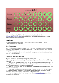


© Copyright 2026