ABC
docz
Explore
Log in
Create new account
Download
Report
science
biology
marine biology
ESCI 322 - Oceanography Laboratory Laboratory Manual
ESCI 322 - Oceanography Laboratory Laboratory Manual
Desalination: What is it and how does it work?
Why Study Optics? • Digital Cameras ~$24 Billion market
SSU Forecast: North Bay Recession to End This Summer
Finger Wave Hair Style Notes (Key) What is a Finger
SAMPLE PAPER 2011-12
decorating If you’re lucky enough to have a bay window, make the most
A bit of a deadbeat saves the day
Seawater sample collection:
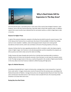
Why Is Real Estate Still So Expensive In The Bay Area?
ECSI, Inc. Employee Agreement This Agreement is entered into by
© Copyright 2026
About abcdocz
DMCA / GDPR
Report